Numerical Solutions of Space-Fractional Advection–Diffusion–Reaction Equations

Abstract

Background: solute transport in highly heterogeneous media and even neutron diffusion in nuclear environments are among the numerous applications of fractional differential equations (FDEs), being demonstrated by field experiments that solute concentration profiles exhibit anomalous non-Fickian growth rates and so-called “heavy tails”. Methods: a nonlinear-coupled 3D fractional hydro-mechanical model accounting for anomalous diffusion (FD) and advection–dispersion (FAD) for solute flux is described, accounting for a Riesz derivative treated through the Grünwald–Letnikow definition. Results: a long-tailed solute contaminant distribution is displayed due to the variation of flow velocity in both time and distance. Conclusions: a finite difference approximation is proposed to solve the problem in 1D domains, and subsequently, two scenarios are considered for numerical computations.

1. Introduction

Fractional and tempered fractional [1] differential equations (FDEs) have proved to be strong tools in the modelling of many physical phenomena, including acoustics and thermal systems and rheology and modelling of materials, leading to significant developments of analytical and numerical methods for solving fractional ordinary and partial differential equations in recent times. They comprise, e.g., Laplace–Fourier transform techniques and Green function approach [2], Lie symmetries theory and group analysis [3,4,5,6], Adomian decomposition [7,8], and homotopy perturbation methods [9], as well as finite element [10,11] and finite volume schemes [12,13], finite difference methods [14], and spectral ones [15,16,17,18].

Among the numerous applications in the various fields of science and engineering, we recall solute transport in highly heterogeneous media and even neutron diffusion in nuclear environments [19]. In fact, field experiments demonstrate that solute concentration profiles exhibit anomalous non-Fickian growth rates and so-called “heavy tails”, i.e., effects which cannot be predicted via the standard mass transport equation [20,21,22,23] but via fractional-order differential equations that may be viewed as long-time and long-space limits of a continuous time random walk (CTRW) [24]. Correspondingly, the Fickian advection–dispersion equation (ADE), unable to reflect the long tail dispersion process, is converted into a fractional one (FADE). The FADE approach appears to have the potential to predict non-Fickian dispersion processes, but its wide application is delayed by the difficulty to both obtain analytical solutions, especially when reaction terms are incorporated [25,26] or kernel non-singularities occur [27], and increased computational costs. Again, when considering water flow in low-permeability porous media, a nonlinear relationship between water flux and hydraulic gradient should be considered, thereby indicating a non-Darcian flow. Hence, for developing a more appropriate description able to include a memory effect, the existing relationships can be modified in a fractional fashion [24,28].

In case of time-fractional neutron diffusion models with delayed neutrons [19,29,30], non-local effects are established and sub-diffusive phenomena caught, coming from the heterogeneity of nuclear reactors. Anyway, analytical solutions for this problem are generally not available and only a few efficient numerical techniques have been developed in the literature to approximate the solution of even a 2D fractional [10,31] or non-fractional [32] diffusion models, even in the presence of a reaction term [26,33]. Alternatively, non-local problems accounting for long-range interactions can be treated via non-local integral models [34] and even combined time-fractional and space-nonlocal strategies [35].

Starting from an already-available 3D hydro-mechanical model in finite strains based on the modified mixture theory [36], an upgraded fractional version is proposed here, accounting for a fractional constitutive equation for both pore fluid and solute transport. Correspondingly, the model is suitable for performing anomalous diffusion (FD) and advection–dispersion–reaction (FADR) analyses; however, more importantly, the present formulation innovatively includes the contribution of deformation non-linearities for the solid skeleton, as well as a strain-dependent permeability tensor. Additionally, a modified finite difference algorithm is proposed to solve the problem in 1D domains, adopting the fractional-centered derivative scheme combined with the β-method, with the advective term treated via a Lax–Wendroff scheme. When accounting for advection–dispersion phenomena, including overpressure effects, the numerical algorithm was enriched by the split operator method [24,25]. Hence, the advection step was solved via an explicit second-order midpoint method, together with the β-method for the fractional diffusion–dispersion step and the trapezoidal rule for the fluid excess step. The algorithm additionally shifts into a backward implicit one in case of long-term analyses. Literature results are used to validate the model, and are subsequently applied for simulating radionuclide transport processes within cemented materials.

2. Materials and Methods

Fractional Constitutive Equations for Pore Fluid and Solute Transport

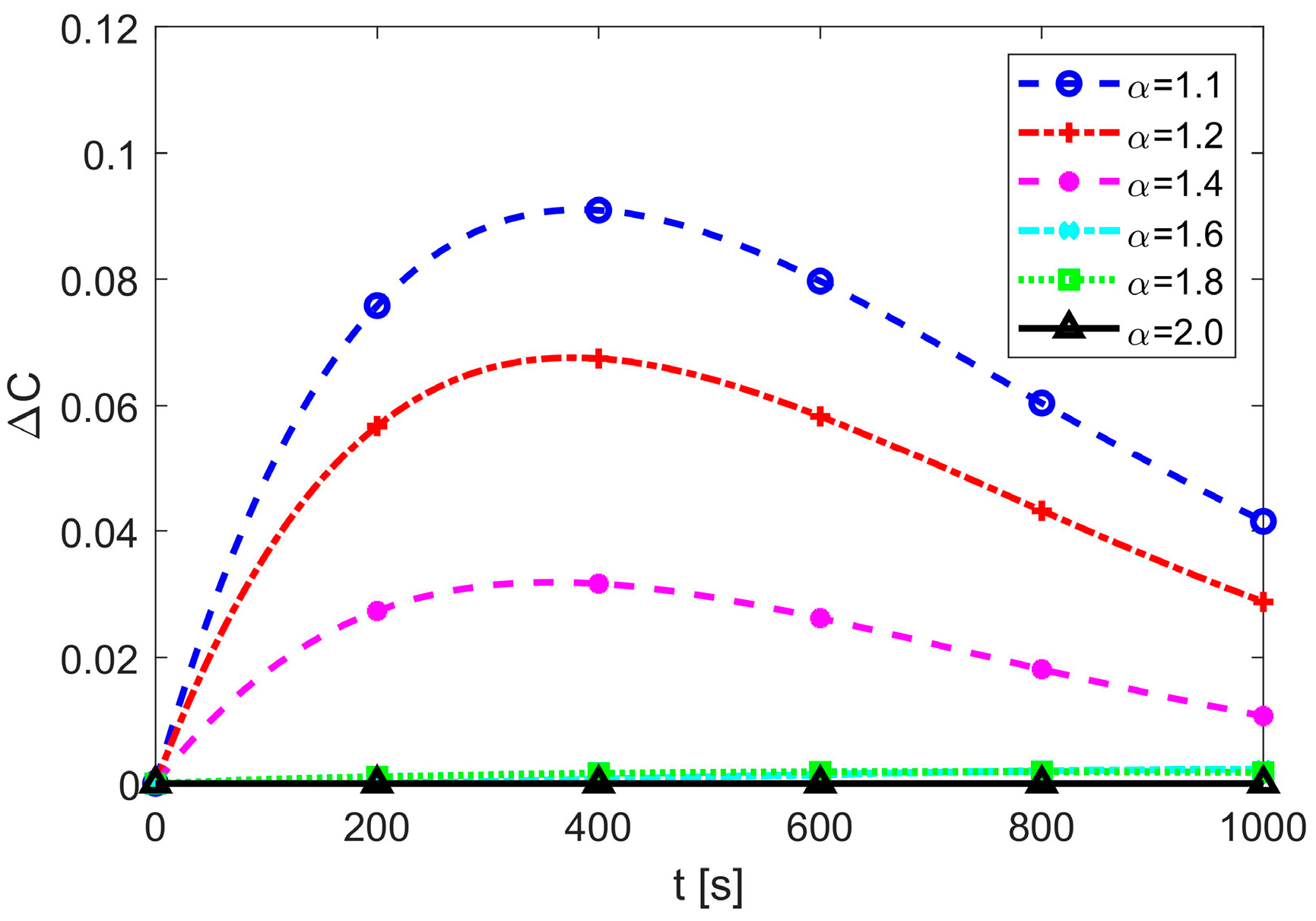
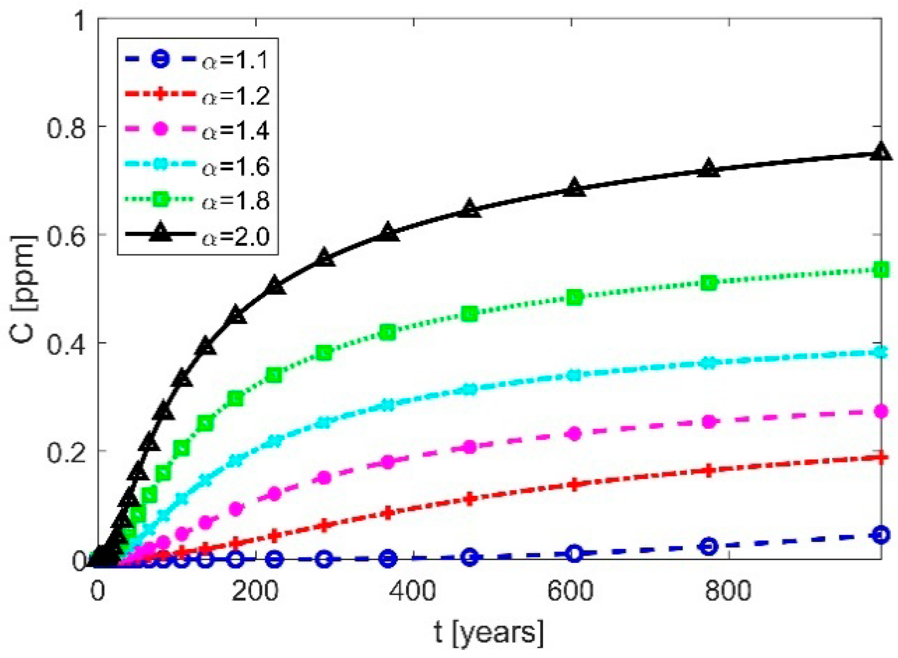
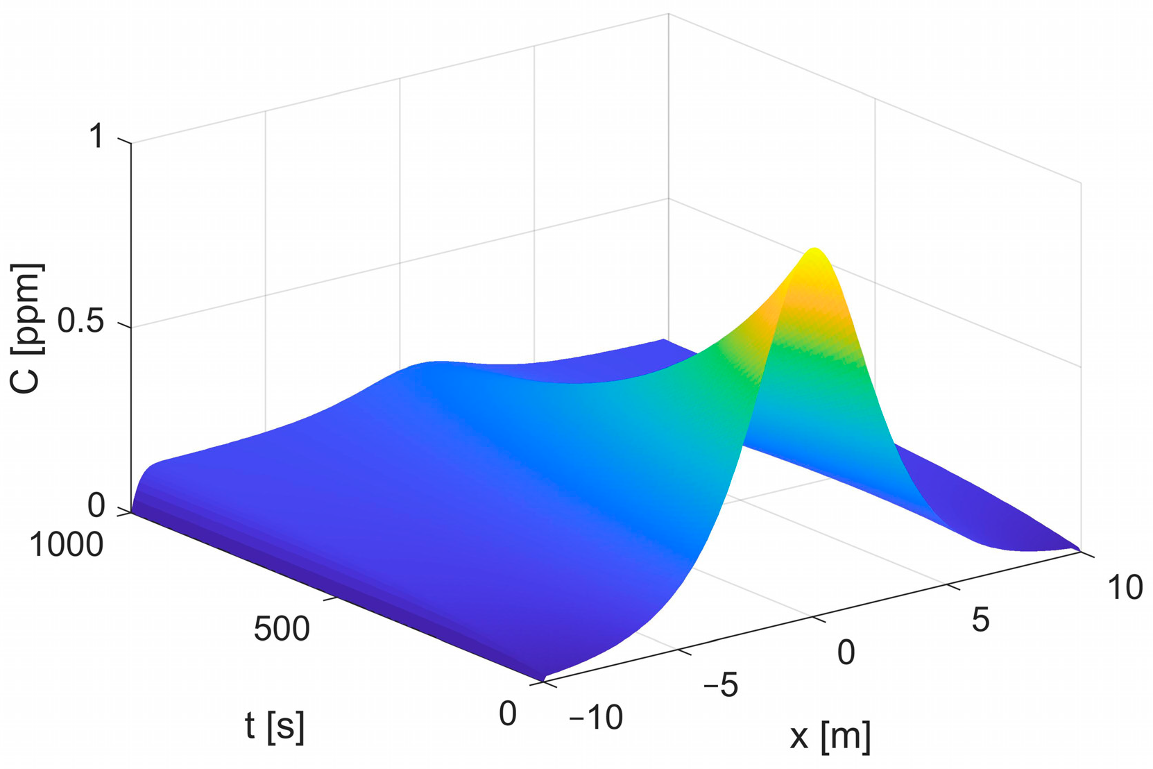
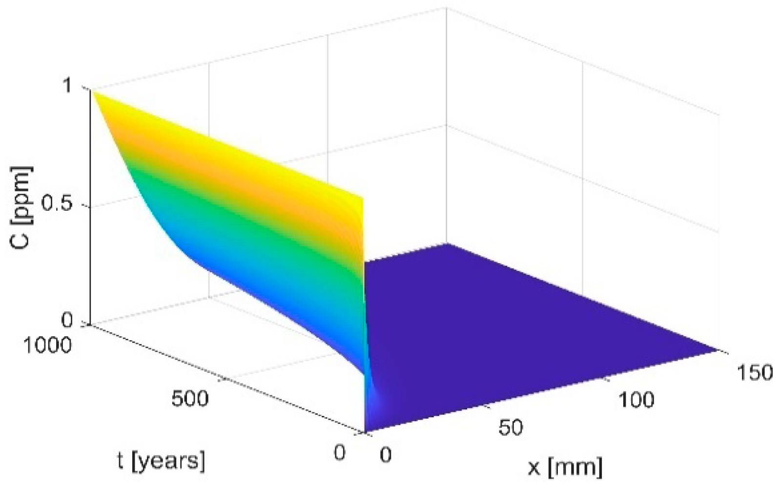
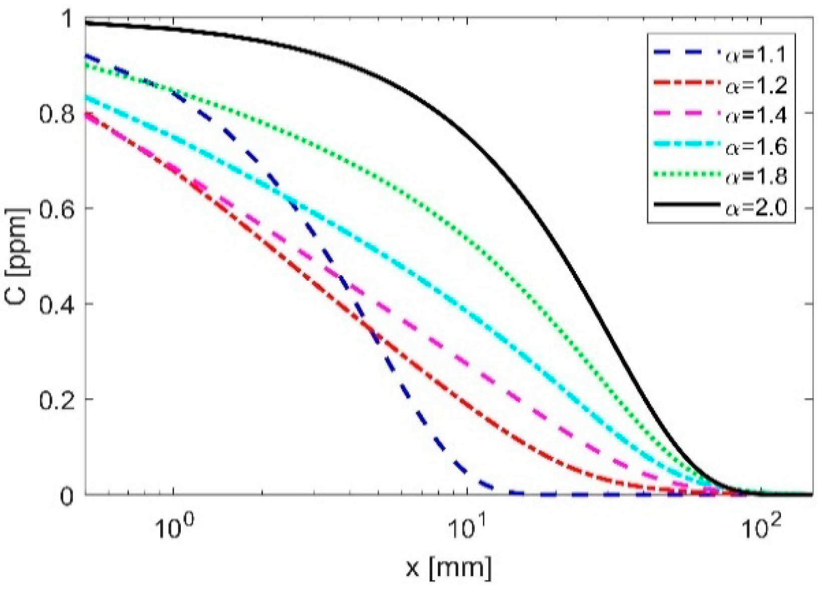
Darcy’s law is used to describe the flow of fluids in porous media within the local fluid content continuity equation in isothermal and fully saturated conditions, i.e., [36].

$$\nabla \cdot v-\frac{1}{{\rho }_w}\nabla \cdot \left({\rho }_w\frac{k}{\mu }\cdot \left(\nabla p-{\rho }_{w}g\right)\right)=0.$$

(1)

The porous medium is treated as inhomogeneous thanks to the adoption of fractional-order density gradients so to recover, at least at the phenomenological level, nonlocal (long-range) diffusion effects [37,38,39]. Time/space-fractional derivatives are proposed to describe anomalous dispersion, induced by fluid motion stacked around porous media inhomogeneities, e.g., fractures. This phenomenon is reflected as non-Gaussian particle dispersion with heavy tails [40].

Correspondingly, Equation (1) becomes

$${\rho }_w\nabla \cdot v-\nabla \cdot \left({\rho }_w\frac{k}{\mu }\cdot \left({\nabla }^{\alpha -1}p-{\rho }_{w}g\right)\right)=0,$$

(2)

choosing the Grünwald definition for fractional derivative [25] which appears convenient for numerical solutions [41], so that the value of a fractional differential operator acting on the generic function Ψ(x, t) is an infinite series, i.e.,

$$\frac{{\partial }^{\alpha }\mathsf{\Psi }(x,t)}{\partial x^{\alpha }}=\underset{N\to \infty }{\lim }\frac{1}{h^{\alpha }\Gamma (-\alpha )}{\displaystyle \sum _{j=0}^{N-1}\frac{\Gamma (j-\alpha )}{\Gamma (j+1)}\mathsf{\Psi }(x+\frac{\alpha }{2}h-jh,t)},$$

(3)

in which h = Δx = x/N, N is a positive integer.

It is to be noted that the fractor, α, physically reflects the heterogeneity of the soil medium in which solute is transported, and, for isotropic media, α = 2, i.e., the more heterogeneous the medium, the smaller than the integer constant of 2. Its decrease reproduces an increase in the resistance of the medium to solute dispersion and transport, leading to a delay in the phenomenon.

The combined solute transport within the non-linear deformable matrix-fluid system can be written as [24]

$$(1-\varphi )J\dot{C}\left({\rho }_s{K}_d-1\right)+JC\nabla \cdot v=-\nabla \cdot \left[\varphi {\rho }_{w}C\left(\frac{k}{\mu }\cdot \left({\nabla }^{\alpha -1}p-{\rho }_{w}g\right)\right)\right]+\frac{\varphi D}{J}\cdot {\nabla }^{\alpha }C,$$

(4)

by having extended the approaches [42,43] to 3D domains and J = det(F) > 0, with F(X, t) being the deformation gradient of the solid skeleton.

Equation (4) neglects the effect of sorption (being the medium in saturated conditions), so that the concentration of solute in the solid phase can be assumed to be linearly dependent on the concentration of the solute in the pore fluid via the contaminant partitioning coefficient.

The system of FADE (2) (4) becomes partly uncoupled due to the independence of the transport equation for pore fluid on the solute concentration, so that the pressure values can be treated as known data within Equation (4). Additionally, having already studied the contribution of anomalous water diffusion elsewhere [24], it is assumed to associate the fractional feature to the contaminant only. Hence, by introducing Equation (2) into Equation (4) and neglecting spatial non-linearities for fluid properties, the 1D non-linear saturated model is governed by

$$(1-\varphi )J\left({\rho }_s{K}_d-1\right)\dot{C}+\left(\varphi {\rho }_w\frac{k}{\mu }\frac{\partial p}{\partial x}\right)\frac{\partial C}{\partial x}+\left(J+\varphi {\rho }_w\right)\frac{k}{\mu }\frac{{\partial }^{2}p}{\partial x^2}C-\frac{\varphi D}{J}\cdot {\nabla }^{\alpha }C=0.$$

(5)

Similar observations can be carried out for the jacobian, which introduces an additional coupling with the mechanical part; in fact, recalling that $\vartheta =\ln J$, the jacobian results directly related to pore pressure through [24]

$$\vartheta \approx \frac{p-p_0-{\sigma }_0}{\kappa +\frac{4}{3}G},$$

(6)

so even itself can be treated as a known term (Expression (6) is valid under the assumptions of negligible self-weight and isothermal conditions).

Equation (5) involves effectively three processes of solute transport: the second term denotes advection caused by fluid flow; the third term reflects the transfer of solute resulting from pore fluid excess; and the fractional-order derivative term represents the contribution of dispersion in a heterogeneous medium. After rearrangement, we obtain

$$\frac{\partial \overline{C}}{\partial t}+\overline{u}\frac{\partial \overline{C}}{\partial x}+\overline{Y}\overline{C}-\overline{K}\cdot {\nabla }^{\alpha }\overline{C}=0,$$

(7)

with

$$\overline{u}=\frac{\varphi {\rho }_{w}k}{(1-\varphi )J\left({\rho }_s{K}_d-1\right)\mu }\frac{\partial p}{\partial x},\hspace{1em}\overline{Y}=\frac{{\overline{Q}}_f+\left(J+\varphi {\rho }_w\right)\frac{k}{\mu }\frac{{\partial }^{2}p}{\partial x^2}}{(1-\varphi )J\left({\rho }_s{K}_d-1\right)},\hspace{1em}\overline{K}=\frac{\varphi D}{J^2(1-\varphi )\left({\rho }_s{K}_d-1\right)}.$$

(8)

It is to be noticed that Equation (7) has general validity and, considering expression (8), shows variable coefficients, leading to a nonlinear structure; for simplicity, in the following we assume linear-type pore pressure distributions, permeability weakly dependent on deformation, together with small volume changes. Such an assumption has helped to validate the model against available results, as reported below.

Solving the FADE (7) for the transport rate $\overline{C}$ [44,45], including solute transport by pore fluid excess $\overline{Y}\overline{C}$, requires the adoption of a proper numerical strategy; as stated previously, it is here assumed to refer to the Grünwald definition of the fractional derivative, Equation (3), particularly referring to the shifted Grünwald–Letnikow formula [41]. Correspondingly, the final iterative system now becomes

$$(I+\beta A-\beta B)C^{t+1}=[I-(1-\beta )A+(1-\beta )B]C^t+(F^t+\beta \Delta F)\Delta t,$$

(9)

with

$$\begin{array}{l}B=\frac{\overline{K}}{2}\frac{\Delta t}{\Delta x^{\alpha }}\left[(1+\gamma )L+(1-\gamma )L^T\right]\hspace{1em}\hspace{1em}\hspace{1em}\hspace{1em}L=\left[\begin{array}{ccccc}{p}_1& p_0& 0& \cdots & 0\\ p_2& p_1& p_0& \cdots & 0\\ p_3& p_2& p_1& \cdots & 0\\ ⋮& ⋮& ⋮& \ddots & ⋮\\ p_N& p_{N-1}& p_{N-2}& \cdots & p_0\\ 0& p_N& p_{N-1}& \cdots & p_1\end{array}\right]\\ p_N=-\frac{\Gamma (N-\alpha )}{\Gamma (-\alpha )\Gamma (N+1)}\end{array}$$

(10)

where γ is a parameter accounting for the distribution probability of the relative weight of solute particle, and A is a tridiagonal matrix related to the discretization of the advective term via the Lax–Wendroff scheme [46].

$$A=\left[\begin{array}{ccccc}{v}^2& -\frac{v(v-1)}{2}& 0& \dots & 0\\ -\frac{v(v+1)}{2}& v^2& -\frac{v(v-1)}{2}& \dots & 0\\ 0& -\frac{v(v+1)}{2}& v^2& \dots & 0\\ ⋮& ⋮& ⋮& \ddots & -\frac{v(v-1)}{2}\\ 0& 0& 0& -\frac{v(v+1)}{2}& v^2\end{array}\right],\hspace{1em}\hspace{1em}\hspace{1em}v=V\frac{\Delta t}{\Delta x},$$

(11)

where V is the average fluid velocity along x direction, substantially equivalent to the first term in Equation (8).

When accounting for pore fluid excess, the scheme proposed by [47] was followed, based on the split-operator method. In particular, it was assumed to solve the advection step via an explicit second-order midpoint method, the fractional diffusion/dispersion step via the aforementioned β-method, and the fluid excess step via the trapezoidal rule.

3. Results

Once validated, the fractional model against the numerical example of [48], taken as benchmark [24], suggests that a 1D situation of an advection–dispersion–reaction was first considered [47], driven by Equation (7), with the additional term $E({\overline{C}}_s-\overline{C})$ reflecting the transfer of solute from an active source (generally included when modelling overland solute transport)

$$\frac{\partial \overline{C}}{\partial t}+\overline{u}\frac{\partial \overline{C}}{\partial x}+\overline{Y}\overline{C}-\overline{K}\cdot {\nabla }^{\alpha }\overline{C}-E({\overline{C}}_s-\overline{C})=0,$$

(12)

being

$$\begin{array}{l}{\overline{C}}_s=C_0{e}^{-\overline{\mu }t}\\ {\overline{C}}_s(x,0)=C_0(x)\end{array}$$

(13)

As assumed by the data reported in

Table 1. Material parameters for FADR analysis.

Parameter	Values	Unit [-]
a	−10	m
b	10	m
$\overline{K}$	10−4	m2/s
v	0.5	m/s
E	0.02	s−1
$\overline{\mu }$	0.0001	s−1
N	200	-
T	100	-
tend	1000	s

, together with an initial condition C₀ = 0.5, Figure 1 depicts the spatial–temporal distribution of concentration in the case of a standard ADR (non-fractional) solution, whereas Figure 2 evidences the fractional effect, producing a greater and slightly delayed peak with decreasing fractor alpha (maximum 10%). This seems to confirm (as experienced in [47]) that the ADR model generally predicts a faster flushing process of solute as compared to the FADR one, considering that the fractional approach allows to account for the material heterogeneity.

To additionally test the contribution of a fractional model, a log-term low-waste radionuclides transport process within cemented materials is considered. The transport rate through engineered barriers (compacted bentonite clay and cement) is mainly diffusion-controlled; however, due to the strong sorption behavior of the materials, the diffusion rate of the radionuclides is much slower than in pure water. Particularly, the case reported in [49] is reconstructed via a fractional approach, with material data of

Table 2. Material parameters for FD radionuclides transport.

Parameter	Values	Unit [-]
a	0	mm
b	150	mm
$\overline{K}$	10−4	m2/s
N	300	-
t0	10−5	y
tend	993	y

and C(x,0) = 0. The backward-time implicit scheme is used with variable time steps, such that t_n+1 = 1.0125·Δt_n.

The classical non-fractional solution is newly obtained in terms of the distribution of spatial–temporal radionuclides concentration (Figure 3). Interestingly, change in the transport mechanism can be noticed once fractors are lower than 1.6 and particularly when lower than 1.2 (Figure 4). A slower diffusion process is found again, suggesting that possibly thinner cement containers could be required for ensuring the same safety level and degraded zone as the standard AD model. The heterogeneous cement matrix may, in fact, form hierarchical storage-release zones of nuclides, leading to a delayed transport process of the contaminant (Figure 5).

4. Discussion

A nonlinear coupled 3D fractional hydro-mechanical model accounting for anomalous diffusion (FD) and advection–dispersion (FAD) for solute flux is presented, accounting for a Riesz derivative treated through the Grünwald–Letnikow definition. The formulation innovatively includes the contribution of deformation non-linearities for the solid skeleton, as well as a strain-dependent permeability tensor. A finite difference approximation is built on purpose for modeling 1D domains and adopting the fractional-centered derivative scheme combined with the β-method, with the advective term treated via the Lax–Wendroff scheme. In particular, the algorithm shifts into a backward-time implicit one with variable time steps in case of long-term contaminants (radionuclides) transport. Under the assumptions of linear-type pore pressure distributions, permeability which is weakly dependent on deformation, together with small volume changes, means that the effects of the fractional dispersion term are analyzed.

A delayed release of solute pollutants or a long-tailed dispersion process caused by volume heterogeneities of the porous media was successfully described, evidencing a general gradual and slower solute contaminant transport. Additionally, when accounting for radionuclides transport within cemented materials and decreasing fractors, the model evidences a sort of solute-clog, with higher solute gradients and increasing solute levels. Correspondingly, it appears to be particularly suitable for reconstructing phenomena in which the kinetics of diffusion are slower than the kinetics of reaction and layers of very low solubility form and do not dissolve on observable time scales.

References

1. Sultana, F.; Singh, D.; Pandey, R.K.; Zeidan, D. Numerical schemes for a class of tempered fractional integro-differential equations. Appl. Num. Math. 2020, 157, 110–134. [Google Scholar] [CrossRef]
2. Miller, K.S.; Ross, B. An Introduction to the Fractional Calculus and Fractional Differential Equations; Wiley-Interscience: New York, NY, USA, 1993. [Google Scholar]
3. Prakash, P.; Sahadevan, R. Lie symmetry analysis and exact solution of certain fractional ordinary differential equations. Nonlinear Dynam. 2017, 89, 305–319. [Google Scholar] [CrossRef]
4. Jannelli, A.; Ruggieri, M.; Speciale, M.P. Numerical solutions of space fractional advection–diffusion equation, with nonlinear source term. Appl. Numer. Math. 2020, 155, 93–102. [Google Scholar] [CrossRef]
5. Bira, B.; Mandal, H.; Zeidan, D. Exact solution of the time fractional variant Boussinesq-Burgers equations. Appl. Math. 2021, 66, 437–449. [Google Scholar] [CrossRef]
6. Mandal, H.; Bira, B.; Zeidan, D. Power Series Solution of Time-Fractional Majda-Biello System Using Lie Group Analysis. In Proceedings of the International Conference on Fractional Differtiation and its Applications (ICFDA), Amman, Jordan, 16–18 July 2018. [Google Scholar] [CrossRef]
7. Daftardar-Geji, V.; Jafari, H. Adomian decomposition: A tool for solving a system of fractional differential equations. J. Math. Anal. Appl. 2005, 301, 508–518. [Google Scholar] [CrossRef] [Green Version]
8. Zeidan, D.; Chau, C.K.; Lu, T.T. On the characteristic Adomian decomposition method for the Riemann problem. Math. Meth. Appl. Sci. 2021, 44, 8097–8112. [Google Scholar] [CrossRef]
9. Momani, S.; Odibat, Z. Homotopy perturbation method for nonlinear partial differential equations of fractional order. Phys. Lett. A 2007, 365, 345–350. [Google Scholar] [CrossRef]
10. Zhang, N.; Deng, W.; Wu, Y. Finite difference/element method for a two-dimensional modified fractional diffusion equation. Adv. Appl. Math. Mech. 2012, 4, 496–518. [Google Scholar] [CrossRef]
11. Liu, Y.; Yu, Z.D.; Li, H.; Liu, F.W.; Wang, J.F. Time two-mesh algorithm combined with finite element method for time fractional water wave model. Int. J. Heat Mass Transfer 2018, 120, 1132–1145. [Google Scholar] [CrossRef]
12. Hejazi, H.; Moroney, T.; Liu, F. Stability and convergence of a finite volume method for the space fractional advection–dispersion equation. J. Comput. Appl. Math. 2014, 684–697. [Google Scholar] [CrossRef] [Green Version]
13. Li, F.; Fu, H.; Liu, J. An efficient quadratic finite volume method for variable coefficient Riesz space-fractional diffusion equations. Math. Methods Appl. Sci. 2021, 44, 2934–2951. [Google Scholar] [CrossRef]
14. Zhou, Y.; Suzuki, J.L.; Zhang, C.; Zayernouri, M. Implicit-explicit time integration of nonlinear fractional differential equations. Appl. Numer. Math. 2020, 156, 555–583. [Google Scholar] [CrossRef]
15. Doha, E.H.; Bhrawy, A.H.; Baleanu, D.; Ezz-Eldien, S.S. Numerical schemes with high spatial accuracy for a variable-order anomalous subdiffusion equation. Appl. Math. Comput. 2013, 219, 8042–8056. [Google Scholar]
16. Zhao, T.; Mao, Z.; Karniadakis, G.E. Multi-domain spectral collocation method for variable-order nonlinear fractional differential equations. Comput. Methods Appl. Mech. Engrg. 2019, 348, 377–395. [Google Scholar] [CrossRef] [Green Version]
17. Zaky, M.A.; Hendy, A.S.; Macias-Diaz, J.E. Semi-implicit Galerkin–Legendre spectral schemes for nonlinear time-space fractional diffusion–reaction equations with smooth and nonsmooth solutions. J. Sci. Comput. 2020, 82, 13. [Google Scholar] [CrossRef]
18. Dwivedi, K.D.; Das, S.; Baleanu, D. Numerical solution of nonlinear space–time fractional-order advection–reaction–diffusion equation. J. Comput. Nonlinear Dynam. 2020, 15, 061005. [Google Scholar] [CrossRef]
19. Roul, P.; Rohil, V.; Espinosa-Paredes, G.; Obaidurrahman, K. Numerical simulation of two-dimensional fractional neutron diffusion model describing dynamical behaviour of sodium-cooled fast reactor. Ann. Nuclear Energy 2021, 166, 108709. [Google Scholar] [CrossRef]
20. Schumer, R.; Benson, D.A.; Meerschaert, M.M.; Baeumer, B. Fractal mobile/immobile transport. Water Res. Res. 2003, 39, 1296. [Google Scholar]
21. Zhang, Y.; Benson, D.A.; Reeves, D.M. Time and space non-localities underlying fractional-derivative models: Distinction and literature review of field applications. Adv. Wat. Res. 2009, 32, 561–581. [Google Scholar] [CrossRef]
22. Fomin, S.; Chugunov, V.; Hashida, T. The effect of non-Fickian diffusion for modelling the anomalous diffusion of contaminant from fracture into porous rock matrix with bordering alteration zone. Transp. Por. Media 2010, 81, 187–205. [Google Scholar] [CrossRef]
23. Fomin, S.A.; Chugunov, V.A.; Hashida, T. Non-Fickian mass transport in fractured porous media. Adv. Wat. Res. 2011, 34, 205–214. [Google Scholar] [CrossRef]
24. Salomoni, V.A.; De Marchi, N. A three-dimensional finite strain model of solute transport in saturated porous media with a fractional approach. J. Eng. Sci. 2021; under review. [Google Scholar]
25. Deng, Z.Q.; Singh, V.P.; Bengtsson, L. Numerical solution of fractional advection-dispersion equation. J. Hydr. Engrg. 2004, 130, 422–431. [Google Scholar] [CrossRef] [Green Version]
26. Kumar, S.; Zeidan, D. An efficient Mittag-Leffler kernel approach for time-fractional advection-reaction-diffusion equation. Appl. Num. Math. 2021, 170, 190–207. [Google Scholar] [CrossRef]
27. Yavuz, M.; Ozdemir, N. An Integral Transform Solution for Fractional Advection-Diffusion Problem. In Proceedings of the International Conference on Mathematical Studies and Applications, Karaman, Turkey, 4–6 October 2018; pp. 442–446. [Google Scholar]
28. Zhou, H.W.; Yang, S.; Zhang, S.Q. Modeling non-Darcian flow and solute transport in porous media with the Caputo-Fabrizio derivative. Appl. Math. Mod. 2009, 68, 603–615. [Google Scholar] [CrossRef]
29. Roul, P.; Rohil, V.; Espinosa-Paredes, G.; Prasad Goura, V.M.K.; Gedam, R.S.; Obaidurrahman, K. Design and analysis of a numerical method for fractional neutron diffusion equation with delayed neutrons. Appl. Numer. Math. 2020, 157, 634–653. [Google Scholar] [CrossRef]
30. Roul, P.; Rohil, V.; Espinosa-Paredes, G.; Obaidurrahman, K. An efficient numerical method for fractional neutron diffusion equation in the presence of different types of reactivities. Ann. Nucl. Energy 2021, 152, 108038. [Google Scholar] [CrossRef]
31. Kuila, S.; Raja Sekhar, T.; Zeidan, D. On the Riemann Problem Simulation for the Drift-Flux Equations of Two-Phase Flows. Int. J. Com. Meth. 2016, 13, 1650009. [Google Scholar] [CrossRef] [Green Version]
32. Zeidan, D.; Romenski, E.; Slaouti, A.; Toro, E.F. Numerical study of wave propagation in compressible two-phase flow. Int. J. Num. Meth. Fluids 2007, 54, 393–417. [Google Scholar] [CrossRef]
33. Erdogan, U.; Sari, M.; Kocak, H. Efficient numerical treatment of nonlinearities in the advection–diffusion–reaction equations. Int. J. Num. Meth. Heat Fluid Flow 2019, 29, 132–145. [Google Scholar] [CrossRef]
34. Pinnola, F.P.; Vaccaro, M.S.; Barretta, R.; Marotti de Sciarra, F. Random vibrations of stress-driven nonlocal beams with external damping. Meccanica 2021, 56, 1329–1344. [Google Scholar] [CrossRef]
35. Barretta, R.; Marotti de Sciarra, F.; Pinnola, F.P.; Vaccaro, M.S. On the nonlocal bending problem with fractional hereditariness. Meccanica 2021. [Google Scholar] [CrossRef]
36. Salomoni, V.A. A mathematical framework for modelling 3D coupled THM phenomena within saturated porous media undergoing finite strains. Comp. Part B Eng. 2018, 146, 42–48. [Google Scholar] [CrossRef]
37. He, J.H. Approximate analytical solution for seepage flow with fractional derivatives in porous media. Comput. Meth. Appl. Mech. Eng. 1998, 167, 57–68. [Google Scholar] [CrossRef]
38. Schumer, R.; Benson, D.A.; Meerschaert, M.M.; Wheatcraft, S.W. Eulerian derivation of the fractional advection–dispersion equation. J. Contam. Hydrol. 2001, 48, 69–88. [Google Scholar] [CrossRef]
39. Ochoa-Tapia, J.A.; Valdes-Parada, F.J.; Alvarez-Ramirez, J. A fractional-order Darcy’s law. Phys. A Stat. Mech. Appl. 2007, 374, 1–14. [Google Scholar] [CrossRef]
40. Cushman, J.H.; Moroni, M. Statistical mechanics with three-dimensional particle tracking velocimetry experiments in the study of anomalous dispersion I: Theory. Phys. Fluids 2001, 13, 75–80. [Google Scholar] [CrossRef]
41. Oldham, K.B.; Spanier, J. The Fractional Calculus; Academic Press: New York, NY, USA, 1974. [Google Scholar]
42. Zhang, H.J.; Jeng, D.S.; Barry, D.A.; Seymour, B.R.; Li, L. Solute transport in nearly saturated porous media under landfill clay liners: A finite deformation approach. J. Hydrol. 2013, 479, 189–199. [Google Scholar] [CrossRef]
43. Peters, G.P.; Smith, D.W. Solute transport through a deforming porous medium. Int. J. Num. An. Meth. Geomech. 2002, 26, 683–717. [Google Scholar] [CrossRef]
44. Chaves, A.S. A fractional diffusion equation to describe Levy flights. Phys. Lett. A 1998, 239, 13–16. [Google Scholar] [CrossRef]
45. Benson, D.A.; Wheatcraft, S.W.; Meerschaert, M.M. The fractional-order governing equation of Levy motion. Water Resour. Res. 2000, 36, 1413–1423. [Google Scholar] [CrossRef]
46. Owolabi, K.M.; Atangana, A. Numerical Methods for Fractional Differentiation; Springer: Singapore, 2019. [Google Scholar]
47. Deng, Z.Q.; de Lima, J.L.M.P.; de Lima, M.I.P.; Singh, V.P. A fractional dispersion model for overland solute transport. Water Resour. Res. 2006, 42, W03416. [Google Scholar] [CrossRef] [Green Version]
48. Çelik, C.; Duman, M. Crank–Nicolson method for the fractional diffusion equation with the Riesz fractional derivative. J. Comp. Phys. 2012, 231, 1743–1750. [Google Scholar] [CrossRef]
49. Salomoni, V.A.; Majorana, C.E. Parametric analysis of diffusion of activated sources in disposal forms. J. Haz. Mat. 2004, A113, 45–56. [Google Scholar]
Figure 1. Concentration distribution (standard ADR model).
Fractalfract 06 00021 g001
Figure 2. Time history of relative concentration variation at a reference point.
Fractalfract 06 00021 g002
Figure 3. Radionuclide distribution (standard AD model).
Fractalfract 06 00021 g003
Figure 4. Spatial distribution of low-level radionuclides at a reference time-step.
Fractalfract 06 00021 g004
Figure 5. Time history of radionuclides at a reference node.
Fractalfract 06 00021 g005