Article

Scaling in Anti-Plane Elasticity on Random Shear Modulus Fields with Fractal and Hurst Effects

by
Yaswanth Sai Jetti
1 and
Martin Ostoja-Starzewski
1,2,3,*
1
Department of Mechanical Science & Engineering, University of Illinois at Urbana-Champaign, Urbana, IL 61801, USA
2
Institute for Condensed Matter Theory, University of Illinois at Urbana-Champaign, Urbana, IL 61801, USA
3
Beckman Institute for Advanced Science and Technology, University of Illinois at Urbana-Champaign, Urbana, IL 61801, USA
*
Author to whom correspondence should be addressed.
Fractal Fract. 2021, 5(4), 255; https://doi.org/10.3390/fractalfract5040255
Submission received: 28 October 2021 / Revised: 28 November 2021 / Accepted: 30 November 2021 / Published: 4 December 2021
(This article belongs to the Special Issue 2021 Feature Papers by Fractal Fract's Editorial Board Members)

Abstract

:
The scale dependence of the effective anti-plane shear modulus response in microstructures with statistical ergodicity and spatial wide-sense stationarity is investigated. In particular, Cauchy and Dagum autocorrelation functions which can decouple the fractal and the Hurst effects are used to describe the random shear modulus fields. The resulting stochastic boundary value problems (BVPs) are set up in line with the Hill–Mandel condition of elastostatics for different sizes of statistical volume elements (SVEs). These BVPs are solved using a physics-based cellular automaton (CA) method that is applicable for anti-plane elasticity to study the scaling of SVEs towards a representative volume element (RVE). This progression from SVE to RVE is described through a scaling function, which is best approximated by the same form as the Cauchy and Dagum autocorrelation functions. The scaling function is obtained by fitting the scaling data from simulations conducted over a large number of random field realizations. The numerical simulation results show that the scaling function is strongly dependent on the fractal dimension D, the Hurst parameter H, and the mesoscale δ , and is weakly dependent on the autocorrelation function. Specifically, it is found that a larger D and a smaller H results in a higher rate of convergence towards an RVE with respect to δ .

1. Introduction

The continuum mechanical properties of any natural or engineering material are dependent on the material’s physical structure at various scales below the macroscopic (or continuum). Thus, any continuum model corresponds to having effective (or averaged) properties of the heterogeneous substructure in some manner. The pertinent number of length scales and the relevant characteristics of substructure at each scale for obtaining these effective properties vary greatly from one material to another. One of the major challenges lies in homogenization, whose goal is to develop the phenomenological constitutive equations for the macroscopic response of idealized continua with heterogeneous substructures. The problem of homogenization for heterogeneous materials with linear mechanical and thermal properties has been studied extensively, with the conventional focus being on the effective (or macroscopic) responses of two or multi-phase random composites. This is the case for a representative volume element (RVE), as opposed to the statistical volume element (SVE), for which one is additionally interested in establishing the scaling to RVE [1,2]. Key papers in research on the SVE are [3,4].
In recent years, extensive literature has been produced on the computation of effective properties based on Monte-Carlo type simulations in various fields [5,6,7,8,9,10,11,12,13,14]. In the context of elasticity, Murshed et al. [7] obtained rigorous bounds on randomly distributed elastic polycrystals comprised of lower symmetry single crystals. Kale et al. [9] studied the scale-dependent bounds on the effective thermal conductivity of 2d Gaussian correlated microstructures. Savvas et al. [12] coupled an extended finite element method with Monte-Carlo simulations to determine effective stiffness and compliance elasticity tensors in random composites with differences in local volume fraction. Recently, Karimi et al. [14] investigated electrostatic and magnetostatic properties of 2d and 3d two-phase media after adapting Hill–Mandel conditions to electric and magnetic fields.
The present investigation focuses on the effects of fractal and Hurst characteristics of random media [15] on the scaling of their elastic properties when going from SVE to RVE. This is beyond all the previous studies that assumed either white-noise or very short-range correlations. Our study is focused on the anti-plane elasticity of media modeled by random fields of local shear modulus. Let the SVE in 2d be characterized by a mesoscale: a ratio of L = volume of SVE relative to the smallest heterogeneity size d. We ask: how do the random fluctuations in response to the SVE diminish to zero with mesoscale L increasing? This diminishing signifies attaining the effective deterministic response. This leads to stochastic partial differential equations under either Dirichlet or Neumann boundary conditions. The random fields are specified through Cauchy and Dagum autocorrelation functions which allow independent choices of fractal and Hurst characteristics. We employ a physics-based cellular automaton, a numerical method in which it is convenient to introduce randomness on a discretized domain, to solve the stochastic BVPs. From this, we obtain scale-dependent bounds on the effective shear modulus response at multiple length scales for various combinations of fractal and Hurst parameters.
This article is organized as follows. In Section 2, we first establish the governing equations, and discuss the Hill–Mandel conditions for elastostatics. We then introduce the concepts of apparent and effective properties and that of the scaling function. Next, we discuss the Cauchy and Dagum random fields that define the microstructure in this study, followed by an overview of the cellular automaton method that is applicable to anti-plane elasticity. Section 3 presents and discusses the homogenization results over a wide range of fractal and Hurst parameters for various SVE sizes. The major findings and conclusions are outlined in Section 4.

2. Theory

2.1. Governing Equations

Consider a random mesoscale body, B δ = { B δ ( ω ) ; ω Ω } , where B δ ( ω ) is a specific realization corresponding to the sample event ω in the Ω space. The dimensionless parameter δ = L / d characterizes the mesoscale, where L is the domain (window) size. Focusing on the quasi-static loading with negligible body forces, we have the following governing equation of local equilibrium:
· σ = 0 ,
where σ is the the Cauchy stress field in the body, B δ ( ω ) . Let the strain field in B δ ( ω ) be ϵ . The present study focuses on anti-plane linear elasticity for B δ R 2 , so the equilibrium equation becomes:
· ( C ( x , ω ) u ) = 0 , x B δ ( ω ) .
In general, C ( x , ω ) is the stiffness tensor random field (TRF) [16] and u u 3 ( x , y ) is the anti-plane displacement. Equation (2) reduces to a stochastic generalization of the Navier–Cauchy equation of elastostatics. We consider the TRF C ( x , ω ) = c ( x , ω ) I to be locally isotropic, where I is a second-rank identity tensor and c ( x , ω ) is henceforth referred to as the random shear modulus. Thus, the TRF model is modeled directly by a scalar random field. The central issue addressed here concerns the scale-dependence of C as it is smoothed on ever larger scales, while assuming the fractal and Hurst properties for the finest scale resolution.

2.2. Scale-Dependent Homogenization

2.2.1. Hill–Mandel Macrohomogeneity Condition

The transition from micro to mesoscale is studied in terms of the so-called Hill–Mandel macrohomogeneity condition [17,18]. This condition requires the equivalence of the energetic and mechanical interpretations of spatially-averaged work performed on a material domain. If these interpretations give the same result for different uniform boundary conditions imposed on the domain, then we have an RVE, and if the material domain is too small, we have an SVE. To study this mesoscale ( L / d ) dependence, consider σ ¯ and ϵ ¯ to be the volume averages of σ and ϵ over the SVE. The Hill–Mandel macrohomogeneity condition reads [1]:
σ : ϵ ¯ = σ ¯ : ϵ ¯ B δ ( ω ) ( t σ ¯ · n ) ( u ϵ ¯ · x ) d S = 0 , x B δ ( ω ) .
where t and n are traction and normal vectors, respectively. The notation a : b = tr ( a T b ) denotes the tensor scalar product between two second order tensors a and b . Equation (3) is satisfied by three types of uniform boundary conditions [2,7,19]:
  • Uniform displacement (Dirichlet):
    u ( x ) = ϵ 0 · x , x B δ ( ω ) .
  • Uniform traction (Neumann):
    t ( x ) = σ 0 · n , x B δ ( ω ) .
  • Uniform displacement-traction (mixed-orthogonal):
    [ u ( x ) ϵ 0 · x ] · [ t ( x ) σ 0 · n ] = 0 , x B δ ( ω ) .
where ϵ 0 and σ 0 are constant strain and stress tensors, respectively. Note that ϵ 0 = ϵ ¯ and σ 0 = σ ¯ on account of the average strain and stress theorems [2].

2.2.2. Apparent and Effective Properties

At any particular mesoscale δ , upon solving the stochastic boundary value problem under the boundary conditions (4) or (5), and consequent ensemble averaging, results in a different apparent stiffness (or compliance) tensor. In the current work, the uniform displacement and the uniform traction boundary conditions are considered. Equation (4) results in the apparent stiffness tensor C δ d ( ω ) , where d stands for displacement boundary conditions. On the other hand, Equation (5) results in the apparent compliance tensor S δ t ( ω ) , where t stands for traction boundary conditions and note that C δ t ( ω ) S δ t ( ω ) 1 .
σ ¯ = C δ d ( ω ) : ϵ 0 ,
ϵ ¯ = S δ t ( ω ) : σ 0 .
As δ , the randomness vanishes and the tensor represent the macroscale effective elastic response C eff of an RVE. In general, C δ d ( ω ) , which gives an upper estimate for the effective stiffness, is different from C δ t ( ω ) , which gives a lower estimate for the effective stiffness [10]. Indeed, upon using the principles of minimum potential energy and complementary energy with the assumptions of spatial homogeneity and ergodicity of the random microstructure, one can obtain the heirarchy of δ -dependent bounds on C eff as follows [3,4]:
S 1 t 1 S δ t 1 S δ t 1 C eff C δ d C δ d C 1 d , δ < δ .
Upon using the definition of isotropic stiffness tensor along with Equation (9), we get the δ -dependent bounds on the shear modulus c eff as follows:
c R s 1 t 1 s δ t 1 s δ t 1 c eff c δ d c δ d c 1 d c V , δ < δ ,
where c R and c V are the Reuss (harmonic mean estimate of the shear modulus) and Voigt (arithmetic mean estimate of the shear modulus) estimates of the shear modulus.

2.2.3. Scaling

Consider the contraction between the apparent stiffness tensor and the apparent compliance tensor with the assumption of local isotropy for anti-plane elasticity in 2d:
C δ d : S δ t = 2 c δ d c δ t ,
lim δ C δ d : S δ t = 2 .
Following the previous studies, we postulate the following relation between the left-hand side of Equation (11) and the left-hand side of Equation (12):
C δ d : S δ t = lim δ C δ d : S δ t + g ( δ ) ,
g ( δ ) = 2 c δ d c δ t 1 ,
where g ( δ ) is the scaling function. Besides δ , it is also a function of the random microstructure. In general, g ( δ ) has two exact properties: (i) in the RVE limit: lim δ g δ = 0 ; (ii) for a homogeneous microstructure: g δ = 0 . The next step is to introduce the random fields that specify the random medium.

2.3. Random Fields

Many natural material properties are usually described through fractal behavior and Hurst effects. We introduce the randomness into the shear modulus fields, c ( x , ω ) , through two stochastic models, which can both capture and decouple fractal behavior and Hurst effects: Cauchy and Dagum [20,21,22,23]. The fractal dimension, D [ n , n + 1 ) , is a measure of roughness for a surface defined over R n . The larger is D, the rougher is the surface. The Hurst exponent or the Hurst parameter represents the “spatial memory.” In the case of a 1d RF (i.e., parametrization by R ), H [ 0 , 0.5 ) represents an anti-persistent system, H ( 0.5 , 1 ) represents a persistent system, and H = 0.5 corresponds to a true random walk. Both the Cauchy and Dagum shear modulus random fields are taken as Gaussian RFs, truncated to ensure the positive-definiteness of energy density.
The autocorrelation function for two random variables Z ( x 1 ) and Z ( x 2 ) , R : R 2 × R 2 R is:
R ( x 1 , x 2 ) = Z ( x 1 ) Z ( x 2 ) .
We consider random fields, which are wide-sense-stationary (WSS) and isotropic. Define r = x 1 x 2 , for the Cauchy class Gaussian random field, c ( x , ω ) , x R 2 , the generalized Cauchy correlation function [20] is
R α , β C ( x 1 , x 2 ) = R α , β ( r ) = ( 1 + r α ) β α , r 0 , α ( 0 , 2 ] , β > 0 .
The special case with α = 2 corresponds to the well-known Cauchy model [22]. The generalized Cauchy random field will be hereafter referred to as Cauchy random field following the nomenclature in [23]. The correlation function corresponding to Dagum random field is given as follows [23]:
R α , β D ( x 1 , x 2 ) = R α , β ( r ) = 1 ( 1 + r β ) α β , r 0 , α β , β ( 0 , 2 ] .
The fractal dimension (D) and the Hurst parameter (H) are related to ( n , α , β ) when α ( 0 , 2 ] and β ( 0 , 2 ) as follows:
D = n + 1 α 2 , H = 1 β 2 ,
where n = 2 for a 2d system. The special case when α = 2 β corresponds to a self-affine fractal. The power spectral density of the Cauchy random field is given in [24], and that of the Dagum random field is given in [25]. In the current study, the Cauchy and Dagum random fields are generated for various combinations of α and β . We used the so-called circulant embedding method [26] to generate the random fields in R software.

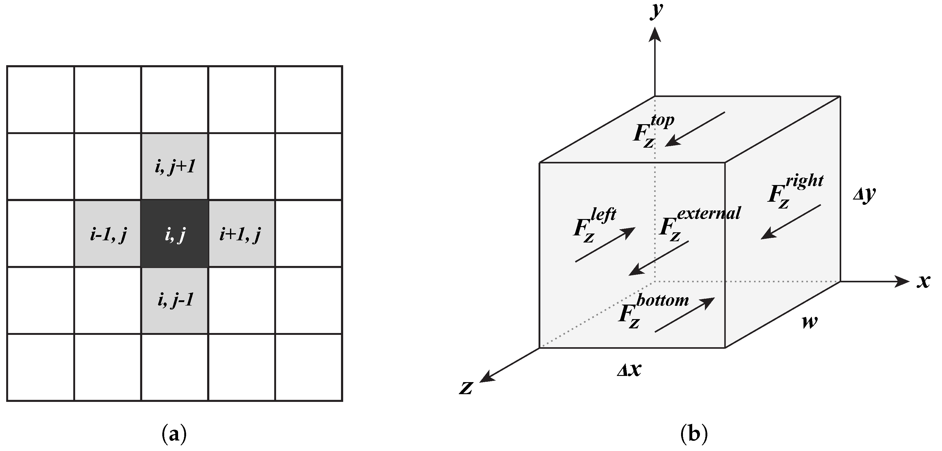
2.4. Cellular Automata

The cellular automaton (CA) method is a computational approach first proposed by John von Neumann [27]. Leamy [28] studied inplane elastodynamics using a physics-based rectangular-celled CA in an idealized linear elastic medium. Later Hopman et al. [29] extended this method to study arbitrary-shaped two-dimensional geometries. The application of CA to the anti-plane shear elastodynamic problem is studied by Xian et al. [30]. The rectangular-celled CA yields discrete equations which are mathematically equivalent to that of the centered-difference finite difference method. In CA, the computational domain is discretized into cells and the material properties are assigned to each cell making it convenient to introduce randomness to the shear modulus field.
Following [28,30], the CA formulation for anti-plane shear forces at cell ( i , j ) is given below:
F z t o p = ( w Δ x ) σ y z t o p = ( w Δ x ) c u z i , j + 1 u z i , j Δ y
F z b o t t o m = ( w Δ x ) σ y z b o t t o m = ( w Δ x ) c u z i , j u z i , j 1 Δ y
F z r i g h t = ( w Δ y ) σ x z r i g h t = ( w Δ y ) c u z i + 1 , j u z i , j Δ x
F z l e f t = ( w Δ y ) σ x z l e f t = ( w Δ y ) c u z i , j u z i 1 , j Δ x
where Δ x and Δ y are cell sizes in x and y directions, respectively; w is the width in the z direction; and c is the shear modulus value at cell ( i , j ) . The balance of linear momentum equation for the cell ( i , j ) is given below:
F z e x t e r n a l + ( F z r i g h t + F z t o p F z l e f t F z b o t t o m ) = 0
The cell ( i , j ) with its von Neumann neighbors and the corresponding forces acting on it are shown in Figure 1.
Based on this method, we are concerned with solving BVPs under the uniform displacement and uniform traction boundary conditions (Equations (4) and (5)). The displacement values can be directly assigned to the boundary cells. The traction values can be assigned by applying equivalent forces at the centers of boundary cells.

3. Numerical Results and Discussion

The anti-plane elastostatic behavior resulting for various Cauchy and Dagum shear modulus random fields at successively increasing δ are reported in this section. The δ values considered are δ = 1 , 5 , 9 , 31 , 93 , and 279. The combinations of α and β in Cauchy and Dagum random fields considered in this study are given in Table 1.
The apparent shear modulus responses, s δ t and c δ d , were obtained after applying CA for a large number of random field realizations corresponding to each ( α , β , δ ) . The number of realizations was increased until the mean and the standard deviation of the apparent shear modulus responses did not change considerably with a further increase in the number of realizations. For all ( α , β , δ ) , the ensemble average of all the realizations was set to 5, and the standard deviation was set to 1. After obtaining the apparent shear modulus responses, the scaling data were calculated for all ( α , β , δ ) using Equation (14). Then, a stretched exponential fit to the scaling data was employed following the studies conducted in [2,14]:
g ( · , δ ) = A exp ( δ B ) + C
Cauchy and Dagum-type functions, as defined below, are also postulated as possible fits to the scaling data.
g ( R α , β C , δ ) = A C 1 + δ B C C C
g ( R α , β D , δ ) = A D 1 1 + δ B D C D
All the fit coefficients in Equations (24)–(26) were obtained using the Curve Fitting Toolbox in MATLAB and are shown in Table 1, which uses the method of least squares.

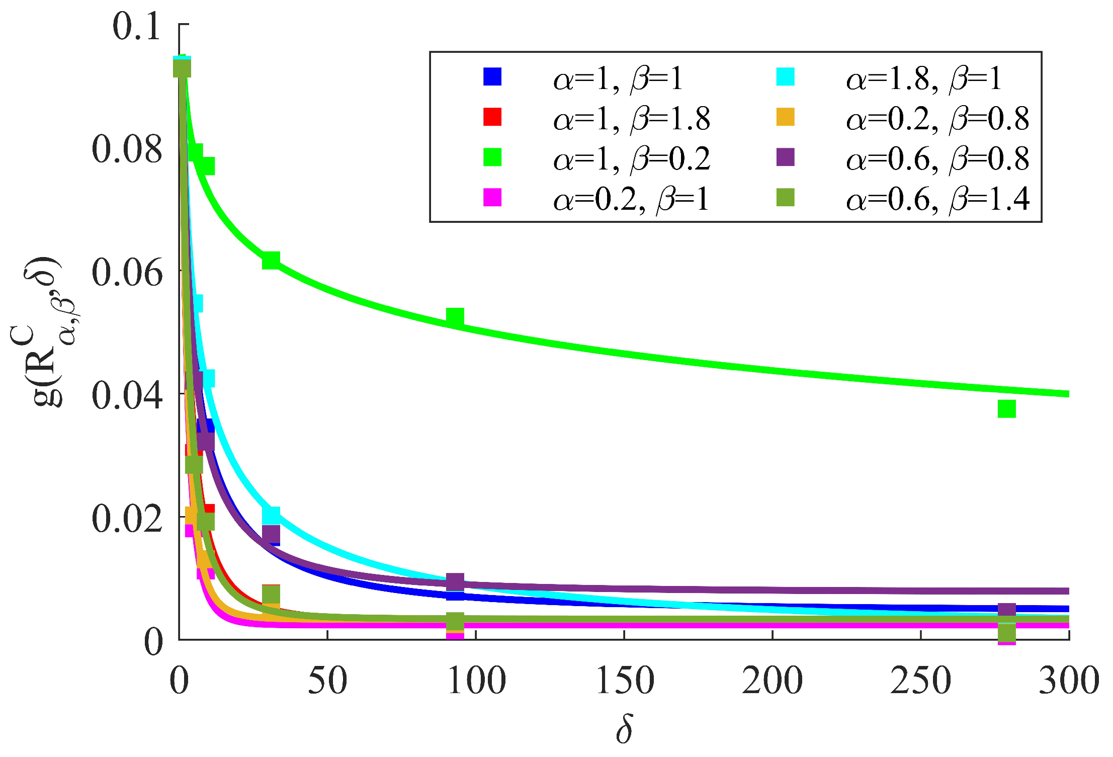
3.1. Cauchy Random Field Responses

The mesoscale apparent shear modulus responses for the case of Cauchy random fields are shown in Figure 2. It can be observed that for all ( α , β , δ ) , the inequalities of Equation (10) are satisfied. The mesoscale, δ , at which the values of c δ d and c δ n approximately converge is within the range of δ values considered for all ( α , β ) , except for when ( α = 1 , β = 0.2 ) . For the cases with α = 1 and varying β , the δ at which convergence occurred increased as the β value decreased. For the case with β = 1 and varying α , the δ values at which convergence occurred for the cases with α = 1 and α = 1.8 are similar and are far greater than that for the case with α = 0.2 . Note that a higher α indicates a lower fractal dimension and a higher β indicates a lower Hurst parameter and vice versa. These results qualitatively suggest that the δ at which convergence occurs increases as the Hurst parameter increases. Similarly, the δ at which convergence occurs increases as the fractal dimension decreases.
In order to quantitatively understand these results, the scaling data are plotted for all combinations of ( α , β ) , along with the corresponding stretched exponential fits and the Cauchy function fits in Figure 3 and Figure 4, respectively. The coefficients, A, B, and C, of the stretched exponential fits for the scaling data, are given in Table 1a. The higher B’s value is, the quicker is the convergence, and the above-mentioned qualitative inferences are in line with the change in B value with ( α , β ) . The coefficients of Cauchy function fits, A C , B C , and C C , are also given in Table 1a for reference. The residual error comparison between the stretched exponential fit and the Cauchy function fit shows that the Cauchy function fit is better than the stretched exponential fit in five out of the eight cases.

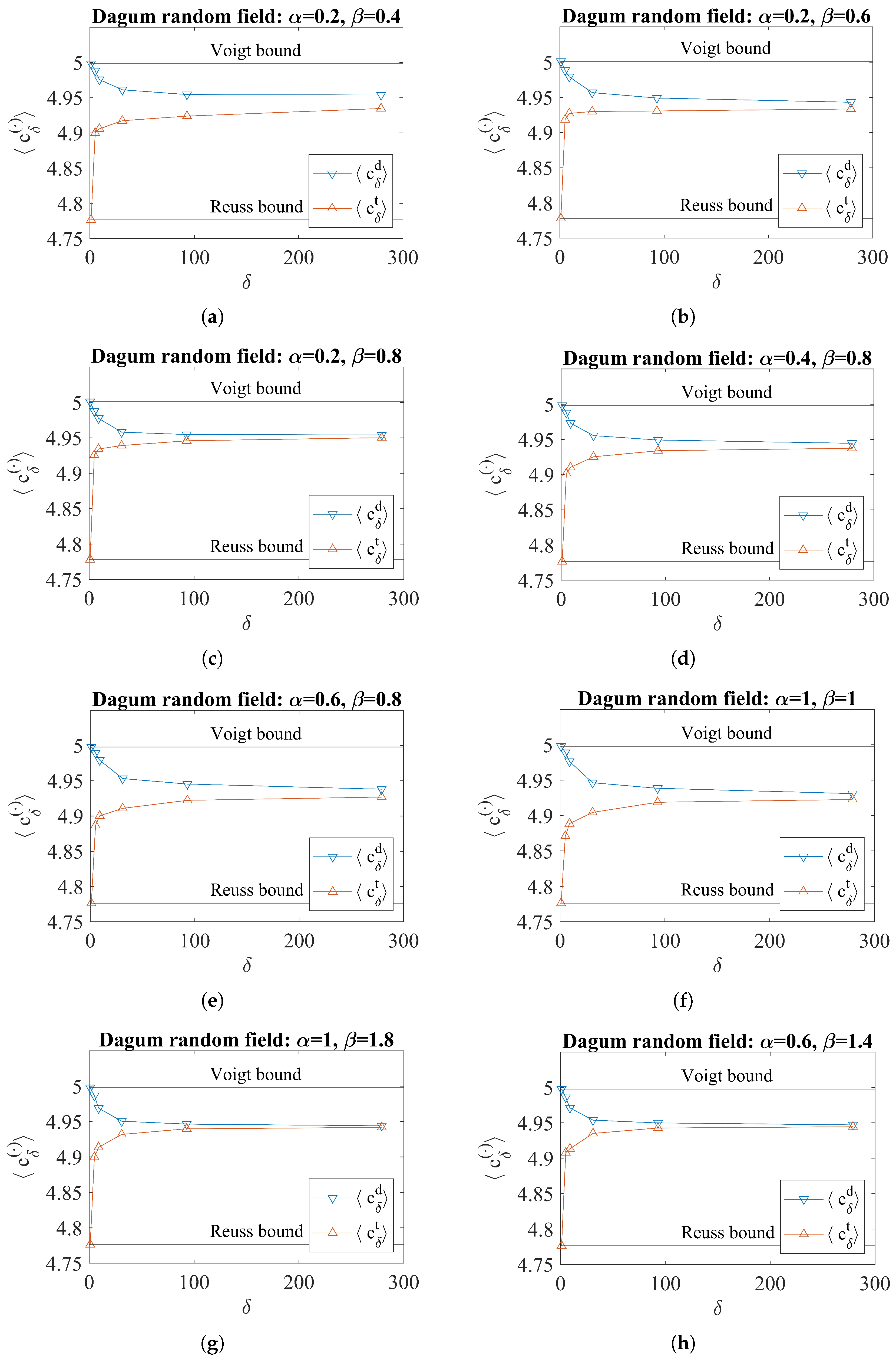
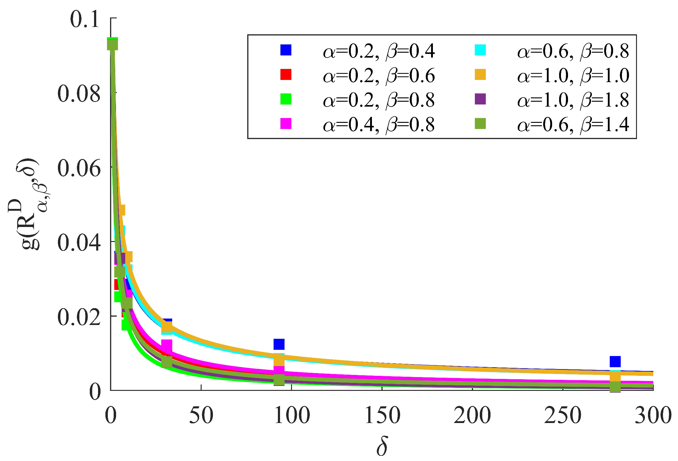
3.2. Dagum Random Field Responses

The mesoscale apparent shear modulus responses for the case of Dagum random fields are shown in Figure 5. It can be observed that for all ( α , β , δ ) , the inequalities of Equation (10) are satisfied. Convergence occurs within the range of δ values considered for all ( α , β ) . For the cases with α = 0.2 and varying β , the rate of convergence with respect to δ is higher for the case with a larger β value. For the case with β = 0.8 and varying α , the rate of convergence with respect to δ is higher for the case with a smaller α value. Analogously to the case of Cauchy random fields, the Dagum random field results qualitatively suggest that a larger β and a smaller α indicate a higher rate of convergence with respect to δ . The scaling data are plotted for all combinations of ( α , β ) , along with the corresponding stretched exponential fits and the Dagum function fits in Figure 6 and Figure 7, respectively. The coefficients, A, B, and C, of the stretched exponential fits for the scaling data, are given in Table 1b. The above-mentioned qualitative inferences are in line with the change in B value with ( α , β ) . The coefficients of Dagum function fits, A D , B D , and C D are also given in Table 1b for reference. The residual error comparison between the stretched exponential fit and the Dagum function fit shows that the Dagum function fit is better than the stretched exponential fit in five out of the eight cases.
Five out of the eleven combinations of ( α , β ) are common in Cauchy and Dagum random fields considered in the current study (see Table 1). It can be observed that for each ( α , β ) , the convergence is a bit quicker for the corresponding Cauchy random field response than that of the Dagum random field response, which is evident from the B values given in Table 1. However, note that for the same α , β , the differences between the Cauchy random field response and the Dagum random field response are not very different. These results suggest that the random shear modulus fields having a particular ( D , H ) may be modeled either by Cauchy or Dagum random fields without significant difference in the anti-plane response.

4. Conclusions

In this article, the length scale effect on the apparent shear modulus values within the context dictated by the Hill–Mandel macrohomogeneity condition was studied. The effective shear modulus for a random microstructure was bounded above and below by the apparent responses of stochastic boundary value problems under uniform displacement and the uniform traction boundary conditions, respectively. The microstructural randomness was introduced through Cauchy and Dagum stochastic models which can both capture and separate fractal and Hurst effects. A varied set of ( α , β ) in both Cauchy and Dagum random fields were studied at each mesoscale δ . A physics-based cellular automaton was used to obtain the apparent shear modulus responses of the stochastic boundary value problems for all ( α , β , δ ). Major results include:
(i) The obtained scaling data show that the mesoscale δ at which the effective shear modulus response is strongly dependent on the choice of parameters varies with α and β .
(ii) It was found that for a fixed α , the rate of convergence with respect to δ increases with an increase in β . For a fixed β , the rate of convergence with respect to δ increases with a decrease in α .
(iii) The scaling data of the corresponding Cauchy and Dagum random field responses were found to be approximated better by Cauchy-type and Dagum-type functions, respectively, than by a stretched exponential function which works very well in white-noise-type random media.
The methodology of the current work can be extended to study the scale-dependent bounds in media represented by tensor random fields without assuming local isotropy.

Author Contributions

Conceptualization, M.O.-S.; methodology, Y.S.J. and M.O.-S.; software, Y.S.J.; validation, Y.S.J.; formal analysis, Y.S.J. and M.O.-S.; investigation, M.O.-S.; resources, Y.S.J. and M.O.-S.; data curation, Y.S.J.; writing—original draft preparation, Y.S.J.; writing—review and editing, Y.S.J. and M.O.-S.; visualization, Y.S.J.; supervision, M.O.-S.; project administration, M.O.-S.; funding acquisition, M.O.-S. All authors have read and agreed to the published version of the manuscript.

Funding

This research received no external funding.

Institutional Review Board Statement

Not applicable.

Informed Consent Statement

Not applicable.

Data Availability Statement

All data are shown clearly in the plots and tables, and will be made available up on reasonable request.

Acknowledgments

We thank Emilio Porcu and Francisco Cuevas for helpful suggestions on the generation of random fields. We also thank Xian Zhang and Vinesh Nishawala for their prior work on this project.

Conflicts of Interest

The authors declare no conflict of interest.

References

  1. Ostoja-Starzewski, M. Microstructural Randomness and Scaling in Mechanics of Materials; Chapman and Hall/CRC: Boca Raton, FL, USA, 2007. [Google Scholar]
  2. Ostoja-Starzewski, M.; Kale, S.; Karimi, P.; Malyarenko, A.; Raghavan, B.; Ranganathan, S.; Zhang, J. Scaling to RVE in random media. Adv. Appl. Mech. 2016, 49, 111–211. [Google Scholar]
  3. Huet, C. Application of variational concepts to size effects in elastic heterogeneous bodies. J. Mech. Phys. Solids 1990, 38, 813–841. [Google Scholar] [CrossRef]
  4. Sab, K. On the homogenization and the simulation of random materials. Eur. J. Mech. Solids 1992, 11, 585–607. [Google Scholar]
  5. Ranganathan, S.I.; Ostoja-Starzewski, M. Scaling function, anisotropy and the size of RVE in elastic random polycrystals. J. Mech. Phys. Solids 2008, 56, 2773–2791. [Google Scholar] [CrossRef]
  6. Ranganathan, S.I.; Ostoja-Starzewski, M. Towards scaling laws in random polycrystals. Int. J. Eng. Sci. 2009, 47, 1322–1330. [Google Scholar] [CrossRef]
  7. Murshed, M.R.; Ranganathan, S.I. Hill–Mandel condition and bounds on lower symmetry elastic crystals. Mech. Res. Commun. 2017, 81, 7–10. [Google Scholar] [CrossRef]
  8. Dalaq, A.S.; Ranganathan, S.I. Invariants of mesoscale thermal conductivity and resistivity tensors in random checkerboards. Eng. Comput. 2015, 32, 1601–1618. [Google Scholar] [CrossRef]
  9. Kale, S.; Saharan, A.; Koric, S.; Ostoja-Starzewski, M. Scaling and bounds in thermal conductivity of planar Gaussian correlated microstructures. J. Appl. Phys. 2015, 117, 104301. [Google Scholar] [CrossRef]
  10. Ostoja-Starzewski, M.; Schulte, J. Bounding of effective thermal conductivities of multiscale materials by essential and natural boundary conditions. Phys. Rev. B 1996, 54, 278. [Google Scholar] [CrossRef] [Green Version]
  11. Ghossein, E.; Lévesque, M. Homogenization models for predicting local field statistics in ellipsoidal particles reinforced composites: Comparisons and validations. Int. J. Solids Struct. 2015, 58, 91–105. [Google Scholar] [CrossRef]
  12. Savvas, D.; Stefanou, G.; Papadrakakis, M. Determination of RVE size for random composites with local volume fraction variation. Comput. Methods Appl. Mech. Eng. 2016, 305, 340–358. [Google Scholar] [CrossRef]
  13. Raghavan, B.V.; Ranganathan, S.I.; Ostoja-Starzewski, M. Electrical properties of random checkerboards at finite scales. AIP Adv. 2015, 5, 017131. [Google Scholar] [CrossRef] [Green Version]
  14. Karimi, P.; Zhang, X.; Yan, S.; Ostoja-Starzewski, M.; Jin, J.M. Electrostatic and magnetostatic properties of random materials. Phys. Rev. E 2019, 99, 022120. [Google Scholar] [CrossRef] [Green Version]
  15. Mandelbrot, B. The Fractal Geometry of Nature; W.H. Freeman & Co.: New York, NY, USA, 1982. [Google Scholar]
  16. Malyarenko, A.; Ostoja-Starzewski, M. Tensor-Valued Random Fields for Continuum Physics; Cambridge University Press: Cambridge, UK, 2019. [Google Scholar]
  17. Hill, R. Elastic properties of reinforced solids: Some theoretical principles. J. Mech. Phys. Solids 1963, 11, 357–372. [Google Scholar] [CrossRef]
  18. Mandel, J.; Dantu, P. Contribution à l’étude théorique et expérimentale du coefficient d’élastcité d’un milieu hétérogène, mais statistiquement homogène. Annales des Ponts et Chaussées Paris 1963, 6, 115–145. [Google Scholar]
  19. Hill, R. The Mathematical Theory of Plasticity; Oxford University Press: Oxford, UK, 1998; Volume 11. [Google Scholar]
  20. Gneiting, T.; Schlather, M. Stochastic models that separate fractal dimension and the Hurst effect. SIAM Rev. 2004, 46, 269–282. [Google Scholar] [CrossRef] [Green Version]
  21. Porcu, E. Spatio-Temporal Geostatistics: New Classes of Covariance, Variogram and Spectral Densities. Ph.D. Thesis, University of Milano, Milano, Italy, 2004. [Google Scholar]
  22. Chiles, J.P.; Delfiner, P. Geostatistics: Modeling Spatial Uncertainty; John Wiley & Sons: Hoboken, NJ, USA, 2009. [Google Scholar]
  23. Porcu, E.; Mateu, J.; Zini, A.; Pini, R. Modelling spatio-temporal data: A new variogram and covariance structure proposal. Stat. Probab. Lett. 2007, 77, 83–89. [Google Scholar] [CrossRef]
  24. Lim, S.; Teo, L. Analytic and asymptotic properties of multivariate generalized Linnik’s probability densities. J. Fourier Anal. Appl. 2010, 16, 715–747. [Google Scholar] [CrossRef] [Green Version]
  25. Laudani, R.; Zhang, D.; Faouzi, T.; Porcu, E.; Ostoja-Starzewski, M.; Chamorro, L.P. On streamwise velocity spectra models with fractal and long-memory effects. Phys. Fluids 2021, 33, 035116. [Google Scholar] [CrossRef]
  26. Davies, T.M.; Bryant, D. On circulant embedding for Gaussian random fields in R. J. Stat. Softw. 2013, 55, 1–21. [Google Scholar] [CrossRef] [Green Version]
  27. von Neumann, J.; Burks, A.W. Theory of Self-Reproducing Automata; University of Illinois Press Urbana: Champaign, IL, USA, 1966; Volume 1102024. [Google Scholar]
  28. Leamy, M.J. Application of cellular automata modeling to seismic elastodynamics. Int. J. Solids Struct. 2008, 45, 4835–4849. [Google Scholar] [CrossRef] [Green Version]
  29. Hopman, R.K.; Leamy, M.J. Arbitrary geometry cellular automata for elastodynamics. In Proceedings of the ASME International Mechanical Engineering Congress and Exposition, Lake Buena Vista, FL, USA, 13–19 November 2009; Volume 43888, pp. 535–547. [Google Scholar]
  30. Zhang, X.; Nishawala, V.; Ostoja-Starzewski, M. Anti-plane shear Lamb’s problem on random mass density fields with fractal and Hurst effects. Evol. Equ. Control Theory 2019, 8, 231. [Google Scholar] [CrossRef] [Green Version]
Figure 1. (a) A cell (i,j) and its von Neumann neighbours for cellular automaton discretization. (b) neighbor forces and the external force acting on cell (i,j).
Fractalfract 05 00255 g001
Figure 2. Apparent shear modulus responses corresponding to Cauchy random fields for various combinations of ( α , β , δ ) .
Fractalfract 05 00255 g002
Figure 3. The scaling function g ( R α , β C , δ ) as a function of δ and the corresponding stretched exponential fit.
Fractalfract 05 00255 g003
Figure 4. The scaling function g ( R α , β C , δ ) as a function of δ and the corresponding Cauchy function fit.
Fractalfract 05 00255 g004
Figure 5. Apparent shear modulus responses corresponding to Dagum random fields for various combinations of ( α , β , δ ) .
Fractalfract 05 00255 g005
Figure 6. The scaling function g ( R α , β D , δ ) as a function of δ and the corresponding stretched exponential fit.
Fractalfract 05 00255 g006
Figure 7. The scaling function g ( R α , β D , δ ) as a function of δ and the corresponding Dagum function fit.
Fractalfract 05 00255 g007
Table 1. Different combinations of α and β in Cauchy and Dagum random fields. (A, B, C), ( A C , B C , C C ), and ( A D , B D , C D ) are the coefficients in the stretched exponential, the Cauchy function, and the Dagum function, respectively. S S E , S S E C , and S S E D are the error sums of the squares corresponding to the stretched exponential and Cauchy and Dagum functions’ fits, respectively.
α β DHABC S S E A C B C C C S S E C
112.50.50.240.340.0052.5 × 10 6 0.460.342.32.1 × 10 6
11.82.50.10.240.460.0032.2 × 10 5 0.114.600.161 × 10 6
10.22.50.90.500.05−0.0902.7 × 10 5 0.120.530.353.9 × 10 5
0.212.90.50.250.600.0023.7 × 10 6 25.360.228.117.5 × 10 6
1.812.10.50.250.270.0019.4 × 10 7 0.170.690.822.7 × 10 5
0.20.82.90.60.240.580.0032.2 × 10 5 14.880.237.331.2 × 10 5
0.60.82.70.60.230.370.0082.8 × 10 5 1.110.233.595.6 × 10 6
0.61.42.70.30.240.480.0042.4 × 10 5 1.900.294.361.4 × 10 5
(a) Cauchy random fields
α β DHABC S S E A D B D C D S S E D
0.20.42.90.80.220.450.0124.9 × 10 5 2.350.580.0568.5 × 10 5
0.20.62.90.70.230.510.0073.7 × 10 5 2.430.750.0556.5 × 10 6
0.20.82.90.60.240.520.0043.3 × 10 5 0.760.900.1872.3 × 10 5
0.40.82.80.60.240.420.0063.1 × 10 5 0.540.750.2738.7 × 10 6
0.60.82.70.60.230.360.0062.1 × 10 5 0.660.600.2154.5 × 10 6
112.50.50.240.320.0043.3 × 10 6 0.220.640.8214.9 × 10 6
11.82.50.10.250.420.0026.4 × 10 6 0.150.951.335.8 × 10 8
0.61.42.70.30.240.440.0032.6 × 10 5 1.180.810.1196.3 × 10 6
(b) Dagum random fields
Publisher’s Note: MDPI stays neutral with regard to jurisdictional claims in published maps and institutional affiliations.

