Numerical Solutions of a Heat Transfer for Fractional Maxwell Fluid Flow with Water Based Clay Nanoparticles; A Finite Difference Approach

Abstract

Fractional-order mathematical modelling of physical phenomena is a hot topic among various researchers due to its many advantages over positive integer mathematical modelling. In this context, the appropriate solutions of such fractional-order physical modelling become a challenging task among scientists. This paper presents a study of unsteady free convection fluid flow and heat transfer of Maxwell fluids with the presence of Clay nanoparticle modelling using fractional calculus. The obtained model was transformed into a set of linear nondimensional, partial differential equations (PDEs). The finite difference scheme is proposed to discretize the obtained set of nondimensional PDEs. The Maple code was developed and executed against the physical parameters and fractional-order parameter to explain the behavior of the velocity and temperature profiles. Some limiting solutions were obtained and compared with the latest existing ones in literature. The comparative study witnesses that the proposed scheme is a very efficient tool to handle such a physical model and can be extended to other diversified problems of a complex nature.

1. Introduction

Many physical phenomena of the natural sciences can be illustrated by differential equations with suitable initial and boundary conditions such as the flow of Maxwell fluids. Researchers commonly focus on the cases where the governing equations represent Newtonian and other non-Newtonian behaviors of fluids. Whereas, during the last decades, researchers have been interested in mathematical models involving Maxwell fluid flow. Because of the simplicity of the Maxwell model, it is widely used, especially to describe the response of some polymeric liquids.

On the other hand, this model also has some limitations such as the description of the relation between shear stress and shear strain which is absent in this model [1,2,3,4,5,6,7]. As the Maxwell fluids are non-Newtonian, time dependent, and viscoelastic fluids, the heat and mass transfer of Maxwell fluids is considered an important issue that is consequently challenging for researchers. By the change in flow geometry and boundary conditions, the heat flow characteristics through any system can be enhanced. For this purpose, many techniques have been developed to enhance the heat transfer characteristics of fluids. Researchers have also tried to improve the thermal conductivity of base fluids by suspending the micro- or larger-sized solid particles in fluids, since the thermal conductivity of a solid is typically greater than that of liquids. So, it was not very useful for any system where the settling of solid particles of suspension occur, because of the large size and high density level of the particles [8].

Entropy generation and its solution are considered a major concern for industrialists in recent times. Viscous dissipation, heat flow, mass flow, and chemical reactions are known as entropy generation [9,10,11,12,13]. The entropy generation in magnetohydrodynamics (MHD) has also been investigated analytically [14]. MHD effects on flow, entropy generation and role of the Bejan number have been investigated by Awad [15,16]. To overcome the problem, Choi gave the idea of nanofluids [17]. Nanofluids are composed of nanometer-sized solid particles, rods or tubes comprised of solid and liquid materials which are suspended in different base fluids. They provide a solution for enhancing heat transfer. This property improves the stability and thermal conductivity of base fluids as compared to conventional fluids. By this virtue, the nanofluids can flow more smoothly in a system without clogging.

The study of the drilling process with nanofluids is significant in the drilling methods of oil and gases from rocks, land, and oceans. For better performance of the drilling fluid, clay nanoparticles play a vital role. The addition of clay nanoparticles in drilling base fluids enhances the boiling point of the fluids, thermal conductivity, and viscosity levels which provide resistance to high temperature and control the fluid cost [18]. As there exist two ways of drilling mud: oil-based mud (OBM) and water-base mud (WBM), polymeric nanoparticles and clay nanoparticles are very useful. Clay nanoparticles help in maintaining the stability of temperature, the prevention of fluid loss, and the least value of torque, to control the rheological possession for scrubbing the hole in order to filter the quality of coke. Water, kerosene and engine oil are used for water drilling [19].

In the above-discussed reference, the classical definition of derivative is involved, which gives some particular solutions with the absence of heat transfer solutions. However, heat transfer has various commercial and industrial applications such as plastic film manufacturing, fiber coating and artificial fiber, and other chemical processing tools [20,21,22,23]. As a result, it is a main interest of researchers to give a new direction to novel fractional modeling rather than that of a classical study of the positive integer order of PDEs, as it gives a generalized result by various fractional differentiation operators [24,25,26] (See also [27]).

The solution of such physical problems with analytical techniques of a modified Laplace transformation accompanied with Adomian decomposition method is obtained [28].

Our main purpose is to extend the idea in which analytical solutions are obtained for viscous fluid. Because the research work which has already been done in this field has various gaps, such as the analytical techniques that are widely used to obtain exact solutions even though it was done after many assumptions to make the simplest model. The analytical approach of Laplace transform has been used to investigate the solution for temperature and velocity field, Imran et al. [29]. However, numerical approaches are more accurate for obtaining solutions, especially for the fractional modeling of physical phenomena, than other approaches. Therefore, we focus on the numerical solution of this problem by the finite difference scheme. The model is formulated by PDEs of integer order. We know that fractional models are superior in narrating the decay properties of field variables, therefore, we changed the integer order to a noninteger order. A differentiation operator of Caputo is applied to formulate the model. A finite difference scheme is proposed to discretize the obtained set of nondimensional PDEs. Thermo-physical properties of various nanoparticles are given in

Table 1. Various material with different thermos-physio properties [30].

Material	Symbol	$\mathit{\rho }$	${\mathit{c}}_{\mathit{p}}$	K	$\mathit{\beta }$	Pr
Clay	Nanoparticles	6320	531.8	76.5	1.8	-
Water	${\mathrm{H}}_2\mathrm{O}$	997	4179	0.613	21	6.2
Kerosene oil	KO	783	2090	0.145	99	21
Engine oil	EO	884	1910	0.114	70	500

.

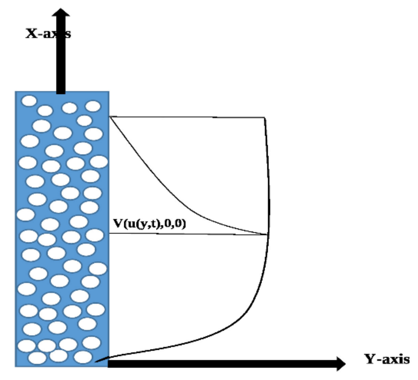
2. Formulation and Mathematical Modeling

Considering three base fluids (water, kerosene oil and engine oil) that have been added to the flow of clay nanoparticles, assume that the flow is 1-dimensional and 1-directional along $y>0$ direction i.e., velocity profile is $V\left(x,y,z,t\right)=\left[u\left(y,t\right), 0,0\right]$. The nanofluid is close to a heated vertical and infinite plate. Initially the temperature is ${\Theta }_{\infty }$ in the surrounding of this stationary infinite plate. This physical phenomena is illustrated in the following Figure 1.

As the temperature rises from ${\Theta }_{\infty }$ to ${\Theta }_w$ which results in moving the plate with velocity $V_0$ forcing the fluids in $y$-direction.

So, continuity equation (CE) [31] is,

$$\frac{\partial \rho }{\partial t}+\rho \left(\nabla V\right)=0.$$

where $\rho$ dynamic viscosity, $\nabla$ is the gradient operator, with $V$ a velocity field. However, for the fluids which are incompressible, continuity equation (CE) becomes

$$\nabla V=0.$$

The tensor form of Maxwell fluid is given by [32],

$$T=-pI+S,$$

where $S+{\lambda }_1\frac{DS}{Dt}=\mu A_1.$

The Cauchy stress tensor, pressure gradient, identity matrix tensor, extra stress tensor, dynamic viscosity and Rivlin Erikson tensor are represented by $T,p,S,\mu \mathrm{and}{A}_1\mathrm{respectively}.$ In the above expression:

$$A_1=\nabla V+{(\nabla V)}^T,$$

$$\frac{DS}{Dt}=\frac{\partial S}{\partial t}-SL-S{L}^T,$$

where $\frac{D}{Dt}$ is the material time derivative (the sum of local and convective (nonlocal) part), and $L$ is the velocity gradient.

The generalized Maxwell fluid can be represented in tensor form with Caputo time fractional differentiation operator as [18]:

$$\left(1+{\lambda }_1^{\alpha }\frac{{\partial }^{\alpha }}{\partial t^{\alpha }}\right)\tau ={\mu }_{nf}\frac{\partial v}{\partial y},$$

where $\tau =S_{xy}$ is the component of extra stress tensor, which is non-zero and $\frac{{\partial }^{\alpha }}{\partial t^{\alpha }}={}_0{}^{C}D{}_t^{\alpha }$ Caputo time fractional differentiation operator with the fractional parameter $\alpha$. Defined as [33]:

$${}_0{}^{C}D{}_t^{\alpha }f\left(t\right)=\frac{1}{\Gamma \left(1-\alpha \right)}{{\displaystyle \int }}_0^t{\left(t-n\right)}^{-\alpha }\frac{\partial f\left(\eta \right)}{\partial \eta }d\eta , 0<\alpha <1,$$

and $\Gamma \left(.\right)$ is the Gamma function defined by [33]

$$\Gamma \left(z\right)=\int {\eta }^{z-1}{e}^{-\eta }, zϵℂ, ℝe\left(z\right)˃0.$$

Since the flow is incompressible, non-Newtonian viscoelastic, 1-dimensional and Uni-directional. Therefore, the governing equations of momentum and energy presented in [18,19,34] after applying Caputo time derivative, in the absence of pressure gradient and convective term, take the following form:

$$\begin{gathered} {\rho }_{nf}\left(1+{\lambda }_1^{\alpha } \frac{{\partial }^{\alpha }}{\partial t^{\alpha }}\right)\frac{\partial u\left(y, t\right)}{\partial t}={\mu }_{nf}\frac{{\partial }^{2}u\left(y,t\right)}{\partial y^2}+\left(1+{\lambda }_1^{\alpha } \frac{{\partial }^{\alpha }}{\partial t^{\alpha }}\right)g{\left(\rho {\beta }_{\Theta }\right)}_{nf} \\ \times \left(\Theta \left(y,t\right)-{\Theta }_{\infty }\right), \end{gathered}$$

(1)

$${\left(\rho C_p\right)}_{nf}\frac{\partial \Theta \left(y,t\right)}{\partial t}=-\frac{\partial q\left(y,t\right)}{\partial y}.$$

(2)

By applying the Maxwell parameter $\left(1+{\lambda }_2^{\beta }\frac{{\partial }^{\beta }}{\partial t^{\beta }}\right)$ on both sides of Equation (2) for fractional energy equation [34,35].

$${\left(\rho C_p\right)}_{nf}\left(1+{\lambda }_2^{\beta } \frac{{\partial }^{\beta }}{\partial t^{\beta }}\right)\frac{\partial \Theta \left(y,t\right)}{\partial t}=-\frac{\partial }{\partial y}\left(1+{\lambda }_2^{\beta } \frac{{\partial }^{\beta }}{\partial t^{\beta }}\right)q$$

(3)

However, generalization of fractional Cattaneo’s law [36].

$$\left(1+{\lambda }_{\beta } \frac{{\partial }^{\beta }}{\partial t^{\beta }}\right)q=K_{nf}\frac{\partial \Theta \left(y,t\right)}{\partial y}.$$

(4)

Therefore, the Equation (2), becomes

$${\left(\rho C_p\right)}_{nf}\left(1+{\lambda }_2^{\beta } \frac{{\partial }^{\beta }}{\partial t^{\beta }}\right)\frac{\partial \Theta \left(y,t\right)}{\partial t}=K_{nf}\frac{{\partial }^2\Theta \left(y,t\right)}{\partial y^2},$$

(5)

where the initial and boundary conditions are:

$$u\left(0,t\right)=0, \Theta \left(0,t\right)={\Theta }_{\infty }, \forall y\ge 0,$$

(6)

$$u\left(y,t\right)=V_{0}H\left(t\right), \Theta \left(0,t\right)={\Theta }_w for t>0,$$

(7)

$$u\left(\infty ,t\right)\to 0,\Theta \left(\infty ,t\right)\to {\Theta }_{\infty } for t>0.$$

(8)

where $H\left(t\right)$ is Heaviside unit step function. The thermo-physical properties are as follows [30]:

$$\frac{{\rho }_{nf}-\varphi {\rho }_s}{\left(1-\varphi \right){\rho }_f}=1, \frac{{\mu }_{nf}}{{\mu }_f}{\left(1-\varphi \right)}^{2.5}=1,\frac{ {\left(\rho C_p\right)}_{nf}-\varphi {\left(\rho C_p\right)}_s}{\left(1-\varphi \right){\left(\rho C_p\right)}_f}=1,$$

(9)

$$\frac{K_{nf}}{K_f}=\frac{K_s+2K_f-2\varphi \left(K_f-K_s\right)}{K_s+2K_f+2\varphi \left(K_f-K_s\right)}, \frac{{\left(\rho {\beta }_{\Theta }\right)}_{nf}-\varphi {\left(\rho {\beta }_{\Theta }\right)}_s)}{\left(1-\varphi \right){\left(\rho {\beta }_{\Theta }\right)}_f}=1.$$

(10)

Some nondimensional parameters and functions are used to make Equations (1) and (5) dimensionless:

$$y^{*}=\frac{V_0}{{\nu }_f}y, t^{*}=\frac{V_0^2}{V_f}t, {\theta }^{*}=\frac{\Theta -{\Theta }_{\infty } }{{\Theta }_w-{\Theta }_{\infty }}, u^{*}=\frac{u}{V_0}.$$

(11)

Applying these nondimensional parameters, relations in Equations (9) and (10) and removing the ($\ast$) notation of nondimensional parameters, the Equations (1) and (5) become:

$$b_0\left(1+{\lambda }_1\frac{{\partial }^{\alpha }}{\partial t^{\alpha }}\right)\frac{\partial u\left(y,t\right)}{\partial t}=b_1\frac{{\partial }^{2}u\left(y,t\right)}{\partial t^2}+b_{2}Gr\left(1+{\lambda }_1\frac{{\partial }^{\alpha }}{\partial t^{\alpha }}\right)\theta \left(y,t\right),$$

(12)

$$\left(1+{\lambda }_2\frac{{\partial }^{\beta }}{\partial t^{\beta }}\right)\frac{\partial \Theta \left(y,t\right)}{\partial t}=b_5 \frac{{\partial }^2\theta \left(y,t\right)}{\partial y^2}.$$

(13)

Similarly, using nondimensional parameters the boundary conditions are as follows:

$$u\left(0,t\right)=0, \theta \left(0,t\right)=0 \forall y\ge 0,$$

(14)

$$u\left(0,t\right)=H\left(t\right), \theta \left(0,t\right)=1 \mathit{for} t>0,$$

(15)

$$u\left(y,t\right)\to 0, \theta \left(y,t\right)\to 0 \mathit{as} y\to \infty \mathit{for} t>0.$$

(16)

In these expressions, the $b_0,b_1,b_3,b_4$ and $b_5$ are given as:

$$b_0=\left\{\left(1-\varphi \right)+\frac{{\rho }_s}{{\rho }_f}\right\},b_1=\left\{\frac{1}{{\left(1-\varphi \right)}^{2.5}}\right\}, b_2=\left\{\left(1-\varphi \right)+\varphi \frac{{\left(\rho {\beta }_{\Theta }\right)}_s}{{\left(\rho {\beta }_{\Theta }\right)}_f}\right\},$$

$$b_3=\left\{\left(1-\varphi \right)+\varphi \frac{{\left(\rho C_p\right)}_s}{{\left(\rho C_p\right)}_f}\right\}, b_4=\frac{K_{nf}}{K_f}, \mathit{and} b_5=\frac{b_4}{b_{3}Pr}$$

$${\lambda }_1={\lambda }_{1\alpha }\frac{V_0^2}{v_f}, Pr=\frac{{\left(\mu C_p\right)}_f}{K_f} \mathit{and} Gr=\frac{g{v}_f{\left({\beta }_{\Theta }\right)}_f\left({\Theta }_w-{\Theta }_{ }{}_{\infty }\right)}{V_0^3}, {\lambda }_2={\lambda }_{1\beta }\frac{V_0^2}{v_f}$$

where $\alpha ,\beta$ are noninteger fractional parameters involved in $\frac{{\partial }^{\alpha }}{\partial t^{\alpha }}$ and $\frac{{\partial }^{\beta }}{\partial t^{\beta }}$ which are Caputo time differential operators [37,38].

3. Numerical Procedure

Since the finite difference discretization of fractional-order derivative of ${}_0{}^{C}D{}_t^{\alpha }u,{}_0{}^{C}D{}_t^{1+\alpha }u$ for $0<\alpha \le 1,u_t$ and $u_{yy}$ is given as Equations (12) and (13).

$${}_0{}^{C}D{}_{t_{j+1}}^{\alpha }u\left(x_i,t_{j+1}\right)=\frac{2^{-1}\mathsf{\Delta }{t}^{-\alpha }}{\Gamma \left(2-\alpha \right)}\left[u_i^{j+1}-u_i^{j-1}\right]+\frac{2^{-1}\mathsf{\Delta }{t}^{-\alpha }}{\Gamma \left(2-\alpha \right)}{\displaystyle \sum }_{l=1}^j\left(u_i^{j-l+1}-u_i^{j-l}\right)b_l^{\alpha },$$

(17)

$$\begin{gathered} {}_0{}^{C}D{}_{t_{j+1}}^{1+\alpha }u\left(x_i,t_{j+1}\right)=\frac{\mathsf{\Delta }{t}^{-\left(1+\alpha \right)}}{\Gamma \left(2-\alpha \right)}\left[u_i^{j+1}-2u_i^j+u_i^{j-1}\right]+\frac{\mathsf{\Delta }{t}^{-\left(1+\alpha \right)}}{\Gamma \left(2-\alpha \right)} \\ \times {\displaystyle \sum }_{l=1}^j\left(u_i^{j-l+1}-2u_i^{j-l}+u_i^{j-l-1}\right)b_l^{\alpha }, \end{gathered}$$

(18)

$${\left.\frac{\partial }{\partial t}u\left(x_i,t_{j+1}\right)\right|}_{t=t_{j+1}}=\frac{1}{2\mathsf{\Delta }t}\left[u_i^{j+1}-u_i^{j-1}\right],$$

(19)

$${\left.\frac{{\partial }^2}{\partial y^2}u\left(x_{i+1},t_j\right)\right|}_{x=x_{i+1}}=\frac{1}{\mathsf{\Delta }{x}^2}\left[u_{i+1}^{j+1}-2u_i^{j+1}+u_{i-1}^{j+1}\right].$$

(20)

In Equations (17) and (18), $b_l^{\alpha }={\left(l+1\right)}^{1-\alpha }-l^{1-\alpha }$ for $l=1,2,3,\dots ,j.$ Rectilinear grid deliberated for the numerical solution of discussed problem with grid spacing $\mathsf{\Delta }t>0$ and $\mathsf{\Delta }x>0$ in time and space coordinate directions individually, where $\mathsf{\Delta }x=L/M$ and $\mathsf{\Delta }t=T/N$ with $\mathsf{\Delta }x,\mathsf{\Delta }t\in {\mathbb{Z}}^{+}$. The interior points $\left(x_i,t_j\right)$ in the domain $\Omega =\left[0,T\right]\times \left[0,L\right]$ are defined as $x_i=i\Delta x$ and $t_j=j\mathsf{\Delta }t$. The discretization of above discussed model Equations (12) and (13) at each internal grid point $\left(i,j\right)$ is given as:

$$\begin{gathered} \frac{b_0}{2\mathsf{\Delta }t}\left(u_i^{j+1}-u_i^{j-1}\right)+\frac{{\theta }_{\alpha }\mathsf{\Delta }{t}^{-\left(1+\alpha \right)}}{\Gamma \left(2-\alpha \right)}\left(u_i^{j+1}-2u_i^j+u_i^{j-1}\right)+\frac{{\theta }_{\alpha }\mathsf{\Delta }{t}^{-\left(1+\alpha \right)}}{\Gamma \left(2-\alpha \right)} \\ \times {\displaystyle \sum }_{l=1}^j\left(u_i^{j-l+1}-2u_i^{j-l}+u_i^{j-l-1}\right)b_l^{\alpha }=\frac{b_1}{\mathsf{\Delta }{x}^2}\left(u_{i+1}^{j+1}-2u_i^{j+1}+u_{i-1}^{j+1}\right)+b_{2}Gr{\theta }_i^{j+1} \\ +\frac{b_{2}Gr\mathsf{\Delta }{t}^{-\alpha }}{2\Gamma \left(2-\alpha \right)}\left({\theta }_i^{j+1}-{\theta }_i^{j-1}\right)+\frac{b_{2}Gr\mathsf{\Delta }{t}^{-\alpha }}{2\Gamma \left(2-\alpha \right)}{\displaystyle \sum }_{l=1}^j\left({\theta }_i^{j-l+1}-{\theta }_i^{j-l-1}\right)b_l^{\alpha }, \\ \frac{1}{2\mathsf{\Delta }t}\left({\theta }_i^{j+1}-{\theta }_i^{j-1}\right)+\frac{{\theta }_{\beta }\mathsf{\Delta }{t}^{-\left(1+\beta \right)}}{\Gamma \left(2-\beta \right)}\left({\theta }_i^{j+1}-2{\theta }_i^j+{\theta }_i^{j-1}\right) \\ +\frac{{\theta }_{\beta }\mathsf{\Delta }{t}^{-\left(1+\beta \right)}}{\Gamma \left(2-\beta \right)}{\displaystyle \sum }_{l=1}^j\left({\theta }_i^{j-l+1}-2{\theta }_i^{j-l}+{\theta }_i^{j-l-1}\right)b_l^{\beta }=\frac{b_5}{\mathsf{\Delta }{x}^2}\left({\theta }_{i+1}^{j+1}-2{\theta }_i^{j+1}+{\theta }_{i-1}^{j+1}\right). \end{gathered}$$

Assume that

$$\begin{gathered} {\omega }_1=\frac{2{\theta }_{\alpha }\mathsf{\Delta }{t}^{-\alpha }}{b_0\Gamma \left(2-\alpha \right)},r_1=2\frac{b_1}{b_0}\frac{\mathsf{\Delta }t}{\mathsf{\Delta }{x}^2},a=2\frac{b_2}{b_0}\Delta tGr,b=\frac{b_2}{b_0}\frac{Gr\mathsf{\Delta }{t}^{1-\alpha }}{\Gamma \left(2-\alpha \right)},{\omega }_2=\frac{2{\theta }_{\beta }\mathsf{\Delta }{t}^{-\beta }}{\Gamma \left(2-\beta \right)},r_2 \\ =2b_5\frac{\mathsf{\Delta }t}{\Delta x^2}, \end{gathered}$$

then the above equations take the following simplest form:

$$\begin{gathered} -r_1{u}_{i+1}^{j+1}+\left(1+{\omega }_1+2r_1\right)u_i^{j+1}-r_1{u}_{i-1}^{j+1}-\left(a+b\right){\theta }_i^{j+1}=2{\omega }_1{u}_i^j+\left(1-{\omega }_1\right)u_i^{j-1}-b{\theta }_i^{j-1} \\ -{\displaystyle \sum }_{l=1}^j{\omega }_1{b}_l^{\alpha }{u}_i^{j-l+1}+2{\displaystyle \sum }_{l=1}^j{\omega }_1{b}_l^{\alpha }{u}_i^{j-l}-{\displaystyle \sum }_{l=1}^j{\omega }_1{b}_l^{\alpha }{u}_i^{j-l-1}+{\displaystyle \sum }_{l=1}^{j}b{b}_l^{\alpha }{\theta }_i^{j-l+1}-{\displaystyle \sum }_{l=1}^{j}b{b}_l^{\alpha }{\theta }_i^{j-l-1}, \\ -r_2{\theta }_{i+1}^{j+1}+\left(1+{\omega }_2+2r_2\right){\theta }_i^{j+1}-r_2{\theta }_{i-1}^{j+1}=2{\omega }_2{\theta }_i^j+\left(1-{\omega }_2\right){\theta }_i^{j-1} \\ -{\displaystyle \sum }_{l=1}^j{\omega }_2{b}_l^{\beta }{\theta }_i^{j-l+1}+2{\displaystyle \sum }_{l=1}^j{\omega }_2{b}_l^{\beta }{\theta }_i^{j-l}-{\displaystyle \sum }_{l=1}^j{\omega }_2{b}_l^{\beta }{\theta }_i^{j-l-1}. \end{gathered}$$

For j = 0 the matrix form of the above discretized formula is given as:

$$\begin{gathered} -r_1{u}_{i+1}^1+\left(1+{\omega }_1+2r_1\right)u_i^1-r_1{u}_{i-1}^1-\left(a+b\right){\theta }_i^1=2{\omega }_1{u}_i^0+\left(1-{\omega }_1\right)u_i^{-1}-b{\theta }_i^{-1}, \\ -r_2{\theta }_{i+1}^1+\left(1+{\omega }_2+2r_2\right){\theta }_i^1-r_2{\theta }_{i+1}^1=2{\omega }_2{\theta }_i^0+\left(1-{\omega }_2\right){\theta }_i^{-1}, \end{gathered}$$

for $i=1,2,3,\dots ,M-1.$ Since $u_i^{-1}=u_i^1$ and ${\theta }_i^{-1}={\theta }_i^1$ then the above expression takes the following form:

$$\widehat{\mathit{K}}{\mathit{V}}^1=\mathit{L}{\mathit{V}}^0.$$

For $j>0,i=1,2,3,\dots ,M-1$ and using $u_i^{-1}=u_i^1$ and ${\theta }_i^{-1}={\theta }_i^1$, we obtain the following formula:

$$\begin{gathered} -r_1{u}_{i+1}^{j+1}+\left(1+{\omega }_1+2r_1\right)u_i^{j+1}-r_1{u}_{i-1}^{j+1}-\left(a+b\right){\theta }_i^{j+1}={\omega }_1\left(2-b_1^{\alpha }\right)u_i^j \\ +\left(1-{\omega }_1-{\omega }_1{b}_2^{\alpha }+2{\omega }_1{b}_1^{\alpha }\right)u_i^{j-1}+b{b}_1^{\alpha }{\theta }_i^j-b\left(1+b_2^{\alpha }\right){\theta }_i^{j-1}+{\displaystyle \sum }_{l=1}^{j-2}{c}_l^1{u}_i^{j-l-1}-{\omega }_1{b}_j^{\alpha }{u}_i^1 \\ +{\omega }_1\left(2b_j^{\alpha }-b_{j-1}^{\alpha }\right)u_i^0+{\displaystyle \sum }_{l=1}^{j-2}{c}_l^2{\theta }_i^{j-l-1}-b{b}_j^{\alpha }{\theta }_i^1-b{b}_{j-1}^{\alpha }{\theta }_i^0, \\ -r_2{\theta }_{i+1}^{j+1}+\left(1+{\omega }_2+2r_2\right){\theta }_i^{j+1}-r_2{\theta }_{i-1}^{j+1}={\omega }_2\left(2-b_1^{\beta }\right){\theta }_i^j+\left(1-{\omega }_2-{\omega }_2{b}_2^{\beta }+2{\omega }_2{b}_1^{\beta }\right){\theta }_i^{j-1} \\ +{\displaystyle \sum }_{l=1}^{j-2}{c}_l^2{\theta }_i^{j-l-1}-{\omega }_2{b}_j^{\beta }{\theta }_i^1+{\omega }_2\left(2b_j^{\beta }-b_{j-1}^{\beta }\right){\theta }_i^0. \end{gathered}$$

where $c_l^1=-{\omega }_1\left(b_{l+2}^{\alpha }-2b_{l+1}^{\alpha }+b_l^{\alpha }\right),c_l^2=b\left(b_{l+2}^{\alpha }-b_l^{\alpha }\right),c_l^3=-{\omega }_2\left(b_{l+2}^{\beta }-2b_{l+1}^{\beta }+b_l^{\beta }\right)$.

It can be rewritten as:

$$\mathit{K}{\mathit{V}}^{j+1}=\mathit{M}{\mathit{V}}^j+\mathit{N}{\mathit{V}}^{j-1}+{\displaystyle \sum }_{l=1}^{j-2}{\mathit{K}}_{l+1}{\mathit{V}}^{j-l-1}+{\mathit{K}}_1{\mathit{V}}^1+{\mathit{K}}_0{\mathit{V}}^0.$$

where

$$\widehat{\mathit{K}}=\left[\begin{array}{cc}\widehat{\mathit{A}}& \widehat{\mathit{C}}\\ 0& \widehat{\mathit{B}}\end{array}\right], \mathit{L}=\left[\begin{array}{cc}{\mathit{L}}_0& 0\\ 0& {\mathit{L}}_1\end{array}\right],\mathit{K}=\left[\begin{array}{cc}\mathit{A}& \mathit{C}\\ 0& \mathit{B}\end{array}\right],\mathit{M}=\left[\begin{array}{cc}{\mathit{M}}_1& {\mathit{M}}_2\\ 0& {\mathit{M}}_3\end{array}\right], \mathit{N}=\left[\begin{array}{cc}{\mathit{N}}_1& {\mathit{N}}_2\\ 0& {\mathit{N}}_3\end{array}\right]$$

$${\mathit{K}}_{l+1}=\left[\begin{array}{cc}{\mathit{A}}_{l+1}& {\mathit{C}}_{l+1}\\ 0& {\mathit{B}}_{l+1}\end{array}\right] for l=1,2,\dots ,N-2,{\mathit{K}}_1=\left[\begin{array}{cc}{\mathit{A}}_1& {\mathit{C}}_1\\ 0& {\mathit{B}}_1\end{array}\right],{\mathit{K}}_0=\left[\begin{array}{cc}{\mathit{A}}_0& {\mathit{C}}_0\\ 0& {\mathit{B}}_0\end{array}\right]$$

and ${\mathit{V}}^{j+1}=\left[\begin{array}{c}{\mathit{u}}^{j+1}\\ {\mathit{\theta }}^{j+1}\end{array}\right]forj=0,1,2,\dots ,N$

$$\begin{gathered} \mathit{A}=\left[\begin{array}{ccccc}1+{\omega }_1+2r_1& -r_1& 0& \cdots & 0\\ -r_1& 1+{\omega }_1+2r_1& -r_1& \cdots & 0\\ 0& -r_1& 1+{\omega }_1+2r_1& \cdots & 0\\ ⋮& ⋮& ⋮& \ddots & ⋮\\ 0& 0& 0& \cdots & 1+{\omega }_1+2r_1\end{array}\right], \\ \widehat{\mathit{A}}=\left[\begin{array}{ccccc}2\left({\omega }_1+r_1\right)& -r_1& 0& \cdots & 0\\ -r_1& 2\left({\omega }_1+r_1\right)& -r_1& \cdots & 0\\ 0& -r_1& 2\left({\omega }_1+r_1\right)& \cdots & 0\\ ⋮& ⋮& ⋮& \ddots & ⋮\\ 0& 0& 0& \cdots & 2\left({\omega }_1+r_1\right)\end{array}\right] \end{gathered}$$

$$\begin{gathered} \mathit{B}=\left[\begin{array}{ccccc}1+{\omega }_2+2r_2& -r_2& 0& \cdots & 0\\ -r_2& 1+{\omega }_2+2r_2& -r_2& \cdots & 0\\ 0& -r_2& 1+{\omega }_2+2r_2& \cdots & 0\\ ⋮& ⋮& ⋮& \ddots & ⋮\\ 0& 0& 0& \cdots & 1+{\omega }_2+2r_2\end{array}\right], \\ \widehat{\mathit{B}}=\left[\begin{array}{ccccc}2\left({\omega }_2+r_2\right)& -r_2& 0& \cdots & 0\\ -r_2& 2\left({\omega }_2+r_2\right)& -r_2& \cdots & 0\\ 0& -r_2& 2\left({\omega }_2+r_2\right)& \cdots & 0\\ ⋮& ⋮& ⋮& \ddots & ⋮\\ 0& 0& 0& \cdots & 2\left({\omega }_2+r_2\right)\end{array}\right], \\ {\mathit{M}}_1={\omega }_1\left(2-b_1^{\alpha }\right)\mathit{I},{\mathit{M}}_2=b{b}_1^{\alpha },{\mathit{M}}_3={\omega }_2\left(2-b_1^{\beta }\right)\mathit{I}, \\ {\mathit{N}}_1=\left(1-{\omega }_1-{\omega }_1{b}_2^{\alpha }+2{\omega }_1{b}_1^{\alpha }\right)\mathit{I},{\mathit{N}}_2=-b\left(1+b_2^{\alpha }\right)\mathit{I}, {\mathit{N}}_3=\left(1-{\omega }_2-{\omega }_2{b}_2^{\beta }+2{\omega }_2{b}_1^{\beta }\right)\mathit{I}, \\ {\mathit{A}}_{l+1}=c_l^1\mathit{I}, {\mathit{A}}_1=-{\omega }_1{b}_j^{\alpha }\mathit{I}, {\mathit{A}}_0={\omega }_1\left(2b_j^{\alpha }-b_{j-1}^{\alpha }\right)\mathit{I}, \\ {\mathit{B}}_{l+1}=c_l^3\mathit{I},{\mathit{B}}_1=-{\omega }_2{b}_j^{\beta }I,B_0={\omega }_2\left(2b_j^{\beta }-b_{j-1}^{\beta }\right)\mathit{I}, \\ \widehat{\mathit{C}}=-a\mathit{I},\mathit{C}=-\left(a+b\right)\mathit{I}, ,{\mathit{C}}_{l+1}=c_l^2\mathit{I},{\mathit{C}}_1=-b{b}_j^{\alpha }\mathit{I}, {\mathit{C}}_0=-b{b}_{j-1}^{\alpha }\mathit{I},{\mathit{L}}_0=2{\omega }_1\mathit{I},{\mathit{L}}_1=2{\omega }_2\mathit{I}. \end{gathered}$$

Finally, the iterative formula in simplest form is given below for solving the problem under discussion and some results are drawn graphically as in Figure 2

$$\begin{gathered} {\mathit{V}}^0=\mathit{f}, \\ \widehat{\mathit{K}}{\mathit{V}}^1=\mathit{L}{\mathit{V}}^0, \\ \mathit{K}{\mathit{V}}^{j+1}=\mathit{M}{\mathit{V}}^j+\mathit{N}{\mathit{V}}^{j-1}+{\displaystyle \sum }_{l=1}^{j-2}{\mathit{K}}_{l+1}{\mathit{V}}^{j-l-1}+{\mathit{K}}_1{\mathit{V}}^1+{\mathit{K}}_0{\mathit{V}}^0, j>0, \end{gathered}$$

(21)

where the vector f is generated through the initial conditions associated with the proposed problem.

Figure 3. Influence of $\mu =\alpha =\beta$ and $\varphi$ on (a) velocity and (b) temperature profiles when ${\mathit{\lambda }}_1^{\mathit{\alpha }}$=Λ₁ = 0.5, Pr = 15, ${\mathit{\lambda }}_2^{\mathit{\beta }}$=Λ₂ = 0.7, Gr = 5.

Figure 3. Influence of $\mu =\alpha =\beta$ and $\varphi$ on (a) velocity and (b) temperature profiles when ${\mathit{\lambda }}_1^{\mathit{\alpha }}$=Λ₁ = 0.5, Pr = 15, ${\mathit{\lambda }}_2^{\mathit{\beta }}$=Λ₂ = 0.7, Gr = 5.

Figure 4. Variation in (a) velocity and (b) temperature against $\mu =\alpha =\beta$ and Pr when ${\mathit{\lambda }}_1^{\mathit{\alpha }}$ = Λ₁ = 0.5, ϕ = 0.01, ${\mathit{\lambda }}_2^{\mathit{\beta }}$ =Λ₂ = 0.7, Gr = 5.

Figure 4. Variation in (a) velocity and (b) temperature against $\mu =\alpha =\beta$ and Pr when ${\mathit{\lambda }}_1^{\mathit{\alpha }}$ = Λ₁ = 0.5, ϕ = 0.01, ${\mathit{\lambda }}_2^{\mathit{\beta }}$ =Λ₂ = 0.7, Gr = 5.

4. Results and Discussion

The finite difference method is proposed and applied to inspect the numerical solution of the problem presented in Equations (12) and (13) for $\mathsf{\Delta }t=0.02$ and $\mathsf{\Delta }x=0.005$. This section examines the variation in dimensionless velocity “$u\left(y,t\right)$”, and temperature “$\theta \left(y,t\right)$” profiles due to the variation in Grashof number “Gr”, ${\Lambda }_1$, nanoparticle volume fraction “$\varphi$”, Prandtl number “Pr”, time “t” and the fractional parameter $\alpha =\beta =\mu .$ The simulations are performed using a normal Lenovo work station with processor = 2.10 GHz, RAM = 16 GB.

Figure 2 is plotted to show the variation of fractional parameters $\mu$, ${\Lambda }_1$ and the Grashof number $Gr$ on the dimensionless velocity profile. It is noted that the velocity profile increases gradually against $Gr$ when $\mu =0.4,0.7.$ For $\mu =1$ dual behavior of the velocity profile is attained against Gr. These results are expected because the Grashof number is the ratio between inertia and viscous forces. The increase in Grashof number “Gr” means the reduction in viscous forces which helps the fluid to flow. The velocity profile also exhibits the increasing behavior against fractional parameter. The dual behavior of the velocity profile is obtained against the variation of both fractional parameters: $\mu =\alpha =\beta$ and ${\Lambda }_1$. The first half of velocity has demonstrated an increasing behavior, and in the next half, the reverse behavior of velocity is obtained. The behavior of dimensionless velocity and temperature profiles is explained as varying the parameter (volumetric fraction of nanoparticles) $\varphi$ and is depicted in Figure 3. It is noted that as the temperature of the fluid increased gradually it enhanced the nanoparticle volumetric fraction. This increase in nanoparticle volume fraction means the ratio of nanoparticles in the fluid increases. In other words, the enhancement in nanoparticle volume fraction results in a uniform distribution of heat within the fluid and consequently an enhancement in thermal conductivity that tends to increase the temperature of the fluids. Velocity and temperature profiles increase in the first half and decrease in the next half domain as increasing the values of fractional parameter: $\mu =\alpha =\beta$. Prandtl number “Pr” influenced the dimensionless velocity and temperature profiles as portrayed in Figure 4. The velocity profile exhibits an increase whereas the temperature profile shows a decreasing behavior. It is expected that because the fluid cools down when the Prandtl number is increased as a result of heat diffusing faster due to the fast diffusion of momentum. The increase in Prandtl number means a reduction in the thermal conductivity. Since the temperature distribution occurs at a lower rate in materials of low thermal conductivity than in materials of high thermal conductivity. Figure 5 is plotted to reveal the variation in velocity and temperature profiles as increasing the values of time “t”. Both velocity and temperature profiles increased gradually. The same behavior was obtained against the fractional parameter: $\mu =\alpha =\beta$. The dominant effect of fractional parameter on velocity profile was attained. The insignificant impact of fractional parameter was observed for small values of time “t”.

5. Conclusions

In this work, the Caputo time derivative was applied for the fractional modeling of Maxwell nanofluids. A convection free, unsteady fluid, and incompressible flow and heat transfer of Maxwell nanofluids with the application of Clay nanoparticles was studied. Some important aspects of fractional-order parameters and non-Newtonian Maxwell parameters were taken into consideration. Numerical solutions were obtained by finite difference scheme. By developing and executing the Maple code against different physical parameters, some key findings are as follows:

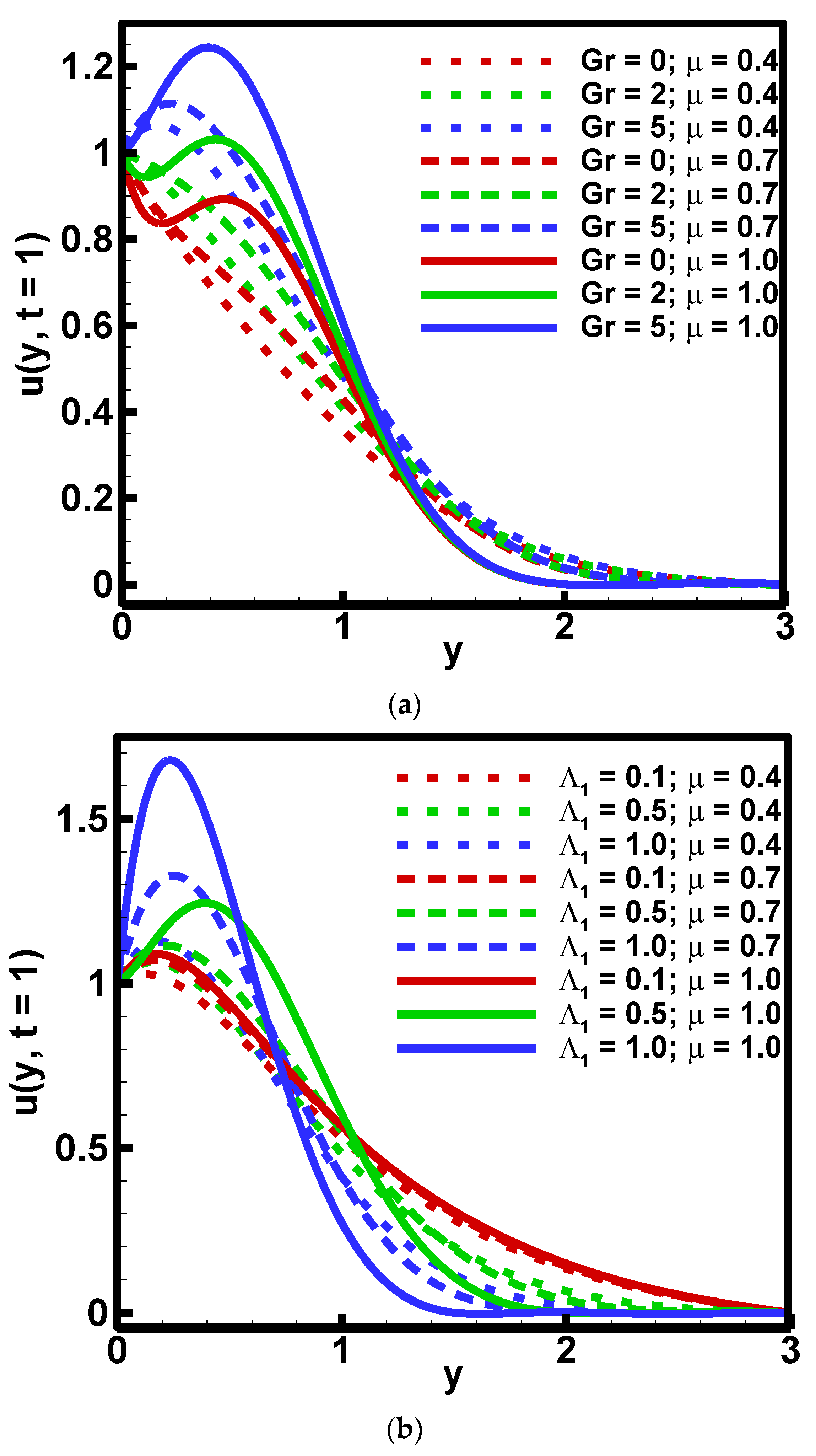
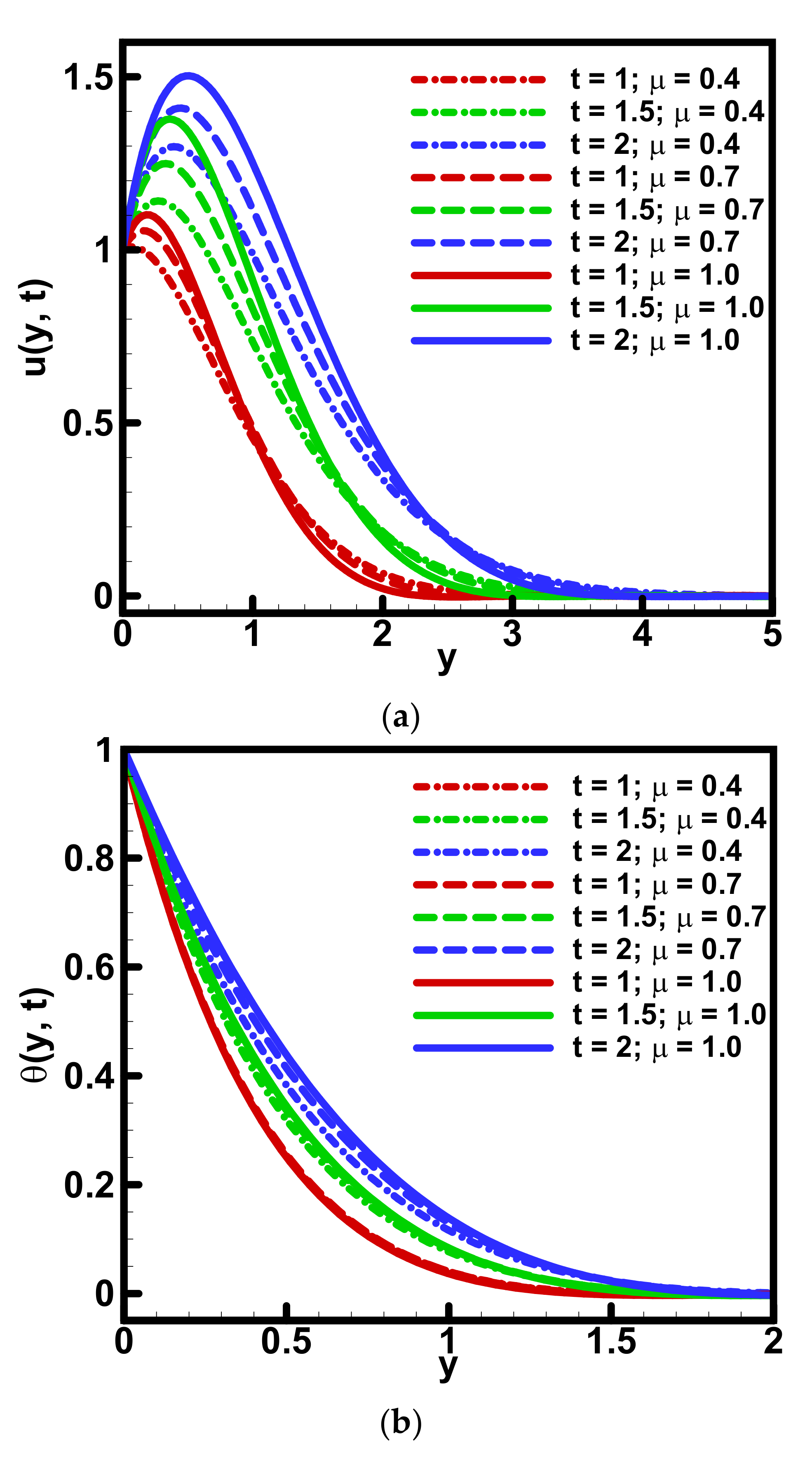
• Velocity increases gradually by the increase in fractional parameters and Grashof number i.e., the relation is direct.
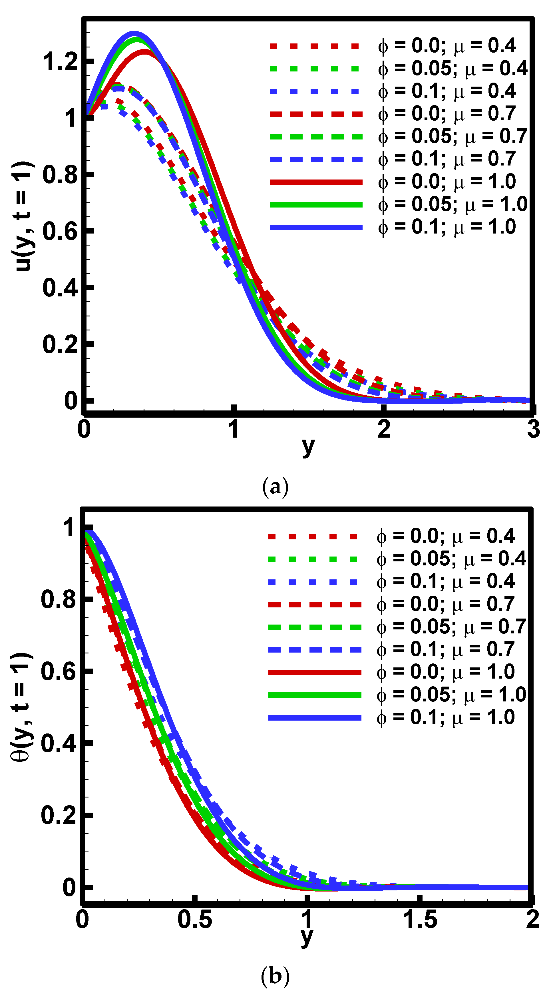
• The enhancement of the volumetric fraction of nanoparticles gives rise to thermal conductivity consequently to the temperature field.
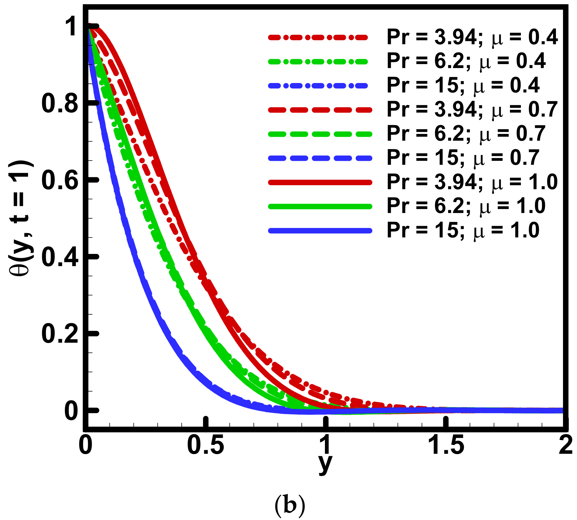
• The velocity profile increases whereas the temperature field is shown to have a descending behavior while increasing the value of the Prandtl number.
• The extended finite difference method produced very accurate and stable solutions against each physical parameter. In other words, the convergence and stability of proposed method have been proved numerically.
• The fractional-order parameter exhibited the dominant influence on the velocity and temperature profiles, and exhibited the increasing behavior against $\alpha .$

References

1. Sheikholeslami, M.; Rashidi, M.M. Effect of space dependent magnetic field on free convection of Fe3O4–water nanofluid. J. Taiwan Inst. Chem. Eng. 2015, 56, 6–15. [Google Scholar] [CrossRef]
2. Sheikholeslami, M.; Vajravelu, K.; Rashidi, M.M. Forced convection heat transfer in a semi annulus under the influence of a variable magnetic field. Int. J. Heat Mass Transf. 2016, 92, 339–348. [Google Scholar] [CrossRef]
3. Sheikholeslami, M. Magnetic field influence on nanofluid thermal radiation in a cavity with tilted elliptic inner cylinder. J. Mol. Liq. 2017, 229, 137–147. [Google Scholar] [CrossRef]
4. Sheikholeslami, M.; Gorji-Bandpy, M.; Ganji, D.D.G.-D.; Rana, P.; Soleimani, S. Magnetohydrodynamic free convection of Al2O3–water nanofluid considering Thermophoresis and Brownian motion effects. Comput. Fluids 2014, 94, 147–160. [Google Scholar] [CrossRef]
5. Sheikholeslami, M.; Hayat, T.; Alsaedi, A. MHD free convection of Al2O3–water nanofluid considering thermal radiation: A numerical study. Int. J. Heat Mass Transf. 2016, 96, 513–524. [Google Scholar] [CrossRef]
6. Sheikholeslami, M. Numerical simulation of magnetic nanofluid natural convection in porous media. Phys. Lett. A 2017, 381, 494–503. [Google Scholar] [CrossRef]
7. Sheikholeslami, M.; Ellahi, R. Three dimensional mesoscopic simulation of magnetic field effect on natural convection of nanofluid. Int. J. Heat Mass Transf. 2015, 89, 799–808. [Google Scholar] [CrossRef]
8. Yu, W.; France, D.M.; Routbort, J.L.; Choi, S.U.S. Review and comparison of nanofluid thermal conductivity and heat transfer enhancements. Heat Transf. Eng. 2008, 29, 432–460. [Google Scholar] [CrossRef]
9. Bejan, A. A Study of Entropy Generation in Fundamental Convective Heat Transfer. J. Heat Transfer. 1979, 101, 718–725. [Google Scholar] [CrossRef]
10. Bejan, A. Second-law analysis in heat transfer and thermal design. In Advances in Heat Transfer; Elsevier: Amsterdam, The Netherlands, 1982; pp. 1–58. [Google Scholar]
11. Bejan, A. The thermodynamic design of heat and mass transfer processes and devices. Int. J. Heat Fluid Flow 1987, 8, 258–276. [Google Scholar] [CrossRef]
12. Bejan, A. Entropy Generation Minimization; CRS Press: Boca Raton, FL, USA, 1996. [Google Scholar]
13. Amiri, I.; Ali, J. Generating highly dark–bright solitons by Gaussian beam propagation in a PANDA ring resonator. J. Comput. Theor. Nanosci. 2014, 11, 1092–1099. [Google Scholar] [CrossRef]
14. Khan, A.; Karim, F.U.; Khan, I.; Alkanhal, T.A.; Ali, F.; Khan, D.; Nisar, K.S. Entropy generation in MHD conjugate flow with wall shear stress over an infinite plate: Exact analysis. Entropy 2019, 21, 359. [Google Scholar] [CrossRef] [Green Version]
15. Awad, M.M. A new definition of Bejan number. Therm. Sci. 2012, 16, 1251–1253. [Google Scholar] [CrossRef] [Green Version]
16. Awad, M.M.; Lage, J.L. Extending the Bejan number to a general form. Therm. Sci. 2013, 17, 631–633. [Google Scholar] [CrossRef]
17. Choi, S.U.; Eastman, J.A. Enhancing Thermal Conductivity of Fluids with Nanoparticles; Argonne National Lab.: Lemont, IL, USA, 1995. [Google Scholar]
18. Friedrich, C. Relaxation and retardation functions of the Maxwell model with fractional derivatives. Rheol. Acta 1991, 30, 151–158. [Google Scholar] [CrossRef]
19. Khan, I.; Shah, N.A.; Mahsud, Y.; Vieru, D. Heat transfer analysis in a Maxwell fluid over an oscillating vertical plate using fractional Caputo-Fabrizio derivatives. Eur. Phys. J. Plus 2017, 132, 194. [Google Scholar] [CrossRef]
20. Imran, M.; Khan, I.; Ahmad, M.; Shah, N.; Nazar, M. Heat and mass transport of differential type fluid with non-integer order time-fractional Caputo derivatives. J. Mol. Liq. 2017, 229, 67–75. [Google Scholar] [CrossRef]
21. Ali, F.; Alam Jan, S.A.; Khan, I.; Gohar, M.; Sheikh, N.A. Solutions with special functions for time fractional free convection flow of Brinkman-type fluid. Eur. Phys. J. Plus 2016, 131, 310. [Google Scholar] [CrossRef]
22. Vieru, D.; Fetecau, C. Time-fractional free convection flow near a vertical plate with Newtonian heating and mass diffusion. Therm. Sci. 2015, 19, 85–98. [Google Scholar] [CrossRef]
23. Khan, I.; Shah, N.A.; Vieru, D. Unsteady flow of generalized Casson fluid with fractional derivative due to an infinite plate. Eur. Phys. J. Plus 2016, 131, 181. [Google Scholar] [CrossRef]
24. Imran, M.A.; Shah, N.A.; Khan, I.; Aleem, M. Applications of non-integer Caputo time fractional derivatives to natural convection flow subject to arbitrary velocity and Newtonian heating. Neural Comput. Appl. 2018, 30, 1589–1599. [Google Scholar] [CrossRef]
25. Asjad, M.I. Fractional mechanism with power law (singular) and exponential (non-singular) kernels and its applications in bio heat transfer model. Int. J. Heat Technol. 2019, 37, 846–852. [Google Scholar] [CrossRef]
26. Aleem, M.; Asjad, M.I.; Shaheen, A.; Khan, I. MHD Influence on different water based nanofluids (TiO2, Al2O3, CuO) in porous medium with chemical reaction and newtonian heating. Chaos Solitons Fractals 2020, 130, 109437. [Google Scholar] [CrossRef]
27. Kaabar, M.K.A.; Martínez, F.; Gómez-Aguilar, J.F.; Ghanbari, B.; Kaplan, M.; Günerhan, H. New approximate analytical solutions for the nonlinear fractional Schrödinger equation with second-order spatio-temporal dispersion via double Laplace transform method. Math. Methods Appl. Sci. 2021, 44, 11138–11156. [Google Scholar] [CrossRef]
28. Eltayeb, H.; Bachar, I.; Kılıçman, A. On Conformable Double Laplace Transform and One Dimensional Fractional Coupled Burgers’ Equation. Symmetry 2019, 11, 417. [Google Scholar] [CrossRef] [Green Version]
29. Asjad, M.I.; Ikram, M.D.; Ali, R.; Baleanu, D. New analytical solutions of heat transfer flow of clay-water base nanoparticles with the application of novel hybrid fractional derivative. Therm. Sci. 2020, 24, 343–350. [Google Scholar] [CrossRef]
30. Khan, I.; Hussanan, A.; Saqib, M.; Shafie, S. Convective heat transfer in drilling nanofluid with Clay nanoparticles: Applications in water cleaning process. BioNanoScience 2019, 9, 453–460. [Google Scholar] [CrossRef]
31. Wang, C.-C. Mathematical Principles of Mechanics and Electromagnetism: Part. A: Analytical and Continuum Mechanics; Springer Science and Business Media: Berlin, Germany, 2013; Volume 16. [Google Scholar]
32. Salah, F.; Aziz, Z.A.; Ching, D.L.C. On accelerated MHD flows of second grade fluid in a porous medium and rotating frame. IAENG International J. Appl. Math. 2013, 43, 106–113. [Google Scholar]
33. Sheikh, N.A.; Ali, F.; Khan, I.; Gohar, M.; Saqib, M. On the applications of nanofluids to enhance the performance of solar collectors: A comparative analysis of Atangana-Baleanu and Caputo-Fabrizio fractional models. Eur. Phys. J. Plus 2017, 132, 540. [Google Scholar] [CrossRef]
34. Zhao, J.; Zheng, L.; Zhang, X.; Liu, F. Unsteady natural convection boundary layer heat transfer of fractional Maxwell viscoelastic fluid over a vertical plate. Int. J. Heat Mass Transf. 2016, 97, 760–766. [Google Scholar] [CrossRef]
35. Khan, A.Q.; Rasheed, A. Numerical simulation of fractional maxwell fluid flow through forchheimer medium. Int. Commun. Heat Mass Transf. 2020, 119, 104872. [Google Scholar] [CrossRef]
36. Cattaneo, C. A form of heat-conduction equations which eliminates the paradox of instantaneous propagation. Comptes Rendus 1958, 247, 431. [Google Scholar]
37. Baleanu, D.; Fernandez, A.; Akgül, A. On a fractional operator combining proportional and classical differintegrals. Mathematics 2020, 8, 360. [Google Scholar] [CrossRef] [Green Version]
38. Abu-Shady, M.; Kaabar, M.K.A. A Generalized Definition of the Fractional Derivative with Applications. Math. Probl. Eng. 2021, 2021, 9444803. [Google Scholar] [CrossRef]
Figure 1. Schematic diagram.
Fractalfract 05 00242 g001
Figure 2. Effect of μ = α = β and (a) Gr when λ 1 α 1 = 0.5, Pr = 15, λ 2 β 2 = 0.7, ϕ = 0.01 (b) λ 1 α 1 when Gr = 5, Pr = 15, λ 2 β = Λ2 = 0.7, ϕ = 0.01 on the velocity profiles.
Fractalfract 05 00242 g002
Figure 5. Behavior of (a) velocity and (b) temperature profiles as varying μ = α = β and t when λ 1 α 1= 0.5, ϕ = 0.01, λ 2 β 2 = 0.7, Gr = 5, Pr = 15.
Fractalfract 05 00242 g005