A Spatially Distributed Network for Tracking the Pulsation Signal of Flow Field Based on CFD Simulation: Method and a Case Study

Abstract

The pulsating characteristics in turbulent flow are very important physical quantities. There are many studies focused on the temporal characteristics of pulsation. However, the spatial distribution of temporal states with pulsations rarely receives attention. Therefore, the pulsation tracking network (PTN) method is proposed to track the pulsating characteristics of turbulence. Based on the computational fluid dynamics (CFD) simulation result, the PTN is arranged in a specific region of the flow domain. The fast Fourier Transform (FFT) method is used for time-frequency conversion. As shown in the example of trailing-edge vortex-shedding flow over NACA0009 hydrofoil, important pulsation quantities, including the total pulsation intensity, dominant frequencies, amplitude of frequencies, and the phase and phase difference, can be obtained with a high spatial resolution. The source, reason and attenuation of the vortex-shedding frequency f_vs and the 2 f_vs frequency caused by vortex-interaction are well indicated. The dominant regions of f_vs and 2 f_vs are shown and analysed. The propagation and attenuation of vortex-shedding induced pulsation are understood in detail. Based on the comparison against traditional analysis, PTN is found to function as a good supplement for the CFD post-processing by tracking unknown temporal and spatial characteristics. These findings represent a potential breakthrough in terms of solving actual pulsation-excited flow problems.

1. Introduction

Karman vortex street is an important phenomenon in viscous incompressible fluid dynamics. The study of Karman vortex street is usually based on the case of flow around a cylinder or a foil [1,2]. In recent years, the research methods of temporal and spectral characteristics of flow fields were gradually applied to unsteady flow fields [3,4]. The modal decomposition of flow fields can be divided into two categories: one is based on data-driven approaches (POD, SPOD and DMD). The second is based on operator-driven approaches (Koopman analysis, global linear analysis, stability analysis and resolvent analysis).

The former is based on flow field data, such as CFD calculation results and experimental measurements; The latter is based on the linearized N-S equation. However, its most obvious advantage is that it has no requirements for input, that is, this data can be linear or nonlinear, and the results can be numerical or experimental. This approach does not necessarily even involve the calculation results of a flow field. The essence of model reduction is to project the system into a smaller vector space that can describe the parameters.

The essence of POD is to find low dimensional subspaces (i.e., flow modes or coherent structures), and it expresses the high-dimensional and complex unsteady flow field as the superposition of these subspaces on the low dimensional coordinate system. The flow field evolution in the low dimensional space was previously described, and the dominant vortex structure in the unsteady flow field was identified [5]. Lumley [6,7] identified the coherent structure in a turbulent flow field by means of the orthogonal decomposition of a spatial velocity correlation function [8], which was called direct-POD. With the rapid development of experimental and numerical simulations, the original data that need to be de-composed is increasingly large and complex, which leads to the large dimensions of the flow field information matrix. The direct-POD method cannot solve its eigenvalues and eigenvectors. Sirovich [9] improved the direct-POD method and put forward the concept of space-time conversion. He used a time cross-correlation matrix instead of a space cross-correlation matrix and successfully solved the problem of too many space points. This method is called snapshot-POD. The dominant coherent structure distribution can be identified by sorting the proportion of each mode of energy [10,11]. The main characteristic of this method is the relationship between the reduced data and the original data, including the numerical relationship among the mean value, eigenvector and principal component [12]. However, the frequency analysis of the pulsating signal is slightly insufficient in the POD method.

SPOD (spectral proper orthogonal decomposition) expands the POD and was published by Towne [4] in 2018. POD decomposes the data into the eigenmode, eigenvalue (energy), etc. However, this evolution coefficient cannot be expressed as a specific function of time. Furthermore, the time series can be represented by a regular time function via the Fourier transform method. SPOD realizes the time-space conversion by converting the time domain to the frequency. SPOD expands the time orthogonality and retains all the characteristics of POD.

DMD involves the extraction of dynamic information from unsteady experimental measurement or numerical simulation flow fields, and was proposed by Schmid [13,14]. In essence, the flow evolution is regarded as a linear dynamic process. Through the characteristic analysis of the flow field snapshot of the whole process, the low-order modes and their corresponding eigenvalues (or Ritz values) are obtained. The most important feature of this method is that the decomposed mode has a single frequency and growth rate [15].Therefore, it has great advantages in the analysis of dynamic linear and periodic flow, but needs to occupy a lot of data storage space. Kunihiko et al. [16] described some of the main techniques used to complete these modal decompositions and analyses. These techniques have been booming in recent decades. Some mature techniques are briefly introduced, and the framework of these methods is clearly established by using familiar linear algebra. Pan et al. [17] applied DMD to study the wake velocity field of NACA0015 airfoil measured by TR-PIV. The spatial motion of vortex pairs usually shows the coupling of long wave and short-wave modes.

The parameters of the periodic signal mainly include the frequency, phase and amplitude [18]. The amplitude is directly obtained by analysing the sampled values in the time series (time domain analysis), but many problems require information about the pulsation frequency. In the frequency domain analysis, the distribution of signal strength relative to frequency is studied, which is expressed by the spectrum. The spectrum value is complex, the spectrum has real and imaginary parts, and each frequency has a phase angle [19]. The amplitude spectrum is the description of signal contour and shape. The phase spectrum is a description of the signal position. The amplitude spectrum of signals with the same shape is the same at different positions, but the phase spectrum is different [20,21]. In other words, the frequency reflects the frequency of the pulse. The amplitude indicates the intensity of the pressure pulsation. The phase represents the state of the signal at a specific time.

In this study, we introduce a pulsation tracking network (PTN) method for the tracking of turbulent pulsation characteristics. The frequency decomposition of the flow field pulsation signal is studied. This method allows for a better understanding of important parameters, including the amplitude, peak-to-peak value, dominant frequency, phase and phase difference, pulsation attenuation and pulsation propagation. A simple case of hydrofoil trailing-edge vortex-shedding flow is used as an example to show the main functions of PTN. Traditional analyses are also conducted for pressure pulsation to show the advantages of PTN. Innovative results will be shown in the following sections. The results will demonstrate that PTN could be a breakthrough and an effective supplement to CFD simulation, especially in post-processing.

2. Temporal Spatial States of Pressure Pulsation

Based on FFT, a periodic signal can be represented as the addition of different sinusoidal (or cosine) signals, and these sinusoidal (or cosine) signals are orthogonal. Through the integral Fourier Transform formula, the frequency and amplitude of these sinusoidal (or cosine) signals can be solved accurately. The frequency domain diagram can be obtained as follows:

$$\begin{array}{l}f(t)=\frac{1}{2\pi }{\displaystyle {\int }_{-\infty }^{+\infty }F}\left(\omega \right)\cdot e^{i\omega t}d\omega \\ F\left(\omega \right)={\displaystyle {\int }_{-\infty }^{+\infty }f}(t)e^{-i\omega t}dt\end{array}$$

(1)

where ω = n·Δω (n = 1, 2, 3 …), and Δω can be considered as the frequency interval of the periodic function of adjacent frequencies.

Furthermore, the pulsation of pressure ΔP can be expressed as:

$$\Delta P=P_{\max }-P_{\min }$$

(2)

where P_max is the maximum value defined in the pressure pulsation, and P_min is the minimum value. In order to avoid the error caused by signal interference, a certain confidence interval (for example, 97%) is considered when calculating the peak-to-peak value according to the IEC regulations [22].

For a certain frequency (the main frequency is shown here), the phase of a certain point is selected as the initial phase φ₀, and the phase at point k is expressed as φ_k. The FFT characteristic frequency phase difference Δφ_k can be calculated as follows:

$$\Delta {\phi }_k=\left|{\phi }_k-{\phi }_0-2m\pi \right|$$

(3)

where $\{\begin{array}{c}{\phi }_0>0\\ {\phi }_k\le {\phi }_0-\pi \end{array},n=-1$; $\{\begin{array}{c}{\phi }_0\le 0\\ {\phi }_k\le {\phi }_0+\pi \end{array}\mathrm{or}\{\begin{array}{c}{\phi }_0>0\\ {\phi }_k>{\phi }_0-\pi \end{array},n=0$; $\{\begin{array}{c}{\phi }_0\le 0\\ {\phi }_k>{\phi }_0+\pi \end{array},n=1$. The value of the $\Delta {\phi }_k$ range is $0~\pi$. The values of the ${\phi }_k$ and ${\phi }_0$ ranges are $-\pi ~\pi$.

3. Pulsation Tracking Network (PTN) Method

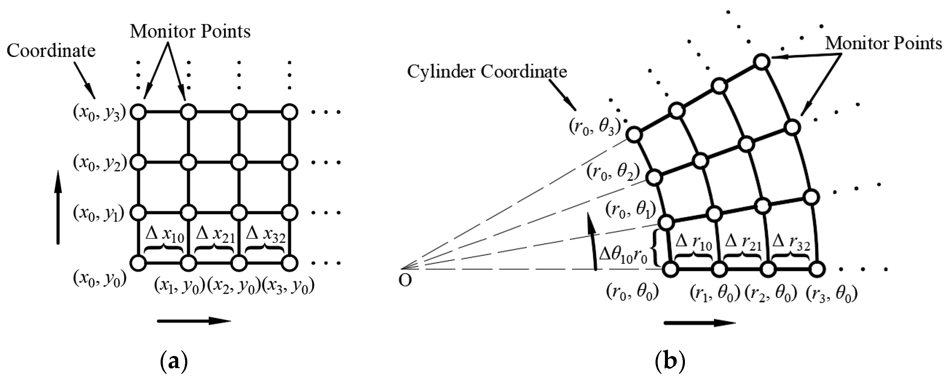
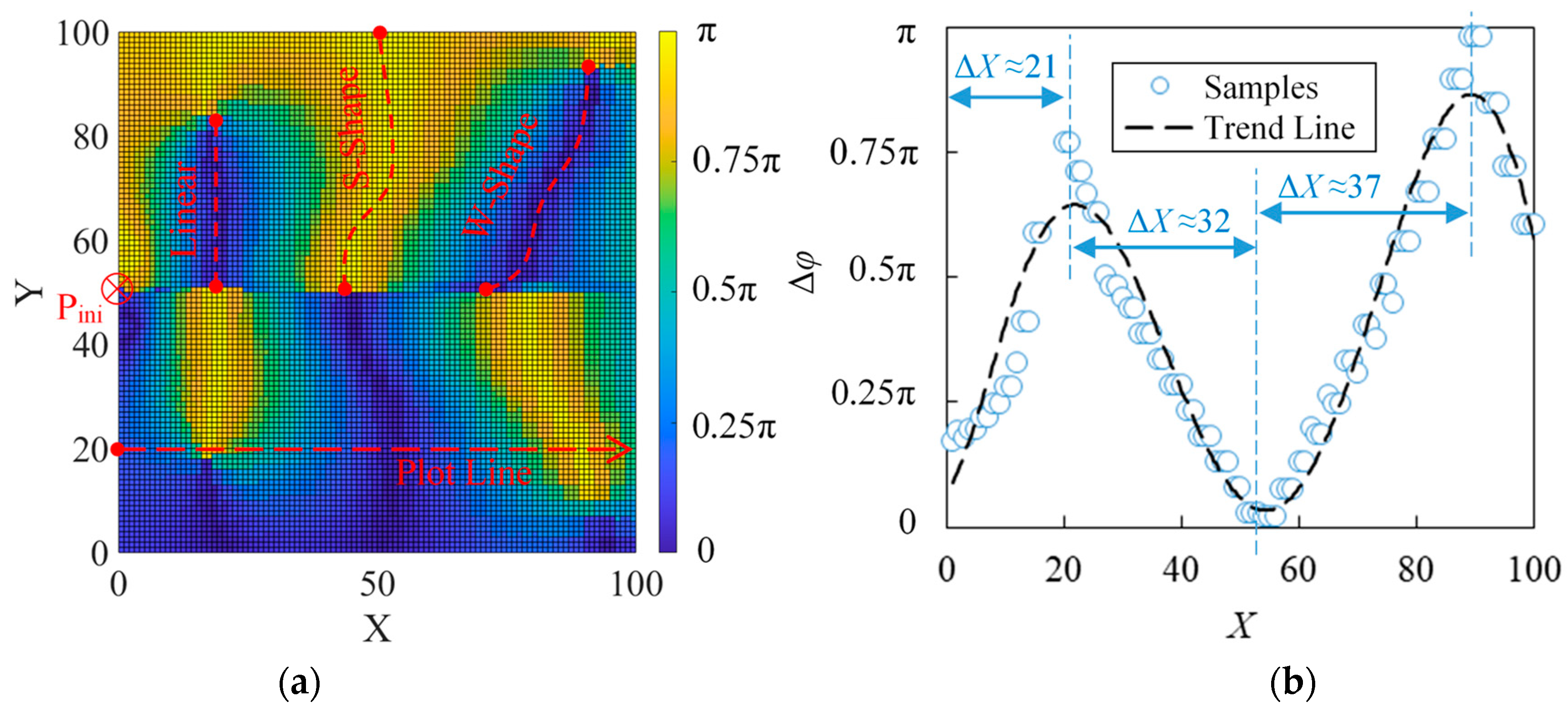
3.1. Estimated Distance of Adjacent Monitoring Points

A large number of ordered monitoring points should be well distributed in the flow field to prepare for PTN. Thus, there is a necessary parameter, the estimated distance of adjacent monitoring points, denoted as D_E, which can be expressed as follows:

$$D_E=\frac{c_s{U}_{ref}}{2\pi f_{max}}$$

(4)

where U_ref is a reference flow velocity, m/s; f_max is the maximum main frequency in the monitoring area, Hz; c_s is the safety factor, which controls the density of monitoring points and is used to refine the length of D_E for a better resolution. According to experience, c_s ranges from 0.1 to 1.0. D_E is essentially a choice of the density of PTN monitoring points, which will directly affect the resolution of the simulated results. This will be discussed in Section 6.1.

3.2. Layout Scheme of Monitoring Points

A large number of monitoring points should be arranged in the simulation area. Different from grid nodes, these monitoring points are used to monitor and record pressure pulsation. The layout mode of monitoring points can be adjusted according to the topology of the monitoring area. In the example of a two-dimensional (2D) case, as shown in Figure 1a, the monitoring points can be arranged evenly in the Cartesian coordinate system. For the rotor and stator of rotating machinery, the Cylinder coordinate system could be improved by using the monitoring point arrangement mode shown in Figure 1b.

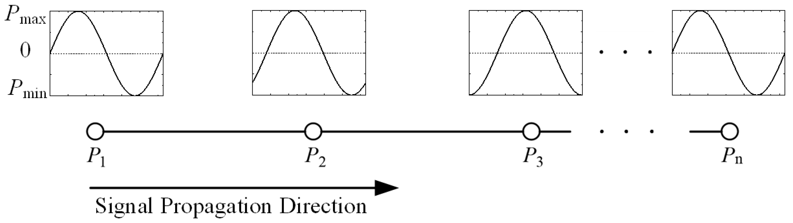
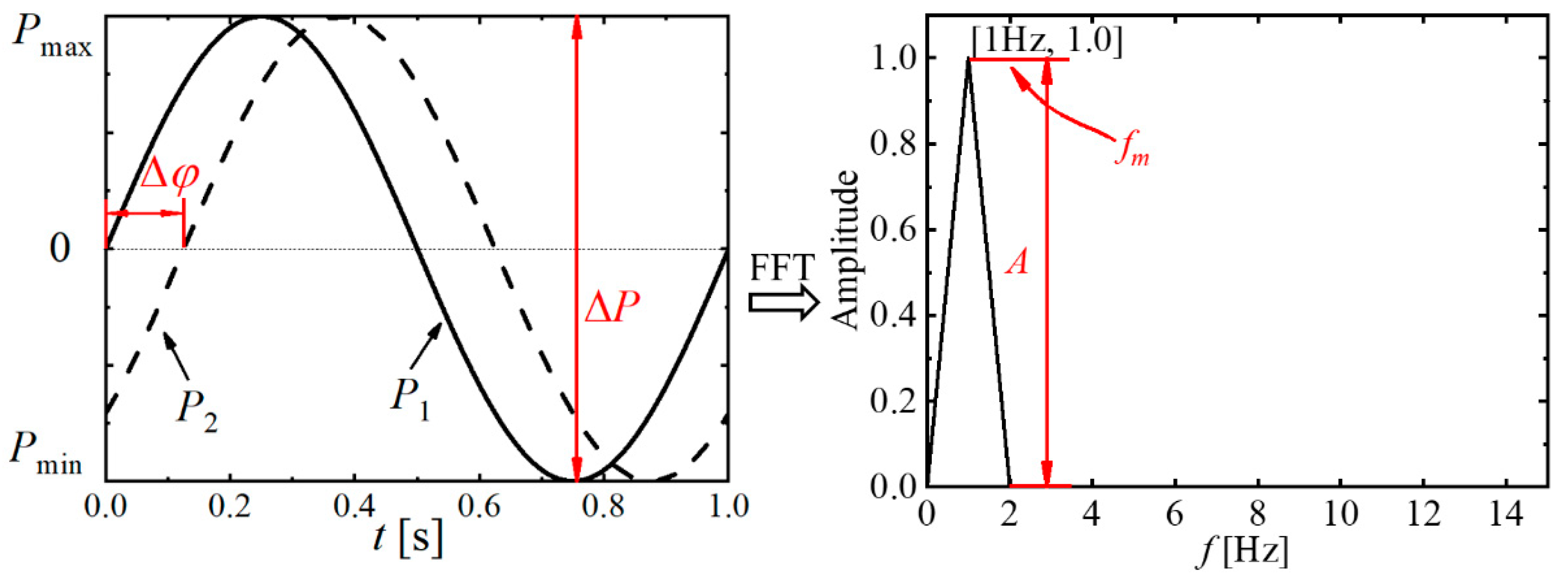
3.3. The Process of Signal Propagation

A pulsating signal can be propagated in a certain direction in space, and the ideal propagation process is shown in Figure 2. The signal at P₁ propagates in a certain direction, and it passes one period just after transmitting to P_n. Each point has phase difference behind the previous point, as shown in Figure 3. However, the amplitude (A) and main frequency (f_m) remain unchanged during propagation.

Because of the signal intensity attenuation, the propagation of Δφ and ΔP from P₁ to P₂ and from P₂ to P₃ was not equal in the actual situation. If another signal comprising other points was propagated here, it would have made the signal more disordered. It was difficult to trace back to the signal source. PTN methods can also provide solutions for signal traceability.

4. Testing Case Details

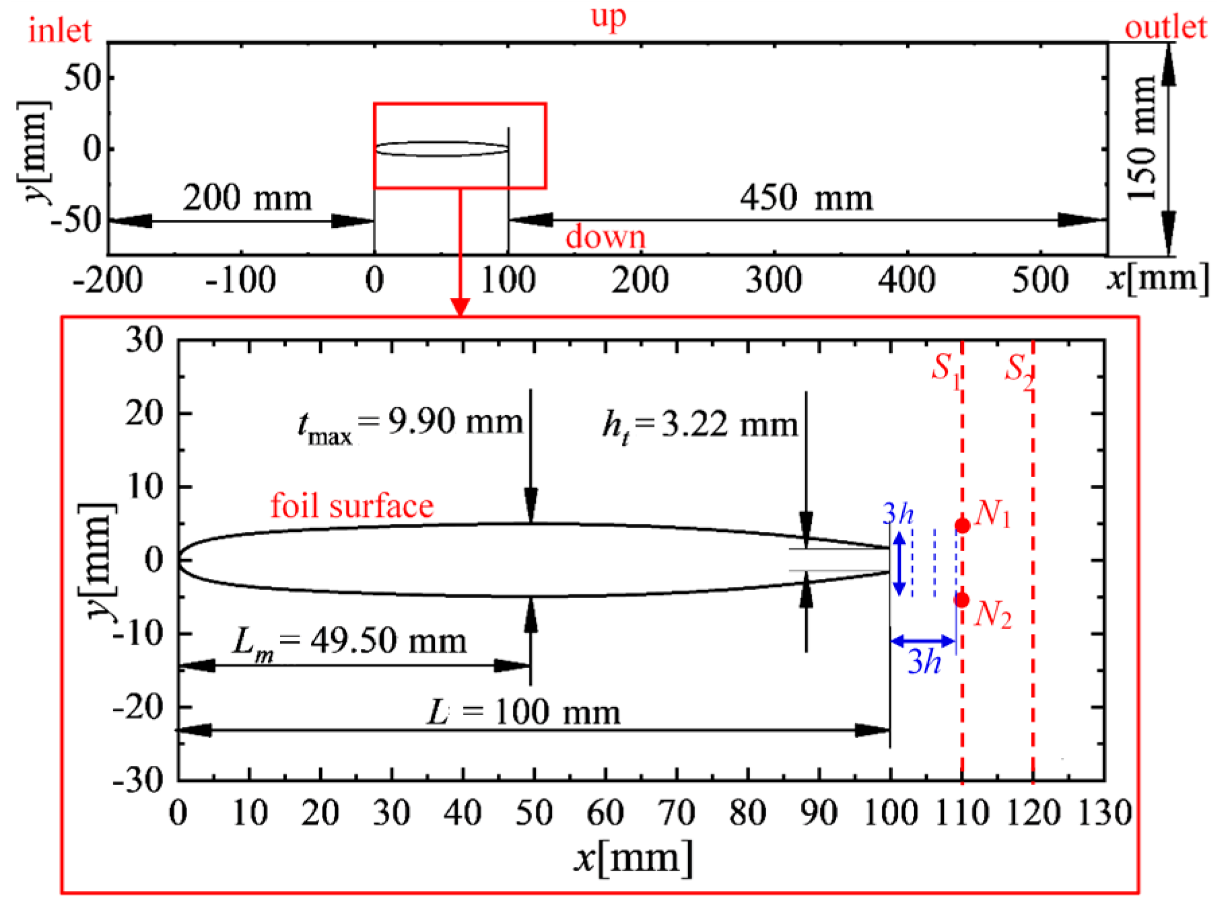
4.1. Case Description

As a typical fluid dynamic’s phenomenon, trailing-edge vortex shedding generates very regular pulsations. Even though its time-domain and frequency-domain are widely studied by researchers, the relevant pulsation intensity, the cover range of frequencies and the spatial distributions of temporal states are not fully understood. Therefore, this study took the trailing-edge vortex-shedding case of symmetrical NACA0009 foil as the research object [23,24]. A comparative case testing process was conducted in this study by comparing traditional analysis and PTN analysis. For simplification in this comparative testing process, the 2D flow domain is discussed as shown in Figure 4. The chord length L was shortened from 110 to 100 mm. The trailing-edge thickness of the hydrofoil was h_t = 3.22 mm. The maximum thickness of the hydrofoil was t_max = 9.90 mm. The distance from the maximum thickness to the leading-edge was L_m = 49.50 mm. The incidence angle was 0 degrees. The incoming flow velocity U_ref was 20 m/s and the Reynolds number $R{e}_h=U_{ref}{h}_t/\upsilon$ was approximately 64.4 × 10³. The Strouhal number $S{t}_h=h_{t}f/U_{ref}$ was approximately 0.19.

The ANSYS CFX computational code was utilized to simulate the flow fields. The Reynolds-averaged Navier-Stokes (RANS) equations were used in this case, also taking into account the total energy equation. The SST k-ω turbulence model [25,26,27] was used to close the RANS equations. Furthermore, the transport equations of the turbulent kinetic energy k and specific dissipation rate ω can be expressed as:

$$\frac{\partial (\rho k)}{\partial t}+\frac{\partial \left(\rho u_{i}k\right)}{\partial x_i}=P-\frac{\rho k^{3/2}}{l_{k-\omega }}+\frac{\partial }{\partial x_i}\left[\left(\mu +{\sigma }_k{\mu }_t\right)\frac{\partial k}{\partial x_i}\right]$$

(5)

$$\begin{array}{l}\frac{\partial (\rho \omega )}{\partial t}+\frac{\partial \left(\rho u_i\omega \right)}{\partial x_i}=C_{\omega }P-\beta \rho {\omega }^2+\frac{\partial }{\partial x_i}\left[\left({\mu }_l+{\sigma }_{\omega }{\mu }_t\right)\frac{\partial \omega }{\partial x_i}\right]\\ +2\left(1-F_1\right)\frac{\rho {\sigma }_{\omega 2}}{\omega }\frac{\partial k}{\partial x_i}\frac{\partial \omega }{\partial x_i}\end{array}$$

(6)

where ρ is the fluid density, P is the turbulence generation term, μ is the dynamic viscosity, μ_t is the eddy viscosity coefficient, σ is the model constant, C_ω is the coefficient of turbulent dissipation term, F₁ is the blending equation, and l_k-ω is the scale of turbulence.

The grid scheme used in the 2D computational domain had 81,026 nodes, and the grid elements were quadrilateral structured 2D elements. The range of y⁺ on the wall was controlled within the range of 2~13 for the application of wall functions in the near wall region. The boundary conditions were set as shown in

Table 1. Boundary conditions.

No.	Position	Type	Description
1	Inlet	Velocity inlet boundary	vin = 20 m/s
2	Outlet	Pressure outlet boundary	pout = 1 atm
3	Foil Surface	Wall	No slip wall
4	Up and Down Walls	Wall	No slip wall
5	Two Sides	Symmetry	Simplified for 2D

. Transient simulation was carried out based on the steady results. The time-step of transient computation was set to 1.0 × 10⁻⁵ s. As for the discretization schemes, the central difference scheme was adopted for the diffusion term, the second-order upwind scheme was used for the convective term, while the second-order backward Euler scheme was employed for the transient term. A fully implicit coupling algorithm was employed for transient computation, while the convergence residual standard was set to 1.0 × 10⁻⁵.

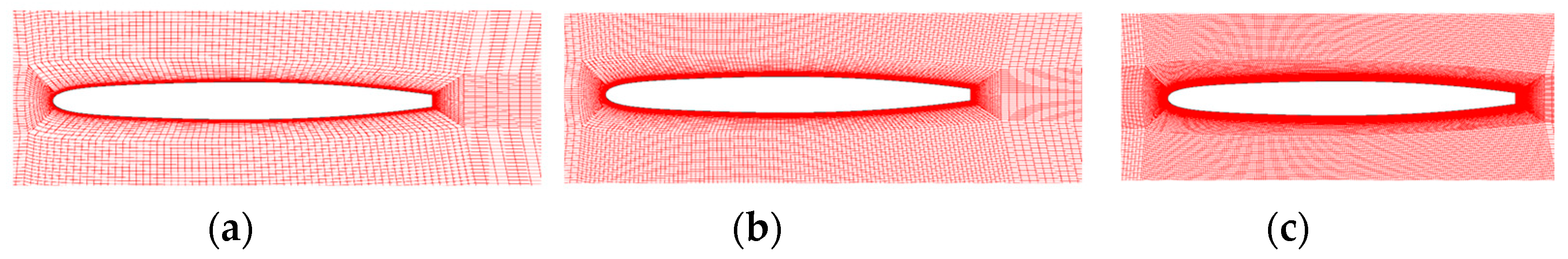
4.2. Grid Convergence Check

To obtain a better reliability for the CFD simulation, the grid convergence index (GCI) was studied based on Richardson’s extrapolation method [28]. G₁, G₂ and G₃ which are three grid schemes, were determined proportionally, as shown in Figure 5. The grid refinement factors were as follows: r₂₁ = 1.32 and r₃₂ = 1.31. The mesh node numbers of the three grids were G₁ = 112,844 (x: 303 nodes; y: 175 nodes), G₂ - 197,240 (x: 401 nodes; y: 229 nodes) and G₃ = 338,200 (x: 531 nodes; y: 301 nodes). As indicated in Figure 4, two points (N₁ (x = 110 m, y = 5 mm) and N₂ (x = 110 mm, y = −5 mm)) and two lines (S₁ (x = 110 mm), S₂ (x = 120 mm)), located near the trailing edge of the hydrofoil, were selected for GCI verification. The parameters P_N1 (average value of pressure fluctuation at N₁), P_N2 (average value of pressure fluctuation at N2), P_S1 (average value of pressure at S₁), P_S2 (average value of pressure at S₂), v_N1 (average value of velocity at N₁) and v_N2 (average value of velocity at N2) were used as indexes, and these are listed in

Table 2. Evaluation results of discretization error in GCI check.

	PN1 (kPa)	PN2 (kPa)	PS1 (kPa)	PS2 (kPa)	vN1 (m/s)	vN2 (m/s)
ϕ1	124.71	124.65	102.58	103.85	19.256	19.248
ϕ2	125.90	125.87	102.87	103.80	19.252	19.237
ϕ3	126.34	126.29	103.28	103.89	19.282	19.280
p	3.9499	4.1191	1.1813	2.3226	7.2465	4.9176
${\varphi }_{\mathrm{ext}}^{21}$	124.08	124.06	101.81	103.91	19.256	19.2520
$e_a^{21}$	0.96%	0.98%	0.28%	0.05%	0.02%	0.06%
$e_{\mathrm{ext}}^{21}$	0.51%	0.48%	0.76%	0.05%	0.003%	0.02%
${\mathrm{GCI}}_{\mathrm{fine}}^{21}$	0.63%	0.60%	0.94%	0.07%	0.004%	0.03%
${\varphi }_{\mathrm{ext}}^{32}$	125.69	125.67	101.81	103.70	19.247	19.222
$e_a^{32}$	0.35%	0.34%	0.40%	0.09%	0.15%	0.22%
$e_{\mathrm{ext}}^{32}$	0.17%	0.16%	1.04%	0.10%	0.02%	0.07%
${\mathrm{GCI}}_{\mathrm{fine}}^{32}$	0.22%	0.20%	1.29%	0.12%	0.03%	0.09%

. The apparent-order, represented as p, ranged from 1.1813 to 7.2465, and the extrapolation values ${\varphi }_{\mathrm{ext}}^{21}$ and ${\varphi }_{\mathrm{ext}}^{32}$ were acquired. The approximate relative error ${\mathrm{e}}_{\mathrm{a}}^{21}$ was in the range of 0.02 to 0.98%, and ${\mathrm{e}}_{\mathrm{a}}^{32}$ was in the range of 0.09 to 0.40%. The discretization uncertainty ${\mathrm{e}}_{\mathrm{ext}}^{21}$ was in the range of 0.003 to 0.76%, and ${\mathrm{e}}_{\mathrm{ext}}^{32}$ was in the range of 0.02 to 1.04%. The convergence index of G₁ ${\mathrm{GCI}}_{\mathrm{fine}}^{21}$ was in the range of 0.004 to 0.94%, and ${\mathrm{GCI}}_{\mathrm{fine}}^{32}$ was in the range of 0.03 to 1.29%. Hence, G₂ was selected as a compromise between accuracy and computational cost with a total of 197,240 nodes.

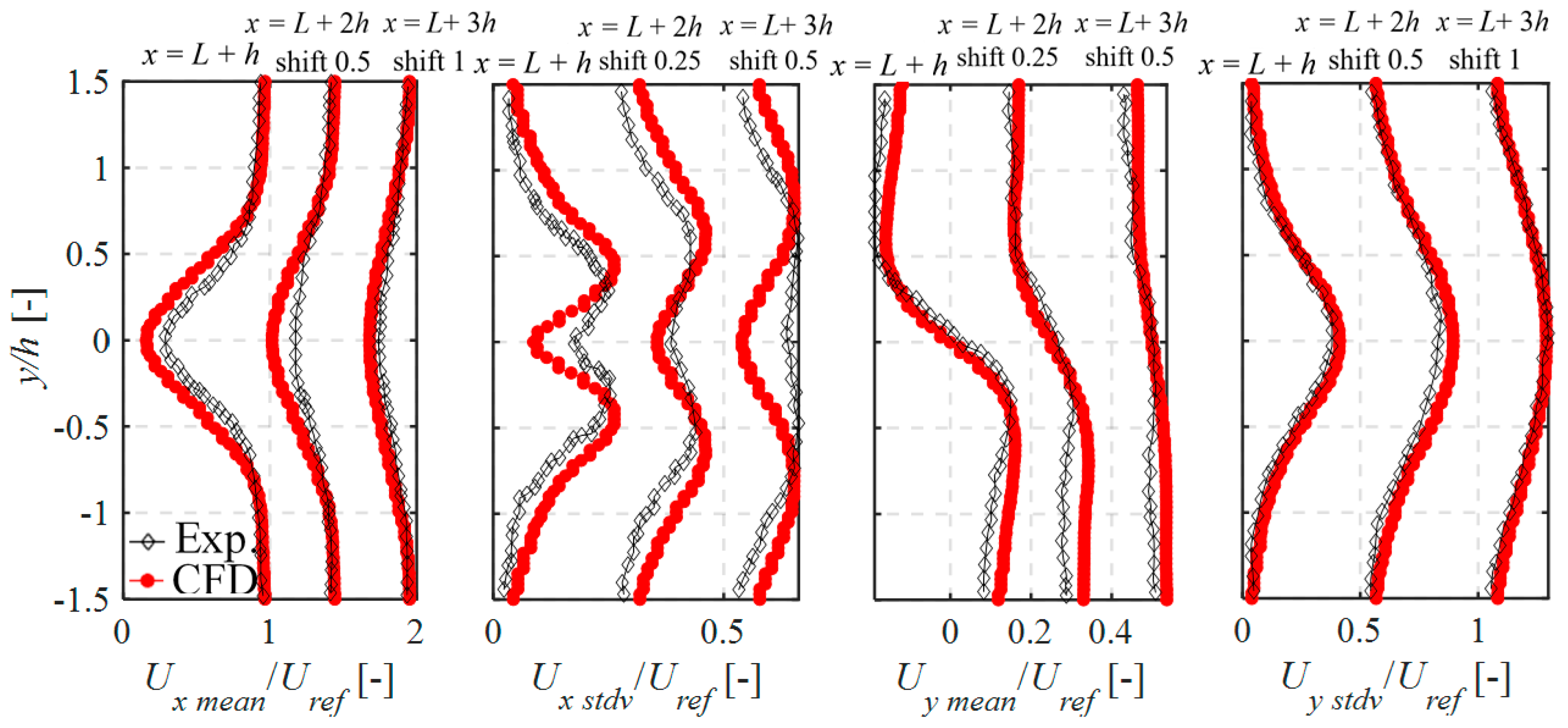
4.3. Experimental-Computational Validation

In this study, the velocity of the inlet flow was 20 m/s. Because of the vortex-shedding, strong pressure and velocity changes downstream of the trailing edge of the hydrofoil were expected. Based on the experimental data [24], the numerical trailing-edge flow field could be validated by considering the decomposition of the velocity with the time-averaged and pulsating components. The two components can be expressed as follows:

$$U_{mean}=\frac{1}{N}{\displaystyle \sum _{i=1}^n{U}_i}$$

(7)

$$U_{stdv}=\sqrt{\frac{1}{N}{\displaystyle \sum _{i=1}^N{\left(U_i-U_{mean}\right)}^2}}$$

(8)

where U_i is the transient velocity; U_mean is the time-averaged velocity; U_stdv is the root mean square of the velocity component; and N presents the number. The experimental-computational validation is shown in Figure 6 by plotting the U_mean/U_ref and U_stdv/U_ref curves on three reference lines. The reference velocity U_ref was equal to the upstream velocity of 20 m/s. As indicated in Figure 4, the three lines were distributed downstream from the trailing-edge with the distance of h = h_t = 3.22 mm between every two lines. The y-direction lengths of the three lines were also 3h. For the pulsating velocity in the x-direction, U_{x stdv}, the maximum difference was 0.09 between the experimental results and the computational results on the first line, and the maximum difference was 0.10 between the experimental results and the computational results on the third line. It can be found that the time-averaged velocity in the x-direction U_{x mean}, the time-averaged velocity in the y-direction U_{y mean}, and the pulsating velocity in the y-direction U_{y stdv}, were in good agreement with the experimental results. Some researchers [29,30] used the same method to calculate the shedding frequency of the Karman vortex street at the trailing edge of the hydrofoil.

5. Traditional CFD Post-Processing

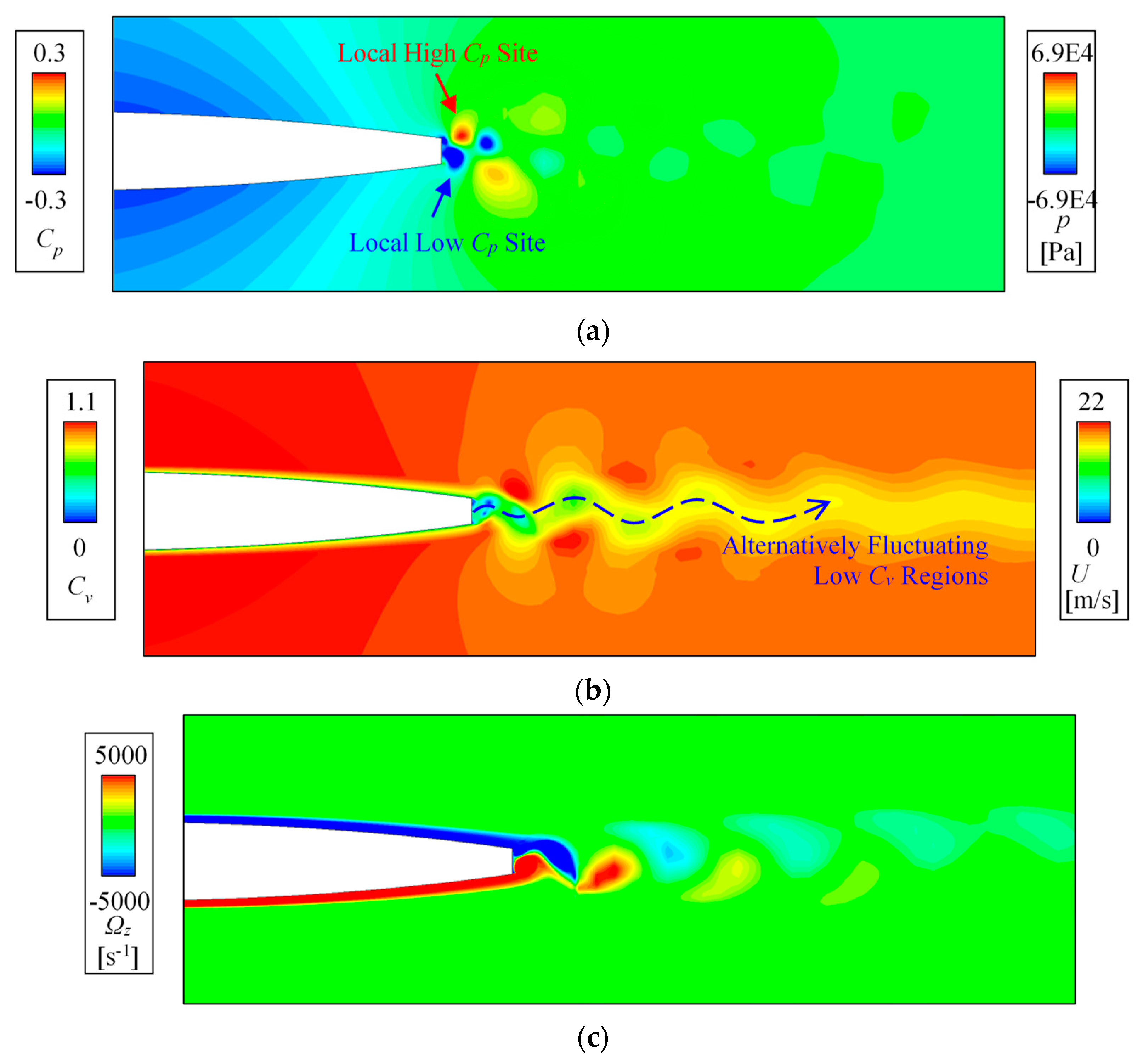
5.1. Flow Patterns of Trailing-Edge Vortex Shedding

Based on the CFD simulation result, the flow patterns of trailing-edge vortex shedding can be analysed as shown in Figure 7. Both the pressure p and the dimensionless pressure coefficient C_p are tagged as shown in Figure 7a. The dimensionless pressure coefficient C_p can be expressed as:

$$C_p=\frac{2\left(p-p_{ref}\right)}{\rho U_{ref}^2}$$

(9)

where ρ is the density, and p_ref is the reference pressure at the inlet boundary. Local high and low C_p sites could be alternately found in the vortex-shedding region. Figure 7b shows the contour of velocity. Both the velocity U and normalized velocity coefficient C_v are tagged. The velocity coefficient C_v can be calculated by:

$$C_v=U/U_{ref}$$

(10)

Alternatively, local low C_v regions could be found fluctuating along the x direction. Both the C_p and C_v patterns indicated the alternative pattern, which was the typical pattern of the trailing-edge vortex-shedding flow. Therefore, it was necessary to plot the vorticity Ω_z perpendicular to x-y plane in Figure 7c. This clearly shows the shedding vortexes downstream of the trailing edge with the decreasing intensity of Ω_z along the x direction.

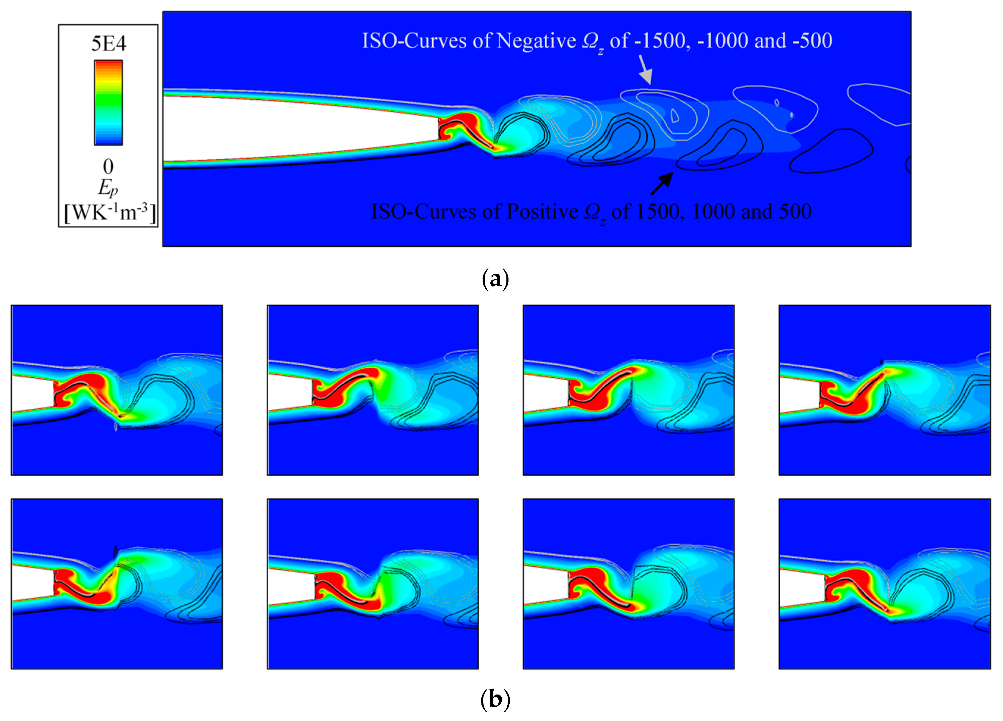
5.2. Interactions among Vortexes

The decreasing intensity of Ω_z indicates the interactions among the shedding vortexes. Figure 8a shows the pattern of entropy production and the ISO-Ω_z curves at a specific time step. The entropy production E_p can approximately show the energy dissipation due to flow-flow interaction [31]. It can be expressed as:

$$E_p=C_e\rho k\epsilon /T$$

(11)

where k is the kinetic energy of the turbulence, ε is the eddy dissipation of the turbulence, and T is the temperature. Negative and positive ISO-Ω_z curves represent the instantaneous positions of the vortexes. The high E_p sites appeared mainly in the interaction regions between a positive Ω_z vortex and a negative Ω_z vortex. Figure 8b shows the pattern of E_p and Ω_z of eight continual time steps, with a time difference of 0.0001 s between each two steps. It was found that, in general, the periodic shedding of vortexes would periodically cause high-flow energy dissipation.

5.3. Pressure Pulsation on Typical Sites

Pressure pulsation is one of the most important transient phenomena in vortex-shedding flow cases. Therefore, in this study, it was necessary to analyse the pressure pulsation with both time-domain and frequency-domain plots. In traditional pressure pulsation analyses, discrete monitoring points can be distributed in the concerned region. As shown in Figure 9a, a total of nine points were set in the vortex-shedding region, and were denoted as T₁~T₃, M₁~M₃ and D₁~D₃. The distance between two adjacent points was 5 mm and the distance between M₁ and the trailing-edge was also 5 mm.

Figure 10 includes the time-domain plot and frequency-domain plot of the pressure pulsation on the nine points. The time-domain waveforms were strongly periodic within 0.006 s. The pressure values on T₁~T₃ and D₁~D₃ were similar, which shows the symmetry of vortex-shedding flow. The pressure values on M₁~M₃ were around 0 Pa because M₁~M₃ were approximately located on the y = 0 line. On the frequency-domain plot of the root mean square (RMS) value of pressure, two special frequencies were found. The 1152 Hz frequency denoted by f_vs was the main frequency of points T₁~T₃ and D₁~D₃. The 2304 Hz frequency denoted by 2 f_vs (1152 Hz × 2) was the main frequency of points M₁~M₃. It was clear that f_vs was the vortex-shedding frequency. T₁~T₃ and D₁~D₃ were dominated by this frequency because they were symmetrically distributed on the two sides of y = 0 line. M₁~M₃ were dominated by 2 f_vs because they were located in the interaction region between two vortex rows. However, the influence range and variation law of f_vs and 2 f_vs could not be fully understood based on the traditional method of analysis. Phase and phase differences could be also found on the time-domain plot but were not very clear for the purpose of comparison and analysis.

6. PTN Tracking Results

6.1. Setup of PTN

In Section 3.1, the parameter c_s was defined to adjust the density of the layout of the monitoring points. The graphic resolution of different c_s values is discussed in this part. The specific selected parameters are analysed in detail in the following sections, as shown in Figure 11, which includes a comparison of c_s = 0.145, 0.290, 0.435, 0.580, 0.725 and 1.000. It can be seen that the graphic resolution directly affected the display result. Low resolution led to the over-enlargement of high and low areas, and the capture of spatial distribution was not sufficiently smooth. In this study, the result with the smallest c_s was used for analysis in order to obtain high-resolution simulation results.

As shown in Figure 9b, a total of 10,201 monitoring points were distributed in an evenly-spaced pattern downstream of the trailing edge of the hydrofoil. These points were coded by X000~X100 along the x-direction and Y000~Y100 along the y-direction. The parameters in Equation (2) could thus be determined as D_E = 0.2 mm and c_s = 0.145. Therefore, these 10,201 points covered a 20 mm × 20 mm region. The relative point position X and Y are used in the following sections for a better comparative analysis. In the following PTN analyses, the total sampling time is 0.1 s.

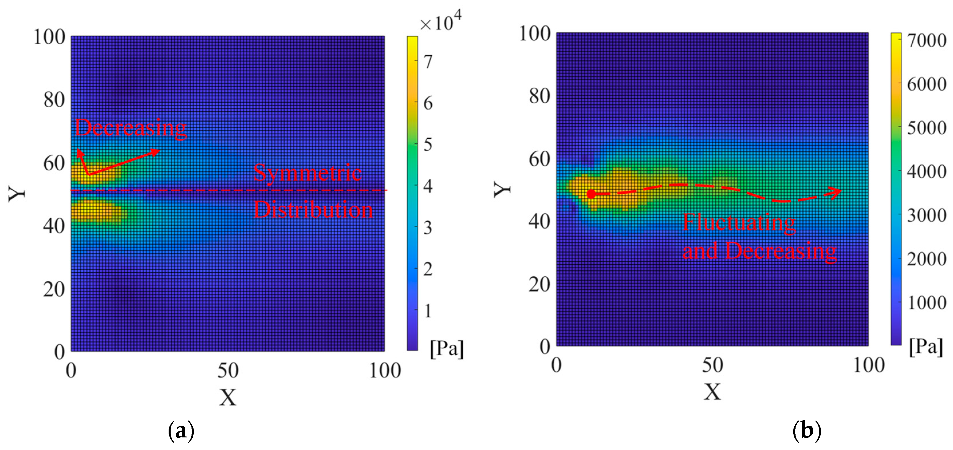
6.2. Amplitude

As found in Figure 10, the vortex-shedding frequencies f_vs and 2 f_vs were the dominant frequencies in this case. Thus, the RMS amplitude values of f_vs and 2 f_vs were analysed based on the PTN, as shown in Figure 12. As shown in Figure 12a, the RMS amplitude of f_vs was symmetrically distributed (along Y = 50) downstream of the trailing edge of the hydrofoil because the vortex was alternately shedding in two rows. The strongest f_vs regions were located at approximately X = 6, Y = 54 and X = 6, Y = 46. The highest amplitude of f_vs was approximately 75,000 Pa. Then, the intensity of f_vs decreased, mainly along two directions, as indicated. In the region between the two strongest regions, which was also along the Y = 50 line, the intensity of f_vs was very low. However, this was a strong region of 2 f_vs amplitude. The strongest 2 f_vs region was at approximately X = 10, Y = 48~50, which was almost—but not perfectly—symmetrical because of the limited sampling time. The strong 2 f_vs region distribution also fluctuated along the x-direction due to the vortex street. The highest amplitude of 2 f_vs was approximately 7100 Pa, which was only 1/10 of f_vs. The range from X = 30 to X = 90 constituted a region where 2 f_vs was visible but f_vs was very weak. Generally, both f_vs and 2 f_vs attenuated in the far-away field from the Y = 50 line, and this attenuation downstream.

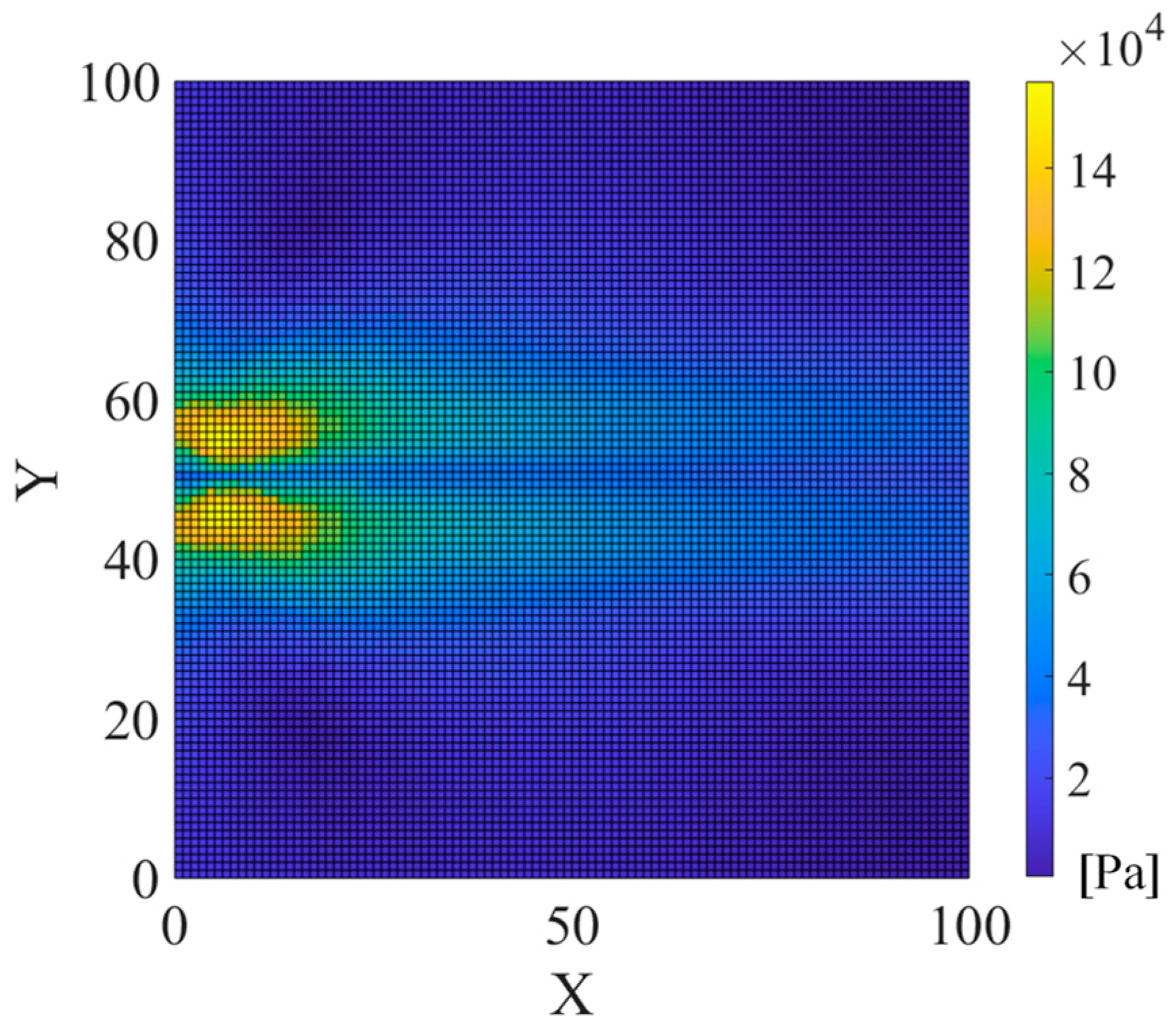
6.3. Intensity and Attenuation

Figure 13 shows the plot of the pressure pulsation peak-to-peak values ΔP (at 97% confidence intervals). In this study, it was used to monitor the spatial attenuation of the total pressure pulsation intensity including all of the frequency components. The pattern of ΔP was strongly similar to the pattern of f_vs amplitude. It was also symmetrically distributed (along Y = 50) under the influence of two-rows of local shedding vortex flow. This indicates that f_vs was, without a doubt, the most dominant frequency in the monitored region. However, there was also a difference between the ΔP pattern and the f_vs amplitude pattern in that the intensity of ΔP was not so weak in the X = 30~X = 90 region on the Y = 50 line. This was because of the existence of local high intensity component of 2 f_vs.

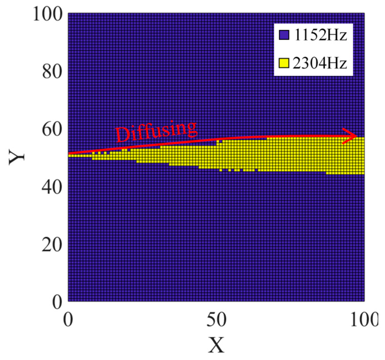
6.4. Dominant Frequency Distribution

The dominant frequency distribution, which is shown in Figure 14, was obtained by analysing the dominant frequency at every PTN point. The results show that there were only two dominant frequencies, which were 1152 Hz and 2304 Hz. As described above, the 1152 Hz was f_vs and is shown in blue. The 2304 Hz was 2 f_vs and is shown in yellow. It was found that the 2 f_vs frequency distribution was symmetrically diffused in a “jet-shape”. In detail, the 2 f_vs yellow region was very narrow (approximately ΔY = 2) on the trailing edge of the foil because the vortex shedding occurred locally on a one-by-one basis. However, it became increasingly wide along the flow direction due to the interaction between the two rows of vortexes. At X = 100, the width of 2 f_vs yellow region was approximately ΔY = 13. The diffusing ratio was initially quick but became slow after X > 50. Based on the interaction among the vortexes, as shown in Figure 7, the energy of the vortexes was also found to attenuate along the x-direction. for this reason, 2 f_vs became stronger, f_vs became weaker, and both f_vs and 2 f_vs were continually attenuating.

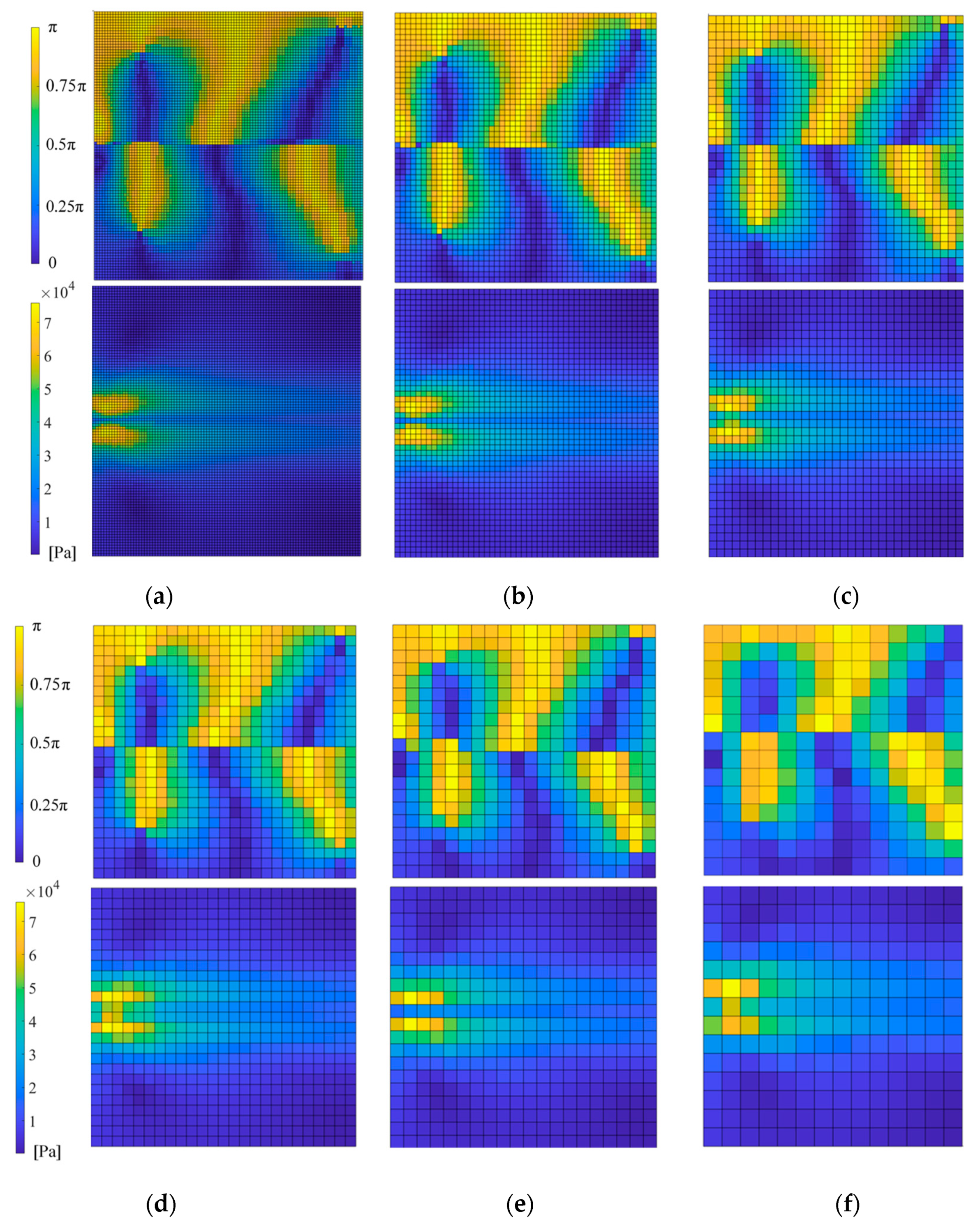
6.5. Phase and Phase Difference

The analysis of the phase and phase difference, based on PTN, demonstrated in this study represents breakthrough in terms of the understanding of pressure pulsation, as compared to traditional analysis. Firstly, it was necessary to set an initial reference point. In this case, the initial reference point P_ini was located on the centre of the trailing edge of the hydrofoil (X = 0, Y = 50), as illustrated. The phase of f_vs on the initial point was defined as the initial phase. The parameter Δφ represents the phase difference between any point and an initial point, and this is plotted in Figure 15a.

The above Figure shows an antiphase-symmetrical distribution from the blue-coloured to the yellow-coloured areas where the phase difference Δφ increased from 0 to π. in terms of the region between the Y = 50 line and Y = 80 line, as an example, it can be seen that Δφ decreased to 0 at approximately X = 20. The local low Δφ area (Δφ≈0) was distributed linearly as illustrated by red dash line. Then, Δφ increased from 0 to π. The X position, where Δφ = π on Y = 50 line, was approximately X = 46. However, Δφ = π was not linear, but had a curvilinear “S-shape”, as also illustrated. Then, Δφ decreased again to 0. The Δφ = 0 position on Y = 50 line was approximately X = 73. The local Δφ = 0 position became a more complex curve like “W-shape”. The transition from linear-shape to “S-shape” to “W-shape” shows that the flow regime became increasingly complex.

Taking Y = 20 line as another example, the distribution of Δφ is plotted in Figure 15b. Fitted by trend line, the X-Δφ relationship can be written as a polynomial formulation:

$$\Delta \phi ={\displaystyle \sum _{i=0}^6{C}_{xi}{X}^i}$$

(12)

where C_xi is the coefficient of the i-th order term. The values of C_xi are listed in

Table 3. The values of C_xi of the polynomial X-Δφ trend line.

Coefficient	Order of Polynomial Term	Value
Cx0	0	2.214 × 10−1
Cx1	1	4.896 × 10−2
Cx2	2	1.129 × 10−2
Cx3	3	−7.031 × 10−4
Cx4	4	1.412 × 10−5
Cx5	5	−1.165 × 10−7
Cx6	6	3.391 × 10−10

. The R² value of this fitting is approximately 0.913, which indicates goodness of fit. If Δφ = 0 is defined as a valley and Δφ = π is defined as a peak, the peak-valley distances along the x-direction are wider and wider. As shown, the ΔX values on the Y = 20 plot line between the peaks and valleys were approximately 21, 32 and 37 within X = 0~100. However, the increasing rate of ΔX became slower with the increasing of X. It is worth noting that this phenomenon may indicate the flow-wave attenuation.

7. Conclusions and Discussions

Based on CFD simulation and an experimental flow validation process, the pressure pulsation characteristics of tracking and processing in a hydrofoil trailing-edge vortex-shedding case, were shown. The following conclusions can be drawn:

(1)

CFD simulation with a proper time-frequency conversion algorithm, was shown to be effective in predicting the pulsation of turbulent flow fields. By setting discrete monitoring points on important sites, the dominant frequencies in a pulsation signal could be found. However, the traditional time-domain plot and frequency-domain plot were shown to be insufficient in terms of understanding the detailed influences of different pulsation frequencies. As an effective supplement, the pulsation tracking network (PTN) was helpful in resolving pulsating turbulent flow fields. The total pulsation intensity, dominant frequency, amplitude of frequencies, phase and phase difference could be well understood. The influence range, attenuation law and propagation law could be tracked. PTN was found to be very useful as a breakthrough in CFD post-processing.

(2)

In this study with a hydrofoil trailing-edge vortex-shedding flow case, PTN was proven to be effective in detailed analyses. Under the Reynolds number of 2.2 × 10⁶, the dominant frequencies were found to be f_vs = 1152 Hz and 2 f_vs = 2304 Hz. The highest amplitude regions of f_vs were symmetrically distributed because of the two shedding vortex rows. The highest amplitude region of 2 f_vs was slightly downstream to the trailing edge. It was caused by the interaction among vortexes. The f_vs frequency was dominant in most of the PTN monitored region. However, the f_vs intensity continually attenuated along x-direction with an increasingly wider 2 f_vs dominant region. The 2 f_vs frequency also attenuated along a fluctuating x-direction route. The phase difference contour and curves adequately proved the attenuation. The distances between peaks and valleys continually widened along the x-direction but this rate of increasing became slower over time.

Discussions are given as follows. In general, PTN was found to be much better than the traditional method in terms of analysing pulsating flow fields. Firstly, it accurately showed the sites with the strongest pulsation intensities, which may be missed in traditional analyses. For example, the maximum value of the RMS amplitude of f_vs was found to be less than 20,000 Pa according to the traditional method, but was actually found to be over 70,000 Pa when using PTN tracking. Secondly, unknown frequencies could be tracked by understanding their source, reason and attenuation. For example, in traditional analysis, f_vs and 2 f_vs can be only speculated upon as the relevant frequencies for vortex-shedding. By using PTN, the regions dominated by f_vs and 2 f_vs were found to overlap the positions of the shedding vortexes. The source, reason and attenuation of f_vs and 2 f_vs thus became much clearer. The spatial distribution of temporal states could be adequately shown. Thirdly, in future applications, the phase distribution will be useful in terms of solving actual engineering flow problems. The route in which the phase varies from 0 to π to 0 will indicate hidden directions of flow wave propagation.

References

- Mittal, S. Computation of three-dimensional flows past circular cylinder of low aspect ratio. Phys. Fluids 2001, 13, 177–191. [Google Scholar] [CrossRef]
- Voorhees, A.; Dong, P.; Atsavapranee, P.; Benaroya, H.; Wei, T. Beating of a Circular Cylinder Mounted as an Inverted Pendulum. J. Fluid Mech. 2008, 610, 217–247. [Google Scholar] [CrossRef]
- Wei, Z.; Zang, B.; New, T.H.; Cui, Y. A proper orthogonal decomposition study on the unsteady flow behaviour of a hydrofoil with leading-edge tubercles. Ocean Eng. 2016, 121, 356–368. [Google Scholar] [CrossRef]
- Towne, A.; Schmidt, O.T.; Colonius, T. Spectral proper orthogonal decomposition and its relationship to dynamic mode decomposition and resolvent analysis. J. Fluid Mech. 2018, 847, 821–867. [Google Scholar] [CrossRef] [Green Version]
- Hall, K.C.; Thomas, J.P.; Dowell, E.H. Proper Orthogonal Decomposition Technique for Transonic Unsteady Aerodynamic Plows. AIAA J. 2000, 38, 1853–1862. [Google Scholar] [CrossRef]
- Lumley, J.L. The structure of inhomogeneous turbulent flows. In Atmospheric Turbulence and Radio Wave Propagation; Nauka: Moscow, Russia, 1967; pp. 166–178. [Google Scholar]
- Hussain, A.K.M.F. Coherent structures in turbulence. J. Fluid Mech. 1986, 173, 303–356. [Google Scholar] [CrossRef]
- Hutchinson. Stochastic Tools in Turbulence; IOP Publishing Ltd.: Bristol, UK, 2007; Volume 22, p. 161. [Google Scholar]
- Sirovich, L. Turbulence and the Dynamics of Coherent Structures. I-Coherent Structures. II-Symmetries and Transformations. III-Dynamics and Scaling. Q. Appl. Math. 1987, 45, 561–571. [Google Scholar] [CrossRef] [Green Version]
- Jung, D. An Investigation of the Reynolds-Number Dependence of the Axisymmetric Jet Mixing Layer Using a 138 Hot-Wire Probe and the POD. Ph.D. Thesis, State University of New York at Buffalo, Buffalo, NY, USA, 2001. [Google Scholar]
- Berkooz, G.; Holmes, P.; Lumley, J.L. Lumley. The Proper Orthogonal Decomposition in the Analysis of Turbulent Flows. Annu. Rev. Fluid Mech. 1993, 25, 539–575. [Google Scholar] [CrossRef]
- Jo, T.; Koo, B.; Kim, H.; Lee, D.; Yoon, J.Y. Effective sensor placement in a steam reformer using gappy proper orthogonal decomposition. Appl. Therm. Eng. 2019, 154, 419–432. [Google Scholar] [CrossRef]
- Schmid, P.J. Dynamic mode decomposition of numerical and experimental data. J. Fluid Mech. 2010, 656, 5–28. [Google Scholar] [CrossRef] [Green Version]
- Schmid, P.J. Application of the dynamic mode decomposition to experimental data. Exp. Fluids 2011, 50, 1123–1130. [Google Scholar] [CrossRef]
- Kou, J.; Zhang, W. Dynamic mode decomposition and its application in fluid mechanics. Acta Aerodyn. Sin. 2018, 36, 163–179. [Google Scholar]
- Taira, K.; Brunton, S.L.; Dawson, S.T.; Rowley, C.W.; Colonius, T.; McKeon, B.J.; Schmidt, O.T.; Gordeyev, S.; Theofilis, V.; Ukeiley, L.S. Modal Analysis of Fluid Flows: An Overview. AIAA J. 2017, 55, 4013–4041. [Google Scholar] [CrossRef] [Green Version]
- Xue, D.; Pan, C.; Li, G. Measurement of tip vortex instability frequency based on flow visualization. J. Beijing Univ. Aeronaut. Astronaut. 2016, 42, 837–843. [Google Scholar]
- Dörfler, P.; Sick, M.; Coutu, A. Flow-Induced Pulsation and Vibration in Hydroelectric Machinery; Springer: Berlin/Heidelberg, Germany, 2013. [Google Scholar]
- Wylie, E.B.; Streeter, V.L. Fluid Transients; FEB Press: Ann Arbor, MI, USA, 1983. [Google Scholar]
- Chaudhry, M.H. Applied Hydraulic Transients; Van Nostrand Reinhold: New York, NY, USA, 1987. [Google Scholar]
- Shechtman, Y.; Eldar, Y.C.; Cohen, O.; Chapman, H.N.; Miao, J.; Segev, M. Phase retrieval with application to optical imaging. IEEE Signal Process. Mag. 2015, 32, 87–109. [Google Scholar] [CrossRef] [Green Version]
- International Electrotechnical Commission (IEC). Field Acceptance Tests to Determine the Hydraulic Performance of Hydraulic Turbines, Storage Pumps and Pump-Turbines; International Electrotechnical Commission (IEC): Geneva, Switzerland, 1991. [Google Scholar]
- Roth, S.; Calmon, M.; Farhat, M.; Muench, C.; Huebner, B.; Avellan, F. Hydrodynamic damping identification from an impulse response of a vibration blade. In Proceedings of the 3rd IAHR International Meeting of the Workgroup on Cavitation and Dynamic Problems in Hydraulic Machinery and Systems, Brno, Czech Republic, 14–16 October 2009. [Google Scholar]
- Ausoni, P. Turbulent Vortex Shedding from a Blunt Trailing Edge Hydrofoil. Ph.D. Thesis, Swiss Federal Institute of Technology Lausanne, Lausanne, Switzerland, 2009. [Google Scholar]
- Menter, F.R.; Kuntz, M.; Langtry, R. Ten years of industrial experience with the SST turbulence model. Turbul. Heat Mass Transf. 2003, 4, 625–632. [Google Scholar]
- Hellsten, A.; Laine, S. Extension of the k-ω-SST turbulence model for flows over rough surfaces. In Proceedings of the 22nd Atmospheric Flight Mechanics Conference, New Orleans, LA, USA, 11–13 August 1997. [Google Scholar]
- Huang, X.; Yang, W.; Li, Y.; Qiu, B.; Guo, Q.; Liu, Z. Review on the sensitization of turbulence models to rotation/curvature and the application to rotating machinery. Appl. Math. Comput. 2019, 341, 46–69. [Google Scholar] [CrossRef]
- Celik, I.B.; Ghia, U.; Roache, P.J.; Freitas, C.J. Procedure for estimation and reporting of uncertainty due to discretization in CFD applications. J. Fluids Eng. 2008, 130, 0780017. [Google Scholar]
- Zeng, Y.; Yao, Z.; Gao, J.; Hong, Y.; Wang, F.; Zhang, F. Numerical Investigation of Added Mass and Hydrodynamic Damping on a Blunt Trailing Edge Hydrofoil. J. Fluids Eng. 2019, 141, 0811088. [Google Scholar] [CrossRef]
- Vu, T.C.; Nennemann, B.; Ausoni, P.; Farhat, M.; Avellan, F. Unsteady CFD Prediction of Von Karman Vortex Shedding in Hydraulic Turbine Stay Vanes; Hydro: Granada, Spain, 2007. [Google Scholar]
- Kock, F.; Herwig, H. Local entropy production in turbulent shear flows: A high-Reynolds number model with wall functions. Int. J. Heat Mass Transf. 2004, 47, 2205–2215. [Google Scholar] [CrossRef]