On the Design of Power Law Filters and Their Inverse Counterparts

Abstract

This paper presents the optimal modeling of Power Law Filters (PLFs) with the low-pass (LP), high-pass (HP), band-pass (BP), and band-stop (BS) responses by means of rational approximants. The optimization is performed for three different objective functions and second-order filter mother functions. The formulated design constraints help avoid placement of the zeros and poles on the right-half s-plane, thus, yielding stable PLF and inverse PLF (IPLF) models. The performances of the approximants exhibiting the fractional-step magnitude and phase responses are evaluated using various statistical indices. At the cost of higher computational complexity, the proposed approach achieved improved accuracy with guaranteed stability when compared to the published literature. The four types of optimal PLFs and IPLFs with an exponent $\alpha$ of 0.5 are implemented using the follow-the-leader feedback topology employing AD844AN current feedback operational amplifiers. The experimental results demonstrate that the Total Harmonic Distortion achieved for all the practical PLF and IPLF circuits was equal or lower than 0.21%, whereas the Spurious-Free Dynamic Range also exceeded 57.23 and 54.72 dBc, respectively.

1. Introduction

The theoretical concepts of fractional calculus [1,2,3], which generalized differ-integral operators, have led to significant developments in circuit theory, signal processing, control theory, bio-impedance modeling, etc. [4,5,6,7,8]. Fractional-order (FO) filters are considered as the generalization of the traditional filters [9]. This is due to the ability of the FO filters to achieve any roll-off rate [10]; in contrast, an integer-order filter can only achieve a roll-off at $-20{log}_{10}n$ decibels/decade (dB/dec), where n is an integer [11]. FO analog filter transfer functions are generally realized from the integer-order filters by substitution of the Laplacian operator s with the non-integer Laplacian operator $s^{\alpha }$, where $\alpha \in (0,1).$ The frequency–domain transfer function of $s^{\alpha }$ is given by (1):

$${\left(j\omega \right)}^{\alpha }={\omega }^{\alpha }\left[cos\left(\frac{\alpha \pi }{2}\right)+jsin\left(\frac{\alpha \pi }{2}\right)\right],$$

(1)

where $j=\sqrt{-1}$ and $\omega$ is the angular frequency in radians per second (rad/s).

Since $s^{\alpha }$ is an irrational function, various rational approximations based on series truncation, frequency–domain curve-fitting, pole-zero placement, optimization techniques, etc., have been reported [12,13,14,15]. The impedance characteristics of the operator $s^{\alpha }$ may be practically realized using the FO elements (also known as the fractance devices or the constant phase elements) [16,17,18]. Due to the unavailability of the commercial FO device, their behavior may be emulated using the passive and active circuits [19,20,21,22].

Recent works have demonstrated the generalization of the Butterworth [23], Chebyshev [24], inverse Chebyshev [25], and elliptic filters [26] to the FO domain. Another design strategy that involves the approximation of FO filter characteristics using the integer order transfer function was also reported in the literature [27]. The integer order approximant can be realized using the field programmable analog array [28], voltage mode operational amplifier [29], switched capacitor [30], operational transconductance amplifier (OTA) [31], and current feedback operational amplifier (CFOA) [32].

The application of numerical and metaheuristic optimization algorithms for the approximation of FO filters has gained traction in recent years. The modeling of FO RLC filter and low-pass filter transfer functions of the form $1/{(s+1)}^{\alpha }$ using classical optimization techniques has been reported [33,34]. Numerical optimization methods were employed for the approximation of low-pass [35,36] and band-pass [37,38] filters exhibiting fractional-step behavior. The Nelder-Mead simplex [39], Cuckoo Search algorithm [40], and MATLAB-based optimization function fmincon [41,42] were employed to model the magnitude–frequency characteristics of the FO low-pass Butterworth filter. The performances of several nature-inspired algorithms were compared for the optimal rational approximation of the $s^{\alpha }$ operator [43]. The optimal design of a grounded FO inductor based on the generalized impedance converter was reported in [44]. $(1+\alpha )$ and $(\alpha +\beta )$ order, where $\alpha ,\beta \in (0,1)$, low-pass Bessel filter characteristics were optimally approximated using the Interior Search algorithm [45].

Since inverse filters yield the reciprocal frequency characteristic of the system that causes distortion during transmission or reception, these filters are widely used in communication systems to alleviate signal distortion [46]. Inverse filters are also employed in acoustic systems [47], proportional integral derivative controllers [48], and digital filtering [49]. Realizations of FO inverse filters using the operational amplifiers [50], CFOAs [51], operational trans-resistance amplifiers [52], and OTAs [53] have been recently reported.

A new class of FO filters, namely the Power Law Filter (PLF), was approximated based on a frequency–domain curve fitting using the Sanathanan–Koerner (S-K) least-square iterative method in [54]. Applications of power law compensators and filters in achieving robust frequency compensation of process plants with uncertainties [55] and in bio-impedance modeling of fruits [56] have also been exemplified. The transfer function, magnitude–frequency, and phase–frequency relationships for these filters exhibiting the low-pass (LP), high-pass (HP), band-pass (BP), and band-stop (BS) characteristics are presented in

Table 1. Transfer functions and frequency response expressions of the theoretical PLFs (${\omega }_0$: pole frequency, and Q: quality factor).

Type	Transfer Function	Magnitude	Phase
Low-pass	$H_{\mathrm{D}}^{\mathrm{LP}}\left(s\right)={\left(\frac{{\omega }_0^2}{s^2+\frac{{\omega }_0}{Q}s+{\omega }_0^2}\right)}^{\alpha }$	$\frac{1}{{\left[1+{\left(\frac{\omega }{{\omega }_0}\right)}^4+{\left(\frac{\omega }{{\omega }_0}\right)}^2·\left(\frac{1}{Q^2}-2\right)\right]}^{\alpha /\phantom{\alpha 2}2}}$	$-\alpha ·{tan}^{-1}\left[\frac{\left(\frac{\omega }{{\omega }_0}\right)·\frac{1}{Q}}{1-{\left(\frac{\omega }{{\omega }_0}\right)}^2}\right]$
High-pass	$H_{\mathrm{D}}^{\mathrm{HP}}\left(s\right)={\left(\frac{s^2}{s^2+\frac{{\omega }_0}{Q}s+{\omega }_0^2}\right)}^{\alpha }$	$\frac{{\left(\frac{\omega }{{\omega }_0}\right)}^{2\alpha }}{{\left[1+{\left(\frac{\omega }{{\omega }_0}\right)}^4+{\left(\frac{\omega }{{\omega }_0}\right)}^2·\left(\frac{1}{Q^2}-2\right)\right]}^{\alpha /\phantom{\alpha 2}2}}$	$\alpha ·\left\{\pi -{tan}^{-1}\left[\frac{\left(\frac{\omega }{{\omega }_0}\right)·\frac{1}{Q}}{1-{\left(\frac{\omega }{{\omega }_0}\right)}^2}\right]\right\}$
Band-pass	$H_{\mathrm{D}}^{\mathrm{BP}}\left(s\right)={\left(\frac{\frac{{\omega }_0}{Q}s}{s^2+\frac{{\omega }_0}{Q}s+{\omega }_0^2}\right)}^{\alpha }$	$\frac{\frac{1}{Q^{\alpha }}·{\left(\frac{\omega }{{\omega }_0}\right)}^{\alpha }}{{\left[1+{\left(\frac{\omega }{{\omega }_0}\right)}^4+{\left(\frac{\omega }{{\omega }_0}\right)}^2·\left(\frac{1}{Q^2}-2\right)\right]}^{\alpha /\phantom{\alpha 2}2}}$	$\alpha ·\left\{\frac{\pi }{2}-{tan}^{-1}\left[\frac{\left(\frac{\omega }{{\omega }_0}\right)·\frac{1}{Q}}{1-{\left(\frac{\omega }{{\omega }_0}\right)}^2}\right]\right\}$
Band-stop	$H_{\mathrm{D}}^{\mathrm{BS}}\left(s\right)={\left(\frac{s^2+{\omega }_0^2}{s^2+\frac{{\omega }_0}{Q}s+{\omega }_0^2}\right)}^{\alpha }$	$\frac{{\left[1-{\left(\frac{\omega }{{\omega }_0}\right)}^2\right]}^{\alpha }}{{\left[1+{\left(\frac{\omega }{{\omega }_0}\right)}^4+{\left(\frac{\omega }{{\omega }_0}\right)}^2·\left(\frac{1}{Q^2}-2\right)\right]}^{\alpha /\phantom{\alpha 2}2}}$	$-\alpha ·{tan}^{-1}\left[\frac{\left(\frac{\omega }{{\omega }_0}\right)·\frac{1}{Q}}{1-{\left(\frac{\omega }{{\omega }_0}\right)}^2}\right]$

[54]. In the PLFs, a FO exponent term $\alpha$ is introduced in the transfer function of the second-order filter (referred to as the mother filter function). Consequently, the second-order filter characteristics may now be considered as a particular case of the PLFs when $\alpha =1.$

This paper presents the optimal modeling of PLFs exhibiting the LP, HP, BP, and BS characteristics. Comparative studies concerning the modeling performance based on three different objective function formulations are presented. A non-parametric statistical null hypothesis test is employed to investigate the similarity in the design performances between the objective functions. The proposed strategy incorporates constraints to ensure a stable PLF approximant. Additional constraints are also incorporated to avoid the placement of zeros in the right-half s-plane. This allows the attainment of inverse PLF (IPLF) characteristics through inversion of the optimal PLF models. Although the S-K method [54] is simpler and computationally superior compared to the proposed technique, the suggested approach demonstrates the following advantages:

(i)

The stability of the PLF approximant in S-K method [54] is governed by the stability of the mother filter function. While this guarantees a stable rational approximant, however, the zeros of the filter transfer function may lie on the right-half of s (RHS)-plane. For example, while the zeros of the BPPLFs and BSPLFs designed using the S-K method lie on the left-half s-plane; however, the LPPLF and HPPLF models for $\alpha =0.7$ have zeros located at {+183.0053, –23.6922, –8.6177, –1.7485} and {+0.0055, –0.5718, –0.1161, –0.0422}, respectively. It may be noted that for the S-K method-based LPPLFs and HPPLFs with $\alpha \in [0.51,0.99]$, one zero lies on the RHS-plane. Consequently, inverting such a transfer function will lead to an unstable inverse-LPPLF (ILPPLF) and inverse-HPPLF (IHPPLF) model. In contrast, the proposed approach can guarantee the generation of stable designs for both PLFs and IPLFs. Hence, this paper also presents the design of IPLFs that has not yet been reported in the literature.

(ii)

The modeling accuracy of the proposed optimal PLF approximants, as justified by the Mean Absolute Relative Error (MARE) metric, is significantly better (particularly for the LP, HP, and BP-types) in comparison to the S-K method.

To demonstrate the practical efficacy, discrete component-based circuit realization using CFOAs as active elements for the proposed PLFs and their inverse counterparts with $\alpha =0.5$ is conducted. The experimental results reveal excellent agreement with the theoretical magnitude– and phase–frequency behavior for the PLFs and magnitude responses for the IPLFs. The time–domain and Fast Fourier Transformation (FFT) characteristics of the practical filters are also investigated.

In this paper, Section 2 presents the proposed optimization problem formulation and PLF/IPLF design strategy. The modeling accuracy of the proposed method is investigated using MATLAB simulations in Section 3. Statistical studies concerning the hypothesis test are also presented in this section. Practical circuit implementation and experimental results (magnitude–frequency, phase–frequency, time–domain, and FFT) for the designed filters are presented in Section 4. Finally, the paper concludes in Section 5.

2. Proposed Technique

The proposed rational approximant of the PLF is modeled as per (2):

$$H_{\mathrm{P}}\left(s\right)=\frac{a_N{s}^N+a_{N-1}{s}^{N-1}+\dots +a_{1}s+a_0}{s^N+b_{N-1}{s}^{N-1}+b_{N-2}{s}^{N-2}+\dots +b_{1}s+b_0},$$

(2)

where the coefficients of the numerator and denominator polynomials of $H_{\mathrm{P}}\left(s\right)$ are denoted by $a_k$ (k = 0, 1,…, N) and $b_k$ (k = 0, 1,…, N–1), respectively; and N is the order of the filter.

Figure 1 presents the flowchart of the proposed PLF design technique. The magnitude and phase characteristics of the PLFs may be approximated by determining the optimal values of the coefficients of $H_{\mathrm{P}}\left(s\right)$ such that the error between the theoretical and proposed responses is minimized. For this purpose, three different objective functions, as defined by (3)–(5), are proposed:

$$f_1=\frac{1}{L}\sum _{i=1}^L\left||20{log}_{10}\left|H_{\mathrm{D}}\left(j{\omega }_i\right)\right|-20{log}_{10}\left|H_{\mathrm{P}}(j{\omega }_i,X)\right|\right|+\frac{180}{\pi }\left|\angle H_{\mathrm{D}}\left(j{\omega }_i\right)-\angle H_{\mathrm{P}}(j{\omega }_i,X)\right|,$$

(3)

$$f_2=\frac{1}{L}\sum _{i=1}^L\left|\left|H_{\mathrm{D}}\left(j{\omega }_i\right)\right|-\left|H_{\mathrm{P}}(j{\omega }_i,X)\right|\right|+\left|\angle H_{\mathrm{D}}\left(j{\omega }_i\right)-\angle H_{\mathrm{P}}(j{\omega }_i,X)\right|,$$

(4)

$$f_3=\frac{1}{L}\sum _{i=1}^L\left|1-\frac{\left|H_{\mathrm{P}}(j{\omega }_i,X)\right|}{\left|H_{\mathrm{D}}\left(j{\omega }_i\right)\right|}\right|+\left|1-\frac{\angle H_{\mathrm{P}}(j{\omega }_i,X)}{\angle H_{\mathrm{D}}\left(j{\omega }_i\right)}\right|,$$

(5)

where L denotes the total number of logarithmically spaced sample points in the bandwidth of interest $\omega \in [{\omega }_{min},{\omega }_{max}]$ rad/s; the decision variables vector is represented by $X=$ [a${}_N$a${}_N$${}_{-1}$ … a${}_0$b${}_N$${}_{-1}$b${}_N$${}_{-2}$ … b${}_0$]; $\left|H_{\mathrm{D}}\left(j\omega \right)\right|$ and $\left|H_{\mathrm{P}}\left(j\omega \right)\right|$ denote the magnitude of the theoretical PLF and the proposed approximant, respectively; and the phase angles for the theoretical $(\angle H_{\mathrm{D}}\left(j\omega \right))$ and proposed $(\angle H_{\mathrm{P}}\left(j\omega \right))$ PLFs are expressed in radians.

To achieve a stable design, the inequality constraints as given by (6) are incorporated in the proposed optimization method:

$${\mathsf{\Delta }}_1,{\mathsf{\Delta }}_2,{\mathsf{\Delta }}_3,\cdots ,{\mathsf{\Delta }}_N>0,$$

(6)

where ${\mathsf{\Delta }}_1=b_{N-1}$, ${\mathsf{\Delta }}_2=\left|\begin{array}{cc}{b}_{N-1}& b_{N-3}\\ b_N& b_{N-2}\end{array}\right|$, ${\mathsf{\Delta }}_3=\left|\begin{array}{ccc}{b}_{N-1}& b_{N-3}& b_{N-5}\\ b_N& b_{N-2}& b_{N-4}\\ 0& b_{N-1}& b_{N-3}\end{array}\right|,$…,

${\mathsf{\Delta }}_N=\left|\begin{array}{ccccc}{b}_{N-1}& b_{N-3}& b_{N-5}& \cdots & 0\\ b_N& b_{N-2}& b_{N-4}& \cdots & 0\\ 0& b_{N-1}& b_{N-3}& ⋮& 0\\ ⋮& ⋮& ⋮& \ddots & ⋮\\ 0& 0& 0& 0& b_0\end{array}\right|$ represent the Hurwitz determinants [57], and $b_N=1$. The locations of zeros are also restricted to avoid the right-half s-plane by incorporating the constraints in (6) with $b_k$ substituted with $a_k$ (k = 0, 1, ⋯, N). Thus, the proposed formulation can be solved using a global search constrained optimization problem solver.

The transfer function of the proposed IPLFs can be obtained as $H_{\mathrm{I}}\left(s\right)={\left[H_{\mathrm{P}}\left(s\right)\right]}^{-1}$. As the value of $\alpha$ approaches 1, it is possible that the coefficients $a_N$ and $a_0$ of the optimal LPPLF and HPPLF, respectively, may attain a value of 0. The corresponding ILPPLF would possess one extra zero as compared to the number of poles, while the IHPPLF model will have a pole located at the origin of the s-plane.

To circumvent these particular issues, (i) the proposed ILPPLF transfer function may be represented as $p.H_{\mathrm{I}}\left(s\right)/(s+p)$, where p is a large positive number such as 200, 500, or 1000. The accuracy of approximation for the IPLFs increases as p is increased; and (ii) for the case when $a_0=0$ arises for the HPPLF, $a_0$ may be replaced by a small, positive number (q), for instance, smaller than 0.005. This technique allows the pole of the IHPPLF to be shifted away from the origin towards the left-half of the s-plane, thus, avoiding potential instability issues.

A numerical optimizer requires a user-supplied initial point for the decision variables at the start of the optimization procedure. Subsequently, the optimization algorithm iteratively minimizes the objective function by varying the decision variables. For solving a constrained optimization problem, an additional task of the optimizer is to satisfy the design constraints (i.e., generate a feasible solution). At the end of a single run of the optimization routine (when the maximum number of function evaluations or iterations or function tolerance value is reached), the optimal values of decision variables are obtained.

The final solution quality of a numerical optimization algorithm may be influenced by the choice of the initial point. For solving the global search optimization problems, identifying an appropriate initial point may not be easy. To circumvent this problem, a standard technique is to independently execute the optimization routine several times (iter${}_{\mathrm{m}}$) with randomly chosen initial points in each run. Hence, iter${}_{\mathrm{m}}$ number of near-global optimal solution vectors can be generated in this process. The best decision variables vector (X${}_{\mathrm{best}}$) is selected as the one that achieves the smallest error (MARE in the present case) from the iter${}_{\mathrm{m}}$ solutions. The previously-mentioned strategy is employed in this paper for the optimal modeling of PLFs.

3. MATLAB Simulations and Performance Analysis

The optimization procedures to minimize the objective functions (3)–(5) are implemented in MATLAB programming language using the function fmincon (algorithm: active-set) with the following parameter settings: maximum number of function evaluations = 50,000; maximum number of iterations = 50,000; and termination tolerance on the function value $={10}^{-10}$. In each trial run, the initial point for the decision variables vector is randomly chosen from a uniform distribution in the interval [0, 50]. For each design case, iter${}_{\mathrm{m}}=100$ independent trial runs of the optimization routine for each objective function are carried out.

Quantitative comparisons of the design accuracy are carried out based on the MARE metric as defined by (7):

$$\mathrm{MARE}=\frac{1}{L}\left[\sum _{i=1}^L\left|1-\frac{\left|H_{\mathrm{P}}\left(j{\omega }_i\right)\right|}{\left|H_{\mathrm{D}}\left(j{\omega }_i\right)\right|}\right|+\sum _{i=1}^L\left|1-\frac{\angle H_{\mathrm{P}}\left(j{\omega }_i\right)}{\angle H_{\mathrm{D}}\left(j{\omega }_i\right)}\right|\right].$$

(7)

For demonstration purposes, the values of L, $\alpha$, N, ${\omega }_{min}$, ${\omega }_{max}$, ${\omega }_0$, and Q are chosen as 1000, {0.3, 0.5, 0.7}, 4, 0.01 rad/s, 100 rad/s, 1 rad/s, and $1/\phantom{1\sqrt{2}}\sqrt{2}$, respectively. Detailed results for various other values of $\alpha$ are also available from the authors and can be shared with interested readers.

3.1. Statistical Analyses and Performance Evaluation

3.1.1. Comparisons Based on the MARE Metric

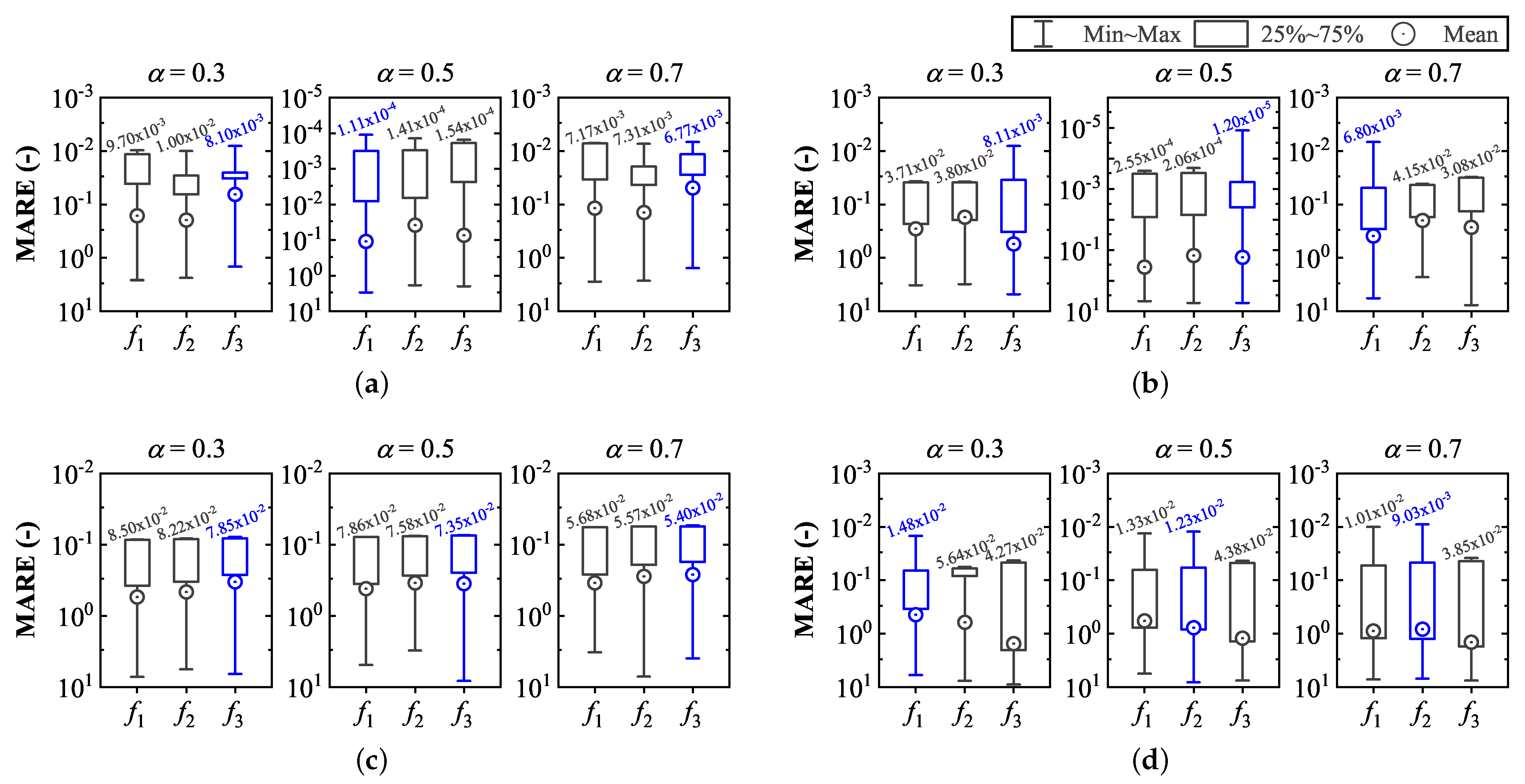
Statistical comparisons about the MARE metric were carried out to determine the average performance of the proposed optimization strategy for the design of PLFs using the three objective functions. The minimum (min), maximum (max), mean, and standard deviation (SD) indices for the various design orders are shown in

Table 2. Statistical comparisons of the MARE for designed PLFs.

Filter	Index		$\mathit{\alpha }=0.3$			$\mathit{\alpha }=0.5$			$\mathit{\alpha }=0.7$
		${\mathit{f}}_1$	${\mathit{f}}_2$	${\mathit{f}}_3$	${\mathit{f}}_1$	${\mathit{f}}_2$	${\mathit{f}}_3$	${\mathit{f}}_1$	${\mathit{f}}_2$	${\mathit{f}}_3$
LPPLF	Min	0.0097	0.0100	0.0081	1.11 $\times {10}^{-4}$	$1.41\times {10}^{-4}$	$1.54\times {10}^{-4}$	0.0072	0.0073	0.0068
	Max	2.6271	2.3788	1.4640	2.9436	1.8702	1.9990	2.7724	2.7217	1.5765
	Mean	0.1644	0.1960	0.0647	0.1095	0.0379	0.0740	0.1174	0.1410	0.0491
	SD	0.4655	0.4563	0.1877	0.4031	0.1910	0.3262	0.3996	0.3878	0.1707
HPPLF	Min	0.0371	0.0380	0.0081	$2.55\times {10}^{-4}$	$2.06\times {10}^{-4}$	$1.20\times {10}^{-5}$	0.0068	0.0415	0.0308
	Max	3.2533	3.0948	4.8429	4.7061	5.3711	5.3368	5.7460	2.2993	7.6727
	Mean	0.2869	0.1752	0.5542	0.3599	0.1516	0.1725	0.3906	0.1994	0.2710
	SD	0.5413	0.3953	0.9991	1.0042	0.6603	0.6509	0.8299	0.3567	0.9709
BPPLF	Min	0.0850	0.0822	0.0785	0.0786	0.0758	0.0735	0.0568	0.0557	0.0540
	Max	7.2483	5.6081	6.5838	4.9242	3.0704	8.2371	3.2517	7.1117	3.9668
	Mean	0.5429	0.4603	0.3324	0.4141	0.3461	0.3522	0.3440	0.2805	0.2651
	SD	0.9948	0.9361	0.7146	0.7051	0.5823	0.8862	0.6418	0.8186	0.5066
BSPLF	Min	0.0148	0.0564	0.0427	0.0133	0.0123	0.0438	0.0101	0.0090	0.0385
	Max	5.9545	7.6578	8.9775	5.6246	8.2135	7.5578	7.2166	7.0028	7.5591
	Mean	0.4435	0.6127	1.5306	0.5749	0.7712	1.2279	0.8967	0.8219	1.4433
	SD	0.9858	1.5685	2.1678	1.0939	1.5658	1.6760	1.6799	1.4094	1.8164

. Graphical comparisons for the MARE attained for the designed PLFs are presented using boxplots in Figure 2. In the case of LPPLFs, we found that: (i) for $\alpha =0.3$, $f_3$ attained the best performance for all the statistical indices; (ii) the most accurate model (i.e., the design with the minimum value of MARE (MARE${}_{\min }$)) for $\alpha =0.5$ was achieved by $f_1$ ($1.11\times {10}^{-4}$), although $f_2$ yielded the best results for the other indices; and (iii) very similar performances for MARE${}_{\min }$ were achieved for $\alpha =0.7$, with $f_3$ (0.0068) attaining marginally better accuracy.

However, $f_3$ distinctly outperformed the other two objective functions regarding the max, mean, and SD values. For the HPPLFs, (i) $f_3$ achieved significantly better MARE${}_{\min }$ (0.0081) as compared to $f_1$ (0.0371) and $f_2$ (0.0380) for $\alpha =0.3$. However, the max, mean, and SD performances for $f_3$ were the worst among the three functions; (ii) with $\alpha =0.5$, $f_1$ yielded inferior performance about the min, mean, and SD indices, while the best values concerning MARE${}_{\min }$ and mean MARE were achieved by $f_3$ ($1.20\times {10}^{-5}$) and $f_2$ (0.1516), respectively; and (iii) for $\alpha =0.7$, $f_1$ attained the most accurate model (MARE${}_{\min }$ = 0.0068), while $f_2$ yielded the best performance for all the other indices.

In the case of BPPLFs, it is revealed that: (i) for all the cases, the best performer about MARE${}_{\min }$ is $f_3$; (ii) regarding the mean and SD indices, $f_2$ attained the minimum value for $\alpha =0.5$ and $f_3$ for the other two orders; and (iii) the best results for the max MARE were achieved by $f_2$ (5.6081), $f_2$ (3.0704), and $f_1$ (3.2517) for $\alpha$ = 0.3, 0.5, and 0.7, respectively. Comparisons for the designed BSPLFs show that $f_1$ and $f_2$ achieved the best values for all the statistical indices with $\alpha =0.3$ and $\alpha =0.7$, respectively. In the case of $\alpha =0.5$, the most accurate model is attained by $f_2$ (MARE${}_{\min }$ = 0.0123), whereas $f_1$ yields superior performance for the other three indices.

3.1.2. Comparisons Based on the Wilcoxon Rank-Sum Hypothesis Test

Pair-wise comparisons based on the Wilcoxon rank-sum test for the PLFs designed using $f_1$, $f_2$, and $f_3$ are conducted to determine whether a statistically significant difference exists in the modeling performance [58]. If no significant difference exists in the design accuracy, then a similar average-case modeling error performance can be expected from all the proposed objective functions. Consequently, all the three objective functions may exhibit similar robustness.

Thus, in terms of solution consistency, the objective functions demonstrate similar performance. For this purpose, the null hypothesis (H${}_0$: ‘equality of medians for the MARE metric’) is considered at a confidence level of 95%. The decision index is represented by H, where H = 0/1 indicates that H${}_0$ cannot/can be rejected.

Table 3. Wilcoxon rank-sum test results for the designed PLFs.

Filter	Index		${\mathit{f}}_1$ vs. ${\mathit{f}}_2$			${\mathit{f}}_1$ vs. ${\mathit{f}}_3$			${\mathit{f}}_2$ vs. ${\mathit{f}}_3$
		$\mathit{\alpha }=0.3$	$\mathit{\alpha }=0.5$	$\mathit{\alpha }=0.7$	$\mathit{\alpha }=0.3$	$\mathit{\alpha }=0.5$	$\mathit{\alpha }=0.7$	$\mathit{\alpha }=0.3$	$\mathit{\alpha }=0.5$	$\mathit{\alpha }=0.7$
LPPLF	p-val	$3.3\times {10}^{-8}$	0.9173	$8.0\times {10}^{-9}$	$9.7\times {10}^{-4}$	0.0911	0.1443	$1.5\times {10}^{-6}$	0.0013	$1.4\times {10}^{-8}$
	H	1	0	1	1	0	0	1	1	1
HPPLF	p-val	0.7369	0.0303	$3.7\times {10}^{-6}$	0.5551	0.7966	$1.1\times {10}^{-8}$	0.2087	0.6574	$6.1\times {10}^{-6}$
	H	0	1	1	0	0	1	0	0	1
BPPLF	p-val	0.2503	0.0211	$8.8\times {10}^{-6}$	0.0474	0.0417	0.0322	0.1626	0.1416	0.8902
	H	0	1	1	1	1	1	0	0	0
BSPLF	p-val	$1.0\times {10}^{-6}$	$6.6\times {10}^{-4}$	$1.1\times {10}^{-4}$	0.0032	0.0294	0.0276	0.0087	0.1739	0.0708
	H	1	1	1	1	1	1	1	0	0

presents the Wilcoxon rank-sum test results along with the p-value (p-val) index. A smaller p-val indicates stronger evidence in favor of rejection of H${}_0$.

It is revealed that: (i) H${}_0$ is rejected for all the pair-wise combinations concerning the LPPLF, HPPLF, and BSPLF with $\alpha$ = 0.3, 0.7, and 0.3, respectively; (ii) only one case (HPPLF with $\alpha =0.3$) exists where all the combinations may result in non-rejection of H${}_0$; (iii) for comparisons involving all the three design orders for a particular pair, the hypothesis can be rejected for $f_1/f_2$ with the BSPLF, $f_2/f_3$ with the LPPLF, and $f_1/f_3$ for the BPPLF and BSPLF, whereas H${}_0$ may not be rejected for the BPPLF with $f_2/f_3$; and (iv) across all the PLFs, 9, 8, and 5 cases out of 12 exist for $f_1/f_2$, $f_1/f_3$, and $f_2/f_3$, respectively, that lead to the rejection of H${}_0$. Overall, it may be concluded from the statistical analysis that, in terms of attaining a similar performance consistency for all the design cases, the three objective functions cannot be used interchangeably.

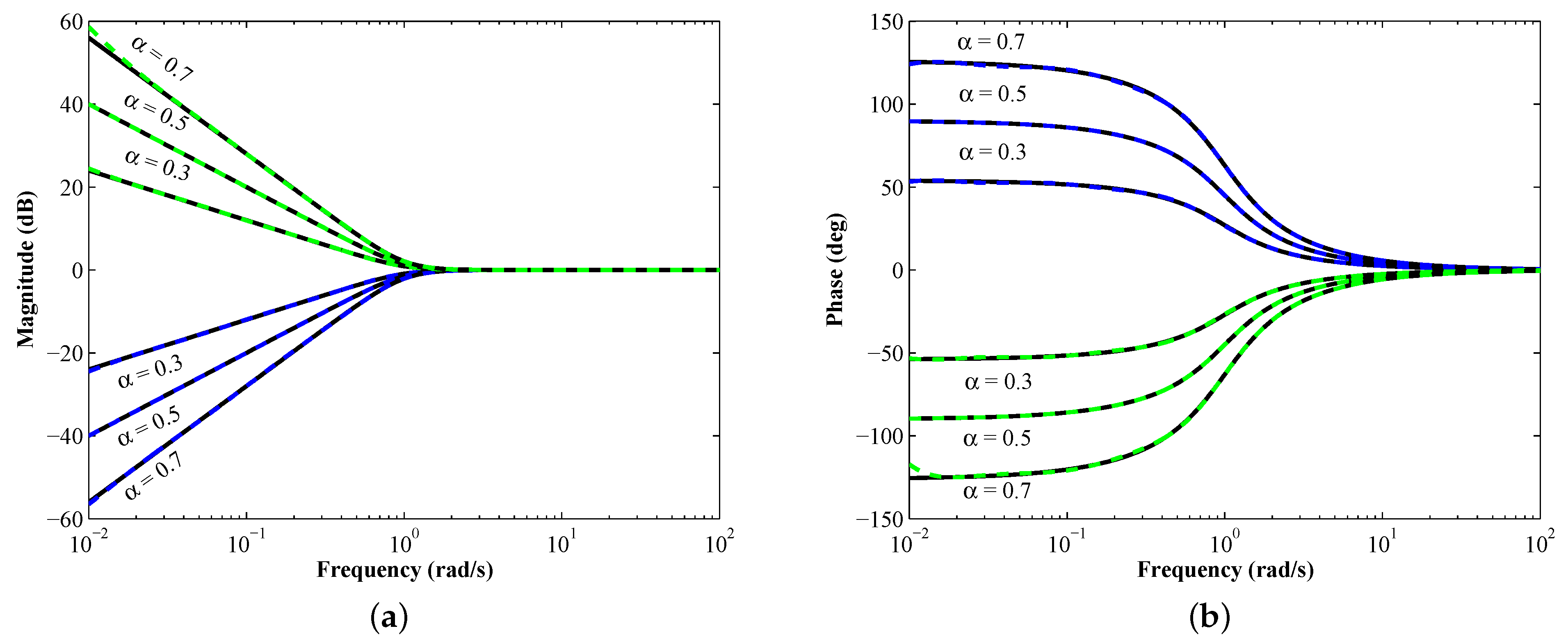
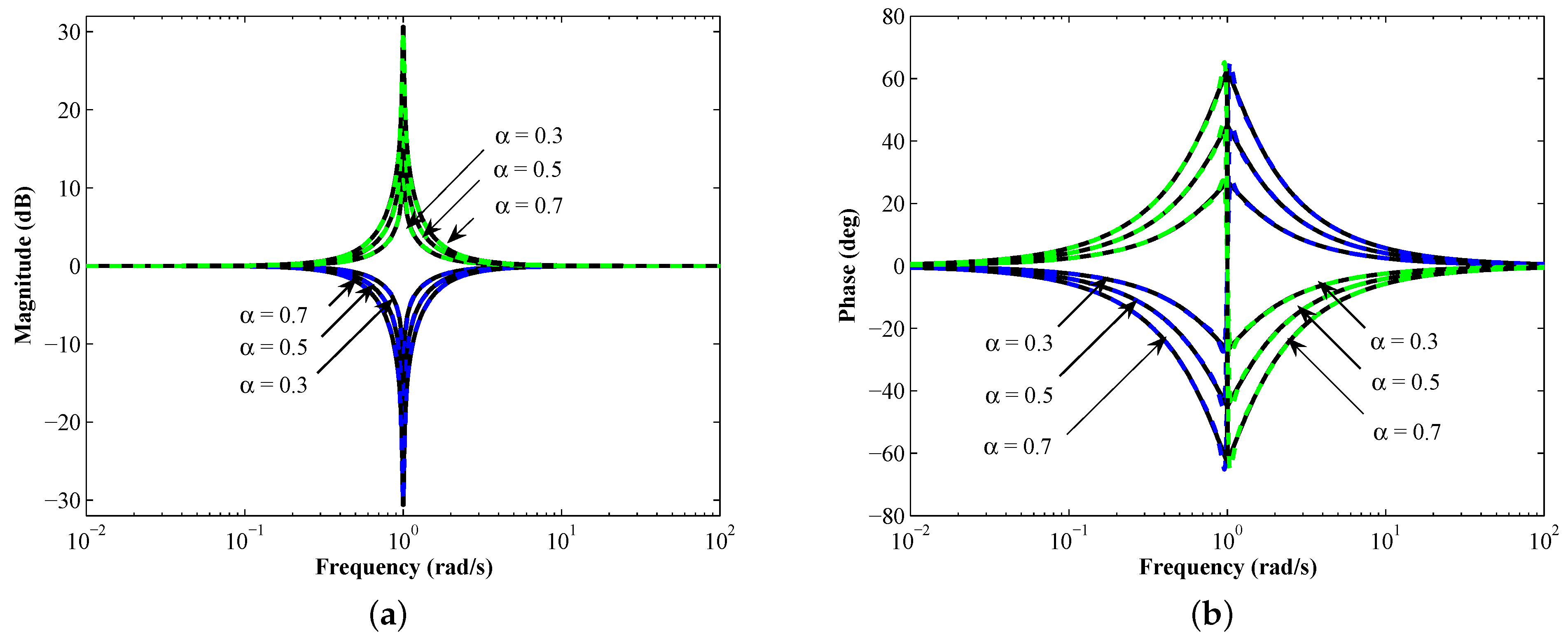
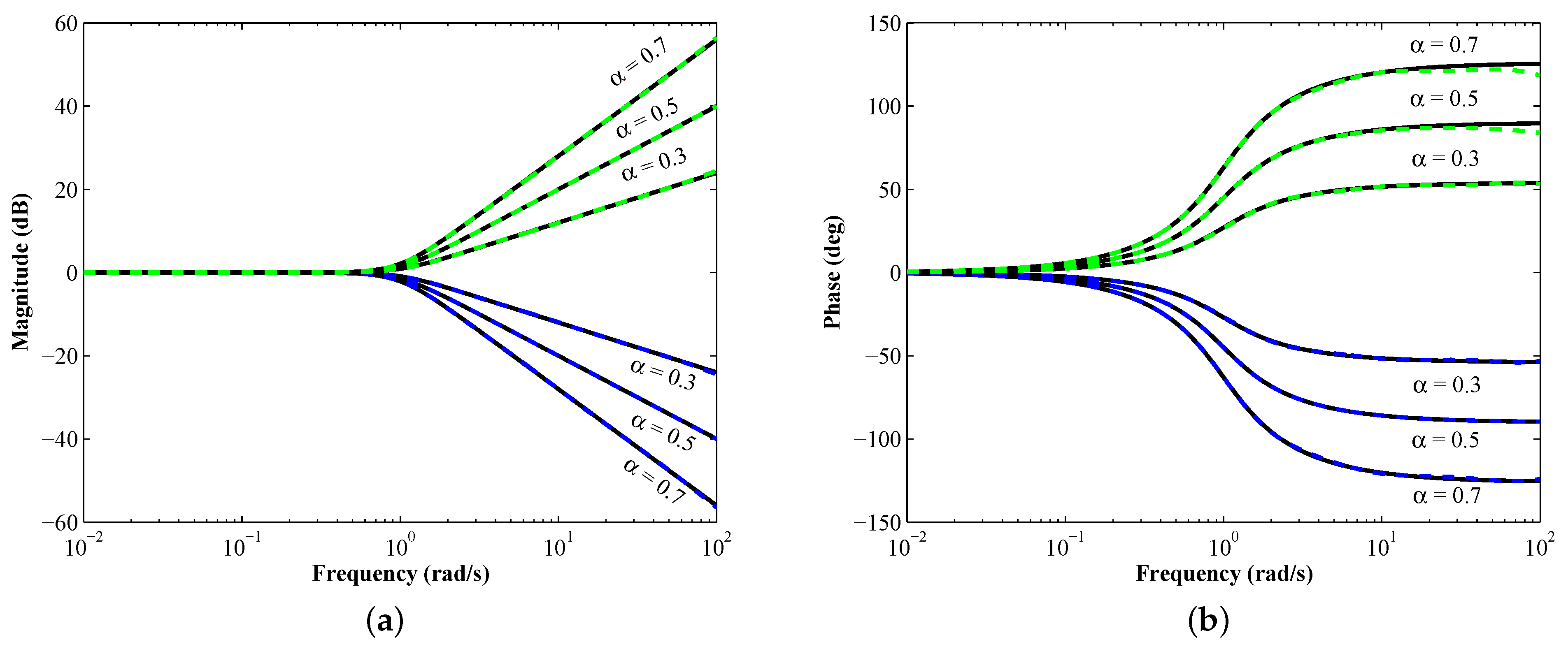
The optimal coefficients of the PLFs that achieve the smallest value of MARE for each of the three objective functions are presented in Appendix A. The MATLAB-simulated magnitude- and phase–frequency responses for the most accurate (least MARE${}_{\min }$) proposed LPPLFs, HPPLFs, BPPLFs, and BSPLFs are presented in Figure 3, Figure 4, Figure 5 and Figure 6, respectively. The plots for the corresponding IPLFs are also illustrated in these figures. The values of p and q are considered as 1000 and ${10}^{-6}$ for the ILPPLF and IHPPLF, respectively, for $\alpha =0.5$ and $0.7$. We observed that all the design cases attained good agreement with the theoretical responses.

The MARE${}_{\min }$ attained for the ILPPLF $(\alpha =0.5)$ with $p=\{100,200,500,1000\}$ is $\{0.0919,0.0439,0.0164,0.0079\}$. In the case of IHPPLF for $\alpha =0.5$ with $q=\{$0.005, 0.002, 0.001, 0.0001}, the MARE${}_{\min }$ is obtained as {0.0447, 0.0170, 0.0084, 0.0008}. These results confirm that the approximation accuracy of the ILPPLF and IHPPLF improves for larger values of p and smaller values of q, respectively. The MARE${}_{\min }$ attained for the proposed inverse BPPLFs (IBPPLFs) with $\alpha =\{0.3,0.5,0.7\}$ is {0.0790, 0.0745, 0.0548}; the same for the inverse BSPLFs (IBSPLFs) is $\{0.0147,0.0121,0.0092\}$.

3.2. Comparison with the Literature

The proposed most accurate PLFs are compared with the published literature [54] based on the MARE metric, as shown in

Table 4. Comparison of the most accurate proposed PLFs with the published literature [54] in terms of the MARE metric.

Filter	Reference	$\mathit{\alpha }=0.3$	$\mathit{\alpha }=0.5$	$\mathit{\alpha }=0.7$
LPPLF	[54]	0.0154	$2.68\times {10}^{-4}$	0.0410
	Proposed	0.0081	$1.11\times {10}^{-4}$	0.0068
HPPLF	[54]	0.0158	$9.39\times {10}^{-5}$	0.0410
	Proposed	0.0081	$1.20\times {10}^{-5}$	0.0068
BPPLF	[54]	0.0851	0.0884	0.0747
	Proposed	0.0785	0.0735	0.0540
BSPLF	[54]	0.0181	0.0138	0.0098
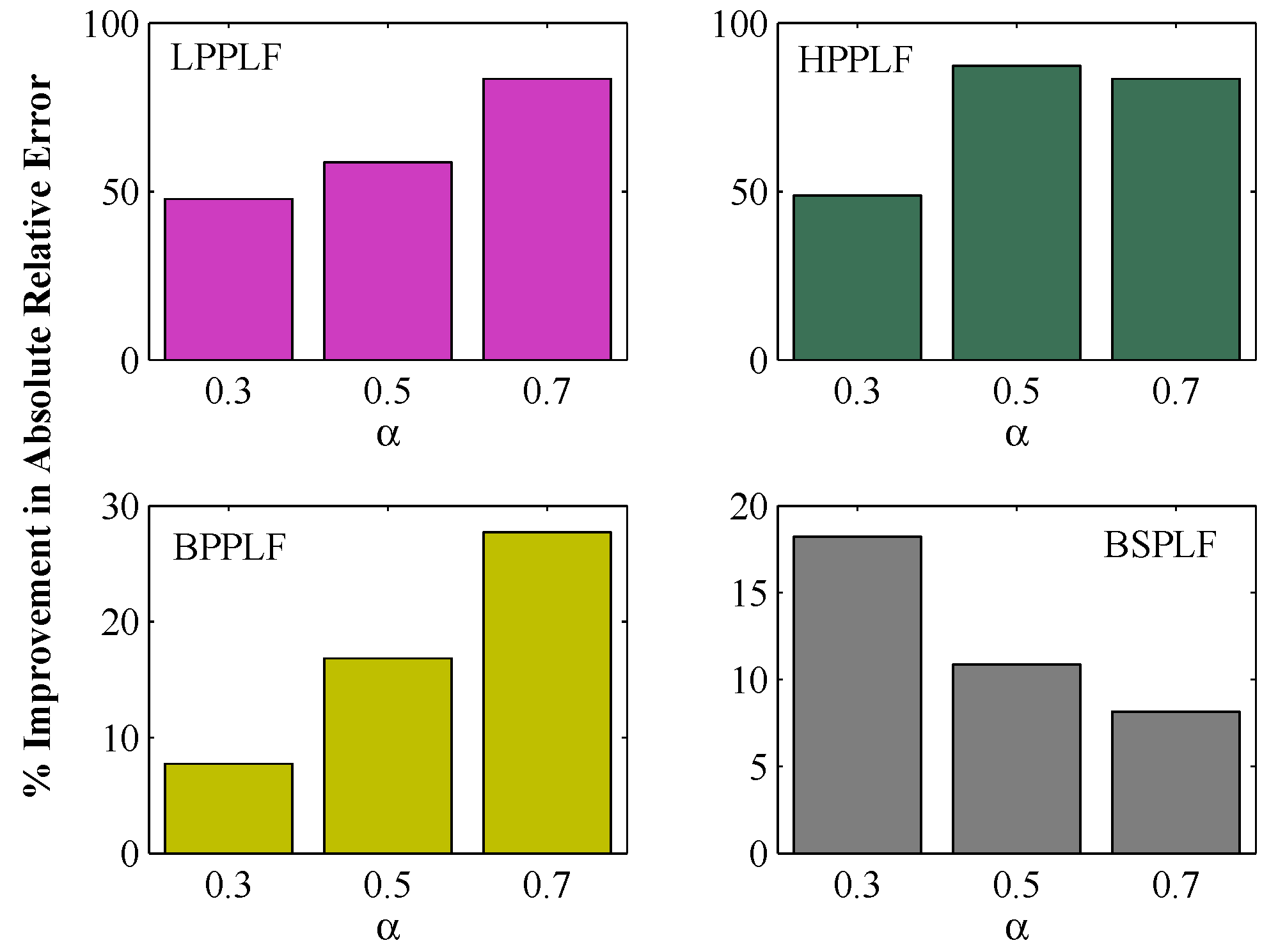
	Proposed	0.0148	0.0123	0.0090

. The proposed designs outperform the reported models for all the considered cases by achieving the least MARE values. The improvements in the percentage absolute relative error $(100\times \left|\frac{{\mathrm{MARE}}_{Prop}-{\mathrm{MARE}}_{Rep}}{{\mathrm{MARE}}_{Rep}}\right|)$, where ${\mathrm{MARE}}_{Prop}$ and ${\mathrm{MARE}}_{Rep}$ are the MARE values achieved for the proposed model and [54], respectively, for the LPPLF, HPPLF, BPPLF, and BSPLF with $\alpha =\{0.3,0.5,0.7\}$ are $\{47.40,58.58,83.41\}\%$, $\{48.73,87.22,83.41\}\%$, $\{7.75,16.85,27.71\}\%$, and $\{18.23,10.87,8.16\}\%$, respectively. Graphical visualizations of these percentage improvements for all the proposed designs are shown using bar plots in Figure 7. Improvements over [54] for the proposed LPPLF and HPPLF are distinctly pronounced as compared to those of the BPPLF and BSPLF. Hence, the proposed technique may be considered as a more accurate modeling tool when compared against [54].

Comparisons about the computational time ($t_{\mathrm{c}}$) required by the S-K method [54] and the proposed technique for the design of PLFs with $\alpha =0.5$ are conducted in the following environment—CPU: Intel i3 @ 1.70 GHz, RAM: 2.0 GB, Operating System: Windows 7 (64 bit), and Software: MATLAB 2014a. The $t_{\mathrm{c}}$ required by [54] for the design of LPPLF, HPPLF, BPPLF, and BSPLF is 1.601, 1.600, 1.665, and 1.663 s, respectively. For the proposed technique with objective functions $\{f_1,f_2,f_3\}$, the $t_{\mathrm{c}}$ (expressed in seconds) required to complete 100 iterations is, respectively, obtained as $\{254.036,230.221,215.673\}$, $\{251.964,213.028,260.650\}$, $\{265.070,296.818,291.986\}$, and $\{273.787,230.171,198.241\}$.

These results show that no specific objective function can attain the smallest value of $t_{\mathrm{c}}$ for all the designed PLFs. In terms of computational efficiency, the proposed strategy is inferior to the reported technique [54]. However, since the PLF approximation is carried out offline, the higher $t_{\mathrm{c}}$ of the proposed method may be traded-off in favor of achieving superior modeling accuracy compared to the S-K method [54].

4. Experimental Validation

CFOAs are popular analog signal processing integrated circuits that offer a high slew rate, gain-bandwidth decoupling, and smaller power consumption compared to operational amplifiers [59]. Due to their versatility, CFOAs have been widely employed to implement FO filters [19,32,41,51,60].

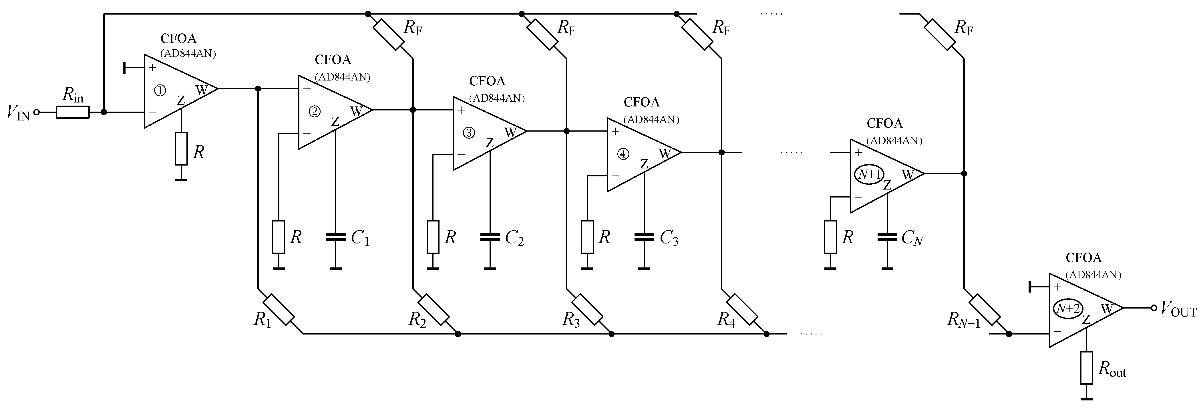
Discrete components-based circuit realization of the proposed PLFs is carried out by employing the CFOA as an active element in a follow-the-leader feedback topology [19]. The circuit diagram for the generalized PLF and IPLF implementation is presented in Figure 8. The total numbers of CFOAs, capacitors, and resistors required to realize the proposed Nth-order approximant are $N+2$, N, and $3N+4$, respectively.

The proposed circuit resulted in a reduced component count compared to [54] where the PLF implementation requires $N+4$ operational amplifiers, N capacitors, and $3N+8$ resistors. Thus, irrespective of the value of N, the circuit reported in [54] requires two extra op-amps and four additional resistors as compared to the proposed one. The general transfer function of the proposed circuit is given by (8):

$$\frac{V_{\mathrm{OUT}}\left(s\right)}{V_{\mathrm{IN}}\left(s\right)}=\frac{R_{\mathrm{out}}}{R_{\mathrm{in}}}\times \frac{{\displaystyle \frac{R}{R_1}{s}^N+\sum _{i=1}^N\frac{s^{N-i}}{{\displaystyle R_1{R}^{i-1}\prod _{k=1}^i\frac{R_{k+1}}{R_k}{C}_k}}}}{{\displaystyle s^N+\sum _{i=1}^N\frac{s^{N-i}}{{\displaystyle R_{\mathrm{F}}{R}^{i-1}\prod _{k=1}^i{C}_k}}}}.$$

(8)

As a representative, the circuit implementation steps for the proposed PLFs and IPLFs of LP, HP, BP, and BS types, whose transfer functions for $\alpha =0.5$ are given by (9)–(16), are presented below.

$$H_{\mathrm{P}}^{\mathrm{LP}}\left(s\right)=\frac{s^3+3.3454s^2+3.9298s+1.6952}{s^4+4.0523s^3+6.5467s^2+5.1288s+1.6952},$$

(9)

$$H_{\mathrm{P}}^{\mathrm{HP}}\left(s\right)=\frac{s^4+2.6111s^3+2.5477s^2+0.9238s}{s^4+3.3182s^3+4.6441s^2+3.2008s+0.9238},$$

(10)

$$H_{\mathrm{P}}^{\mathrm{BP}}\left(s\right)=\frac{0.0727s^4+8.6573s^3+56.5588s^2+8.6576s+0.0727}{s^4+26.6767s^3+58.9923s^2+26.6771s+1.0001},$$

(11)

$$H_{\mathrm{P}}^{\mathrm{BS}}\left(s\right)=\frac{0.9999s^4+0.6374s^3+2.0280s^2+0.6374s+1.0001}{s^4+1.3406s^3+2.2471s^2+1.3407s+1.0001},$$

(12)

$$H_{\mathrm{I}}^{\mathrm{LP}}\left(s\right)=\frac{200s^4+810.4600s^3+1309.3000s^2+1025.8000s+339.0400}{s^4+203.3454s^3+673.0098s^2+787.6552s+339.0400},$$

(13)

$$H_{\mathrm{I}}^{\mathrm{HP}}\left(s\right)=\frac{s^4+3.3182s^3+4.6441s^2+3.2008s+0.9238}{s^4+2.6111s^3+2.5477s^2+0.9238s+0.0020},$$

(14)

$$H_{\mathrm{I}}^{\mathrm{BP}}\left(s\right)=\frac{13.7552s^4+366.9422s^3+811.4484s^2+366.9477s+13.7565}{s^4+119.0825s^3+777.9752s^2+119.0867s+1},$$

(15)

$$H_{\mathrm{I}}^{\mathrm{BS}}\left(s\right)=\frac{1.0001s^4+1.3407s^3+2.2473s^2+1.3408s+1.0002}{s^4+0.6375s^3+2.0282s^2+0.6375s+1.0002}.$$

(16)

The design steps are described as follows:

Step 1:   

Set $N=4$ in (8). Therefore, six CFOAs, four capacitors, and 16 resistors are required to construct the circuit. The transfer function for the CFOA-based circuit is given by (17):

$$\frac{V_{\mathrm{OUT}}\left(s\right)}{V_{\mathrm{IN}}\left(s\right)}=\frac{R_{\mathrm{out}}}{R_{\mathrm{in}}}\times \frac{\frac{R}{R_1}{s}^4+\frac{s^3}{R_2{C}_1}+\frac{s^2}{R{R}_3{C}_1{C}_2}+\frac{s}{R^2{R}_4{C}_1{C}_2{C}_3}+\frac{1}{R^3{R}_5{C}_1{C}_2{C}_3{C}_4}}{s^4+\frac{s^3}{R_{\mathrm{F}}{C}_1}+\frac{s^2}{R{R}_{\mathrm{F}}{C}_1{C}_2}+\frac{s}{R^2{R}_{\mathrm{F}}{C}_1{C}_2{C}_3}+\frac{1}{R^3{R}_{\mathrm{F}}{C}_1{C}_2{C}_3{C}_4}}.$$

(17)

Step 2:

Select the desired center frequency for the filter. For instance, a center frequency of 1 kHz is used here.

Step 3:

Set the values of R, R${}_{\mathrm{F}}$, $R_{\mathrm{out}}$, and $R_{\mathrm{in}}$. Note that the resistor ratio $R_{\mathrm{out}}/R_{\mathrm{in}}$ helps in gain adjustment.

Step 4:

Compare the coefficients of (17) with the corresponding coefficients of the de-normalized transfer functions from (9)–(16) and determine the values of the remaining passive components for the filter.

Step 5:

Choose the nearest values of the passive components from the E24 industrial series for the resistors and the E12 series for the capacitors. The passive components required to implement the proposed PLFs and IPLFs are presented in

Table 5. Values of the passive components for the realization of the proposed PLFs $(\alpha =0.5)$ (Note: All resistances are in $\mathrm{k}\mathsf{\Omega }$, and all capacitances are in nF).

Filter	${\mathit{R}}_{\mathbf{out}}$	${\mathit{R}}_{\mathbf{in}}$	R	${\mathit{R}}_{\mathbf{F}}$	${\mathit{R}}_1$	${\mathit{R}}_2$	${\mathit{R}}_3$	${\mathit{R}}_4$	${\mathit{R}}_5$	${\mathit{C}}_1$	${\mathit{C}}_2$	${\mathit{C}}_3$	${\mathit{C}}_4$
LPPLF	10	10	10	10	∞	39	20	13	10	3.9	10	22	47
HPPLF	10	10	10	10	10	13	18	36	∞	4.7	12	22	56
BPPLF	10	10	10	10	130	30	10	30	130	0.56	6.8	33	390
BSPLF	10	10	10	10	10	20	11	20	10	12	10	27	22

and

Table 6. Values of the passive components for the realization of the proposed IPLFs $(\alpha =0.5)$ (Note: All resistances are in $\mathrm{k}\mathsf{\Omega }$, and all capacitances are in nF).

Filter	${\mathit{R}}_{\mathbf{out}}$	${\mathit{R}}_{\mathbf{in}}$	R	${\mathit{R}}_{\mathbf{F}}$	${\mathit{R}}_1$	${\mathit{R}}_2$	${\mathit{R}}_3$	${\mathit{R}}_4$	${\mathit{R}}_5$	${\mathit{C}}_1$	${\mathit{C}}_2$	${\mathit{C}}_3$	${\mathit{C}}_4$
ILPPLF	30	20	20	20	0.1	5.1	10	15	20	0.039	2.2	6.8	18
IHPPLF	11.5	10	200	200	200	160	110	56	0.43	0.33	0.82	2.2	390
IBPPLF	51	51	51	51	3.6	16	51	16	3.6	0.027	0.47	22	390
IBSPLF	51	51	51	51	51	24	47	24	51	4.7	1.0	10	2.2

, respectively. For better accuracy, $R_{\mathrm{out}}$ was selected from the E48 series for the IHPPLF.

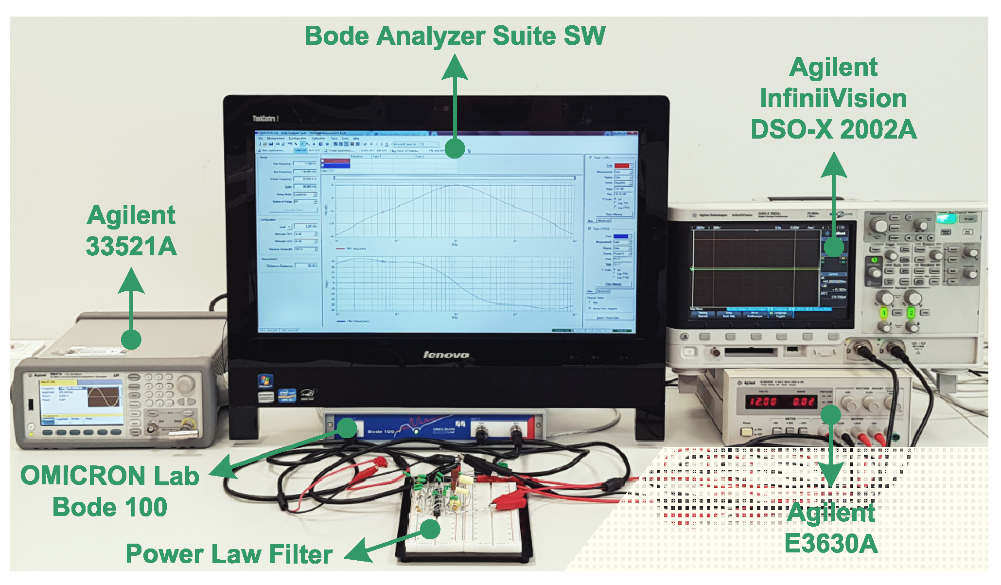
Practical circuit implementations were carried out using the Analog Devices AD844AN-type CFOAs. Supply voltage of 12 volts for the chips was provided from the Agilent E3630A power supply. The magnitude–frequency and phase–frequency measurements were conducted using the OMICRON Lab Bode 100 network analyzer and displayed using the Bode Analyzer Suite software. In this regard, 801 logarithmically spaced frequency points in the range 10 Hz to 100 kHz were considered. The level of the testing harmonic signal was set to V${}_{\mathrm{PP}}=1\mathrm{V}$.

The receiver bandwidth of the analyzer was fixed at 100 Hz. The time–domain behaviors of the practical filters were observed on Agilent InfiniiVision DSO-X 2002A digital storage oscilloscope. The voltage 1 V${}_{\mathrm{PP}}$ (default value) was applied to the filter circuit from the Agilent 33521A function/arbitrary waveform generator during measurements of time–domain responses. Figure 9 presents the photograph of the hardware set-up used to experimentally validate the performance of the proposed filters with the display demonstrating the frequency responses for the BPPLF as a test case.

4.1. Measurement Results for the PLFs

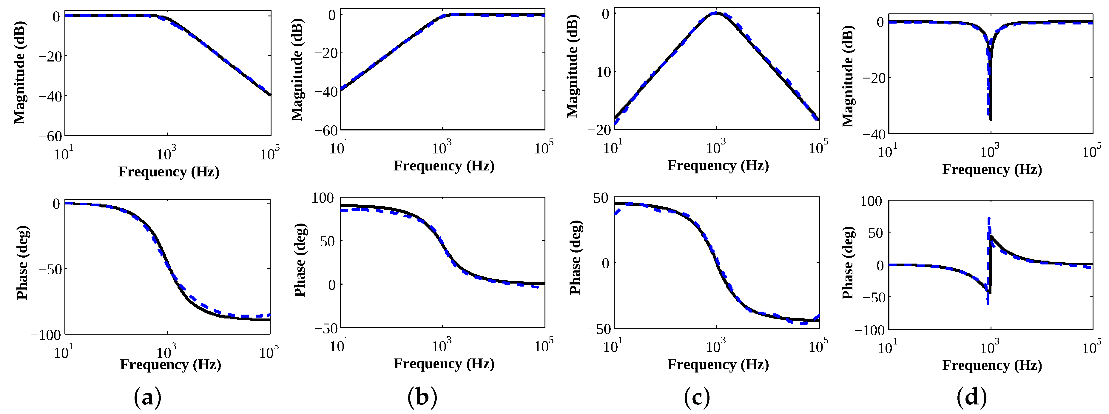
The experimentally obtained magnitude and phase characteristics for the proposed LPPLF, HPPLF, BPPLF, and BSPLF are compared with the theoretical ones in Figure 10a–d, respectively. All the cases achieve excellent agreement with the ideal responses. The MARE values (determined using $L=801$) attained for the practical PLFs exhibiting the LP, HP, BP, and BS behaviors are 0.1006, 0.9668, 0.1307, and 1.0031, respectively.

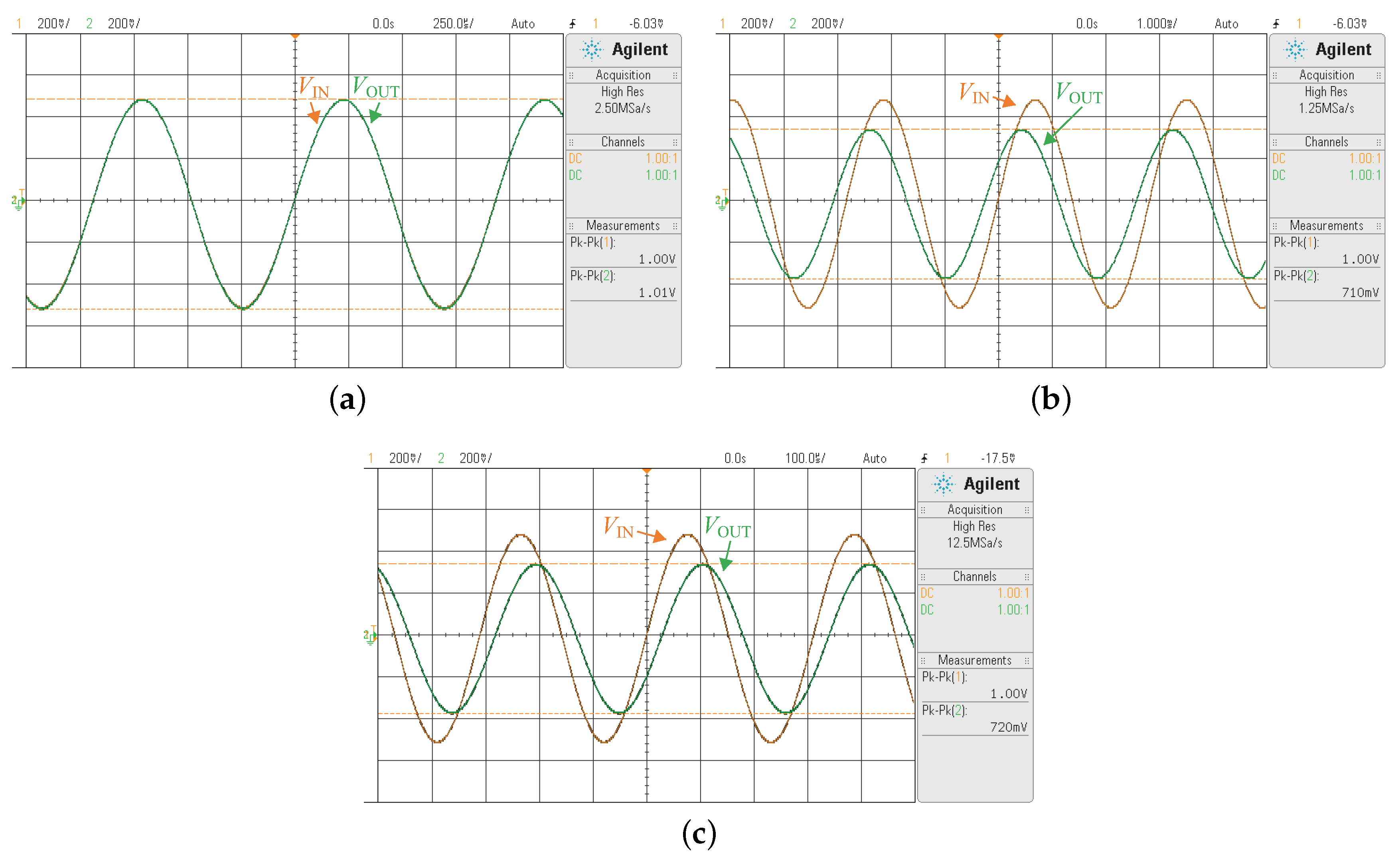
The time–domain responses of the proposed LPPLF and HPPLF measured at the half-power frequency ($f_{\mathrm{H}}$) of 1.11 kHz and 738 Hz, respectively, are shown in Figure 11a,b, respectively. The peak-to-peak output voltage (V${}_{\mathrm{OUT}\left(\mathrm{PP}\right)}$) obtained for the LPPLF and HPPLF at $f_{\mathrm{H}}$ are 700 mV and 680 mV, respectively. Figure 12a–c show the three time–domain input–output waveforms for the BPPLF (namely, BPPLF-a, BPPLF-b, and BPPLF-c) when the input signal is applied at the center frequency ($f_0=1.066$ kHz), low half-power frequency ($f_{\mathrm{H},\mathrm{low}}=353.9$ Hz), and high half-power frequency ($f_{\mathrm{H},\mathrm{high}}=3.214$ kHz), respectively.

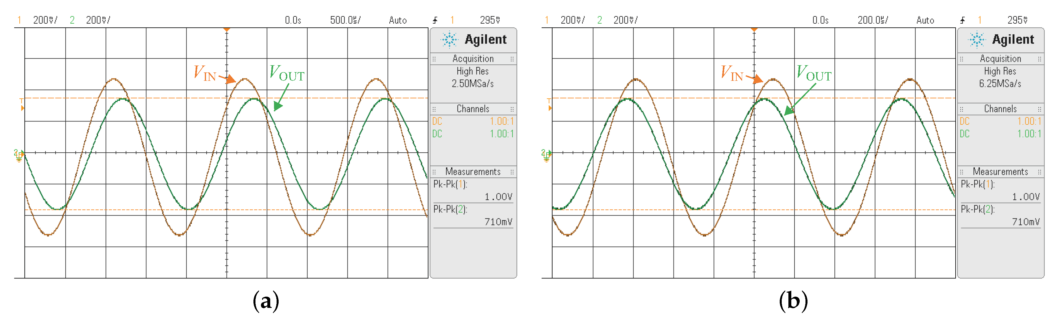
The corresponding values of V${}_{\mathrm{OUT}\left(\mathrm{PP}\right)}$ are attained as 1.01 V, 710 mV, and 720 mV, respectively. In Figure 13a,b, the two transient responses for the BSPLF (namely, BSPLF-a, and BSPLF-b) at the input signal frequencies of $f_{\mathrm{H},\mathrm{low}}$ (614 Hz) and $f_{\mathrm{H},\mathrm{high}}$ (1.47 kHz), respectively, are presented. Both cases yield 710 mV for V${}_{\mathrm{OUT}\left(\mathrm{PP}\right)}$. The values for $f_0$, $f_{\mathrm{H}}$, $f_{\mathrm{H},\mathrm{low}}$ and $f_{\mathrm{H},\mathrm{high}}$ are considered with respect to the experimental measurements.

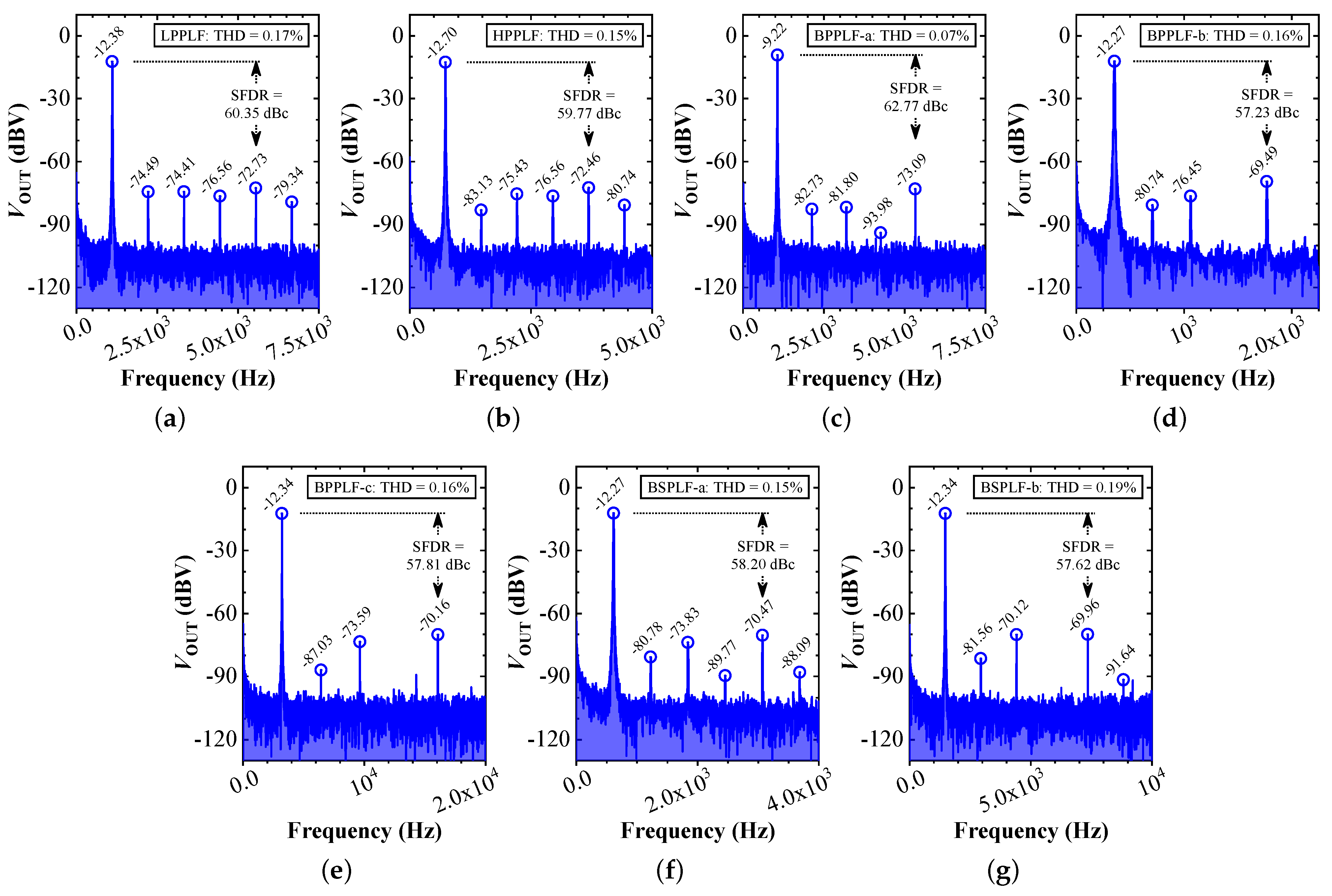
The Fourier spectrums of the measured output signals displayed up to the sixth harmonic above −95 dBV for the LPPLF, HPPLF, BPPLF-a, BPPLF-b, BPPLF-c, BSPLF-a, and BSPLF-b are shown in Figure 14a–g, respectively. The Spurious-Free Dynamic Range (SFDR), expressed in dBc, for the seven cases is respectively obtained as 60.35, 59.77, 62.77, 57.23, 57.81, 58.20, and 57.62. The Total Harmonic Distortion (THD), evaluated from the plotted harmonics, is obtained as 0.17%, 0.15%, 0.07%, 0.16%, 0.16%, 0.15%, and 0.19%.

4.2. Measurement Results for the IPLFs

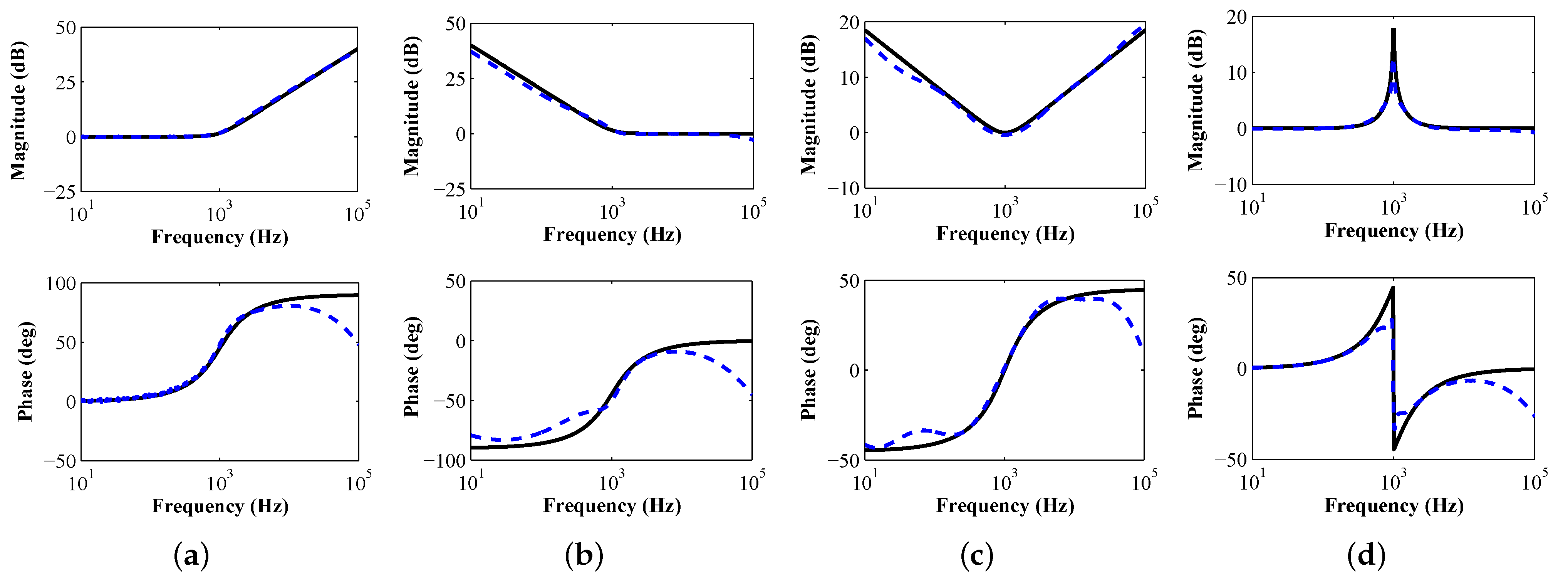
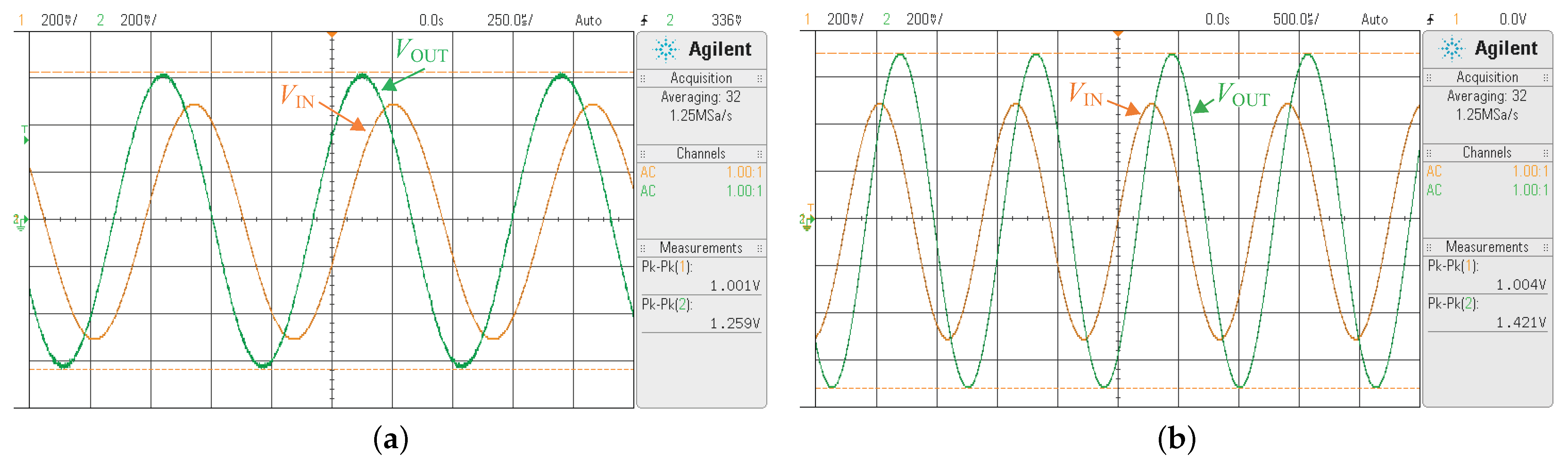
Comparisons between the theoretical and experimental magnitude and phase responses achieved for the proposed ILPPLF, IHPPLF, IBPPLF, and IBSPLF are presented in Figure 15a–d, respectively. The magnitude characteristics for all the cases demonstrate good agreement with the theoretical ones whereas the phase behavior deviates as the operating frequency approaches towards 100 kHz. The practical IPLFs with LP, HP, BP, and BS responses attain the MARE values of 0.2441, 6.8457, 0.2221, and 3.6490, respectively.

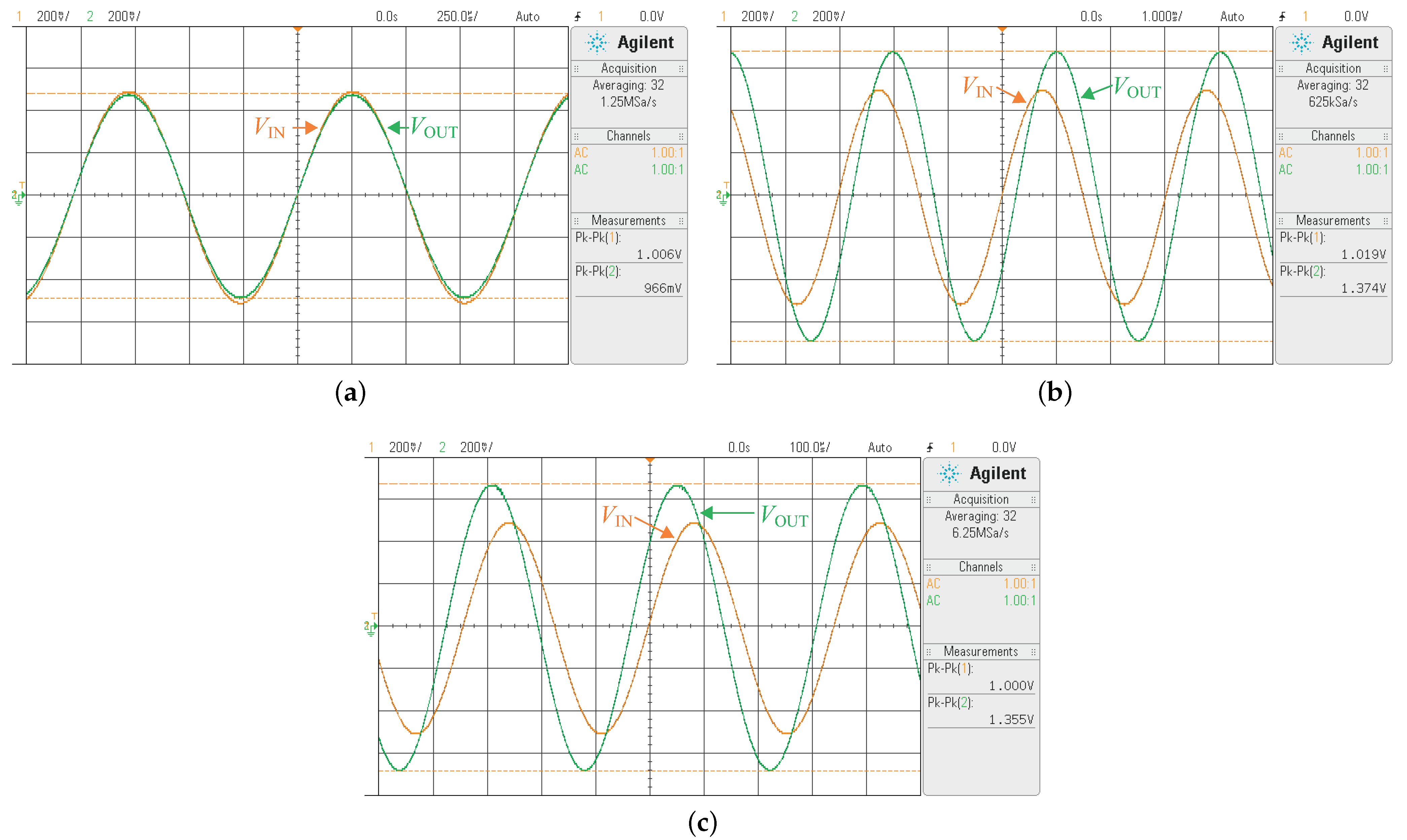
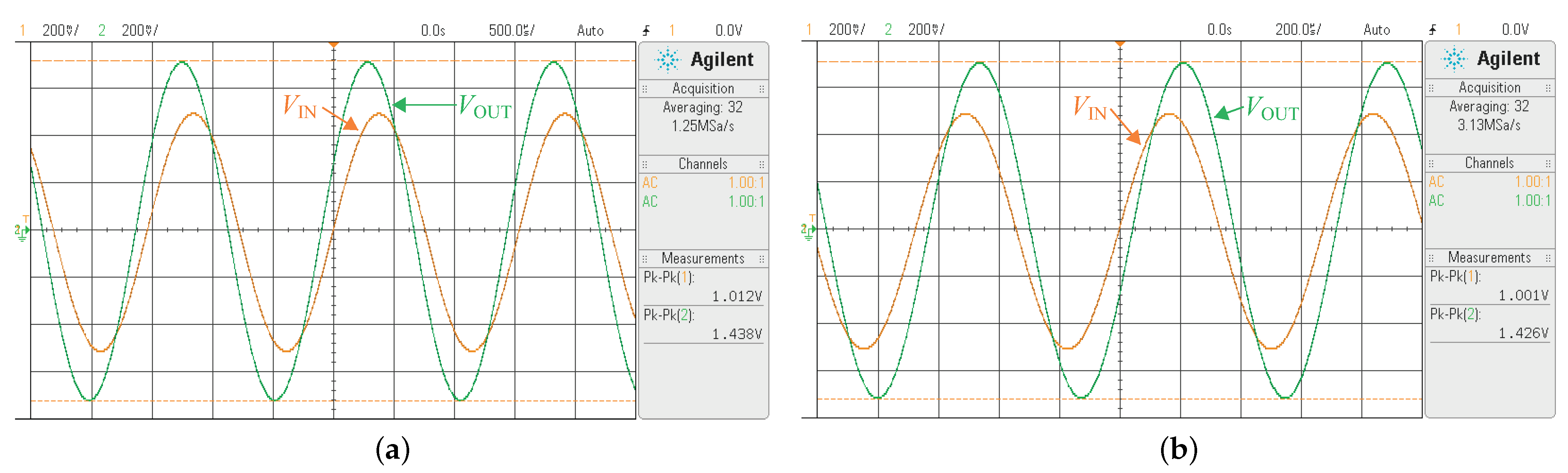
Figure 16a,b show the time–domain input–output waveforms of the practical ILPPLF and IHPPLF measured at the input frequency of $f_{\mathrm{H}}$ = 1.212 kHz and 887.8 Hz, respectively. Measurements reveal that $V_{\mathrm{OUT}\left(\mathrm{PP}\right)}$ of 1.259 V and 1.421 V are, respectively, obtained for the ILPPLF and the IHPPLF. The time–domain responses for the IBPPLF (i.e., IBPPLF-a, IBPPLF-b, and IBPPLF-c) at the input frequencies of $f_0$ = 967 Hz, $f_{\mathrm{H},\mathrm{low}}$ = 330.3 Hz, and $f_{\mathrm{H},\mathrm{high}}$ = 2.919 kHz are presented in Figure 17a–c. The values of $V_{\mathrm{OUT}\left(\mathrm{PP}\right)}$ achieved for these three cases are 0.966 V, 1.374 V, and 1.355 V, respectively. The input–output plots for the IBSPLF (i.e., IBSPLF-a and IBSPLF-b) at the input frequencies of $f_{\mathrm{H},\mathrm{low}}$ = 650.3 Hz and $f_{\mathrm{H},\mathrm{high}}$ = 1.482 kHz are shown in Figure 18a,b, respectively. The measured values of $V_{\mathrm{OUT}\left(\mathrm{PP}\right)}$ at these two frequencies are obtained as 1.438V and 1.426 V, respectively.

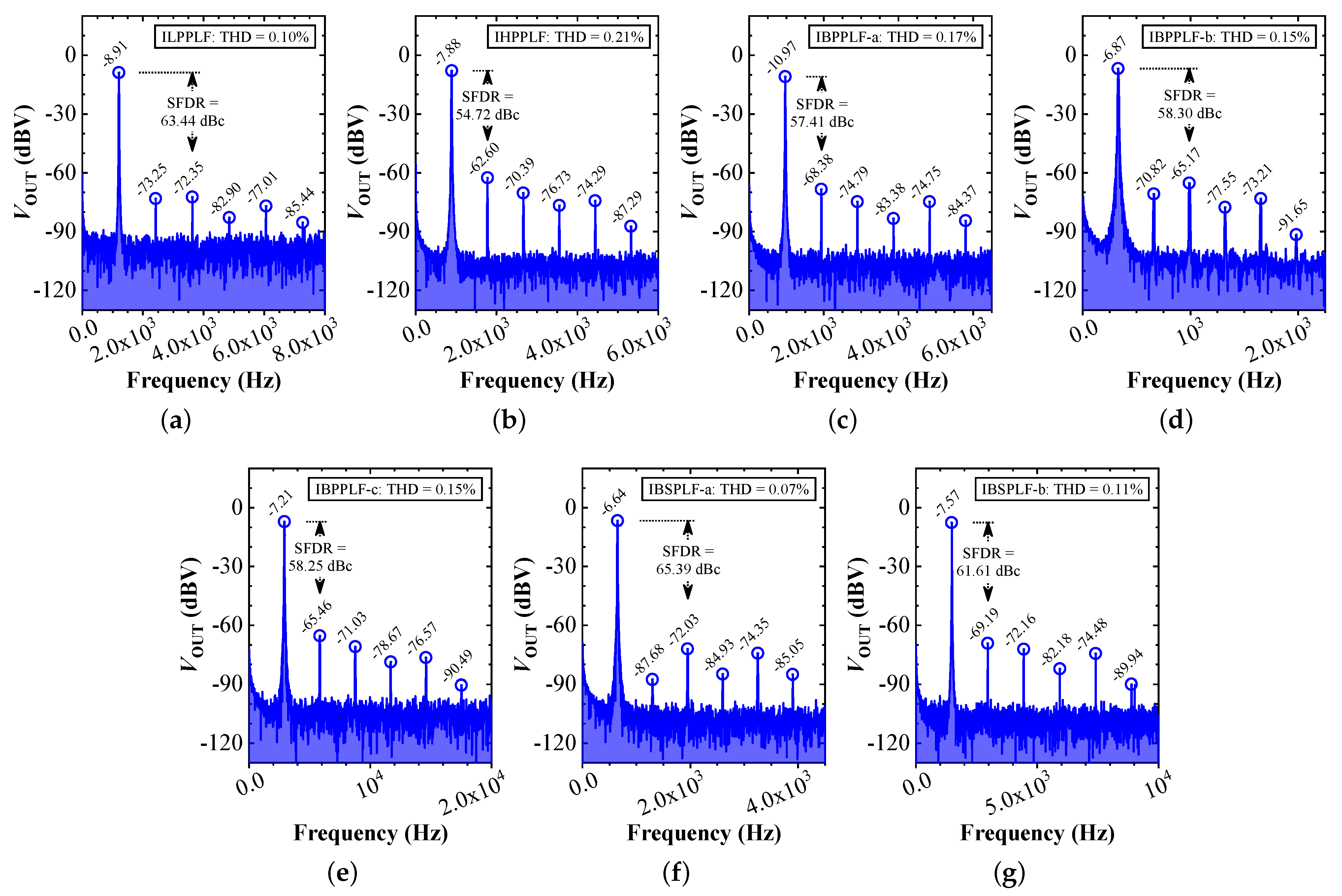
Figure 19a–g present the FFT plots of the measured output responses for the proposed ILPPLF, IHPPLF, IBPPLF-a, IBPPLF-b, IBPPLF-c, IBSPLF-a, and IBSPLF-b. The SFDR (dBc) attained for these designs is 63.44, 54.72, 57.41, 58.30, 58.25, 65.39, and 61.61; the corresponding THD values are 0.10%, 0.21%, 0.17%, 0.15%, 0.15%, 0.07%, and 0.11%.

5. Conclusions

In this paper, we presented the optimal and stable rational approximation of the PLFs and their inverse functions. Design examples for the LP, HP, BP, and BS-type PLFs with $\alpha$ = {0.3, 0.5, 0.7} and three different objective functions were presented. Statistical performance comparisons and Wilcoxon rank-sum test results revealed that no single objective function attained the best accuracy and solution quality consistency for all types of PLFs. Comparisons with published literature highlighted the improved accuracy for all the proposed PLFs. The drawback of obtaining unstable ILPPLF and IHPPLF for several design orders based on the reported S-K method was circumvented here through the incorporation of design constraints.

Since the PLF/IPLF design is an offline procedure, the inferior computational time of the proposed technique may be waived in favor of attaining the previously-mentioned benefits. CFOAs employed as active elements were used to practically realize the proposed PLFs and IPLFs for all four response types with $\alpha =0.5$. The experimental results exemplified an excellent agreement in the magnitude and phase responses with the ideal PLFs. The magnitude behavior for the IPLFs also attained proximity with the theoretical anticipations. For all measurements, the THD remained lower than 0.2%, and the SFDR exceeded 57.23 dBc for the PLFs. In the case of IPLFs, the THD and SFDR values were equal or smaller than 0.21% and larger than 54.72 dBc, respectively.

References

1. Monje, C.A.; Chen, Y.; Vinagre, B.M.; Xue, D.; Feliu-Batlle, V. Fractional-Order Systems and Controls: Fundamentals and Applications; Springer Science & Business Media: New York, NY, USA, 2010. [Google Scholar]
2. Petráš, I. Fractional-Order Nonlinear Systems: Modeling, Analysis and Simulation; Springer Science & Business Media: New York, NY, USA, 2011. [Google Scholar]
3. Cafagna, D. Fractional calculus: A mathematical tool from the past for present engineers [Past and present]. IEEE Ind. Electron. Mag. 2007, 1, 35–40. [Google Scholar] [CrossRef]
4. Tavazoei, M.S.; Tavakoli-Kakhki, M.; Bizzarri, F. Nonlinear fractional-order circuits and systems: Motivation, a brief overview, and some future directions. IEEE Open J. Circuits Syst. 2020, 1, 220–232. [Google Scholar] [CrossRef]
5. Yazgac, B.G.; Kirci, M. Fractional differential equation-based instantaneous frequency estimation for signal reconstruction. Fractal Fract. 2021, 5, 83. [Google Scholar] [CrossRef]
6. Muresan, C.I.; Birs, I.R.; Dulf, E.H.; Copot, D.; Miclea, L. A review of recent advances in fractional-order sensing and filtering techniques. Sensors 2021, 21, 5920. [Google Scholar] [CrossRef] [PubMed]
7. Jain, M.; Rani, A.; Pachauri, N.; Singh, V.; Mittal, A.P. Design of fractional order 2-DOF PI controller for real-time control of heat flow experiment. Eng. Sci. Technol. 2019, 22, 215–228. [Google Scholar] [CrossRef]
8. Freeborn, T.J.; Critcher, S. Cole-impedance model representations of right-side segmental arm, leg, and full-body bioimpedances of healthy adults: Comparison of fractional-order. Fractal Fract. 2021, 5, 13. [Google Scholar] [CrossRef]
9. Elwakil, A.S. Fractional-order circuits and systems: An emerging interdisciplinary research area. IEEE Circuits Syst. Mag. 2010, 10, 40–50. [Google Scholar] [CrossRef]
10. Radwan, A.G.; Soliman, A.M.; Elwakil, A.S. First-order filters generalized to the fractional domain. J. Circuits Syst. Comput. 2008, 17, 55–66. [Google Scholar] [CrossRef]
11. Wang, S.F.; Chen, H.P.; Ku, Y.; Lin, Y.C. Versatile tunable voltage-mode biquadratic filter and its application in quadrature oscillator. Sensors 2019, 19, 2349. [Google Scholar] [CrossRef] [Green Version]
12. Krishna, B.T. Studies on fractional order differentiators and integrators: A survey. Signal Process. 2011, 91, 386–426. [Google Scholar] [CrossRef]
13. Oustaloup, A.; Levron, F.; Mathieu, B.; Nanot, F.M. Frequency-band complex noninteger differentiator: Characterization and synthesis. IEEE Trans. Circuits Syst. I Fundam. Theory Appl. 2000, 47, 25–39. [Google Scholar] [CrossRef]
14. El-Khazali, R. On the biquadratic approximation of fractional-order Laplacian operators. Analog Integr. Circuits Signal Process. 2015, 82, 503–517. [Google Scholar] [CrossRef]
15. AbdelAty, A.M.; Elwakil, A.S.; Radwan, A.G.; Psychalinos, C.; Maundy, B.J. Approximation of the fractional-order Laplacian sα as a weighted sum of first-order high-pass filters. IEEE Trans. Circuits Syst. II Express Briefs 2018, 65, 1114–1118. [Google Scholar] [CrossRef]
16. Shah, Z.M.; Kathjoo, M.Y.; Khanday, F.A.; Biswas, K.; Psychalinos, C. A survey of single and multi-component fractional-order elements (FOEs) and their applications. Microelectron. J. 2019, 84, 9–25. [Google Scholar] [CrossRef]
17. Kartci, A.; Agambayev, A.; Herencsar, N.; Salama, K.N. Series-, parallel-, and inter-connection of solid-state arbitrary fractional-order capacitors: Theoretical study and experimental verification. IEEE Access 2018, 6, 10933–10943. [Google Scholar] [CrossRef]
18. Zhang, L.; Kartci, A.; Elwakil, A.; Bagci, H.; Salama, K.N. Fractional-order inductor: Design, simulation, and implementation. IEEE Access 2021, 9, 73695–73702. [Google Scholar] [CrossRef]
19. Tsirimokou, G.; Kartci, A.; Koton, J.; Herencsar, N.; Psychalinos, C. Comparative study of discrete component realizations of fractional-order capacitor and inductor active emulators. J. Circuits Syst. Comput. 2018, 27, 1850170. [Google Scholar] [CrossRef]
20. Kartci, A.; Agambayev, A.; Farhat, M.; Herencsar, N.; Brancik, L.; Bagci, H.; Salama, K.N. Synthesis and optimization of fractional-order elements using a genetic algorithm. IEEE Access 2019, 7, 80233–80246. [Google Scholar] [CrossRef]
21. Adhikary, A.; Shil, A.; Biswas, K. Realization of foster structure-based ladder fractor with phase band specification. Circuits Syst. Signal Process. 2020, 39, 2272–2292. [Google Scholar] [CrossRef]
22. Koton, J.; Kubanek, D.; Dvorak, J.; Herencsar, N. On systematic design of fractional-order element series. Sensors 2021, 21, 1203. [Google Scholar] [CrossRef] [PubMed]
23. Ali, A.S.; Radwan, A.G.; Soliman, A.M. Fractional order Butterworth filter: Active and passive realizations. IEEE J. Emerg. Sel. Top. Circuits Syst. 2013, 3, 346–354. [Google Scholar] [CrossRef]
24. Freeborn, T.; Maundy, B.; Elwakil, A.S. Approximated fractional order Chebyshev lowpass filters. Math. Prob. Eng. 2015, 2015. [Google Scholar] [CrossRef]
25. Freeborn, T.J.; Elwakil, A.S.; Maundy, B. Approximated fractional-order inverse Chebyshev lowpass filters. Circuits Syst. Signal Process. 2016, 35, 1973–1982. [Google Scholar] [CrossRef]
26. Kubanek, D.; Freeborn, T.J.; Koton, J.; Dvorak, J. Validation of fractional-order lowpass elliptic responses of (1+ α)-order analog filters. Appl. Sci. 2018, 8, 2603. [Google Scholar] [CrossRef] [Green Version]
27. Mahata, S.; Saha, S.; Kar, R.; Mandal, D. Optimal integer-order rational approximation of α and α+ β fractional-order generalised analogue filters. IET Signal Process. 2019, 13, 516–527. [Google Scholar] [CrossRef]
28. Freeborn, T.J.; Maundy, B.; Elwakil, A.S. Field programmable analogue array implementation of fractional step filters. IET Circuits Dev. Syst. 2010, 4, 514–524. [Google Scholar] [CrossRef]
29. Maundy, B.; Elwakil, A.S.; Freeborn, T.J. On the practical realization of higher-order filters with fractional stepping. Signal Process. 2011, 91, 484–491. [Google Scholar] [CrossRef]
30. Psychalinos, C.; Tsirimokou, G.; Elwakil, A.S. Switched-capacitor fractional-step Butterworth filter design. Circuits Syst. Signal Process. 2016, 35, 1377–1393. [Google Scholar] [CrossRef]
31. Tsirimokou, G.; Psychalinos, C.; Elwakil, A.S. Fractional-order electronically controlled generalized filters. Int. J. Circuit Theory Appl. 2017, 45, 595–612. [Google Scholar] [CrossRef]
32. Mahata, S.; Kar, R.; Mandal, D. Optimal approximation of fractional-order systems with model validation using CFOA. IET Signal Process. 2019, 13, 787–797. [Google Scholar] [CrossRef]
33. Radwan, A.G.; Fouda, M.E. Optimization of fractional-order RLC filters. Circuits Syst. Signal Process. 2013, 32, 2097–2118. [Google Scholar] [CrossRef]
34. Hélie, T. Simulation of fractional-order low-pass filters. IEEE/ACM Trans. Audio Speech Lang. Process. 2014, 22, 1636–1647. [Google Scholar] [CrossRef]
35. Said, L.A.; Ismail, S.M.; Radwan, A.G.; Madian, A.H.; El-Yazeed, M.F.A.; Soliman, A.M. On the optimization of fractional order low-pass filters. Circuits Syst. Signal Process. 2016, 35, 2017–2039. [Google Scholar] [CrossRef]
36. Kubanek, D.; Freeborn, T. (1+ α) fractional-order transfer functions to approximate low-pass magnitude responses with arbitrary quality factor. AEU-Int. J. Electron. Commun. 2018, 83, 570–578. [Google Scholar] [CrossRef]
37. Kubanek, D.; Freeborn, T.; Koton, J. Fractional-order band-pass filter design using fractional-characteristic specimen functions. Microelectron. J. 2019, 86, 77–86. [Google Scholar] [CrossRef]
38. Mahata, S.; Kar, R.; Mandal, D. Optimal approximation of asymmetric type fractional-order bandpass Butterworth filter using decomposition technique. Int. J. Circuit Theory Appl. 2020, 48, 1554–1560. [Google Scholar] [CrossRef]
39. Freeborn, T.J. Comparison of (1+α) fractional-order transfer functions to approximate lowpass Butterworth magnitude responses. Circuits Syst. Signal Process. 2016, 35, 1983–2002. [Google Scholar] [CrossRef]
40. Soni, A.; Sreejeth, N.; Saxena, V.; Gupta, M. Series optimized fractional order low pass Butterworth filter. Arab. J. Sci. Eng. 2020, 45, 1733–1747. [Google Scholar] [CrossRef]
41. Mahata, S.; Herencsar, N.; Kubanek, D. Optimal approximation of fractional-order Butterworth filter based on weighted sum of classical Butterworth filters. IEEE Access 2021, 9, 81097–81114. [Google Scholar] [CrossRef]
42. Mahata, S.; Kar, R.; Mandal, D. Optimal modelling of (1+ α) order Butterworth filter under the CFE framework. Fractal Fract. 2020, 4, 55. [Google Scholar] [CrossRef]
43. Yousri, D.; AbdelAty, A.M.; Radwan, A.G.; Elwakil, A.S.; Psychalinos, C. Comprehensive comparison based on meta-heuristic algorithms for approximation of the fractional-order laplacian sα as a weighted sum of first-order high-pass filters. Microelectron. J. 2019, 87, 110–120. [Google Scholar] [CrossRef]
44. Adhikary, A.; Choudhary, S.; Sen, S. Optimal design for realizing a grounded fractional order inductor using GIC. IEEE Trans. Circuits Syst. I Regul. Pap. 2018, 65, 2411–2421. [Google Scholar] [CrossRef]
45. Soni, A.; Gupta, M. Analysis and design of optimized fractional order low-pass Bessel filter. J. Circuits Syst. Comput. 2021, 30, 2150035. [Google Scholar] [CrossRef]
46. Tugnait, J.K.; Li, T. Blind detection of asynchronous CDMA signals in multipath channels using code-constrained inverse filter criterion. IEEE Trans. Signal Process. 2001, 49, 1300–1309. [Google Scholar] [CrossRef]
47. Mouchtaris, A.; Reveliotis, P.; Kyriakakis, C. Inverse filter design for immersive audio rendering over loudspeakers. IEEE Trans. Multimed. 2000, 2, 77–87. [Google Scholar] [CrossRef]
48. Yuce, E.; Minaei, S. New CCII-based versatile structure for realizing PID controller and instrumentation amplifier. Microelectron. J. 2010, 41, 311–316. [Google Scholar] [CrossRef]
49. Ansari, R.; Kahn, D.; Macchi, M.J. Pitch modification of speech using a low-sensitivity inverse filter approach. IEEE Signal Process. Lett. 1998, 5, 60–62. [Google Scholar] [CrossRef]
50. Bhaskar, D.R.; Kumar, M.; Kumar, P. Fractional order inverse filters using operational amplifier. Analog Integr. Circuits Signal Process. 2018, 97, 149–158. [Google Scholar] [CrossRef]
51. Hamed, E.M.; Said, L.A.; Madian, A.H.; Radwan, A.G. On the approximations of CFOA-based fractional-order inverse filters. Circuits Syst. Signal Process. 2020, 39, 2–29. [Google Scholar] [CrossRef]
52. Khalil, N.A.; Said, L.A.; Radwan, A.G.; Soliman, A.M. Multifunction fractional inverse filter based on OTRA. In Proceedings of the 2019 Novel Intelligent and Leading Emerging Sciences Conference (NILES), Giza, Egypt, 28–30 October 2019; Volume 1, pp. 162–165. [Google Scholar] [CrossRef]
53. Srivastava, J.; Bhagat, R.; Kumar, P. Analog inverse filters using OTAs. In Proceedings of the 2020 6th International Conference on Control, Automation and Robotics (ICCAR), Singapore, 20–23 April 2020; pp. 627–631. [Google Scholar] [CrossRef]
54. Kapoulea, S.; Psychalinos, C.; Elwakil, A.S. Power law filters: A new class of fractional-order filters without a fractional-order Laplacian operator. AEU-Int. J. Electron. Commun. 2021, 129, 153537. [Google Scholar] [CrossRef]
55. Kapoulea, S.; Psychalinos, C.; Elwakil, A.S.; Tavazoei, M.S. Power-law compensator design for plants with uncertainties: Experimental verification. Electronics 2021, 10, 1305. [Google Scholar] [CrossRef]
56. Kapoulea, S.; Elwakil, A.S.; Psychalinos, C.; Al-Ali, A. Novel double-dispersion models based on power-law filters. Circuits Syst. Signal Process. 2021, 40, 5799–5812. [Google Scholar] [CrossRef]
57. Ogata, K. Modern Control Engineering; Prentice Hall: Hoboken, NJ, USA, 2010. [Google Scholar]
58. Devore, J.L. Probability and Statistics for Engineering and the Sciences; Cengage Learning: Belmont, CA, USA, 2011. [Google Scholar]
59. Senani, R.; Bhaskar, D.; Singh, A.K.; Singh, V.K. Current Feedback Operational Amplifiers and Their Applications; Springer: New York, NY, USA, 2013. [Google Scholar]
60. Mahata, S.; Herencsar, N.; Kubanek, D.; Kar, R.; Mandal, D.; Goknar, C.I. A fractional-order transitional Butterworth-Butterworth filter and its experimental validation. IEEE Access 2021, 9, 129521–129527. [Google Scholar] [CrossRef]
Figure 1. Flowchart of the proposed PLF design technique.
Fractalfract 05 00197 g001
Figure 2. MARE comparison using boxplots for the (a) LPPLF, (b) HPPLF, (c) BPPLF, and (d) BSPLF. Note: The most accurate model (lowest MARE min ) for each case is indicated in blue.
Fractalfract 05 00197 g002
Figure 3. (a) Magnitude and (b) phase–frequency responses of the proposed LPPLFs (dashed blue) and ILPPLFs (dashed green) as compared to the theoretical ones (solid black).
Fractalfract 05 00197 g003
Figure 4. (a) Magnitude and (b) phase–frequency responses of the proposed HPPLFs (dashed blue) and IHPPLFs (dashed green) as compared to the theoretical ones (solid black).
Fractalfract 05 00197 g004
Figure 5. (a) Magnitude and (b) phase–frequency responses of the proposed BPPLFs (dashed blue) and IBPPLFs (dashed green) as compared to the theoretical ones (solid black).
Fractalfract 05 00197 g005
Figure 6. (a) Magnitude and (b) phase–frequency responses of the proposed BSPLFs (dashed blue) and IBSPLFs (dashed green) as compared to the theoretical ones (solid black).
Fractalfract 05 00197 g006
Figure 7. Percentage improvement in absolute relative error of the proposed PLFs with respect to [54].
Fractalfract 05 00197 g007
Figure 8. CFOA-based circuit implementation of the proposed PLFs/IPLFs.
Fractalfract 05 00197 g008
Figure 9. Photograph of the experimental set-up.
Fractalfract 05 00197 g009
Figure 10. Comparisons between the theoretical (solid black) and experimentally (dashed blue) obtained (a) LP, (b) HP, (c) BP, and (d) BS filter frequency responses of the PLFs ( α = 0.5 ) .
Fractalfract 05 00197 g010
Figure 11. Input–output waveforms observed in oscilloscope for the proposed (a) LPPLF ( α = 0.5 ) with an input frequency of f H = 1.11 kHz, (b) HPPLF ( α = 0.5 ) with an input frequency of f H = 738 Hz.
Fractalfract 05 00197 g011
Figure 12. Input–output waveforms observed in oscilloscope for the proposed BPPLF ( α = 0.5 ) with an input frequency of (a) f 0 = 1.066 kHz, (b) f H , low = 353.9 Hz, and (c) f H , high = 3.214 kHz.
Fractalfract 05 00197 g012
Figure 13. Input–output waveforms observed in oscilloscope for the proposed BSPLF ( α = 0.5 ) with an input frequency of (a) f H , low = 614 Hz and (b) f H , high = 1.47 kHz.
Fractalfract 05 00197 g013
Figure 14. FFT spectrums (experimental) of the proposed filters ( α = 0.5 ) pertaining to the (a) LPPLF, (b) HPPLF, (c) BPPLF-a, (d) BPPLF-b, (e) BPPLF-c, (f) BSPLF-a, and (g) BSPLF-b.
Fractalfract 05 00197 g014
Figure 15. Comparisons between the theoretical (solid black) and experimentally (dashed blue) obtained (a) LP, (b) HP, (c) BP, and (d) BS filter frequency responses of the IPLFs ( α = 0.5 ) .
Fractalfract 05 00197 g015
Figure 16. Input–output waveforms observed in oscilloscope for the proposed (a) ILPPLF ( α = 0.5 ) with an input frequency of f H = 1.212 kHz, (b) IHPPLF ( α = 0.5 ) with an input frequency of f H = 887.8 Hz.
Fractalfract 05 00197 g016
Figure 17. Input–output waveforms observed in oscilloscope for the proposed IBPPLF ( α = 0.5 ) with an input frequency of (a) f 0 = 967 Hz, (b) f H , low = 330.3 Hz, and (c) f H , high = 2.919 kHz.
Fractalfract 05 00197 g017
Figure 18. Input–output waveforms observed in oscilloscope for the proposed IBSPLF ( α = 0.5 ) with an input frequency of (a) f H , low = 650.3 Hz and (b) f H , high = 1.482 kHz.
Fractalfract 05 00197 g018
Figure 19. FFT spectrums (experimental) of the proposed inverse filters ( α = 0.5 ) pertaining to the (a) ILPPLF, (b) IHPPLF, (c) IBPPLF-a, (d) IBPPLF-b, (e) IBPPLF-c, (f) IBSPLF-a, and (g) IBSPLF-b.
Fractalfract 05 00197 g019