Article

Generalized Bessel Quasilinearization Technique Applied to Bratu and Lane–Emden-Type Equations of Arbitrary Order

by
Mohammad Izadi
1 and
Hari M. Srivastava
2,3,4,5,*
1
Department of Applied Mathematics, Faculty of Mathematics and Computer, Shahid Bahonar University of Kerman, Kerman 76169-14111, Iran
2
Department of Mathematics and Statistics, University of Victoria, Victoria, BC V8W 3R4, Canada
3
Department of Medical Research, China Medical University Hospital, China Medical University, Taichung 40402, Taiwan
4
Department of Mathematics and Informatics, Azerbaijan University, 71 Jeyhun Hajibeyli Street, Baku AZ1007, Azerbaijan
5
Section of Mathematics, International Telematic University Uninettuno, I-00186 Rome, Italy
*
Author to whom correspondence should be addressed.
Fractal Fract. 2021, 5(4), 179; https://doi.org/10.3390/fractalfract5040179
Submission received: 31 August 2021 / Revised: 16 October 2021 / Accepted: 18 October 2021 / Published: 22 October 2021
(This article belongs to the Special Issue 2021 Feature Papers by Fractal Fract's Editorial Board Members)

Abstract

:
The ultimate goal of this study is to develop a numerically effective approximation technique to acquire numerical solutions of the integer and fractional-order Bratu and the singular Lane–Emden-type problems especially with exponential nonlinearity. Both the initial and boundary conditions were considered and the fractional derivative being considered in the Liouville–Caputo sense. In the direct approach, the generalized Bessel matrix method based on collocation points was utilized to convert the model problems into a nonlinear fundamental matrix equation. Then, the technique of quasilinearization was employed to tackle the nonlinearity that arose in our considered model problems. Consequently, the quasilinearization method was utilized to transform the original nonlinear problems into a sequence of linear equations, while the generalized Bessel collocation scheme was employed to solve the resulting linear equations iteratively. In particular, to convert the Neumann initial or boundary condition into a matrix form, a fast algorithm for computing the derivative of the basis functions is presented. The error analysis of the quasilinear approach is also discussed. The effectiveness of the present linearized approach is illustrated through several simulations with some test examples. Comparisons with existing well-known schemes revealed that the presented technique is an easy-to-implement method while being very effective and convenient for the nonlinear Bratu and Lane–Emden equations.

1. Introduction

This research deals with an effective approximative technique based on (generalized) novel Bessel bases together with the quasilinearization technique to obtain the solution of a class of nonlinear fractional-order differential equations of the form:
LC D t β u ( t ) = f ( t , u ( t ) , u ( t ) ) , t [ 0 , 1 ] , 1 < β 2 ,
supplemented by one of the following initial or boundary conditions:
u ( 0 ) = u 0 , u ( 0 ) = u 1 , o r u ( 0 ) = u 0 , u ( 1 ) = u 1 , u ( 0 ) = u 0 , u ( 1 ) = u 1 ,
where u 0 and u 1 belong to R and f is a known function. In (1), by LC D t β , we denote the Liouville–Caputo fractional derivative. We refer to [1] (p. 507) or [2] for justification of the name “Liouville–Caputo” rather than “Caputo”. Some discussions and results on the existence and uniqueness of solutions of initial and boundary value problems (1) were given in [3].
In particular, we are interested in two important prototypes of (1) as follows:
Model Problem (a). The fractional-order Bratu-type equation is:
LC D t β u ( t ) + λ e η u ( t ) = 0 , 1 < β 2 ,
where λ is a real constant and η = ± 1 .
Model Problem (b). The fractional-order Lane–Emden-type equation is:
LC D t β u ( t ) + d t β 1 u ( t ) + e η u ( t ) = 0 , 1 < β 2 ,
where d is a positive constant and η = ± 1 .
For the integer order β = 2 , the model problem (3) is referred to as Bratu’s problem in one-dimensional planar coordinates, and the second model problem (4) is known as Lane–Emden equation of the second kind. Extensive attention has been paid to the study of both model problems (3) and (4) due to the many applications in science and engineering processes. Bratu equations arise in various natural chemical and physical phenomena. Among many available models, we emphasize a model for describing the electrospinning process [4] and electrically conducting solids [5]. On the other hand, many events in astrophysics and theoretical physics can be demonstrated as a Lane–Emden equation. These include the thermal history of a spherical cloud of gas, the theory of stellar structure, thermionic currents, and isothermal gas spheres [6,7].
There has been growing interest towards fractional calculus due to its appearance in many disciplines of physical and engineering science. Fractional differentiations provide a valuable and powerful instrument for the description of the memory and hereditary properties of several processes and materials, which is neglected by utilizing the models with integer order [3,8]. The solutions of the majority of fractional differential equations (FDEs) as the outcome of fractional modeling of real materials cannot be obtained analytically. Therefore, numerical and approximation algorithms are an indispensable tool for the investigation of the solutions of such fractional-order equations. Numerous approximation algorithms with various merits have been proposed in the literature for the FDEs. Among many proposed methods, we mention the Adomian decomposition method (ADM) [9], the reproducing kernel approach [10], the local discontinuous Galerkin methods [11,12], the Adams-type predictor-corrector methods [13], and the spectral collocation approaches [14,15,16,17,18], to name but a few.
The following approximative and numerical schemes have recently been proposed for Model Problem (a) and closely related problems: the ADM and complex transform methods [19], the factional differential transform approach [20], the Legendre reproducing kernel method [21], the homotopy perturbation transform method [22], the Legendre spectral method [23], and the Laplace decomposition method [24]. Analogously, the homotopy perturbation method [25], the discontinuous finite-element approximation [26], the hybrid numerical approach using both Chebyshev wavelets and a finite-difference method [27], and Bernoulli’s operational matrix method [28] have been proposed in recent years to approximate the solution of nonlinear Model Problem (b).
Alternatively, in this study, we aimed to approximate the solution of (3) and (4) in terms of the series expansion of novel generalized Bessel functions, which were recently introduced in [29,30]. In the first attempt, the present technique exploits these functions together with some suitable collocation points to reduce the model problems (3) and (4) to an equivalent system of nonlinear algebraic equations, which can be treated with iterative Newton-like methods. However, solving the resultant nonlinear systems may be inefficient when the number of bases increases. Thus, in the second and ultimate approach to tackle this difficulty, we first employed the quasilinearization method (QLM) to the model problems (3) and (4). Hence, we applied the Bessel collocation approach to the resulting sequence of linear equations.
The outline for the rest of this research work is as follows. In the next Section 2, some basic facts about fractional calculus are introduced, and then, Bessel polynomials are briefly reviewed. Hence, a concise introduction to the technique of quasilinearization is expressed. the implementations of the direct Bessel matrix method applied to the aforementioned model problems are performed in Section 3. We further propose an algorithm to compute the derivative of the basis functions that consequently helps us convert the Neumann initial or boundary condition into a matrix form. in Section 4, the methodology of collocation for the corresponding quasilinear model problems is explained. Furthermore, the technique of residual error functions is introduced. Section 5 is devoted to the error analysis of the Bessel quasilinearization technique. in Section 6, numerical test examples that demonstrate the relevant features of the presented methods are investigated, and discussions on both proposed methods are provided. Finally, a summary and conclusion are drawn in Section 7.

2. Preliminary Concepts

2.1. Fractional Notations

To continue, we give some basic preliminaries and definitions on the Liouville–Caputo fractional derivative (see also [3] and the references therein).
Definition 1.
Let q ( t ) be an n-differentiable function. The Liouville–Caputo fractional derivative LC D t β of q ( t ) of order β > 0 is:
LC D t β q ( t ) = I ( n β ) q ( n ) ( t ) i f n 1 < β < n , q ( n ) ( t ) , i f β = n , n N ,
where:
I ( β ) q ( t ) = 1 Γ ( β ) 0 t ( t s ) β 1 q ( s ) d s , t > 0 .
In Definition 1, Γ ( · ) denotes the well-known gamma function. the above derivative operator owns the following properties:
LC D t β ( c ) = 0 ( c is a constant ) ,
LC D t β t p = Γ ( p + 1 ) Γ ( p + 1 β ) t p β , f o r p N 0 and p β , o r p N 0 and p > β , 0 , f o r p N 0 and p < β .
Here, the ceiling function β shows the smallest integer greater than or equal to β . Similarly, the floor function β denotes the largest integer less than or equal to β . Further properties of this operator can be found in many books such as, e.g., [3].

2.2. Bessel Functions

The Bessel functions naturally appeared in the study of the classical wave equation in [31] and have a close relation to the half-integral-order Bessel functions; see also [29]. the key feature of these functions is that their coefficients are always positive compared to other traditional orthogonal functions, such as the Jacobi and Hermite polynomials. the recursive relation for them is given by:
B r + 1 ( t ) = B r 1 ( t ) + ( 2 r + 1 ) t B r ( t ) , r = 1 , 2 , , B 0 ( t ) = 1 , B 1 ( t ) = 1 + t .
On the other hand, these Bessel functions can be explicitly represented as:
B r ( t ) = = 0 r ( r + ) ! 2 ! ( r ) ! t , r = 0 , 1 , .
Besides the positivity of the coefficients, one may easily check that each B r ( t ) has the constant term one. Following [29], we construct the fractional-order counterpart of these functions by letting t t α where α > 0 in (9). Let us denote them by B r , α ( t ) . Therefore, by using (9), we obtain the explicit form of B r , α ( t ) as:
B r , α ( t ) = = 0 r ( r + ) ! 2 ! ( r ) ! t α , r = 0 , 1 , .
Note additionally that these fractional-order polynomials are orthogonal with regard to w ( t ) = t α 1 e 2 t α on the unit circle.

2.3. Quasilinearization Approach

As mentioned in the Introduction, we require solving nonlinear algebraic equations obtained via the direct Bessel collocation approach with the help of nonlinear solvers such as Newton iterative methods. Generally, this task may be unsuccessful or inefficient when the number of basis functions is large. to conquer this difficulty while keeping accuracy at an acceptable level, we may first convert the original Equations (3) and (4) into a sequence of linear equations followed by applying the aforementioned Bessel collocation procedure to them. to proceed, the basic ideas underlying the solutions of our model problems via the quasilinearization method (QLM) are briefly described; see [32,33,34,35] for a more detailed discussions.
Let us consider the general form of our model problems, i.e., the nonlinear form (1) and the accompanied initial or boundary conditions (2). to begin with, we initially require selecting an initial approximation u 0 ( t ) to a function u ( t ) as the solution of (3) or (4). Then, the QLM iteration for (1) is defined as:
LC D t β u s + 1 ( t ) : = f ( t , u s ( t ) , u s ( t ) ) + u s + 1 ( t ) u s ( t ) f u s ( t , u s ( t ) , u s ( t ) ) + u s + 1 ( t ) u s ( t ) f u s ( t , u s ( t ) , u s ( t ) ) , s = 0 , 1 , ,
with the same initial or boundary conditions as given In (2). Here, the functions f u = f / u and f u = f / u denote the functional derivatives of f ( t , u ( t ) , u ( t ) ) . After applying the QLM technique on the nonlinear model problem (3), the following linearized model form is obtained:
LC D t β u s + 1 ( t ) + λ η e η u s ( t ) u s + 1 ( t ) = λ e η u s ( t ) ( η u s ( t ) 1 ) ,
where 1 < β 2 and η = ± 1 . Similarly, for the model problem (4) with η = ± 1 , we obtain:
LC D t β u s + 1 ( t ) + d t β 1 u s + 1 ( t ) + η e η u s ( t ) u s + 1 ( t ) = e η u s ( t ) ( η u s ( t ) 1 ) ,
To each linearized model problem (12) or (13), one of the following initial or boundary conditions is accompanied:
u s + 1 ( 0 ) = u 0 , u s + 1 ( 0 ) = u 1 , o r u s + 1 ( 0 ) = u 0 , u s + 1 ( 1 ) = u 1 , u s + 1 ( 0 ) = u 0 , u s + 1 ( 1 ) = u 1 .
Consequently, we solve two quasilinear model problems (12) and (13) via the Bessel collocation approach rather than applying it to the original Equations (3) and (4) directly. the latter approach is referred to as the Bessel-QLM.

3. Direct Bessel Method

The key feature of the present approach is that we express the unknown solutions u ( t ) of our models (3) and (4) as a combination of the fractional-order Bessel functions (10) given by:
u M , α ( t ) = r = 0 M a r B r , α ( t ) , 0 t 1 .
Now, the aim is to determine the coefficients a r for r = 0 , 1 , , M . By means of the unknown vector A = [ a 0 a 1 a M ] t and the vectorized form of Bessel bases:
V α ( t ) = B 0 , α ( t ) B 1 , α ( t ) B M , α ( t ) ,
we are able to write (14) compactly as:
u M , α ( t ) = V α ( t ) A ,
In the next step, we may represent V α ( t ) in (15) as a product of:
χ α ( t ) = 1 t α t 2 α t M α ,
and a lower-triangular matrix L as:
V α ( t ) = χ α ( t ) L t .
Here, the matrix L has the representation:
L = 1 0 0 0 0 1 1 0 0 0 1 3 3 0 0 1 M ! 2 ( M 2 ) ! 1 ! ( M + 1 ) ! 2 2 ( M 3 ) ! 2 ! ( 2 M 2 ) ! 2 M 1 0 ! ( M 1 ) ! 0 1 ( M + 1 ) ! 2 ( M 1 ) ! 1 ! ( M + 2 ) ! 2 2 ( M 2 ) ! 2 ! ( 2 M 1 ) ! 2 M 1 1 ! ( M 1 ) ! ( 2 M ) ! 2 M 0 ! M ! ( M + 1 ) × ( M + 1 ) .
In view of Relations (15) and (16), the approximate solution u M , α ( t ) in (14) can be written as:
u M , α ( t ) = V α ( t ) A = χ α ( t ) L t A .
Finally, we mention a result on the convergence of fractional-order Bessel functions, a proof of which can be found in [29]. Indeed, the following theorem shows that by increasing the number of basis functions M, the approximation solution u M 1 , α ( t ) converges to u ( t ) exponentially.
f 2 , w : = 0 1 | f ( t ) | 2 w ( t ) d t 1 / 2 .
Theorem 1.
Let us assume that B M α = S p a n B 0 , α ( t ) , B 1 , α ( t ) , , B M 1 , α ( t ) and D ( k α ) u ( t ) C ( 0 , 1 ] for k = 0 , 1 , , M . If u M , α ( t ) = V α ( t ) A denotes the best approximation to u from B M α , then the error bound is given by:
u ( t ) u M , α ( t ) 2 , w e 1 K α Γ ( M α + 1 ) 1 ( 2 M + 1 ) α ,
where K α | D ( M α ) u ( t ) | , t ( 0 , 1 ] .
In what follows, we need a set of collocation points on [ 0 , 1 ] . Depending on the particular Model Problem (a) or (b) in question, the following points are employed respectively:
t n = n M , n = 0 , 1 , , M ,
or:
t n = ϵ + ( 1 ϵ ) n M , n = 0 , 1 , , M , 0 < ϵ < 1 .
Based on inserting the collocation points (18) or (19) into (17), we obtain:
U = X L t A , X = χ α ( t 0 ) χ α ( t 1 ) χ α ( t M ) , U = u M , α ( t 0 ) u M , α ( t 1 ) u M , α ( t M ) .
The fractional differentiation of the basis vector function χ α ( t ) can be performed by using the properties (6) and (7) and is denoted by χ α ( β ) ( t ) : = LC D t β χ α ( t ) . We apply the fractional operator LC D t β to both sides of (17) followed by replacing the set of collocation points into the resulting relation to obtain:
U ( β ) = X ( β ) L t A , U ( β ) = D ( β ) u M , α ( t 0 ) D ( β ) u M , α ( t 1 ) D ( β ) u M , α ( t M ) , X ( β ) = χ α ( β ) ( t 0 ) χ α ( β ) ( t 1 ) χ α ( β ) ( t M ) .

3.1. Model Problem (a)

Now, we restrict our attention to the Model Problem (a). By utilizing the collocation points (18) and inserting them into (3), we obtain:
LC D t β u ( t n ) + λ e η u ( t n ) = 0 , n = 0 , 1 , , M ,
where η = ± 1 . In a compact form, we may represent the former equations approximately as:
U ( β ) + Λ e ± U = Z , Z ( M + 1 ) × 1 = 0 0 0 t ,
where Λ : = Diag ( λ , λ , , λ ) . Putting Equations (20) and (21) into (22), we obtain the following fundamental matrix equation:
X ( β ) L t A + Λ e ± X L t A W = Z , o r [ W ; Z ] .
Clearly, Equation (23) is a nonlinear algebraic matrix equation, which can be solved for the vector of unknowns A as the Bessel coefficients by using, e.g., Newton-type solvers. However, the initial or boundary conditions (2) have to be take into consideration, which is done below.

3.2. Model Problem (b)

In this case, we first find a relationship between χ α ( t ) and d d t χ α ( t ) to handle the term u ( t ) in (4). It can be easily verified that:
d d t χ α ( t ) = χ α ( t ) T ( t ) Q α ,
where T ( t ) = [ 1 / t ] and:
Q α = 0 0 0 0 0 α 0 0 2 α 0 0 0 0 0 0 0 M α ( M + 1 ) × ( M + 1 ) .
We then differentiate the relation (17) with regard to t and utilize (24) to obtain the following approximation for u ( t ) as:
u ( t ) d d t u M , α ( t ) = χ α ( t ) T ( t ) Q α L t A .
Let us define T β ( t ) : = d t β 1 · T ( t ) = [ d t β ] and then put the collocation points (19) into (25). the resulting equations can be written in the matrix representation form as:
U ˙ = X T ^ Q α L t A ,
where:
U ˙ = u M , α ( t 0 ) u M , α ( t 1 ) u M , α ( t M ) , T ^ = T β ( t 0 ) 0 0 0 T β ( t 1 ) 0 0 0 T β ( t M ) .
Based on collocating the Model Problem (b) at the given points (19), we have:
LC D t β u ( t n ) + d t n β 1 u ( t n ) + e η u ( t n ) = 0 , n = 0 , 1 , , M .
According to (26), we may write the preceding equations compactly as:
U ( β ) + U ˙ + e ± U = Z ,
where the zero vector Z is defined In (22). Let us place Equations (20), (21) and (26) into (27) to obtain the fundamental matrix equation:
X ( β ) L t A + X T ^ Q α L t A + e ± X L t A W = Z , o r [ W ; Z ] ,
It is clearly seen that the relation (28) is an algebraic nonlinear matrix equation. Based on solving it, the vector of Bessel coefficients A is determined. the initial or boundary conditions (2) are implemented in the next part.

3.3. The Initial and Boundary Conditions in the Matrix Representation Forms

The process of finding the solutions of Models (3) and (4) via solving the algebraic matrix Equations (23) and (28) has not yet been completed until we take into account the initial or boundary conditions (2). First, to implement u ( 0 ) = u 0 , we consider (17), and let t 0 to obtain:
W ^ 0 : = χ α ( 0 ) L t A = u 0 , or [ W ^ 0 ; u 0 ] .
Analogously, for the end condition u ( 1 ) = u 1 , we tend t 1 in (17) to obtain:
W ^ 1 : = χ α ( 1 ) L t A = u 1 , or [ W ^ 1 ; u 1 ] .
In the case of prescribing the Neumann initial condition u ( 0 ) = u 1 , we cannot simply utilize (25) and tend t 0 to find an appropriate matrix representation. the reason is that T ( 0 ) is not defined. Alternately, By inspiring the properties (6) and (7), the following algorithm is invoked to calculate the first derivative of the basis functions χ α ( t ) directly. Indeed, Algorithm 1 takes χ α ( t ) as the input and outputs χ α ( 1 ) ( t ) with γ = 1 . For example, in the case of α = 1 / 4 and M = 8 , we have:
χ 1 4 ( t ) = 1 t 1 / 4 t 1 / 2 t 3 / 4 t 1 t 5 / 4 t 3 / 2 t 7 / 4 t 2 .
Now, By calling Algorithm 1, we obtain:
d d t χ 1 4 ( t ) = 0 0 0 1 5 4 t 1 / 4 3 2 t 1 / 2 7 4 t 3 / 4 2 t .
It should be noted that one can not only compute the first-order derivative of χ α ( t ) , but also any γ th-order fractional derivative of χ α ( t ) is calculated via calling Algorithm 1.
Algorithm 1: The calculation of the γ -derivative of χ α ( t ) .
   procedure [ χ α ( γ ) ] = compute_DX ( M , γ , α )
    χ α ( γ ) [ 1 ] : = 0 ;
   for   : = 1 , , M do;
    if ( α γ < 0 ) then
      χ α ( γ ) [ + 1 ] : = 0 ;
    else
     if (( α < γ ) && ( α α = = 0 )) then
       χ α ( γ ) [ + 1 ] : = 0 ;
     else
       χ α ( γ ) [ + 1 ] : = Γ ( α + 1 ) Γ ( α + 1 γ ) t α γ ;
     end if
    end if
   end for
   end;
Now, we are able to implement u ( 0 ) = u 1 reliably. By defining χ α ( 1 ) ( t ) : = d d t χ α ( t ) and differentiating the relation (14) with respect to time, we obtain:
d d t u M , α ( t ) = χ α ( 1 ) ( t ) L t A .
By approaching t 0 , we conclude that:
W ^ 1 : = χ α ( 1 ) ( 0 ) L t A = u 1 , o r [ W ^ 1 ; u 1 ] .
Similarly, the third boundary condition in (2), u ( 0 ) = u 0 , u ( 1 ) = u 1 can be implemented. Consequently, the initial or boundary conditions (2) are entered into the fundamental matrix equations related to the Model Problem (a) or (b). To do so, the first and last rows of the augmented matrix [ W ; Z ] in (23) or (28) are replaced by the row matrices [ W ^ 0 ; u 0 ] and [ W ^ 1 ; u 1 ] . Therefore, in each case, the resultant modified fundamental matrix becomes [ W ^ ; Z ^ ] . Based on solving the modified matrix equation, the unknown coefficients a r , for r = 0 , 1 , , M are obtained, and thus, the approximate solution u ( t ) of our Model problems (a) and (b) in (3) and (4) is known.

4. Bessel-QLM

Our aim was to solve the model problems (3) and (4) approximately such that the desired solutions are expressed in terms of the truncated Bessel series form (17). Unlike the direct Bessel collocation approach described in the last section, this task is accomplished for the corresponding approximated quasilinear model problems (12) and (13). For this purpose, let us assume that an approximated solution u M , α ( s ) ( t ) is known for the Model Problems (a) or (b) in the iteration s = 0 , 1 , . In the next iteration, we consider:
u s + 1 ( t ) u M , α ( s + 1 ) ( t ) = r = 0 M a r ( s ) B r , α ( t ) , 0 t 1 ,
where the unknown coefficients a r ( s ) , r = 0 , 1 , , M have to be sought. By introducing A ( s ) = a 0 ( s ) a 1 ( s ) a M ( s ) t and using (17), we can rewrite the finite series (29) in a matrix form compactly as:
u M , α ( s + 1 ) ( t ) = χ α ( t ) L t A ( s ) ,
where the vector of basis function χ α ( t ) and the matrix L are defined in (16). Algorithmically, the first-order derivative and the fractional derivative of order β of the vector of basis functions χ α ( t ) are known via Algorithm 1. Thus, we obtain:
d d t u M , α ( s + 1 ) ( t ) = χ α ( 1 ) ( t ) L t A ( s ) ,
LC D t β u M , α ( s + 1 ) ( t ) = χ α ( β ) ( t ) L t A ( s ) .
We proceed by inserting the collocation points (18) or (19) into the relations (30)–(32) to obtain:
U s + 1 = X L t A ( s ) , U s + 1 = u M , α ( s + 1 ) ( t 0 ) u M , α ( s + 1 ) ( t 1 ) u M , α ( s + 1 ) ( t M ) , X = χ α ( t 0 ) χ α ( t 1 ) χ α ( t M ) ,
U ˙ s + 1 = X ( 1 ) L t A ( s ) , U ˙ s + 1 = d d t u M , α ( s + 1 ) ( t 0 ) d d t u M , α ( s + 1 ) ( t 1 ) d d t u M , α ( s + 1 ) ( t M ) , X ( 1 ) = χ α ( 1 ) ( t 0 ) χ α ( 1 ) ( t 1 ) χ α ( 1 ) ( t M ) ,
U s + 1 ( β ) = X ( β ) L t A ( s ) , U s + 1 ( β ) = D ( β ) u M , α ( s + 1 ) ( t 0 ) D ( β ) u M , α ( s + 1 ) ( t 1 ) D ( β ) u M , α ( s + 1 ) ( t M ) , X ( β ) = χ α ( β ) ( t 0 ) χ α ( β ) ( t 1 ) χ α ( β ) ( t M ) .
Below, we find an approximate solution in the form (29) for each quasilinear model problem (12) and (13) through the Bessel collocation approach.

4.1. Quasilinear Model Problem (a)

Let us first concentrate on the Model Problem (a) via (12). Collocating this equation at the collocation points (18) reveals that:
LC D t β u s + 1 ( t n ) + λ η e η u s ( t n ) u s + 1 ( t n ) = λ e η u s ( t n ) ( η u s ( t n ) 1 ) , n = 0 , 1 , , M ,
where η = ± 1 . Following the matrix notations defined in (33) and (35), we may write the above equations as compactly as:
U s + 1 ( β ) + K s U s + 1 = G s ,
where the coefficient matrix K s of size ( M + 1 ) × ( M + 1 ) and the right-hand side vector G s have the following representations:
K s = ± λ e ± u s ( t 0 ) 0 0 0 e ± u s ( t 1 ) 0 0 0 e ± u s ( t M ) , G s = λ e ± u s ( t 0 ) ( ± u s ( t 0 ) 1 ) e ± u s ( t 1 ) ( ± u s ( t 1 ) 1 ) e ± u s ( t M ) ( ± u s ( t M ) 1 ) ( M + 1 ) × 1 .
Let us place the relations (33) and (35) into (36). This gives us the fundamental matrix equation:
W s A ( s ) = G s , s = 0 , 1 , ,
where:
W s : = X ( β ) L t + K s L t .
Obviously, the fundamental matrix Equation (37) is a set of ( M + 1 ) linear equations in terms of ( M + 1 ) unknown coefficients a 0 ( s ) , a 1 ( s ) , , a M ( s ) to be found. In each iteration, one requires taking into account the initial conditions u s + 1 ( 0 ) = u 0 , u s + 1 ( 0 ) = u 1 , or the boundary conditions u s + 1 ( 0 ) = u 0 , u s + 1 ( 1 ) = u 1 , or u s + 1 ( 0 ) = u 0 , u s + 1 ( 1 ) = u 1 . The implementations of the initial or boundary conditions have already been performed in the previous section as for the nonlinear counterpart. Besides, to begin the computation, we need to prescribe the initial guess u 0 ( t ) as an approximation for the solution.

4.2. Quasilinear Model Problem (b)

In the second part, we consider the Model Problem (b) through its linearization model (12). By collocating Equation (12) at the collocation points (19), one obtains:
LC D t β u s + 1 ( t n ) + d t n β 1 u s + 1 ( t n ) + η e η u s ( t n ) u s + 1 ( t n ) = e η u s ( t n ) ( η u s ( t n ) 1 ) ,
for n = 0 , 1 , , M and η = ± 1 . By utilizing the relations (33)–(35), the preceding equations are represented in the matrix form as:
U s + 1 ( β ) + P s β U ˙ s + 1 + K s U s + 1 = G s .
Here, the involved matrices P s β and K s having size ( M + 1 ) × ( M + 1 ) and the right-hand side vector G s are taken as following forms respectively:
P s β = d t 0 β 1 0 0 0 d t 1 β 1 0 0 0 d t M β 1 , K s = ± e ± u s ( t 0 ) 0 0 0 e ± u s ( t 1 ) 0 0 0 e ± u s ( t M ) ,
G s = e ± u s ( t 0 ) ( ± u s ( t 0 ) 1 ) e ± u s ( t 1 ) ( ± u s ( t 1 ) 1 ) e ± u s ( t M ) ( ± u s ( t M ) 1 ) ( M + 1 ) × 1 .
We now substitute the unknown vectors in (38) by their equivalent representations obtained in (33)–(35). Thus, we obtain the following fundamental matrix equation:
W s A ( s ) = G s , s = 0 , 1 , ,
where:
W s : = X ( β ) + P s β X ( 1 ) + K s X L t .
In order to take into account the initial conditions u s + 1 ( 0 ) = u 0 , u s + 1 ( 0 ) = u 1 , or the boundary conditions u s + 1 ( 0 ) = u 0 , u s + 1 ( 1 ) = u 1 , or u s + 1 ( 0 ) = u 0 , u s + 1 ( 1 ) = u 1 , we must also convert them into the matrix form. To this end, the same procedure as for the nonlinear problems in the direct Bessel collocation approach is used. Hence, we substitute the first and last rows of the augmented matrix [ W s ; G s ] by the row matrices [ W ^ 0 ; u 0 ] and [ W ^ 1 ; u 1 ] . The resulting algebraic system of linear equations becomes:
W ^ s A = G ^ s ,
which can be solved by any classical linear solver. Consequently, the desired unknown Bessel coefficients in (29) are determined once this system of equations is solved. Note that if rank( W ^ s )=rank( [ W ^ s ; G ^ s ] ) = M + 1 , then the vector of unknown A ( s ) is uniquely determined through computing the inverse ( W ^ s ) 1 multiplied by G ^ s . Otherwise, one may find no solution or find a particular solution.

4.3. Residual Error Functions

The exact analytical solution of most fractional-order differential equations, especially the Bratu and Lane–Emden, is not known in general for 1 < β 2 . In this case, it is important to check the accuracy of the presented collocation methods. Let us assume that R M , α ( t ) and R M , α ( s + 1 ) are the residual error functions, which are obtained by substituting the truncated Bessel series solutions (14) and (29) into (3), (4), (12), and (13). Thus, we obtain:
R M , α ( t ) = LC D t β u M , α ( t ) + λ e η u M , α ( t ) 0 , LC D t β u M , α ( t ) + d t β 1 u M , α ( t ) + e η u M , α ( t ) 0 , t [ 0 , 1 ] ,
R M , α ( s + 1 ) ( t ) = LC D t β u M , α ( s + 1 ) ( t ) + λ e η u M , α ( s + 1 ) ( t ) 0 , LC D t β u M , α ( s + 1 ) ( t ) + d t β 1 ( u M , α ( s + 1 ) ( t ) ) + e η u M , α ( s + 1 ) ( t ) 0 , t [ 0 , 1 ] ,
where 1 < β 2 , η = ± 1 , and s = 0 , 1 , . Indeed, two foregoing residual error functions become zero at the collocation points (18) or (19). Therefore, our expectation is that R M , α ( t ) and R M , α ( s + 1 ) ( t ) tend to zero as M grows.

5. Error Analysis of Bessel-QLM

In this part, we aim to discuss the convergence and error analysis of the proposed Bessel-QLM in the weighted L 2 -norm. Let us assume that u ( t ) is the exact solution of Model Problem (1) with the initial or boundary conditions (2), and let u s + 1 ( t ) denote the QLM solution of (11), which is obtained after the s-th iteration. According to (14) and (29), we know that u M , α ( t ) and u M , α ( s + 1 ) ( t ) are the approximate solutions to u ( t ) and u s + 1 ( t ) , respectively. Now, consider the following inequality:
u ( t ) u M , α ( s + 1 ) ( t ) 2 , w u ( t ) u M , α ( t ) 2 , w + u M , α ( t ) u M , α ( s + 1 ) ( t ) 2 , w .
An upper bound for the first term u ( t ) u M , α ( t ) 2 , w is already established in Theorem 1. It remains to obtain an upper bound for the second term in (43). In view of (17) and (30), we have the following relation:
u M , α ( t ) u M , α ( s + 1 ) ( t ) 2 , w = χ α ( t ) L t A χ α ( t ) L t A ( s ) 2 , w ,
where A = [ a 0 a 1 a M ] t and A ( s ) = a 0 ( s ) a 1 ( s ) a M ( s ) t . Applying the norm’s properties reveals that:
u M , α ( t ) u M , α ( s + 1 ) ( t ) 2 , w χ α ( t ) 2 , w L t 2 A A ( s ) 2 .
For the first term in (44), we obtain:
χ α ( t ) 2 , w = 0 1 | χ α ( t ) | 2 w ( t ) d t = 0 1 | χ α ( t ) | 2 t α 1 e 2 t α e 2 0 1 | χ α ( t ) | 2 t α 1 ,
where we have utilized the inequality e 2 t α e 2 , which is valid for all t ( 0 , 1 ] . On the other hand, we have:
| χ α ( t ) | 2 = i = 0 M t 2 i α ,
which gives us:
χ α ( t ) 2 , w e 2 i = 0 M 0 1 t 2 i α + α 1 d t = e 2 α H M , H M : = i = 0 M 1 2 i + 1 .
Therefore, we proved the following result:
Theorem 2.
Under the hypothesis of Theorem 1, let u ( t ) and u M , α ( s + 1 ) ( t ) be the exact and QLM-Bessel solutions to (1) and (11), respectively. Then, the following upper bound is valid:
u ( t ) u M , α ( s + 1 ) ( t ) 2 , w K α e Γ ( M α + 1 ) 1 ( 2 M + 1 ) α + H M e 2 α L 2 A A ( s ) 2 .

6. Numerical Simulations

The main task here is to show the utility and applicability of the proposed direct, as well as Bessel-QLM collocation method for the nonlinear model problems (3) and (4) via experimental computations. To testify our results, some comparisons with existing computational models are made. All calculations were performed through utilizing MATLAB software Version R2017a.

6.1. Model Problem (a)

Example 1.
Let us consider the Bratu model problem on [ 0 , 1 ] as:
LC D t β u ( t ) 2 e u ( t ) = 0 , 1 < β 2 ,
with initial conditions u ( 0 ) = 0 , u ( 0 ) = 0 . If β = 2 , the exact solution is given by u ( t ) = ln ( 1 / cos 2 t ) .
Let us first take β = 2 and α = 1 and utilize M = 10 . The approximate solution u 10 , 1 ( t ) for this test problem utilizing the Bessel basis functions via the direct approach (23) on 0 t 1 is obtained as follows:
u 10 , 1 ( t ) = 0.0049849013 t 10 + 0.018804181 t 9 0.030916493 t 8 + 0.045250829 t 7 + 0.018630732 t 6 + 0.0088976371 t 5 + 0.16478744 t 4 + 0.00023753163 t 3 + 0.99998286 t 2 5.261738 × 10 12 t 5.2614175 × 10 12 .
The related approximation obtained by means of the Bessel-QLM approach (28) with iteration parameter s = 5 is:
u 10 , 1 ( 6 ) ( t ) = 0.41826305 t 10 2.0555085 t 9 + 4.6237773 t 8 6.0675115 t 7 + 5.1952627 t 6 2.929811 t 5 + 1.2925675 t 4 0.28572479 t 3 + 1.0461091 t 2 1.0219104 × 10 107 t 4.4708578 × 10 108 .
Note that the initial guess is taken as u 0 ( t ) = t 2 , which satisfies the initial conditions of Example 1. The above approximations along with their absolute errors are visualized in Figure 1. It can be observed that slightly more accurate results are obtained via the direct Bessel collocation method. However, note that using this approach for larger M is more time consuming, and in particular, solving the resulting nonlinear systems (23) by Newton’s iterative formula with the help of MATLAB (Version 2017a) is not convergent.
To further validate our approximated solutions, we mention the results obtained via the Taylor wavelet method (TWM) [36]:
u T W M ( t ) = 0.0000856396 0.00423633 t + 1.05046 t 2 0.243953 t 3 + 0.731379 t 4 0.634516 t 5 + 0.33195 t 6 .
Let us concentrate on the Bessel-QLM approach for Example 1 when β = 2 . The numerical results and absolute errors using various M = 15 , 20 , 25 , M = 30 with s = 5 at some t [ 0 , 1 ] are reported in Table 1. In this respect, we calculate the errors as
E M , α ( s + 1 ) ( t ) : = | u M , α ( s + 1 ) ( t ) u ( t ) | .
It can be observed that by increasing M, more accurate results will be obtained. In the next experiments, we show that choosing α equal to β = 2 yields more accurate results even with a smaller M = 5 , 10 . The results are reported in Table 2. A comparison with some other existing numerical models such as the TWM [36], the reproducing kernel method (RKM) [10], and the Legendre spectral method (LSM) [23] are also given in Table 2. Indeed, the obtained approximative solutions u 7 , 2 ( 6 ) ( t ) and u 10 , 2 ( 6 ) ( t ) are respectively:
u 7 , 2 ( 6 ) ( t ) = 0.0040467691 t 12 + 0.0013512681 , t 10 + 0.015077883 t 8 + 0.044026374 t 6 + 0.16672302 t 4 + 0.99999528 t 2 ,
u 10 , 2 ( 6 ) ( t ) = 0.000285503 t 18 0.000229264 t 16 + 0.000881366 t 14 + 0.00129068 t 12 + 0.00443030 t 10 + 0.0134818 t 8 + 0.0444455 t 6 + 0.1666666 t 4 + 1.0 t 2 5.465 × 10 109 .
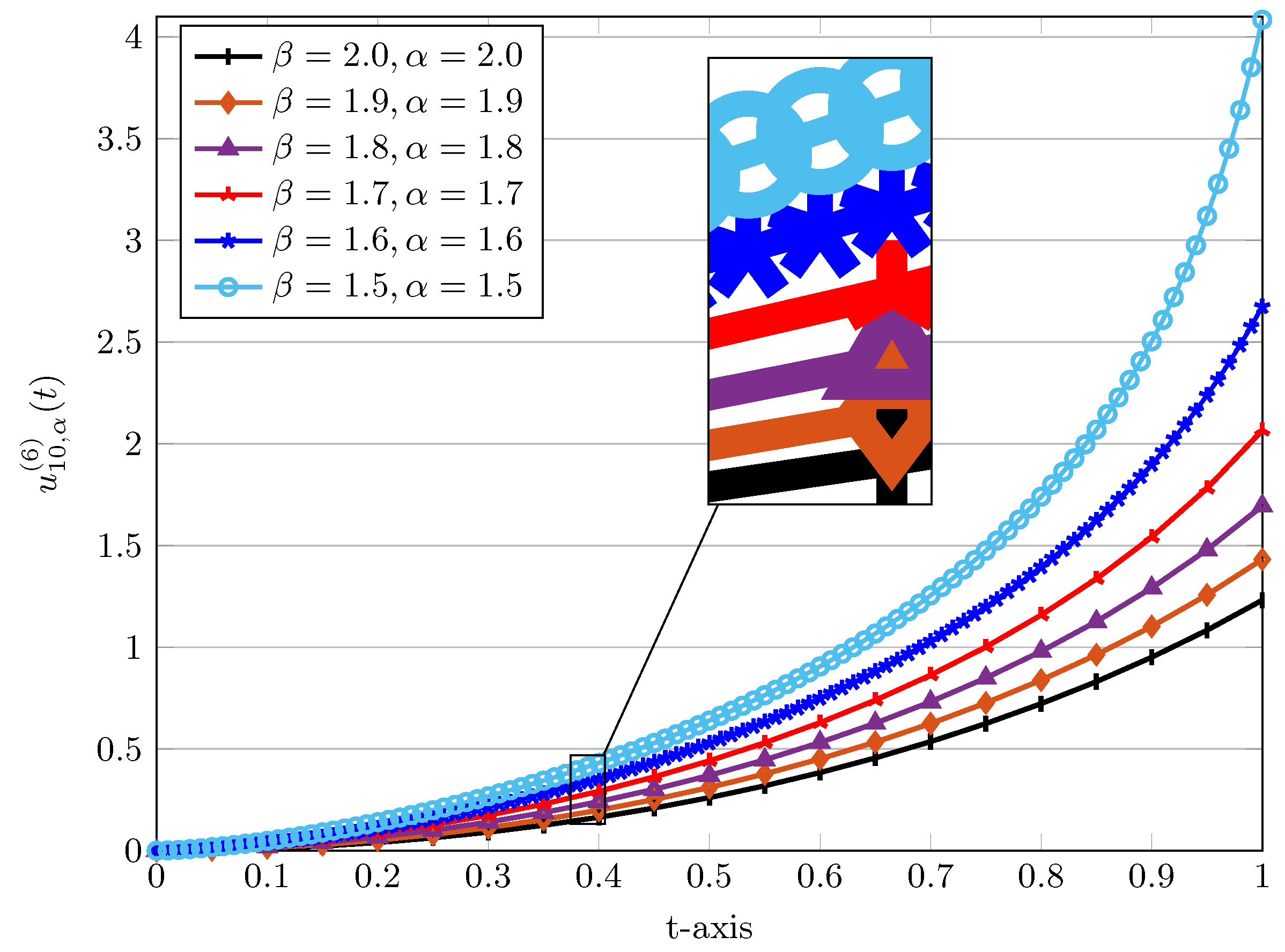
From Table 1 and Table 2, one observes that our result obtained by the presented linearized Bessel-QLM method has a lower magnitude of errors compared to the TWM, the RKM, and LSM. We now return to the fractional-order case and consider different values of β = 2 , 1.9 , , 1.5 . Furthermore, for each value of β , we utilized α = β in the computations. Figure 2 visualizes these approximative solutions with M = 10 and s = 5 . The numerical results obtained using α equal to β in Bessel-QLM are reported in Table 3. Comparisons between numerical solutions obtained via Bessel-QLM and the RKM are further reported in Table 3.
In order to show that our results presented in Table 3 are more accurate than the RKM, we further compared our results with that of the fractional differential transform method (FDTM) [20]. The three-term analytical solution obtained via FDTM is given by [20]:
u F D T M , β ( t ) = 2 c 1 t β + 4 c 2 t 2 β + ( 8 c 3 + 4 c 1 2 c 3 c 2 ) t 3 β + ,
where c j = 1 Γ ( 1 + j β ) for j = 1 , 2 , 3 . The numerical solutions for diverse β = 1.5 , 1.6 , 1.7 , 1.8 , and β = 1.9 evaluated at t = 0.1 are compared in Table 4.
Example 2.
In the second example, let us consider the boundary value Bratu equation:
LC D t β u ( t ) + λ e u ( t ) = 0 , 1 < β 2 , 0 < t < 1 .
The boundary conditions are u ( 0 ) = 0 , u ( 1 ) = 0 . If β = 2 , the exact solution is obtained as:
u ( t ) = 2 ln cosh ( t 0.5 ) ξ 2 + 2 ln cosh ξ 4 ,
where ξ satisfies ξ = 2 λ cosh ξ 4 . In particular, for λ = π 2 , two exact solutions are given by u ( t ) = ln ( 1 ± cos ( π 2 + π t ) ) .
Let us first consider λ = π 2 . In this case, we first consider β = 2 and α = 1 . Using both direct and Bessel-QLM approaches, the following approximations with M = 8 are obtained on t [ 0 , 1 ] :
u 8 , 2 ( t ) = 0.675328868 t 8 2.701317397 t 7 + 5.376111992 t 6 6.67372118 t 5 + 6.402894608 t 4 4.834459802 t 3 + 4.894176844 t 2 3.13901386 t + 1.13899 × 10 13 .
u 8 , 2 ( 6 ) ( t ) = 0.675332096 t 8 2.70132839 t 7 + 5.37612749 t 6 6.67373314 t 5 + 6.40290002 t 4 4.83446126 t 3 + 4.89417706 t 2 3.13901389 t 9.15461 × 10 108 .
Note, the initial guess used in the iterative Bessel-QLM is u 0 ( t ) = t 2 t . The above computed solutions are very close together and are convergent to the exact solution u ( t ) = ln ( 1 + sin ( π t ) ) . The results are depicted in Figure 3. The difference between the approximated solutions and the corresponding exact solutions are also plotted on semilogarithmic scale in Figure 3. In addition to M = 8 , we used M = 12 , 16 , and M = 20 in the Bessel-QLM. The behavior of absolute errors shows the exponential decays with respect to increasing M in the Bessel-QLM algorithm.
We further investigated the convergence and accuracy of the presented Bessel-QLM for β = 2 by computing the values of absolute errors on [ 0 , 1 ] via (45). In Table 5, the numerical results at some points t [ 0 , 1 ] with M = 15 , as well as M = 30 are shown. The results of the TWM [36] are also reported in Table 5 for comparison purposes. Here, M 1 is the order of Taylor polynomials, and the bold numbers in Table 5 represent the correct digits obtained by Bessel-QLM.
The behavior of the numerical solutions based on Bessel-QLM using integer order β = 2 and fractional orders β = 1.9 , 1.8 , , 1.5 was investigated in the next simulations; see Figure 4. The results corresponding to β = 1.9 , 1.7 , 1.5 are provided in Table 6, which were computed at some points t [ 0 , 1 ] . We ran Bessel-QLM when M = 15 , α = 1 , and s = 5 . It can be observed from Figure 4 that the approximated solutions of fractional-order boundary value problem (4) for various values of 1 < β < 2 tend continuously to the numerical and exact solutions when β = 2 .
For the second example, we finally considered λ = 1 , 2 , and λ = 3 . In these cases, we considered β = 1.8 and α = 1 . Utilizing M = 20 , we compared our numerical solutions with the outcomes of the Legendre reproducing kernel method (L-RKM) [21] using the parameters m = 20 and n = 30 . The results are presented in Table 7.

6.2. Model Problem (b)

For the collocation points (19), we take ϵ = 0.1 .
Example 3.
For the second problem type, the following initial value Lane–Emden equation is considered:
LC D t β u ( t ) + 2 t β 1 u ( t ) + e η u ( t ) = 0 , 1 < β 2 , 0 < t < 1 ,
with initial conditions u ( 0 ) = 0 , u ( 0 ) = 0 . For η = ± 1 and β = 2 , the series solutions obtained via the Adomian decompositions method (ADM) [9] are calculated as follows:
u A D M ± ( t ) t 2 6 ± t 4 5 · 4 ! 8 t 6 21 · 6 ! ± 122 t 8 81 · 8 ! 61 · 67 t 10 495 · 10 ! ± .
We use them for comparisons, below.
We begin with β = 2 and α = 1 . Using M = 8 , the resulting approximate solutions obtained via direct Bessel collocation take the following forms on t [ 0 , 1 ] for η = ± 1 respectively as:
u 8 , 1 + ( t ) = 1.1891 × 10 17 1.3793 × 10 17 t 0.1666676405 t 2 + 7.65349 × 10 6 t 3 + 0.008303949361 t 4 + 6.63278 × 10 5 t 5 0.0006203345731 t 6 + 7.33078 × 10 5 t 7 + 9.04876 × 10 6 t 8 ,
u 8 , 1 ( t ) = 1.9683 × 10 18 8.7921 × 10 18 t 0.1666689616 t 2 + 1.76893 × 10 5 t 3 0.008399660792 t 4 + 1.44771 × 10 4 t 5 0.0007189563923 t 6 + 1.42282 × 10 4 t 7 8.66915 × 10 5 t 8 ,
which are very close to the solutions u A D M ± ( t ) . The corresponding numerical approximations by the Bessel-QLM approach with s = 5 and u 0 ( t ) = t 2 are:
u 8 , 1 ( 6 ) , + ( t ) = 8.7435 × 10 110 + 1.7010 × 10 109 t 0.1666676398 t 2 + 7.64838 × 10 6 t 3 + 0.008303967598 t 4 + 6.62906 × 10 5 t 5 0.0006202902396 t 6 + 7.32790 × 10 5 t 7 + 9.05666 × 10 6 t 8 ,
u 8 , 1 ( 6 ) , ( t ) = 4.16087 × 10 110 2.0526 × 10 109 t 0.1666679598 t 2 + 1.00426 × 10 5 t 3 0.008371154811 t 4 + 8.32129 × 10 5 t 5 0.0006395436956 t 6 + 8.42614 × 10 5 t 7 6.74028 × 10 5 t 8 .
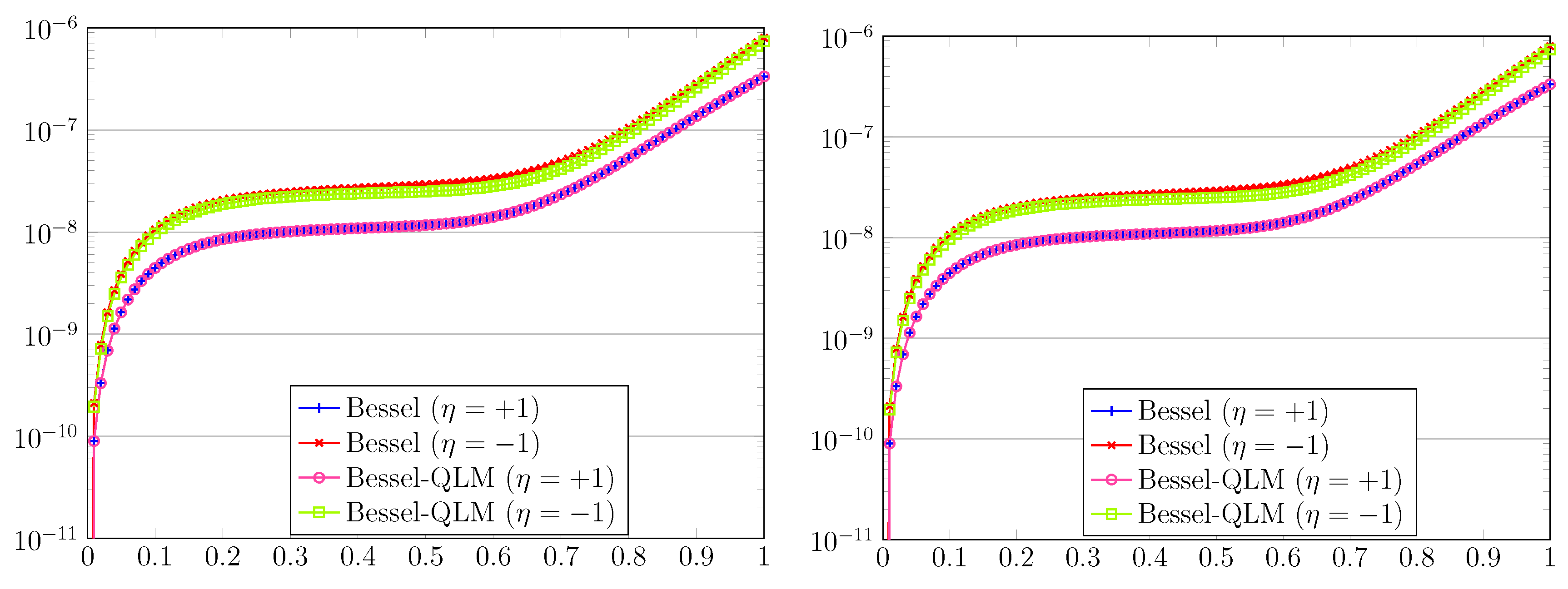
A comparison between the above solutions indicates that the approximate solutions obtained via the Bessel-QLM are also accurate and are close to those obtained by the ADM. To see the discrepancy between solutions more visibly, we plot the graphs of errors | u A D M ± ( t ) u M , α ( t ) | and | u A D M ± ( t ) u M , α ( s + 1 ) ( t ) | for t [ 0 , 1 ] in Figure 5. Moreover, the estimated residual error functions obtained via (41) and (42) are also visualized in Figure 5.
Let us show further the benefits of our presented Bessel-QLM for β = 2 . In this respect, we compared our numerical results for Example 3 in terms of the accuracy and magnitude of errors computed at some t in [ 0 , 1 ] . The following numerical models were used: the ADM [9], the Lagrange operational matrix methods (LOMMs) [34], and the Jacobi operational matrix methods (JOMMs) [37]. The numerical results obtained via (28) using M = 9 , η = + 1 , and α = 1 , 2 are shown in Table 8. Furthermore, Table 8 reports the comparison of residual error functions achieved via (42) with M = 12 , η = ± 1 , and α = 1 , 2 . By looking at the results presented in Table 8 and Table 9, we find that our proposed approach gives clearly more accurate outcomes in comparison with the ADM, LOMMs, and JOMMs.
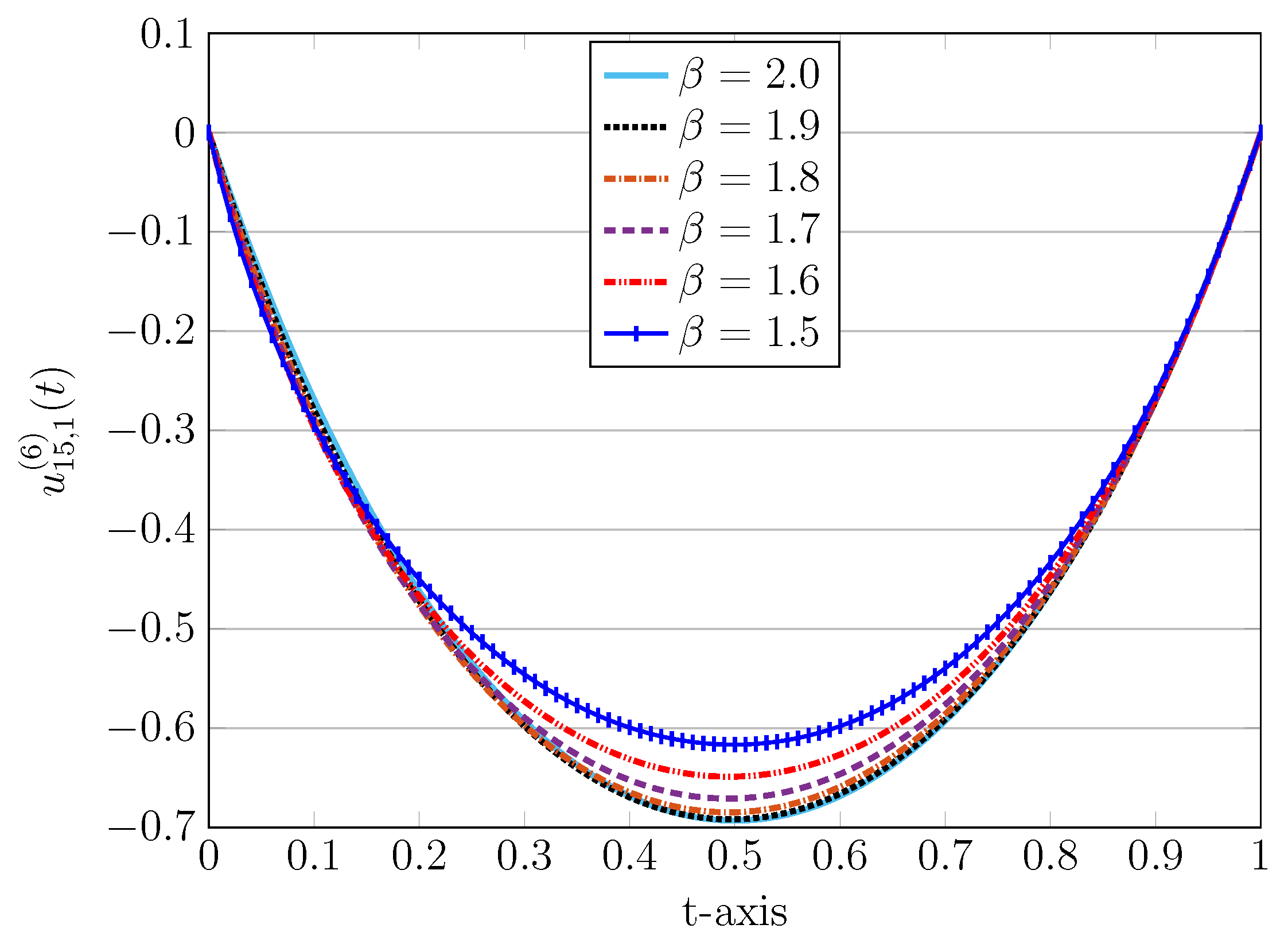
We next utilized the Bessel-QLM to acquire the approximate solutions of this problem when β is a fractional number. In Figure 6, the graphs of numerical solutions corresponding to β = 1.9 , 1.8 , , 1.5 are depicted. Besides, when β = 2 , we plot the numerical solution and its corresponding approximation obtained via AMD [9]. Both cases η = ± 1 in Model Problem 3 were considered with M = 10 and α = 1 . Moreover, numerical results with M = 10 and β equal to α = 1.9 , 1.7 , 1.5 at some points t [ 0 , 1 ] are tabulated in Table 10. For η = + 1 , a comparison with the outcomes of the method based on the homotopy perturbation method and the Adomian decomposition method (HPMADM) [25] are presented in Table 10. Indeed, the following analytical solution via HPMADM was obtained in [25]:
u H , β ( t ) = t β Γ ( 1 + β ) + 2 β + c 1 Γ ( 1 + β ) t 2 β Γ ( 1 + 2 β ) + 4 β Γ ( 1 + β ) + ( 1 2 c 1 2 + c 2 ) Γ ( 1 + 2 β ) t 3 β Γ ( 1 + 3 β ) + 6 β Γ ( 1 + 2 β ) + ,
where c 1 = 1 Γ ( 1 + β ) + 2 β and c 2 = c 1 Γ ( 1 + β ) Γ ( 1 + 2 β ) + 4 β Γ ( 1 + β ) . Note that for β = 2 , the former solution coincides with that of u A D M + ( t ) obtained in [9].
Example 4.
In the fourth example, the subsequent boundary value Lane–Emden problem is considered [38]:
LC D t β u ( t ) + 1 t β 1 u ( t ) + e u ( t ) = 0 , 1 < β 2 , 0 < t < 1 .
The supplemented boundary conditions were u ( 0 ) = 0 , u ( 1 ) = 0 . The exact solution of this test example for β = 2 is given by u ( t ) = 2 ln C + 1 C t 2 + 1 , where C = 3 2 2 .
As before, we first considered β = 2 and α = 1 . The initial guess was taken as u 0 ( t ) = 0 . Utilizing the Bessel-QLM with M = 10 and s = 5 , the approximate solution u M , α ( s + 1 ) ( t ) for 0 t 1 takes the form:
u 10 , 1 ( 6 ) ( t ) = 0.3166943535 + 8.5159 × 10 109 t 0.343145025 t 2 6.7576 × 10 6 t 3 + 0.02947158853 t 4 1.1225 × 10 4 t 5 0.003118318089 t 6 3.7858 × 10 4 t 7 + 8.2207 × 10 4 t 8 2.5302 × 10 4 t 9 + 2.5935 × 10 5 t 10 .
The approximative solution u M , α ( t ) obtained via the direct approach is:
u 10 , 1 ( t ) = 0.3166945657 2.3377 × 10 16 t 0.3431475933 t 2 1.5154 × 10 5 t 3 + 0.02936926925 t 4 + 1.8821 × 10 4 t 5 0.003698759586 t 6 + 3.6075 × 10 4 t 7 + 2.2245 × 10 4 t 8 + 2.8746 × 10 5 t 9 3.2641 × 10 5 t 10 ,
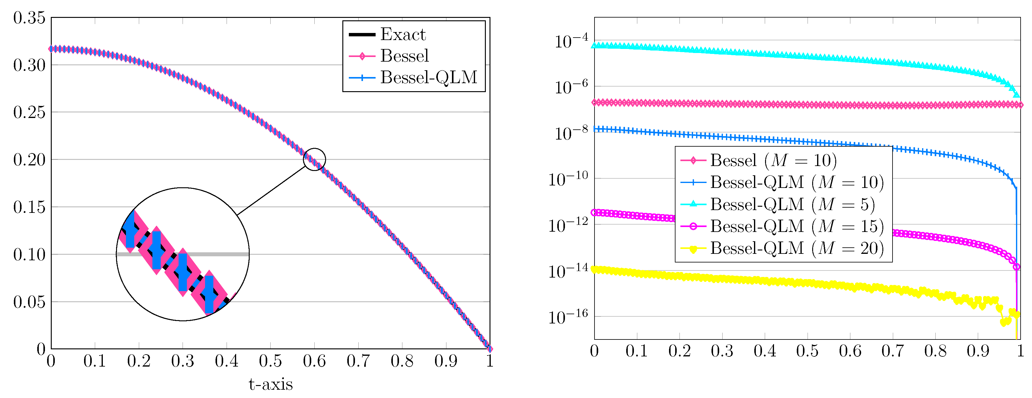
which clearly indicates that both solutions coincide. In order to show that the two obtained solutions are very near the exact solution, we plot their graphs in Figure 7. The corresponding absolute errors can be seen on the right plot. Additionally, we depict the absolute errors in the Bessel-QLM using M = 5 , 15 and M = 20 to indicate that the proposed method has an appropriate convergence rate.
For β = 2 , α = 1 , we further compared our numerical results with regard to the achieved absolute errors (45) in Bessel-QLM. The selected method for comparison is the Laguerre wavelets operational matrix method (LWOMM) [38]. The results using M = 10 and M = 15 are presented in Table 11. As clearly seen, our numerical results are comparably more accurate while needing less computational effort. Additionally, the graph of u 10 , 1 ( 6 ) ( t ) for various values of β = 2 , 1.9 , , 1.5 with M = 10 for Example 4 is visualized in Figure 8. Note that for β = 2 , we also plot the corresponding exact solution, which is known. Finally, in Table 12, the values of the numerical solutions for various fractional values of β = α = 1.9 , 1.7 , 1.5 at different points t [ 0 , 1 ] are reported.
Now, we calculate the weighted L 2 error norms of the approximated solutions using the Bessel-QLM as stated in Theorem 1 and used in Theorem 2 for Examples 1–4. Thus, we compute:
L M , α : = 0 1 [ E M , α ( s + 1 ) ( t ) ] 2 w ( t ) d t , E M , α ( s + 1 ) ( t ) = | u M , α ( s + 1 ) ( t ) u ( t ) | .
When the exact solution is not available, we replace E M , α ( s + 1 ) ( t ) with the residual error functions defined in (41) or (42). To confirm our theoretical analysis, the estimated order of convergence is further computed through defining:
EOC : = L M , α L 2 M , α ln 2 .
The results for β = 2 , α = 1 , and various values of M = 2 j , j = 0 , 1 , 2 , 3 , 4 are presented in Table 13. It should be emphasized that for Examples 1 and 4, we calculate the norms of the corresponding residuals rather than the norms of E M , α ( s + 1 ) ( t ) . It can be obviously seen that the exponential convergence rate is obtainable if one increases the number of basis functions in Bessel-QLM.
Finally, we considered an example for the model problem (1) with nonzero initial conditions. This example was taken from [25], which also showed the advantages of using fractional-order basis functions over the integer-order ones with α = 1 .
Example 5.
The last example is devoted to the following fractional Lane–Emden model problem:
LC D t β u ( t ) + 2 t β 1 u ( t ) = u ( t ) , 1 < β 2 , 0 < t < 1 .
where is submissive to the initial conditions u ( 0 ) = 1 , u ( 0 ) = 0 . For β = 2 , the exact solution is obtained as u ( t ) = sin t t .
We first set β = 2 . Utilizing M = 5 and α = 1 , the following approximation is obtained via Bessel-QLM (with s = 5 ) as
u 5 , 1 ( 6 ) ( t ) = 1.0 + 6.6531 × 10 111 t 0.1665796697 t 2 3.7424 × 10 4 t 3 + 9.0154 × 10 3 t 4 5.8780 × 10 4 t 5 .
More accurate results are obtained using the same M = 5 , but with α = 2 . The approximate solution is:
u 5 , 2 ( 6 ) ( t ) = 1.0 0.1666666646 t 2 + 0.008333320007 t 4 1.9837 × 10 4 t 6 + 2.7037 × 10 6 t 8 .
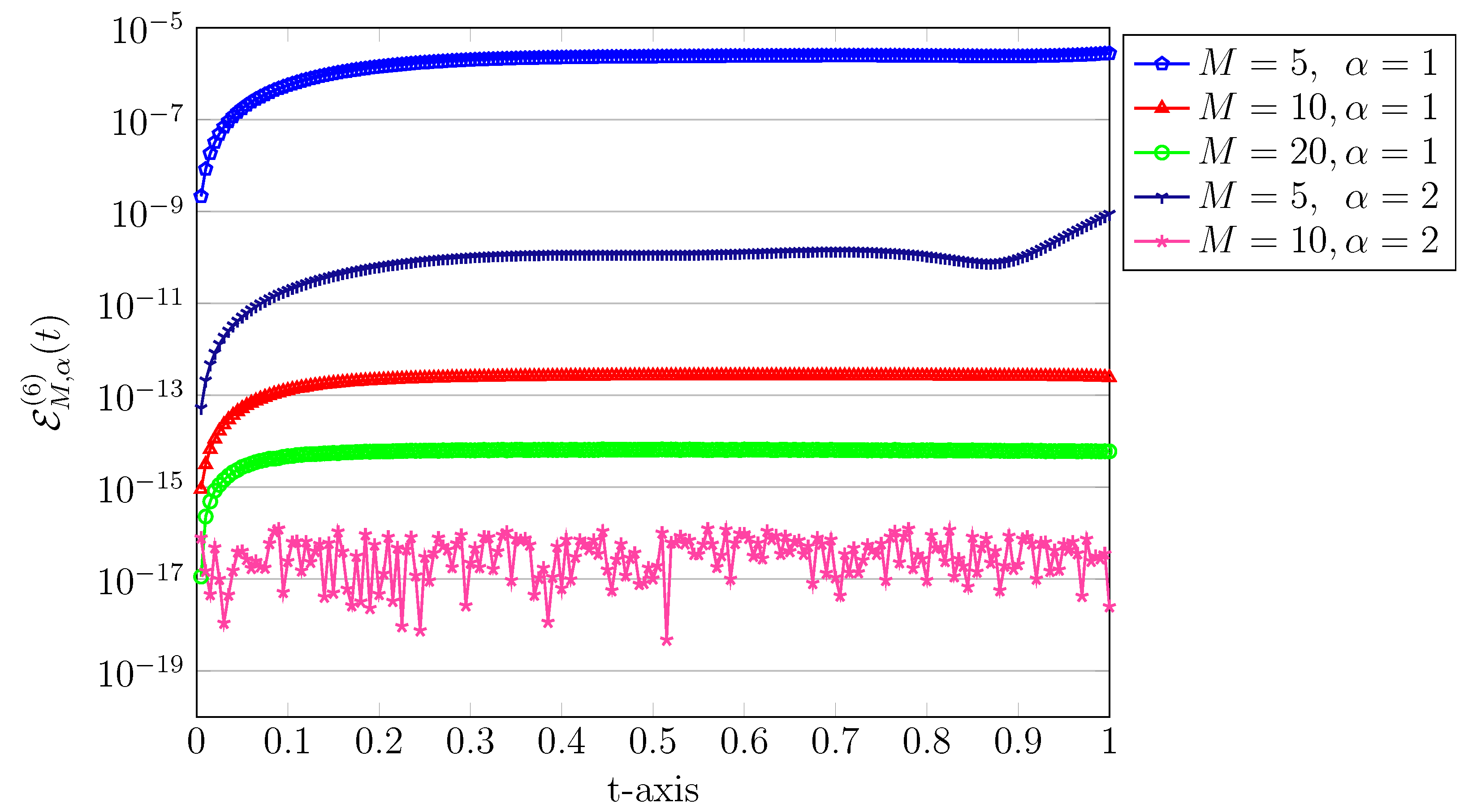
In order to highlight better the difference between the above approximate solutions, we plot the graphs of the corresponding absolute errors E M , α ( s + 1 ) ( t ) in Figure 9. In addition to M = 5 , the results for M = 10 , 20 are also depicted in Figure 9.
We now turn to the fractional-order cases 1 < β < 2 . In these cases, we utilize the technique HPMADM proposed in [25] to acquire the exact analytical solution with three terms as:
u H , β ( t ) = 1 c 1 t β + c 1 Γ ( 1 + β ) Γ ( 1 + 2 β ) + 4 β Γ ( 1 + β ) t 2 β + ,
where c 1 = 1 Γ ( 1 + β ) + 2 β . We exploited this solution as a reference below. To proceed, we considered different values of β = 1.1 , 1.3 , 1.5 , 1.7 , and β = 1.9 . In all cases, we set α equal to β . By using M = 10 , the numerical solutions along with the related solutions u H , β ( t ) are depicted in Figure 10. Note, we also plot the numerical and exact solutions for β = 2 to indicate that other solutions for 1 < β < 2 tend continuously to this case as β approaches two. Obviously, a good agreement between our solutions with that of HPMADM is visible in particular in the first half of the domain.
Next, we show that our numerical solutions u 10 , α ( 6 ) ( t ) with ten terms in Bessel-QLM are more accurate than the corresponding three-term solutions u H , β ( t ) obtained via HPMADM. For this purpose, we compute the residual error function related to this model problem as:
R M , α ( s + 1 ) ( t ) = LC D t β u M , α ( s + 1 ) ( t ) + 2 t β 1 ( u M , α ( s + 1 ) ( t ) ) + u M , α ( s + 1 ) ( t ) 0 , t [ 0 , 1 ] ,
The results of error functions using M = 10 and diverse values of β = 1.1 , 1.3 , 1.5 , 1.7 , 1.9, 2 equal to α are presented in Table 14.
The exponential order of convergence for Example 5 was examined in the last experiments. As for Examples 1–4, we calculated the weighted L 2 error norms and the related EOCs in Bessel-QLM for Example 5. The results for β , α = 1.01 , 1.25 , 1.50 , 1.75 , 1.99 and different values of M = 1 , 2 , 4 , 8 are summarized in Table 15.

7. Conclusions

A novel matrix method in terms of generalized Bessel functions, which is based on some suitable collocation points, was developed for the approximate solutions of integer- and fractional-order nonlinear Bratu and Lane–Emden-type differential equations. By applying the direct Bessel collocation method, the governing equations are transformed into a nonlinear fundamental matrix equation, which may be solved ineffectively for a large number of Bessel functions. To get rid of the nonlinearity, a variant of this algorithm based on the quasilinearization technique, i.e., the Bessel-QLM, was then presented to solve the Bratu and Lane–Emden of arbitrary order with various initial and boundary conditions efficiently. The error and convergence analysis of the Bessel-QLM was also established. Several numerical test examples were presented to describe the applicability and validity of the combined collocation and quasilinearization techniques, and comparisons were made with available well-known numerical model results. On the basis of the numerical calculation together with their comparative results provided in the last part, one can conclude that the integer- and noninteger-order Bratu and the singular Lane–Emden equations can be solved effectively by using the generalized Bessel-QLM. A main advantage of the presented approach is that the solutions of these model problems are obtained very easily ad straightforwardly by means of today’s modern mathematical software.

Author Contributions

Conceptualization, M.I. and H.M.S.; funding acquisition, H.M.S.; investigation, M.I. and H.M.S.; methodology, M.I.; software, M.I.; supervision, H.M.S.; validation, H.M.S.; visualization, M.I.; writing—original draft, M.I.; writing—review and editing, M.I. and H.M.S. All authors have read and agreed to the published version of the manuscript.

Funding

This research received no external funding.

Institutional Review Board Statement

Not applicable.

Informed Consent Statement

Not applicable.

Data Availability Statement

Not applicable.

Conflicts of Interest

The authors declare no conflict of interest.

References

  1. Srivastava, H.M. Some parametric and argument variations of the operators of fractional calculus and related special functions and integral transformations. J. Nonlinear Convex Anal. 2021, 22, 1501–1520. [Google Scholar]
  2. Srivastava, H.M. An introductory overview of fractional-calculus operators based upon the Fox-Wright and related higher transcendental functions. J. Adv. Eng. Comput. 2021, 5, 135–166. [Google Scholar]
  3. Podlubny, I. Fractional Differential Equations; Academic Press: New York, NY, USA, 1999. [Google Scholar]
  4. Wan, Y.; Guo, Q.; Pan, N. Thermo-electro-hydrodynamic model for electrospinning process. Int. J. Nonlinear Sci. Numer. Simul. 2004, 5, 5–8. [Google Scholar] [CrossRef]
  5. Zahoor Raja, M.A.; Samar, R.; Alaidarous, E.S.; Shivanian, E. Bio-inspired computing platform for reliable solution of Bratu-type equations arising in the modeling of electrically conducting solids. Appl. Math. Model. 2016, 40, 5964–5977. [Google Scholar] [CrossRef]
  6. Chandrasekhar, S. An Introduction to the Study of Stellar Structure; Dover Publications: New York, NY, USA, 1967. [Google Scholar]
  7. Davis, H.T. Introduction to Nonlinear Differential and Integral Equations; Dover: New York, NY, USA, 1962. [Google Scholar]
  8. Kilbas, A.A.; Srivastava, H.M.; Trujillo, J.J. Theory and Applications of Fractional Differential Equations; North-Holland Mathematical Studies; Elsevier (North-Holland) Science Publishers: Amsterdam, The Netherlands; London, UK; New York, NY, USA, 2006. [Google Scholar]
  9. Wazwaz, A.M. A new algorithm for solving differential equations of Lane–Emden-type. Appl. Math. Comput. 2001, 118, 287–310. [Google Scholar] [CrossRef]
  10. Babolian, E.; Javadi, S.; Moradia, E. RKM for solving Bratu-type differential equations of fractional order. Math. Methods Appl. Sci. 2016, 39, 1548–1557. [Google Scholar] [CrossRef]
  11. Izadi, M.; Negar, M.R. Local discontinuous Galerkin approximations to fractional Bagley-Torvik equation. Math. Methods Appl. Sci. 2020, 43, 4798–4813. [Google Scholar] [CrossRef]
  12. Izadi, M.; Afshar, M. Solving the Basset equation via Chebyshev collocation and LDG methods. J. Math. Model. 2021, 9, 61–79. [Google Scholar]
  13. Diethelm, K.; Ford, N.J.; Freed, A.D. A predictor-corrector approach for the numerical solution of fractional differential equations. Nonlinear Dyn. 2002, 29, 3–22. [Google Scholar] [CrossRef]
  14. Roul, P.; Prasad Goura, V.M.K. A Bessel collocation method for solving Bratu’s problem. J. Math. Chem. 2020, 58, 1601–1614. [Google Scholar] [CrossRef]
  15. Yüzbaşı, Ş.; Yildirim, G. A Laguerre approach for solving of the systems of linear differential equations and residual improvement. Comput. Methods Differ. Equ. 2021, 9, 553–576. [Google Scholar]
  16. Nouri, K.; Torkzadeh, L.; Mohammadian, S. Hybrid Legendre functions to solve differential equations with fractional derivatives. Math. Sci. 2018, 12, 129–136. [Google Scholar] [CrossRef] [Green Version]
  17. Adel, W.; Sabir, Z. Solving a new design of nonlinear second-order Lane–Emden pantograph delay differential model via Bernoulli collocation method. Eur. Phys. J. Plus 2020, 135, 427. [Google Scholar] [CrossRef]
  18. Izadi, M.; Srivastava, H.M. A novel matrix technique for multi-order pantograph differential equations of fractional order. Proc. R. Soc. Lond. Ser. A Math. Phys. Eng. Sci. 2021, 477, 2021031. [Google Scholar]
  19. Wang, H.-H.; Hu, Y.; Wang, K.-L. The Adomian decomposition method and the fractional complex transform for fractional Bratu-type equation. Therm. Sci. 2017, 21, 1713–1717. [Google Scholar] [CrossRef]
  20. Demir, D.D.; Zeybek, A. The numerical solution of fractional Bratu-type differential equations. In ITM Web of Conferences; EDP Sciences: Les Ulis, France, 2017; Volume 13, p. 01008. [Google Scholar]
  21. Sakar, M.G.; Saldlr, O.; Akgü, A. Numerical solution of fractional Bratu type equations with Legendre reproducing kernel method. Int. J. Appl. Comput. Math. 2018, 4, 126. [Google Scholar] [CrossRef] [Green Version]
  22. Dubey, V.P.; Kumar, R.; Kumar, D.A. Analytical study of fractional Bratu-type equation arising in electro-spun organic nanofibers elaboration. Phyica A 2019, 521, 762–772. [Google Scholar] [CrossRef]
  23. Singh, H.; Ghassabzadeh, F.A.; Tohidi, E.; Cattani, C. Legendre spectral method for the fractional Bratu problem. Math. Methods Appl. Sci. 2020, 43, 5941–5952. [Google Scholar] [CrossRef]
  24. Alchikh, R.; Khuri, S.A. On the solutions of the fractional Bratu’s problem. J. Interdiscip. Math. 2020, 23, 1093–1107. [Google Scholar] [CrossRef]
  25. Wei, C.-F. Application of the homotopy perturbation method for solving fractional Lane–Emden-type equation. Therm. Sci. 2019, 23, 2237–2244. [Google Scholar] [CrossRef]
  26. Izadi, M. A discontinuous finite element approximation to singular Lane–Emden-type equations. Appl. Math. Comput. 2021, 401, 126115. [Google Scholar]
  27. Kazemi Nasab, A.; Pashazadeh Atabakan, Z.; Ismail, A.I.; Ibrahim, R.W. A numerical method for solving singular fractional Lane–Emden-type equations. J. King Saud Univ. Sci. 2018, 30, 120–130. [Google Scholar] [CrossRef]
  28. Sahu, P.K.; Mallick, B. Approximate solution of fractional order Lane–Emden-type differential equation by orthonormal Bernoulli’s polynomials. Int. J. Appl. Comput. Math. 2019, 5, 89. [Google Scholar] [CrossRef]
  29. Izadi, M.; Cattani, C. Generalized Bessel polynomial for multi-order fractional differential equations. Symmetry 2020, 12, 1260. [Google Scholar] [CrossRef]
  30. Izadi, M.; Srivastava, H.M. An efficient approximation technique applied to a non-linear Lane–Emden pantograph delay differential model. Appl. Math. Comput. 2021, 401, 126123. [Google Scholar]
  31. Krall, H.L.; Frink, O. A new class of orthogonal polynomials: The Bessel polynomials. Trans. Amer. Math. Soc. 1949, 65, 100–115. [Google Scholar] [CrossRef]
  32. Bellman, R.E.; Kalaba, R.E. Quasilinearization and Nonlinear Boundary-Value Problems; Elsevier Publishing Company: New York, NY, USA, 1965. [Google Scholar]
  33. Saeed, U.; Rehman, M. Haar wavelet-quasilinearization technique for fractional nonlinear differential equations. Appl. Math. Comput. 2013, 220, 630–648. [Google Scholar] [CrossRef]
  34. Devi, N.; Maurya, R.K.; Patel, V.K.; Singh, V.K. Lagrange operational matrix methods to Lane–Emden, Riccati’s and Bessel’s equations. Int. J. Appl. Comput. Math. 2019, 5, 79. [Google Scholar] [CrossRef]
  35. Izadi, M. An approximation technique for first Painlevé equation. TWMS J. App. Eng. Math. 2021, 11, 739–750. [Google Scholar]
  36. Keshavarz, E.; Ordokhani, Y.; Razzaghi, M. The Taylor wavelets method for solving the initial and boundary value problems of Bratu-type equations. Appl. Numer. Math. 2018, 125, 205–216. [Google Scholar] [CrossRef]
  37. Singh, H.; Srivastava, H.M.; Kumar, D. A reliable algorithm for the approximate solution of the nonlinear Lane–Emden-type equations arising in astrophysics. Numer. Methods Partial Differ. Equ. 2018, 34, 1524–1555. [Google Scholar] [CrossRef]
  38. Zhou, F.; Xu, X. Numerical solutions for the linear and nonlinear singular boundary value problems using Laguerre wavelets. Adv. Differ. Equ. 2016, 2016, 17. [Google Scholar] [CrossRef]
Figure 1. The graphs of approximated and exact solutions (left) and the related absolute errors (right) for β = 2 , α = 1 , M = 10 , and s = 5 in Example 1.
Fractalfract 05 00179 g001
Figure 2. The approximated Bessel-QLM series solutions for Example 1 using various β , α = 1.5 , 1.6, , 2 for M = 10 , s = 5 .
Fractalfract 05 00179 g002
Figure 3. The graphs of numerical and exact solutions for M = 8 (left) and the resulting absolute errors for M = 8 , 12 , 16 , 20 (right) for β = 2 , α = 1 , λ = π 2 , and s = 5 in Example 2.
Fractalfract 05 00179 g003
Figure 4. Numerical approximations in Bessel-QLM for various β = 2 , 1.9 , , 1.5 , α = 1 , λ = π 2 , and M = 15 in Example 2.
Fractalfract 05 00179 g004
Figure 5. The graphs of of errors (left) and the resulting residual errors (right) for β = 2 , α = 1 , M = 8 , and s = 5 in Example 3.
Fractalfract 05 00179 g005
Figure 6. Approximated solutions with η = + 1 (left) and η = 1 (right) in Bessel-QLM for M = 10 , α = 1 , s = 5 , and various β = 1.9 , 1.8 , , 1.5 in Example 3.
Fractalfract 05 00179 g006
Figure 7. The graphs of numerical and exact solutions for M = 10 (left) and the resulting absolute errors for M = 5 , 10 , 15 , 20 (right) for β = 2 , α = 1 , and s = 5 in Example 4.
Fractalfract 05 00179 g007
Figure 8. Numerical approximations in Bessel-QLM for various β = 2 , 1.9 , , 1.5 , α = 1 , and M = 10 in Example 4.
Fractalfract 05 00179 g008
Figure 9. Absolute errors in Bessel-QLM for β = 2 , α = 1 , 2 and various M = 5 , 10 , 20 in Example 5.
Fractalfract 05 00179 g009
Figure 10. A comparison of numerical solutions in Bessel-QLM for M = 10 and various 1 < β = α < 2 in Example 5.
Fractalfract 05 00179 g010
Table 1. The comparison of absolute errors using Bessel-QLM in Example 1 for β = 2 , α = 1 , M = 15 , 20 , 25 , 30 , and various t [ 0 , 1 ] .
t E 15 , 1 ( 6 ) ( t ) E 20 , 1 ( 6 ) ( t ) E 25 , 1 ( 6 ) ( t ) u 30 , 1 ( 6 ) ( t ) E 30 , 1 ( 6 ) ( t )
0.1 2.9055 × 10 6 2.5768 × 10 8 1.1549 × 10 10 0.010016711246980 5.0955 × 10 13
0.2 6.7455 × 10 6 5.6983 × 10 8 2.4911 × 10 10 0.040269546105905 1.0880 × 10 12
0.3 1.0727 × 10 5 8.9392 × 10 8 3.8795 × 10 10 0.091383311853805 1.6892 × 10 12
0.4 1.4945 × 10 5 1.2378 × 10 7 5.3536 × 10 10 0.164458038152439 2.3278 × 10 12
0.5 1.9519 × 10 5 1.6110 × 10 7 6.9550 × 10 10 0.261168480890467 3.0217 × 10 12
0.6 2.4605 × 10 5 2.0265 × 10 7 8.7388 × 10 10 0.383930338842670 3.7949 × 10 12
0.7 3.0421 × 10 5 2.5022 × 10 7 1.0782 × 10 9 0.536171515140543 4.6808 × 10 12
0.8 3.7293 × 10 5 3.0647 × 10 7 1.3199 × 10 9 0.722781493628416 5.7288 × 10 12
0.9 4.5727 × 10 5 3.7556 × 10 7 1.6170 × 10 9 0.950884887178646 7.0170 × 10 12
1.0 5.6582 × 10 5 4.6455 × 10 7 1.9996 × 10 9 1.231252940780713 8.6847 × 10 12
Table 2. Comparison of absolute errors in Bessel-QLM for Example 1 using β = α = 2 , M = 5 , 10 , and various t [ 0 , 1 ] .
tBessel-QLM ( α = 2 ) LSM ( n = 9 ) [23]TWM [36]RKM [10]
M = 7 M = 10 Method (a)Method (b) k = 1 , M 1 = 7 n , N = 10
0.1 4.1979 × 10 8 2.0195 × 10 11 1.4169 × 10 5 1.7830 × 10 7 2.69611 × 10 5 1.6674 × 10 5
0.2 1.2167 × 10 7 4.6897 × 10 11 3.2272 × 10 5 4.5055 × 10 7 2.38968 × 10 5 3.1000 × 10 7
0.3 1.8565 × 10 7 7.4344 × 10 11 5.1244 × 10 5 7.1998 × 10 7 1.01329 × 10 5 1.1310 × 10 6
0.4 2.6108 × 10 7 1.0203 × 10 10 7.1441 × 10 5 1.0081 × 10 6 2.12408 × 10 5 2.1200 × 10 6
0.5 3.5454 × 10 7 1.3688 × 10 10 9.2812 × 10 5 1.3195 × 10 6 1.15316 × 10 5 2.9000 × 10 6
0.6 4.1000 × 10 7 1.5831 × 10 10 1.1720 × 10 4 1.6653 × 10 6 1.85136 × 10 5 4.1000 × 10 6
0.7 5.7919 × 10 7 2.6467 × 10 10 1.4496 × 10 4 2.0620 × 10 6 1.15473 × 10 5 6.5000 × 10 6
0.8 6.8266 × 10 7 1.8342 × 10 10 1.7718 × 10 4 2.2525 × 10 6 2.26494 × 10 5 7.5000 × 10 6
0.9 3.0427 × 10 7 6.5824 × 10 09 2.1791 × 10 4 3.1212 × 10 6 1.13933 × 10 5 3.3500 × 10 5
1.0 3.2344 × 10 5 3.9874 × 10 07 2.6999 × 10 4 3.6311 × 10 6 8.55545 × 10 5 4.3700 × 10 5
Table 3. The comparison of numerical results using Bessel-QLM in Example 1 for M = 10 and various α equal to β = 1.5 , 1.6 , , 1.9 .
tBessel-QLM ( α = β ) RKM ( N = 10 ) [10]
β = 1.5 β = 1.6 β = 1.7 β = 1.8 β = 1.9 β = 1.5 β = 1.6 β = 1.7 β = 1.8 β = 1.9
0.1 0.048353 0.035473 0.025993 0.018983 0.013814 0.047581 0.035141 0.025834 0.018907 0.013779
0.2 0.140366 0.109646 0.085643 0.066769 0.051926 0.14073 0.10984 0.085716 0.066792 0.051932
0.3 0.267489 0.215666 0.174210 0.140695 0.113494 0.26686 0.21547 0.17414 0.14067 0.11349
0.4 0.431675 0.354277 0.292046 0.241173 0.199225 0.43128 0.35420 0.29201 0.24116 0.19922
0.5 0.639964 0.529749 0.441962 0.370277 0.310871 0.63930 0.52957 0.44188 0.37024 0.31086
0.6 0.905877 0.750259 0.629314 0.531789 0.451331 0.90494 0.75001 0.62921 0.53175 0.45132
0.7 1.254902 1.030118 0.863049 0.731769 0.625010 1.2533 1.0297 0.86289 0.73170 0.62499
0.8 1.740090 1.395364 1.158156 0.979794 0.838525 1.7367 1.3946 1.1579 0.97970 0.83849
0.9 2.503677 1.899300 1.541363 1.291531 1.102046 2.4864 1.8967 1.5407 1.2913 1.1020
1.0 4.084549 2.674636 2.066148 1.694499 1.431961 4.0331 2.6677 2.0646 1.6941 1.4318
Table 4. The comparison of the numerical results using Bessel-QLM in Example 1 for M = 10 and various α equal to β = 1.5 , 1.6 , , 1.9 at t = 0.1 .
β Bessel-QLM ( α = β ) RKM ( N = 10 ) [10]FDTM ( N = 5 ) [20]
1.9 0.013814 1.3082 × 10 2 1.3814 × 10 2
1.8 0.018983 1.7221 × 10 2 1.8983 × 10 2
1.7 0.025993 2.2504 × 10 2 2.5993 × 10 2
1.6 0.035473 2.9221 × 10 2 3.5472 × 10 2
1.5 0.048353 3.7921 × 10 2 4.8260 × 10 2
Table 5. The comparison of the numerical results using Bessel-QLM in Example 2 with M = 15 , 30 , s = 5 , and β = 2 , α = 1 , λ = π 2 . Numbers in bold show that the correct digits are obtained by the Bessel-QLM.
tBessel-QLMTWM [36]
U 15 , 1 ( 6 ) ( t ) E 15 , 1 ( 6 ) ( t ) U 30 , 1 ( 6 ) ( t ) E 30 , 1 ( 6 ) ( t ) K = 1 , M 1 = 11
0.1 0.269276 38478 8.4777 × 10 8 0.26927646955 8501 7.6043 × 10 13 5.5884 × 10 8
0.2 0.462340 04975 7.2374 × 10 8 0.462340122126 269 2.0527 × 10 13 7.4576 × 10 8
0.3 0.592783 53642 6.4300 × 10 8 0.59278360071 7044 3.3595 × 10 13 1.3357 × 10 8
0.4 0.66837 096929 5.9790 × 10 8 0.66837102908 2459 8.9516 × 10 13 8.9851 × 10 8
0.5 0.6931471 2222 5.8338 × 10 8 0.6931471805 61445 1.4998 × 10 12 1.4347 × 10 7
0.6 0.66837 096929 5.9790 × 10 8 0.66837102908 3743 2.1792 × 10 12 8.9851 × 10 8
0.7 0.592783 53642 6.4300 × 10 8 0.59278360071 9678 2.9697 × 10 12 1.3357 × 10 8
0.8 0.462340 04975 7.2374 × 10 8 0.4623401221 30420 3.9452 × 10 12 7.4576 × 10 8
0.9 0.269276 384782 8.4777 × 10 8 0.2692764695 64491 5.2293 × 10 12 5.5884 × 10 8
Table 6. Numerical solutions in Bessel-QLM for β = 1.9 , 1.7 , 1.5 in Example 2 for M = 15 , λ = π 2 , and α = 1 .
t β = 1.5 β = 1.7 β = 1.9
0.1 0.294195 0.294574 0.279940
0.2 0.450191 0.475380 0.471703
0.3 0.545938 0.589367 0.598037
0.4 0.599428 0.652366 0.669690
0.5 0.616646 0.670828 0.691846
0.6 0.597974 0.646235 0.666096
0.7 0.539612 0.576307 0.591041
0.8 0.433043 0.454769 0.462076
0.9 0.262495 0.269766 0.270311
Table 7. The comparison of the numerical results using Bessel-QLM in Example 2 with M = 20 , β = 1.8 , λ = 1 , 2 , 3 , and α = 1 .
tBessel-QLML-RKM [21]
λ = 1 λ = 2 λ = 3 λ = 1 λ = 2 λ = 3
0.1 0.056413 0.131924 0.261504 0.056405 0.131612 0.260654
0.2 0.097782 0.231011 0.465679 0.097789 0.230471 0.464144
0.3 0.125742 0.298753 0.608060 0.125778 0.298048 0.606020
0.4 0.141008 0.335519 0.684421 0.141075 0.334699 0.682068
0.5 0.144146 0.342145 0.694381 0.144246 0.341257 0.691916
0.6 0.135734 0.320218 0.642257 0.135863 0.319304 0.639866
0.7 0.116398 0.272047 0.536290 0.116553 0.271144 0.534126
0.8 0.086829 0.200491 0.386913 0.087005 0.199631 0.385081
0.9 0.047770 0.108725 0.204897 0.047961 0.107936 0.203461
Table 8. The comparison of various numerical results with Bessel-QLM for Example 3 for M = 9 , β = 2 , η = + 1 , and α = 1 , 2 .
tBessel-QLM ( η = + 1 )ADM [9]LOMMs ( M = 8 ) [34]
α = 1 α = 2 Scheme-IScheme-II
0.0 0.00000000000 0.00000000000 0.00000000000 2.0346 × 10 10 5.194068 × 10 8
0.1 0.0016658338 0.0016658339 0.0016658339 0.0016658339 0.00166586155
0.2 0.0066533670 0.0066533671 0.0066533671 0.0066533671 0.00665336928
0.5 0.0411539571 0.0411539573 0.0411539568 0.0411539978 0.041154078892
1.0 0.1588276774 0.1588276775 0.1588273537 0.1588370919 0.15883515641
Table 9. The comparison of (residual) error functions using Bessel-QLM in Example 3 with M = 12 , β = 2 and α = 1 , 2 .
tBessel-QLM ( η = + 1 )LOMMs [34]Bessel-QLM ( η = 1 )JOMMs [37]
α = 1 α = 2 Scheme-IScheme-II α = 1 α = 2 η = + 1 η = 1
0.0 0.0000 × 10 + 00 0.0000 × 10 + 00 2.04 × 10 10 5.19 × 10 8 0.0000 × 10 + 00 0.0000 × 10 + 00
0.1 2.7488 × 10 13 3.0158 × 10 22 1.88 × 10 11 5.49 × 10 9 6.8148 × 10 13 5.6265 × 10 16 1.98 × 10 12 4.66 × 10 11
0.2 1.2099 × 10 13 2.8196 × 10 20 2.48 × 10 11 1.73 × 10 8 4.4922 × 10 13 1.1621 × 10 13 1.66 × 10 12 4.02 × 10 11
0.5 4.4965 × 10 15 6.7454 × 10 19 8.70 × 10 8 1.00 × 10 8 2.9402 × 10 9 2.9388 × 10 9 4.64 × 10 10 5.21 × 10 10
1.0 3.6953 × 10 10 9.4919 × 10 14 2.53 × 10 5 2.72 × 10 5 7.4859 × 10 6 7.4850 × 10 6 3.23 × 10 7 7.63 × 10 7
Table 10. Comparison of numerical results in Bessel-QLM for M = 10 and β , α = 1.5 , 1.7 , 19 in Example 3.
t η = + 1 η = 1
Bessel-QLMHPMADM [25]Bessel-QLM
β = 1.5 β = 1.7 β = 1.9 β = 1.5 β = 1.7 β = 1.9 β = 1.5 β = 1.7 β = 1.9
0.1 0.0072824 0.0040292 0.0022355 0.0072824 0.0040292 0.0022355 0.0073264 0.0040412 0.0022388
0.2 0.0204858 0.0130471 0.0083268 0.0204861 0.0130471 0.0083268 0.0208374 0.0131743 0.0083720
0.3 0.0373729 0.0258703 0.0179349 0.0373745 0.0258707 0.0179350 0.0385599 0.0263753 0.0181458
0.4 0.0570711 0.0419374 0.0308502 0.0570774 0.0419393 0.0308506 0.0598865 0.0432809 0.0314797
0.5 0.0790339 0.0608534 0.0468938 0.0790524 0.0608596 0.0468956 0.0845384 0.0637239 0.0483641
0.6 0.1028640 0.0823017 0.0658965 0.1029100 0.0823186 0.0659020 0.1123910 0.0876416 0.0688375
0.7 0.1282516 0.1060115 0.0876918 0.1283516 0.1060515 0.0877059 0.1434138 0.1150420 0.0929785
0.8 0.1549433 0.1317434 0.1121130 0.1551409 0.1318286 0.1121454 0.1776437 0.1459885 0.1209032
0.9 0.1827273 0.1592811 0.1389929 0.1830894 0.1594484 0.1390612 0.2151732 0.1805938 0.1527654
1.0 0.2114227 0.1884270 0.1681640 0.2120480 0.1887346 0.1682981 0.2561452 0.2190184 0.1887588
Table 11. The comparison of numerical solutions using Bessel-QLM with M = 10 , 15 , s = 5 , and β = 2 , α = 1 in Example 3. Numbers in bold show that the correct digits are obtained by the Bessel-QLM.
tBessel-QLMLWOMM [36]
U 10 , 1 ( 6 ) ( t ) E 10 , 1 ( 6 ) ( t ) U 15 , 1 ( 6 ) ( t ) E 15 , 1 ( 6 ) ( t ) K = 3 , M 1 = 7
0.1 0.3132658 39363106 1.1135 × 10 8 0.31326585049 5719 2.3444 × 10 12 1.12567 × 10 11
0.2 0.3030154 14602317 8.2300 × 10 9 0.30301542283 0577 1.7229 × 10 12 1.06202 × 10 11
0.3 0.2860472 58937613 6.3672 × 10 9 0.28604726530 3516 1.3380 × 10 12 9.71828 × 10 12
0.4 0.26253112 2482223 4.9738 × 10 9 0.26253112745 4984 1.0495 × 10 12 8.57608 × 10 12
0.5 0.23269678 0038309 3.8355 × 10 9 0.232696783873 021 8.1360 × 10 13 7.28159 × 10 12
0.6 0.19682680 2831837 2.8611 × 10 9 0.196826805692 342 6.1151 × 10 13 5.78329 × 10 12
0.7 0.15524810 4677472 2.0053 × 10 9 0.155248106682 323 4.3376 × 10 13 4.31280 × 10 12
0.8 0.10832276 2202615 1.2419 × 10 9 0.108322763444 190 2.7506 × 10 13 2.82023 × 10 12
0.9 0.05643860 1915112 5.5412 × 10 10 0.056438602469 104 1.3218 × 10 13 1.33990 × 10 12
Table 12. Numerical solutions in Bessel-QLM for β = 1.9 , 1.7 , 1.5 in Example 4 for M = 10 and α = β .
t β , α = 1.5 β , α = 1.7 β , α = 1.9
0.1 0.4538007 0.3940449 0.3389203
0.2 0.4218743 0.3736066 0.3259879
0.3 0.3816409 0.3447748 0.3056717
0.4 0.3355231 0.3090216 0.2785187
0.5 0.2850841 0.2674419 0.2450333
0.6 0.2314604 0.2209409 0.2057129
0.7 0.1755228 0.1702998 0.1610556
0.8 0.1179554 0.1162043 0.1115587
0.9 0.0593026 0.0592595 0.0577135
Table 13. The weighted L 2 error norms and the related EOCs in Bessel-QLM for Examples 1–4 for β = 2 , α = 1 , and diverse M.
MExample 1Example 2Example 3Example 4
L M , α EOC L M , α EOC L M , α EOC L M , α EOC
1 1.5958 × 10 1 8.5933 × 10 2 8.5933 × 10 1 1.1185 × 10 1
2 3.5672 × 10 2 2.16 7.9098 × 10 3 3.44 7.9098 × 10 3 4.14 1.5476 × 10 2 2.85
4 6.3893 × 10 3 2.48 7.2809 × 10 4 3.44 7.2809 × 10 4 5.94 4.4277 × 10 4 5.13
8 1.3504 × 10 4 5.56 9.6224 × 10 6 6.24 9.6224 × 10 8 12.79 1.4858 × 10 7 11.54
16 4.5362 × 10 8 11.54 2.8868 × 10 8 8.38 2.8868 × 10 11 8.10 6.1046 × 10 11 11.25
Table 14. Residual errors in Bessel-QLM for β = 1.1 , 1.3 , 1.5 , 1.7 , 1.9 in Example 5 for M = 10 and α = β .
t β , α = 1.1 β , α = 1.3 β , α = 1.5 β , α = 1.7 β , α = 1.9 β , α = 2.0
0.1 1.0364 × 10 12 2.0468 × 10 14 3.6172 × 10 16 4.6938 × 10 17 3.4314 × 10 17 2.9295 × 10 19
0.2 1.0825 × 10 11 4.0085 × 10 13 1.1342 × 10 14 4.7141 × 10 16 4.4964 × 10 17 5.6627 × 10 21
0.3 4.2966 × 10 11 2.2006 × 10 12 8.6122 × 10 14 4.7959 × 10 15 8.1274 × 10 16 6.2154 × 10 20
0.4 1.1427 × 10 10 7.3667 × 10 12 3.6292 × 10 13 2.5459 × 10 14 5.4271 × 10 15 2.0139 × 10 19
0.5 2.4401 × 10 10 1.8806 × 10 11 1.1075 × 10 12 9.2932 × 10 14 2.3579 × 10 14 8.3624 × 10 20
0.6 4.5356 × 10 10 4.0444 × 10 11 2.7559 × 10 12 2.6760 × 10 13 7.8496 × 10 14 1.2112 × 10 19
0.7 7.6604 × 10 10 7.7274 × 10 11 5.9566 × 10 12 6.5436 × 10 13 2.1732 × 10 13 4.7674 × 10 19
0.8 1.2062 × 10 9 1.3539 × 10 10 1.1613 × 10 11 1.4194 × 10 12 5.2448 × 10 13 1.2044 × 10 18
0.9 1.8003 × 10 9 2.2204 × 10 10 2.0928 × 10 11 2.8112 × 10 12 1.1418 × 10 12 8.8587 × 10 18
Table 15. The weighted L 2 error norms and the related EOCs in Bessel-QLM for Example 5 for β , α = 1.01 , 1.25 , 1.50 , 1.75 , 1.99 , and diverse M.
M β , α = 1.01 β , α = 1.25 β , α = 1.50 β , α = 1.75 β , α = 1.99
L M , α EOC L M , α EOC L M , α EOC L M , α EOC L M , α EOC
1 1.9232 × 10 1 1.6545 × 10 1 1.4671 × 10 1 1.3314 × 10 1 1.2312 × 10 1
2 1.5972 × 10 2 3.59 1.4895 × 10 2 3.47 1.3526 × 10 2 3.43 1.2065 × 10 2 3.46 1.0666 × 10 2 3.53
4 2.7591 × 10 5 9.17 2.0311 × 10 5 9.52 1.2836 × 10 5 10.04 6.9934 × 10 6 10.75 3.3538 × 10 6 11.64
8 4.1872 × 10 12 22.65 1.2170 × 10 12 23.99 1.9693 × 10 13 25.96 1.8278 × 10 14 28.51 9.7566 × 10 16 31.68
Publisher’s Note: MDPI stays neutral with regard to jurisdictional claims in published maps and institutional affiliations.