Article

Applications of the (G′/G2)-Expansion Method for Solving Certain Nonlinear Conformable Evolution Equations

by
Supaporn Kaewta
1,
Sekson Sirisubtawee
1,2,*,
Sanoe Koonprasert
1,2 and
Surattana Sungnul
1,2
1
Department of Mathematics, Faculty of Applied Science, King Mongkut’s University of Technology North Bangkok, Bangkok 10800, Thailand
2
Centre of Excellence in Mathematics, CHE, Si Ayutthaya Road, Bangkok 10400, Thailand
*
Author to whom correspondence should be addressed.
Fractal Fract. 2021, 5(3), 88; https://doi.org/10.3390/fractalfract5030088
Submission received: 30 June 2021 / Revised: 31 July 2021 / Accepted: 1 August 2021 / Published: 4 August 2021

Abstract

:
The core objective of this article is to generate novel exact traveling wave solutions of two nonlinear conformable evolution equations, namely, the ( 2 + 1 ) -dimensional conformable time integro-differential Sawada–Kotera (SK) equation and the ( 3 + 1 ) -dimensional conformable time modified KdV–Zakharov–Kuznetsov (mKdV–ZK) equation using the ( G / G 2 ) -expansion method. These two equations associate with conformable partial derivatives with respect to time which the former equation is firstly proposed in the form of the conformable integro-differential equation. To the best of the authors’ knowledge, the two equations have not been solved by means of the ( G / G 2 ) -expansion method for their exact solutions. As a result, some exact solutions of the equations expressed in terms of trigonometric, exponential, and rational function solutions are reported here for the first time. Furthermore, graphical representations of some selected solutions, plotted using some specific sets of the parameter values and the fractional orders, reveal certain physical features such as a singular single-soliton solution and a doubly periodic wave solution. These kinds of the solutions are usually discovered in natural phenomena. In particular, the soliton solution, which is a solitary wave whose amplitude, velocity, and shape are conserved after a collision with another soliton for a nondissipative system, arises ubiquitously in fluid mechanics, fiber optics, atomic physics, water waves, and plasmas. The method, along with the help of symbolic software packages, can be efficiently and simply used to solve the proposed problems for trustworthy and accurate exact solutions. Consequently, the method could be employed to determine some new exact solutions for other nonlinear conformable evolution equations.

1. Introduction

Nonlinear evolution equations (NLEEs), which are interpreted as the differential law of the development in time of a system and typically expressed in terms of nonlinear partial differential equations (NPDEs), can be utilized to describe many interesting and sophisticated phenomena in physics, mathematical physics, engineering, and other various scientific fields such as fluid mechanics [1,2], plasma physics [3], quantum mechanics [4], biology [5], nonlinear wave theory [6], and fiber optics [7]. Some applications of NLEEs for natural events are as follows [8,9,10]: The nonlinear Schrödinger’s equation explains the dynamics of propagation for solitons through optical fibers. The Korteweg de Vries (KdV) equation can be used to model the shallow water wave dynamics near ocean shore and beaches. The dynamics of an incompressible viscoelastic Kelvin–Voigt fluid can be described by the Oskolkov equation. In addition, an epidemic model on a network such as the present epidemic of COVID-19 comprising susceptible–infected–recovered equations at the nodes, coupled by diffusion using a graph Laplacian, can be analyzed using a system of NLEEs.
To further elucidate some important behaviors of the phenomena modeled by NLEEs, extracting their exact analytic solutions, in particular, solitary wave solutions, is of great significance. The exploration of exact solutions for NLEEs has become quite prominent due to the recent, considerable advances in computational methods and symbolic software packages. Numerous kinds of exact solutions such as solitons, positons, complexitons, dromions, cuspon, rational, kink, periodic, and quasiperiodic solutions have been obtained via solving integrable NLEEs. In the past couple of decades, many robust, efficient, and powerful methods exist that have been developed for finding exact solutions of NLEEs, including the ( G / G , 1 / G ) -expansion method [11], the enhanced ( G / G ) -expansion method [12], the exp-function method [13], the Jacobi elliptic equation method [14], the generalized Kudryashov’s method [15], the sine-Gordon expansion method [16], the sub-equation method [17], the improved tan ( ϕ / 2 ) -expansion method [18], and the extended direct algebraic method [19,20]. More recently, the ( G / G 2 ) -expansion method [4,21,22,23,24,25,26,27,28,29] has attracted a remarkable amount of attention of many researchers who employed the method to construct exact solutions of certain NPDEs. In 2018, Arshed and Sadia [23] used the ( G / G 2 ) -expansion method to obtain some new traveling wave solutions for the time-fractional Burgers equation, the fractional biological population model, and the space-time fractional Whitham–Broer–Kaup equations. Sirisubtawee and Koonprasert [24] utilized the method to solve the Benny–Luke equation, the equation of nanoionic currents along microtubules, and the generalized Hirota–Satsuma coupled KdV system for their exact solutions including trigonometric, exponential, and rational function solutions. In 2020, the ( G / G 2 ) -expansion approach was employed to construct some novel exact traveling wave solutions of the ( 2 + 1 ) -dimensional Boiti–Leon–Pempinelli system [28]. In 2021, Bilal et al. [29] proposed new exact solutions, which consist of shock, singular, shock-singular, and singular periodic wave solutions obtained by the ( G / G 2 ) -expansion method, to unidirectional Dullin–Gottwald–Holm (DGH) system describing the prorogation of waves in shallow water.
In this article, we will demonstrate the use of the G / G 2 -expansion method to construct explicit exact solutions for the following two interesting problems in mathematical physics:
1. The ( 2 + 1 ) -dimensional conformable time integro-differential Sawada–Kotera (SK) equation can be expressed as
t α u = u x x x x + 5 u u x x + 5 3 u 3 + 5 u x y x 5 x 1 ( u y y ) + 5 u u y + 5 u x x 1 ( u y ) ,
where t α · = α t α · is the conformable partial derivative with respect to t of order α with 0 < α 1 and x 1 · = x · d x . The dependent variable u in the equation is a multivariable function consisting of three independent variables x , y , and t , i.e., u = u ( x , y , t ) . If α = 1 , then Equation (1) reduces into the ( 2 + 1 ) -dimensional integro-differential SK equation [30,31,32,33,34,35,36], which was initially established by Konopelcheno and Dubrovsky [37], using the inverse scattering transform method. The ( 2 + 1 ) -dimensional SK equation has been investigated extensively and intensively in a number of studies in the literature because of its significance and various applications in two-dimensional quantum gravity field theory, conformal field theory, and conserved current of Liouville equation [38,39,40].
2. The ( 3 + 1 ) -dimensional conformable time modified KdV–Zakharov–Kuznetsov (mKdV–ZK) equation reads
t α u + δ 1 u 2 u x + δ 2 u x x x + δ 3 ( u y y + u z z ) x = 0 ,
where t α · = α t α · represents the conformable partial derivative with respect to t of order α with 0 < α 1 , and where u is a function of independent variables x , y , z , and t. The parameters δ 1 , δ 2 , δ 3 in the equation are real constants. If α = 1 is inserted into Equation (2), then the equation becomes the (3 + 1)-dimensional mKdV–ZK equation [41,42,43]. The mKdV–ZK equation plays a significant role in explaining dynamics of many branches of physics such as plasma physics, nonlinear optics, fluid dynamics, shallow water waves in oceanography, quantum mechanics and mathematical physics so that fundamental properties of nonlinear propagation for such various physical phenomena are analyzed [41,43,44,45]. Particularly, the (3 + 1)-dimensional mKdV–ZK equation is utilized to control the behavior of weakly nonlinear ion-acoustic waves in magnetized electron–positron plasma including the same hot and cold components of each species [42].
A recent literature review for constructing explicit exact solutions of the integro-differential SK equation using various methods such as the Hirota bilinear method, the ( G / G , 1 / G ) -expansion method, and the generalized Kudryashov method (GKM) can be found in [32,33,34,35,36,46,47]. Furthermore, some scientists have devoted substantial efforts to finding exact solutions of the (3 + 1)-dimensional mKdV–ZK equation in the sense of the classical partial, conformable, and Jumarie’s modified Riemann–Liouville derivatives using different and reliable approaches. In the past few years, the investigation of exact traveling wave solutions for such mKdV–ZK equations has been discussed in [41,42,43,48,49,50,51]. To the best of the authors’ knowledge, there are no research scholars who have found explicit exact solutions for Equations (1) and (2) using the G / G 2 -expansion method.
The organization of this paper is as follows: We provide a brief description of the conformable derivative and its crucial characteristics in Section 2. Section 3 is devoted to compactly describing the key steps of the G / G 2 -expansion method. In Section 4, the extraction of exact solutions of Equations (1) and (2) using the proposed technique is illustrated. Some graphical representations of the chosen solutions and their physical explanations are presented in Section 5. The last section summarizes the results of the current study.

2. Conformable Derivative and Its Properties

In this section, a definition of the conformable derivative, which was initially introduced by Khalil et al. [52], and its essential characteristics are briefly presented. They will be utilized for the remaining parts of the present article.
Definition 1.
Let f be a function such that f : [ 0 , ) R . Then, the conformable derivative of f of order α , where 0 < α 1 , is defined as [52,53,54,55,56,57,58]
D t α f ( t ) = lim ε 0 f ( t + ε t 1 α ) f ( t ) ε ,
for all t > 0 . If the limit in Equation (3) exists, then we can state that f is α-conformable differentiable at a point t > 0 . In addition, if f is α-conformable differentiable in some ( 0 , a ) , a > 0 and lim t 0 + D t α f ( t ) exists, then we define D t α f ( 0 ) = lim t 0 + D t α f ( t ) .
Let α ( 0 , 1 ] , and f ( t ) , g ( t ) be α -conformable differentiable functions at a point t > 0 . Then, the important properties of the conformable derivative are as follows [52,53,55,56,57,59]:
(1)
D t α ( λ ) = 0 , w h e r e λ = c o n s t a n t .
(2)
D t α ( t μ ) = μ t μ α , for all μ R .
(3)
D t α ( a f ( t ) + b g ( t ) ) = a D t α f ( t ) + b D t α g ( t ) , for all a , b R .
(4)
D t α ( f ( t ) g ( t ) ) = f ( t ) D t α g ( t ) + g ( t ) D t α f ( t ) .
(5)
D t α f ( t ) g ( t ) = g ( t ) D t α f ( t ) f ( t ) D t α g ( t ) g ( t ) 2 .
(6)
If, in addition, f is differentiable, then D t α ( f ( t ) ) = t 1 α d f ( t ) d t .
Remark 1.
Using the definition in (3) and the above properties, the conformable derivatives of certain interesting functions are defined as follows [52,53,55,56,57]:
(1) 
D t α ( e a t ) = a t 1 α e a t , a R .
(2) 
D t α ( sin b t ) = b t 1 α cos b t , b R .
(3) 
D t α ( cos b t ) = b t 1 α sin b t , b R .
(4) 
D t α ( 1 α t α ) = 1 .
Theorem 1.
[56,57,59,60,61] Suppose f , g : ( 0 , ) R are differentiable and also α-conformable differentiable. Further, assume that g is a function defined in the range of f. Then, we have
D t α ( f g ) ( t ) = t 1 α f ( g ( t ) ) g ( t ) ,
where the prime symbol ( ) denotes the classical derivative.
The definition of the conformable derivative and its relevant properties when a fractional order α ( n , n + 1 ] for some positive integer n are described as follows:
Definition 2.
Let α ( n , n + 1 ] , where n is a positive integer. Further, assume that f is n-times differentiable at t > 0 . Then, the conformable derivative of f of order α > 1 can be defined as [52,62]
D t α f ( t ) = lim ε 0 f ( α 1 ) ( t + ε t α α ) f ( α 1 ) ( t ) ε ,
where α is the smallest integer greater than or equal to α.
Remark 2.
Using the definition in (4) and assuming that f is ( n + 1 ) -times differentiable at t > 0 , we consequently have [52]
D t α f ( t ) = t α α f α ( t ) ,
where α ( n , n + 1 ] for some positive integer n.
Remark 3.
Suppose that f is a twice differentiable function at t > 0 .
(1) 
If α ( 0 , 1 ] , then D t α D t α f ( t ) = D t α t 1 α f ( t ) = t 2 2 α f ( t ) + ( 1 α ) t 1 2 α f ( t ) .
(2) 
If α ( 0 , 1 2 ] , then D t 2 α f ( t ) = t 1 2 α f ( t ) .
(3) 
If α ( 1 2 , 1 ] , then D t 2 α f ( t ) = t 2 2 α f ( t ) .
(4) 
If α ( 0 , 1 ] , then D t 2 α f ( t ) D t α D t α f ( t ) .
(5) 
For some positive integer n, further assume that f is ( n + 1 ) -times differentiable at t > 0 . In general, if α ( 0 , 1 ] , then D t α D t α . . . D t α f ( t ) n t i m e s D t n α f ( t ) .
Using the definition in (3), we can define, for example, the conformable partial derivative of a function u = u ( x , t ) with respect to t of order α ( 0 , 1 ] as
t α u ( x , t ) = α t α u ( x , t ) = lim ε 0 u ( x , t + ε t 1 α ) u ( x , t ) ε , t > 0 .
Analogously, using the definition in (4) for α ( n , n + 1 ] , where n is a positive integer, if u = u ( x , t ) is assumed to be ( n + 1 ) -times partial differentiable with respect to t, then we obtain for t > 0
t α u ( x , t ) = t α α α t α u ( x , t ) .
Remark 4.
The reason we do not replace some higher-order classical partial derivatives in Equations (1) and (2) with their corresponding conformable partial derivatives, for instance, replacing the term u x x with x 2 α u ( x , t ) , α ( 0 , 1 ] , is because the conformable derivative does not have the sequential derivative property as specified in property (5) of Remark 3. Thus, a conversion of a conformable partial differential equation using a traveling wave transformation to an ordinary differential equation of a new variable may still have some independent variables of the original equation left. This is not what we desire to obtain in the process of seeking exact traveling wave solutions of the conformable NPDEs.
For example, suppose that u = u ( x , t ) and we use the traveling wave transformation ξ = c x α α + k t α α , where α ( 1 2 , 1 ] and c , k are constants. Introducing a new dependent variable U such that u ( x , t ) = U ( ξ ) , if the sequential derivative property for the conformable partial derivative holds, then we would have t 2 α u ( x , t ) = t α t α u ( x , t ) = k 2 U ( ξ ) . However, the actual conversion of the term t 2 α u ( x , t ) is
t 2 α u ( x , t ) = t 2 2 α u t t ( x , t ) = k 2 U ( ξ ) + ( α 1 ) k t α U ( ξ ) .

3. Algorithm of the G / G 2 -Expansion Method

In this section, we briefly describe the G / G 2 -expansion method, which is discussed in [21,22,23,24,25,26,27,29,63]. Consider the nonlinear conformable partial differential equation of the unknown function u = u ( x 1 , x 2 , . . . , x n , t ) consisting of the independent variables x 1 , x 2 , . . . , x n , and t as follows:
P u , t α u , x 1 β 1 u , . . . , x n β n u , u t t , u x 1 x 1 , . . . , u x n x n , t α x 1 β 1 u , . . . = 0 , 0 < α , β 1 , β 2 , . . . , β n 1 ,
where v γ u = γ v γ u is a generic term for the conformable partial derivative of the dependent variable u with respect to the independent variable v of order γ ( 0 , 1 ] , and where the subscript symbols denote the classical partial derivatives, for instance, u t t = 2 t 2 u . The function P in (9) is a polynomial of u and its various partial derivatives. The main steps of the G / G 2 -expansion method for constructing exact solutions for Equation (9) can be given as follows:
Step 1: Convert nonlinear conformable partial differential Equation (9) into an ordinary differential equation (ODE) via the fractional complex traveling wave transformation in a variable ξ ,
u ( x 1 , x 2 , . . . , x n , t ) = U ( ξ ) , ξ = c 1 x 1 β 1 β 1 + c 2 x 2 β 2 β 2 + . . . + c n x n β n β n + k t α α ,
where c 1 , c 2 , . . . , c n , k are nonzero constants that will be determined at a later step. Applying transformation (10) to (9) and then integrating the resulting equation with respect to ξ as many as possible, we obtain the following ODE in U = U ( ξ ) :
Q ( U , U , U , U , . . . ) = 0 ,
where Q is a polynomial function of U ( ξ ) , and its various integer-order derivatives. The prime notation ( ) denotes the ordinary derivative with respect to ξ .
Step 2: Suppose that the general solution of the above ODE can be expressed in terms of G / G 2 as
U ( ξ ) = a 0 + j = 1 N a j G G 2 j + b j G G 2 j ,
where G = G ( ξ ) satisfies the simple Riccati equation:
G G 2 = μ + λ G G 2 2 ,
in which μ 1 and λ 0 are arbitrary integers. The unknown constants a N or b N may be zero, but both of them cannot be zero simultaneously. The coefficients a 0 , a j , b j ( j = 1 , 2 , . . . , N ) are unknown constants to be determined in Step 3. The value of the positive integer N can be computed using the homogeneous balance principle, in other words, by balancing between the highest order derivatives and the nonlinear terms appearing in Equation (11). More precisely, if the degree of U ( ξ ) is Deg [ U ( ξ ) ] = N , then the degree of the following terms can be calculated using the following formulas [57]:
Deg d q U ( ξ ) d ξ q = N + q , Deg ( U ( ξ ) ) p d q U ( ξ ) d ξ q s = N p + s ( N + q ) .
Step 3: Substituting Equation (12), along with Equation (13), into Equation (11), we have a polynomial in G / G 2 . Collecting all coefficients of the same power of G / G 2 i where i = 0 , ± 1 , ± 2 , . . . , ± M where M is some positive integer and then setting all of the obtained coefficients to zero, we obtain a system of nonlinear algebraic equations for the unknown constants a 0 , a j , b j ( j = 1 , 2 , . . . , N ) , c 1 , c 2 , . . . , c n and k. Assume that the resulting algebraic system can be possibly solved for the unknown constants using symbolic software packages such as Maple.
Step 4: The general solutions of Equation (13) can be separated into the following three cases depending on the values of μ and λ :
If μ λ > 0 , then (13) has the trigonometric function solution as
G G 2 = μ λ C cos μ λ ξ + D sin μ λ ξ D cos μ λ ξ C sin μ λ ξ ,
where C , D are arbitrary nonzero constants.
If μ λ < 0 , then (13) has the exponential function solution as
G G 2 = 1 2 λ 2 μ λ 4 C μ λ e 2 ξ μ λ C e 2 ξ μ λ D ,
which is equivalent to the hyperbolic function solution as
G G 2 = μ λ λ C sinh 2 μ λ ξ + C cosh 2 μ λ ξ + D C sinh 2 μ λ ξ + C cosh 2 μ λ ξ D ,
where C , D are arbitrary nonzero constants.
If μ = 0 and λ 0 , then (13) has the rational function solution as
G G 2 = C λ C ξ + D ,
where C , D are arbitrary nonzero constants.
The exact traveling wave solutions of Equation (9) can be obtained by inserting the obtained values of a 0 , a j , b j ( j = 1 , 2 , . . . , N ) , c 1 , c 2 , . . . , c n , k and the solutions (15)–(17) into Equation (12) with the transformation (10).

4. Applications of the G / G 2 -Expansion Method

In this section, we will implement the G / G 2 -expansion method to solve Equations (1) and (2) for their exact solutions.

4.1. The ( 2 + 1 ) -Dimensional Conformable Time Integro-Differential Sawada–Kotera Equation

In this subsection, the G / G 2 -expansion method will be utilized to extract exact traveling wave solutions of the ( 2 + 1 ) -dimensional conformable time integro-differential SK Equation (1). Using the transformation u ( x , y , t ) = v x ( x , y , t ) to convert (1) to a new nonlinear PDE, we obtain
t α v x = v x x x x x x + 5 v x v x x x x + 5 3 v x 3 x + 5 v x x x y 5 v y y + 5 v x v x y + 5 v x x v y .
Applying the traveling wave transformation
v ( x , y , t ) = V ( ξ ) , ξ = x + y k t α α ,
where k is a constant to the resulting PDE with the use of Theorem 1, Equation (18) is transformed to the following ODE:
k V = V ( 6 ) + 5 V V + 5 3 V 3 + 5 V ( 4 ) 5 V + 10 V V ,
where the prime notation ( ) denotes the ordinary derivative with respect to ξ . Integrating (20) with respect to ξ , we obtain
V ( 5 ) + 5 V V + 5 3 V 3 + 5 V + ( k 5 ) V + 5 V 2 + c = 0 ,
where c is a constant of integration. Taking the transformation W = V , we obtain
W ( 4 ) + 5 W W + 5 3 W 3 + 5 W + ( k 5 ) W + 5 W 2 + c = 0 .
On the basis of Equation (12), we assume that the general solution of (22) takes the form
W ( ξ ) = a 0 + j = 1 N a j G G 2 j + b j G G 2 j ,
for which Deg [ W ( ξ ) ] = N , and the function G satisfies (13). Balancing the highest order derivative W ( 4 ) in (22) with the nonlinear term W 3 via the formulas (14), we obtain the balancing number N = 2 . In consequence, the solution form of ODE (22) can be written as
W ( ξ ) = a 0 + a 1 G G 2 + b 1 G G 2 1 + a 2 G G 2 2 + b 2 G G 2 2 ,
where a 0 , a 1 , a 2 , b 1 , and b 2 are unknown constants that will be found at a later step. Substituting Equation (24) into Equation (22), along with Equation (13), and then collecting all the coefficients of the same power of G / G 2 i , ( i = 0 , ± 1 , ± 2 , . . . ) , and finally setting these resulting coefficients to zero, we obtain the following system of algebraic equations in a 0 , a 1 , a 2 , b 1 , b 2 , k :
G G 2 6 : 5 b 2 3 3 + 30 b 2 2 μ 2 + 120 b 2 μ 4 = 0 , G G 2 5 : 24 μ 4 b 1 + 40 μ 2 b 1 b 2 + 5 b 1 b 2 2 = 0 , G G 2 4 : 240 λ μ 3 b 2 + 40 λ μ b 2 2 + 30 μ 2 a 0 b 2 + 10 μ 2 b 1 2 + 30 μ 2 b 2 + 5 a 0 b 2 2 + 5 b 1 2 b 2 + 5 b 2 2 = 0 , G G 2 3 : 5 b 1 3 3 + 10 b 1 μ 2 + 10 b 1 b 2 + 5 a 1 b 2 2 + 50 b 1 b 2 μ λ + 10 a 0 b 1 μ 2 + 30 a 1 b 2 μ 2 + 10 a 0 b 1 b 2 + 40 b 1 μ 3 λ = 0 ,
G G 2 2 : 136 λ 2 μ 2 b 2 + 10 λ 2 b 2 2 + 40 λ μ a 0 b 2 + 10 λ μ b 1 2 + 10 μ 2 a 1 b 1 + 40 μ 2 a 2 b 2 + 40 λ μ b 2 + 5 a 0 2 b 2 + 5 a 0 b 1 2 + 10 a 1 b 1 b 2 + 5 a 2 b 2 2 + k b 2 + 10 a 0 b 2 + 5 b 1 2 5 b 2 = 0 , G G 2 1 : 16 λ 2 μ 2 b 1 + 10 λ 2 b 1 b 2 + 10 λ μ a 0 b 1 + 50 λ μ a 1 b 2 + 20 μ 2 a 2 b 1 + 10 λ μ b 1 + 5 a 0 2 b 1 + 10 a 0 a 1 b 2 + 5 a 1 b 1 2 + 10 a 2 b 1 b 2 + k b 1 + 10 a 0 b 1 + 10 a 1 b 2 5 b 1 = 0 , G G 2 0 : 10 b 2 λ 2 + 16 a 2 μ 3 λ + 10 a 1 b 1 + 10 a 2 b 2 + 5 a 1 2 b 2 + 5 b 1 2 a 2 + 5 a 0 3 3 + c + 5 a 0 2 + k a 0 + 10 a 0 a 2 b 2 + 10 a 0 a 1 b 1 + 10 a 0 a 2 μ 2 + 10 a 0 b 2 λ 2 + 16 b 2 μ λ 3 + 10 a 2 μ 2 5 a 0 + 80 a 2 b 2 μ λ + 20 a 1 b 1 μ λ = 0 , G G 2 : 16 λ 2 μ 2 a 1 + 20 λ 2 a 1 b 2 + 10 λ μ a 0 a 1 + 50 λ μ a 2 b 1 + 10 μ 2 a 1 a 2 + 10 λ μ a 1 + 5 a 0 2 a 1 + 10 a 0 a 2 b 1 + 5 a 1 2 b 1 + 10 a 1 a 2 b 2 + k a 1 + 10 a 0 a 1 + 10 a 2 b 1 5 a 1 = 0 , G G 2 2 : 136 λ 2 μ 2 a 2 + 10 λ 2 a 1 b 1 + 40 λ 2 a 2 b 2 + 40 λ μ a 0 a 2 + 10 λ μ a 1 2 + 10 μ 2 a 2 2 + 40 λ μ a 2 + 5 a 0 2 a 2 + 5 a 0 a 1 2 + 10 a 1 a 2 b 1 + 5 a 2 2 b 2 + k a 2 + 10 a 0 a 2 + 5 a 1 2 5 a 2 = 0 , G G 2 3 : 5 a 1 3 3 + 5 b 1 a 2 2 + 10 a 1 λ 2 + 10 a 1 a 2 + 50 a 1 a 2 μ λ + 10 a 0 a 1 λ 2 + 30 b 1 a 2 λ 2 + 10 a 0 a 1 a 2 + 40 a 1 λ 3 μ = 0 , G G 2 4 : 240 λ 3 μ a 2 + 30 λ 2 a 0 a 2 + 10 λ 2 a 1 2 + 40 λ μ a 2 2 + 30 λ 2 a 2 + 5 a 0 a 2 2 + 5 a 1 2 a 2 + 5 a 2 2 = 0 , G G 2 5 : 24 λ 4 a 1 + 40 λ 2 a 1 a 2 + 5 a 1 a 2 2 = 0 , G G 2 6 : 5 a 2 3 3 + 30 a 2 2 λ 2 + 120 a 2 λ 4 = 0 .
Solving the algebraic system in (25) with the assistance of the Maple package program, we have the following three results:
Result 1:
a 0 = 1 2 4 μ λ + ω c , μ , λ 1 / 3 10 + 24 λ 2 μ 2 + 5 2 ω c , μ , λ 1 / 3 , a 1 = 0 , a 2 = 0 , b 1 = 0 , b 2 = 6 μ 2 , k = 25 4 20 λ 2 μ 2 ω ( c , μ , λ ) 1 / 3 2 ω ( c , μ , λ ) 2 / 3 20 25 2 + 120 λ 2 μ 2 ω ( c , μ , λ ) 1 / 3 2880 λ 4 μ 4 + 600 λ 2 μ 2 + 125 4 ω ( c , μ , λ ) 2 / 3 ,
where
ω c , μ , λ = 3200 ( μ λ ) 3 + 1200 ( μ λ ) 2 + 150 c 125 + 10 35 , 840 ( μ λ ) 6 + 76 , 800 ( μ λ ) 5 28 , 800 ( μ λ ) 4 + 9600 c 8000 ( μ λ ) 3 + 3600 c 7500 ( μ λ ) 2 + 225 c 2 375 c 1 2 ,
where c is an arbitrary constant and μ , λ are arbitrary integers. Substituting (26) into solution form (24), along with the ratio G / G 2 in (15)–(17), depending on the values of μ and λ , we obtain the solution W ( ξ ) . Using the relation v ( x , y , t ) = V ( ξ ) , ξ = x + y k t α α , the transformation u ( x , y , t ) = v x ( x , y , t ) and W = V , we consequently have u ( x , y , t ) = V ( ξ ) · ξ x = V ( ξ ) = W ( ξ ) , where ξ = x + y k t α α .
If μ λ > 0 , then the trigonometric function solution of (22) can be written as
W 1 1 ( ξ ) = 1 2 4 μ λ + ω c , μ , λ 1 / 3 10 + 24 λ 2 μ 2 + 5 2 ω c , μ , λ 1 / 3 6 μ λ D cos μ λ ξ C sin μ λ ξ 2 C cos μ λ ξ + D sin μ λ ξ 2 .
Using the fact that u ( x , y , t ) = W ( ξ ) , where ξ = x + y k t α α ; thus, the exact solution of (1), written in terms of trigonometric functions, is
u 1 1 ( x , y , t ) = W 1 1 ( ξ ) ,
where ξ = x + y k t α α and k is defined in (26).
If μ λ < 0 , then the exponential function solution of (22) can be expressed as
W 2 1 ( ξ ) = 1 2 4 μ λ + ω c , μ , λ 1 / 3 10 + 24 λ 2 μ 2 + 5 2 ω c , μ , λ 1 / 3 + 6 λ 2 μ 2 C e 2 ξ μ λ D 2 μ λ C e 2 ξ μ λ + D 2 .
Utilizing the fact that u ( x , y , t ) = W ( ξ ) , where ξ = x + y k t α α ; hence, the exact solution of (1), written in terms of exponential functions, is
u 2 1 ( x , y , t ) = W 2 1 ( ξ ) ,
where ξ = x + y k t α α and k is given in (26).
If μ = 0 , λ 0 , then the rational function solution of (22) can be exhibited as
W 3 1 ( ξ ) = 1 2 τ ( c ) 1 / 3 τ c 5 2 / 3 τ ( c ) 1 / 3 + 5 ,
where
τ ( c ) = ω c , 0 , λ = 125 + 150 c + 50 9 c 2 15 c .
Using the fact that u ( x , y , t ) = W ( ξ ) , where ξ = x + y k t α α ; thus, the exact solution of (1) for this case is
u 3 1 ( x , y , t ) = W 3 1 ( ξ ) ,
which is a constant, as shown in (32).
Result 2:
a 0 = 1 2 4 μ λ + ω c , μ , λ 1 / 3 10 + 24 λ 2 μ 2 + 5 2 ω c , μ , λ 1 / 3 , a 1 = 0 , a 2 = 6 λ 2 , b 1 = 0 , b 2 = 0 , k = 25 4 20 λ 2 μ 2 ω c , μ , λ 1 / 3 2 ω c , μ , λ 2 / 3 20 25 2 + 120 λ 2 μ 2 ω c , μ , λ 1 / 3 2880 λ 4 μ 4 + 600 λ 2 μ 2 + 125 4 ω c , μ , λ 2 / 3 ,
where ω c , μ , λ is defined in (27), c is an arbitrary constant and μ , λ are arbitrary integers. Substituting (35) into solution (24), along with the ratio G / G 2 , in (15)–(17), depending on the values of μ and λ , we obtain the solution W ( ξ ) .
If μ λ > 0 , then the trigonometric function solution of (22) can be written as
W 1 2 ( ξ ) = 1 2 4 μ λ + ω c , μ , λ 1 / 3 10 + 24 λ 2 μ 2 + 5 2 ω c , μ , λ 1 / 3 6 μ λ C cos μ λ ξ + D sin μ λ ξ 2 D cos μ λ ξ C sin μ λ ξ 2 .
Using the fact that u ( x , y , t ) = W ( ξ ) , where ξ = x + y k t α α , so the exact solution of (1), written in terms of trigonometric functions, is
u 1 2 ( x , y , t ) = W 1 2 ( ξ ) ,
where ξ = x + y k t α α and k is defined in (35).
If μ λ < 0 , then the exponential function solution of (22) can be expressed as
W 2 2 ( ξ ) = 1 2 4 μ λ + ω c , μ , λ 1 / 3 10 + 24 λ 2 μ 2 + 5 2 ω c , μ , λ 1 / 3 6 μ λ C e 2 ξ μ λ + D 2 C e 2 ξ μ λ D 2 .
Utilizing the fact that u ( x , y , t ) = W ( ξ ) , where ξ = x + y k t α α , hence the exact solution of (1), written in terms of exponential functions, takes the form
u 2 2 ( x , y , t ) = W 2 2 ( ξ ) ,
where ξ = x + y k t α α and k is given in (35).
If μ = 0 , λ 0 , then the rational function solution of (22) can be expressed as
W 3 2 ( ξ ) = 5 C 2 ξ 2 10 C D ξ 60 C 2 5 D 2 τ ( c ) 1 / 3 + τ c 2 / 3 + 25 C ξ + D 2 10 τ ( c ) 1 / 3 C ξ + D 2 ,
where τ ( c ) is shown in (33). Using the fact that u ( x , y , t ) = W ( ξ ) , where ξ = x + y k t α α , thus the rational function solution of (1) is
u 3 2 ( x , y , t ) = W 3 2 ( ξ ) ,
where ξ = x + y k t α α in which k is reduced as
k = 1 20 τ ( c ) 2 / 3 τ ( c ) 4 / 3 + 10 τ ( c ) 125 τ ( c ) 2 / 3 + 250 τ ( c ) 1 / 3 + 625 .
Result 3:
a 0 = 1 2 4 μ λ + θ c , μ , λ 1 / 3 10 + 384 λ 2 μ 2 + 5 2 θ c , μ , λ 1 / 3 , a 1 = 0 , a 2 = 6 λ 2 , b 1 = 0 , b 2 = 6 μ 2 , k = 25 4 320 λ 2 μ 2 θ c , μ , λ 1 / 3 2 θ c , μ , λ 2 / 3 20 1920 λ 2 μ 2 + 25 2 θ c , μ , λ 1 / 3 737 , 280 λ 4 μ 4 + 9600 λ 2 μ 2 + 125 4 θ c , μ , λ 2 / 3 ,
where
θ c , μ , λ = 204 , 800 ( μ λ ) 3 + 19 , 200 ( μ λ ) 2 + 150 c 125 + 10 146 , 800 , 640 ( μ λ ) 6 + 78 , 643 , 200 ( μ λ ) 5 7 , 372 , 800 ( μ λ ) 4 + 614 , 400 c 5 6 ( μ λ ) 3 + 57 , 600 c 25 12 ( μ λ ) 2 + 225 c 2 375 c 1 2 ,
where c is an arbitrary constant and μ , λ are arbitrary integers. Substituting (43) into solution form (24), along with the ratio G / G 2 , in (15)–(17), depending on the values of μ and λ , we obtain the solution W ( ξ ) .
If μ λ > 0 , then the trigonometric function solution of (22) is written as
W 1 3 ( ξ ) = 1 2 4 μ λ + θ c , μ , λ 1 / 3 10 + 384 λ 2 μ 2 + 5 2 θ c , μ , λ 1 / 3 6 μ λ C cos μ λ ξ + D sin μ λ ξ 2 D cos μ λ ξ C sin μ λ ξ 2 .
Using the fact that u ( x , y , t ) = W ( ξ ) , where ξ = x + y k t α α ; thus, the exact solution of (1), expressed in terms of trigonometric functions, is
u 1 3 ( x , y , t ) = W 1 3 ( ξ ) ,
where ξ = x + y k t α α and k is defined in (43).
If μ λ < 0 , then the exponential function solution of (22) is
W 2 3 ( ξ ) = 1 2 + 2 μ λ + θ c , μ , λ 1 / 3 10 + 768 λ 2 μ 2 + 5 2 θ c , μ , λ 1 / 3 6 μ λ C e 2 ξ μ λ + D 2 C e 2 ξ μ λ D 2 .
Utilizing the fact that u ( x , y , t ) = W ( ξ ) , where ξ = x + y k t α α ; hence, the exact solution of (1), written in terms of exponential functions, takes the form
u 2 3 ( x , y , t ) = W 2 3 ( ξ ) ,
where ξ = x + y k t α α and k is given in (43).
If μ = 0 , λ 0 , then the rational function solution of (22) can be expressed as
W 3 3 ( ξ ) = 1 2 τ ( c ) 1 / 3 C ξ + D 2 × C ξ + D 2 τ c 2 / 3 5 ξ 2 + 12 C 2 + 2 C D ξ + D 2 τ ( c ) 1 / 3 + 5 C ξ + D 2 .
where τ ( c ) = θ c , 0 , λ = ω c , 0 , λ is expressed in (33). Utilizing the fact that u ( x , y , t ) = W ( ξ ) , where ξ = x + y k t α α ; thus, the rational function solution of (1) is
u 3 3 ( x , y , t ) = W 3 3 ( ξ ) ,
where ξ = x + y k t α α in which k is simplified, as shown in (42).

4.2. The (3 + 1)-Dimensional Conformable Time Modified KdV–Zakharov–Kuznetsov Equation

Before constructing exact traveling wave solutions of the ( 3 + 1 ) -dimensional space-time fractional modified KdV–Zakharov–Kuznetsov Equation (2) by means of the G / G 2 -expansion method, we must convert the equation to an ordinary differential equation via the fractional complex transformation:
u ( x , y , z , t ) = U ( ξ ) , ξ = ε x + β y + σ z k t α α ,
where ε , β , σ , and k are constants. After performing algebraic manipulations, Equation (2) is transformed into the ODE in the variable U = U ( ξ ) as
k U + ε δ 1 U 2 U + ε ε 2 δ 2 + β 2 + σ 2 δ 3 U = 0 ,
where the prime notation ( ) represents the ordinary derivative with respect to ξ . Integrating (52) with respect to ξ , we have the following ODE:
k U + ε δ 1 3 U 3 + ε ε 2 δ 2 + β 2 + σ 2 δ 3 U + c = 0 ,
where c is a constant of integration. Using the solution form (12) of the technique, the general solution U ( ξ ) of (53) has the degree N. After balancing the highest order derivative U in (53) with the nonlinear term of the highest order, i.e., U 3 , we obtain N = 1 . Consequently, the solution of Equation (53) has the following form:
U ( ξ ) = a 0 + a 1 G G 2 + b 1 G G 2 1 ,
where a 0 , a 1 , and b 1 are unknown constants that will be determined. Replacing Equation (54) into Equation (53), along with Equation (13), and then collecting all the coefficients of similar power of G / G 2 i , ( i = 0 , ± 1 , ± 2 , . . . ) , and ultimately setting these resulting coefficients to zero, we have the following system of algebraic equations in a 0 , a 1 , b 1 , ε , β , σ , k :
G G 2 3 : 2 μ 2 ε 3 b 1 + δ ε b 1 3 3 + 2 β 2 μ 2 ε b 1 + 2 μ 2 σ 2 ε b 1 = 0 , G G 2 2 : δ ε a 0 b 1 2 = 0 , G G 2 1 : 2 β 2 λ μ ε b 1 + 2 μ λ σ 2 ε b 1 + 2 μ λ ε 3 b 1 + δ ε a 0 2 b 1 + δ ε a 1 b 1 2 k b 1 = 0 , G G 2 0 : δ ε a 0 3 3 k a 0 + c + 2 δ ε a 0 a 1 b 1 = 0 , G G 2 : 2 β 2 λ μ ε a 1 + 2 λ μ σ 2 ε a 1 + 2 λ μ ε 3 a 1 + δ ε a 0 2 a 1 + δ ε a 1 2 b 1 k a 1 = 0 , G G 2 2 : δ ε a 0 a 1 2 = 0 , G G 2 3 : 2 λ 2 ε 3 a 1 + δ ε a 1 3 3 + 2 β 2 λ 2 ε a 1 + 2 λ 2 σ 2 ε a 1 = 0 .
Solving the algebraic system in (55) with the help of Maple, we have the following three results for the exact solutions of (2):
Result 1:
a 0 = 0 , a 1 = 0 , b 1 = ± 6 β 2 δ 3 + σ 2 δ 3 + ε 2 δ 2 δ 1 μ , k = 2 λ μ ε β 2 δ 3 + σ 2 δ 3 + δ 2 ε 2 , c = 0 ,
where δ 1 , δ 2 , δ 3 , ε , β , σ are arbitrary constants and μ , λ are arbitrary integers. Substituting (56) into solution (54), along with the ratio G / G 2 , in (15)–(17), the exact solutions of (2) with ξ = ε x + β y + σ z k t α α , where k is expressed in (56), are described depending on the values of μ , λ as follows:
If μ λ > 0 , then the trigonometric function solution of (2), which is formulated using the ratio (15), can be written as
u 1 1 ( x , y , z , t ) = ± 6 β 2 δ 3 + σ 2 δ 3 + ε 2 δ 2 δ 1 μ λ D cos μ λ ξ C sin μ λ ξ C cos μ λ ξ + D sin μ λ ξ ,
where β 2 δ 3 + σ 2 δ 3 + ε 2 δ 2 δ 1 < 0 and C , D are arbitrary nonzero constants.
If μ λ < 0 , then the exponential function solution of (2), which is formulated using the ratio (16), can be expressed as
u 2 1 ( x , y , z , t ) = 6 β 2 δ 3 + σ 2 δ 3 + ε 2 δ 2 δ 1 λ μ C e 2 ξ λ μ D λ μ C e 2 ξ λ μ + D ,
where β 2 δ 3 + σ 2 δ 3 + ε 2 δ 2 δ 1 < 0 and C , D are arbitrary nonzero constants.
If μ = 0 , λ 0 , then the rational function solution of (2), which is constructed using the ratio (17), can be consequently shown as
u 3 1 ( x , y , z , t ) = 0 .
Result 2:
a 0 = 0 , a 1 = ± 6 β 2 δ 3 + σ 2 δ 3 + ε 2 δ 2 δ 1 λ , b 1 = 0 , k = 2 λ μ ε β 2 δ 3 + σ 2 δ 3 + δ 2 ε 2 , c = 0 ,
where δ 1 , δ 2 , δ 3 , ε , β , σ are arbitrary constants and μ , λ are arbitrary integers. Substituting (60) into solution (54), along with the ratio G / G 2 , in (15)–(17), the explicit exact solutions of (2) with ξ = ε x + β y + σ z k t α α , where k is expressed in (60), are exhibited depending on the values of μ , λ as follows:
If μ λ > 0 , then the trigonometric function solution of (2), which is formulated using the ratio (15), can be expressed as
u 1 2 ( x , y , z , t ) = ± 6 β 2 δ 3 + σ 2 δ 3 + ε 2 δ 2 δ 1 μ λ C cos μ λ ξ + D sin μ λ ξ D cos μ λ ξ C sin μ λ ξ ,
where β 2 δ 3 + σ 2 δ 3 + ε 2 δ 2 δ 1 < 0 and C , D are arbitrary nonzero constants.
If μ λ < 0 , then the exponential function solution of (2), which is constructed using the ratio (16), can be demonstrated as
u 2 2 ( x , y , z , t ) = 6 β 2 δ 3 + σ 2 δ 3 + ε 2 δ 2 δ 1 λ μ C e 2 ξ λ μ + D C e 2 ξ λ μ D ,
where β 2 δ 3 + σ 2 δ 3 + ε 2 δ 2 δ 1 < 0 and C , D are arbitrary nonzero constants.
If μ = 0 , λ 0 , then the rational function solution of (2), which is formulated using the ratio (17), can be expressed as
u 3 2 ( x , y , z , t ) = 6 β 2 δ 3 + σ 2 δ 3 + ε 2 δ 2 δ 1 C C ξ + D ,
where β 2 δ 3 + σ 2 δ 3 + ε 2 δ 2 δ 1 < 0 , ξ = ε x + β y + σ z and C , D are arbitrary nonzero constants.
Result 3: The set of the parameter values for this result is separated as two sub-categories, namely, Result 3.1 and Result 3.2. In order to prevent confusion from selecting the sign in front of each exact solution formulated using the parameter values in this result, then Table 1 shows the correct signs of u ( x , y , z , t ) selected from ± or ∓ in front of u ( x , y , z , t ) in each case.
Result 3.1:
a 0 = 0 , a 1 = ± 6 β 2 δ 3 + σ 2 δ 3 + ε 2 δ 2 δ 1 λ , b 1 = ± μ a 1 λ , k = 4 ε λ μ δ 2 ε 2 + δ 3 β 2 + σ 2 , c = 0 ,
where δ 1 , δ 2 , δ 3 , ε , β , σ are arbitrary constants and μ , λ are arbitrary integers. Substituting (64), along with the ratio G / G 2 , in (15)–(17), depending upon the values of μ , λ into the solution form (54), the exact traveling wave solutions of (2) with ξ = ε x + β y + σ z k t α α , where k is defined in (64), are exhibited as follows:
When μ λ > 0 , the trigonometric function solution of (2), which is formulated using the ratio (15), can be expressed as
u 1 3 , 1 ( x , y , z , t ) = 6 β 2 δ 3 + σ 2 δ 3 + ε 2 δ 2 δ 1 μ λ ( C 2 + D 2 ) sin μ λ ξ C 2 D 2 cos μ λ ξ 2 C D cos μ λ ξ 2 + C D ,
where β 2 δ 3 + σ 2 δ 3 + ε 2 δ 2 δ 1 < 0 and C , D are arbitrary nonzero constants.
When μ λ < 0 , the exponential function solution of (2), which is constructed using the ratio (16), can be demonstrated as
u 2 3 , 1 ( x , y , z , t ) = 6 β 2 δ 3 + σ 2 δ 3 + ε 2 δ 2 δ 1 × μ λ C e 2 λ μ ξ D 2 + C e 2 λ μ ξ + D 2 λ μ λ μ C e 2 λ μ ξ D C e 2 λ μ ξ + D ,
where β 2 δ 3 + σ 2 δ 3 + ε 2 δ 2 δ 1 < 0 and C , D are arbitrary nonzero constants.
When μ = 0 , λ 0 , the rational function solution of (2), which is obtained using the ratio (17), can be written as
u 3 3 , 1 ( x , y , z , t ) = 6 β 2 δ 3 + σ 2 δ 3 + ε 2 δ 2 δ 1 C C ξ + D ,
where β 2 δ 3 + σ 2 δ 3 + ε 2 δ 2 δ 1 < 0 ,   ξ = ε x + β y + σ z and C , D are arbitrary nonzero constants.
Result 3.2:
a 0 = 0 , a 1 = ± 6 β 2 δ 3 + σ 2 δ 3 + ε 2 δ 2 δ 1 λ , b 1 = ± μ a 1 λ , k = 8 ε λ μ δ 2 ε 2 + δ 3 β 2 + σ 2 , c = 0 ,
where δ 1 , δ 2 , δ 3 , ε , β , σ are arbitrary constants and μ , λ are arbitrary integers. Substituting (68), along with the ratio G / G 2 , in (15)–(17), depending upon the values of μ , λ into the solution form (54), the exact traveling wave solutions of (2) with ξ = ε x + β y + σ z k t α α , where k is defined in (68), are described as follows:
When μ λ > 0 , the trigonometric function solution of (2), which is formulated using the ratio (15), can be expressed as
u 1 3 , 2 ( x , y , z , t ) = ± μ λ 6 β 2 δ 3 + σ 2 δ 3 + ε 2 δ 2 δ 1 × 2 C 2 D 2 cos μ λ ξ 2 4 C D cos μ λ ξ sin μ λ ξ C 2 + D 2 sin μ λ ξ C 2 D 2 cos μ λ ξ + 2 C D cos μ λ ξ 2 C D ,
where β 2 δ 3 + σ 2 δ 3 + ε 2 δ 2 δ 1 < 0 and C , D are arbitrary nonzero constants.
When μ λ < 0 , the exponential function solution of (2), which is constructed using the ratio (16), can be shown as
u 2 3 , 2 ( x , y , z , t ) = ± 6 β 2 δ 3 + σ 2 δ 3 + ε 2 δ 2 δ 1 × μ λ C e 2 λ μ ξ D 2 C e 2 λ μ ξ + D 2 λ μ λ μ C e 2 λ μ ξ D C e 2 λ μ ξ + D ,
where β 2 δ 3 + σ 2 δ 3 + ε 2 δ 2 δ 1 < 0 and C , D are arbitrary nonzero constants.
When μ = 0 , λ 0 , the rational function solution of (2), which is formulated using the ratio (17), can be written as
u 3 3 , 2 ( x , y , z , t ) = 6 β 2 δ 3 + σ 2 δ 3 + ε 2 δ 2 δ 1 C C ξ + D ,
where β 2 δ 3 + σ 2 δ 3 + ε 2 δ 2 δ 1 < 0 , ξ = ε x + β y + σ z and C , D are arbitrary nonzero constants.

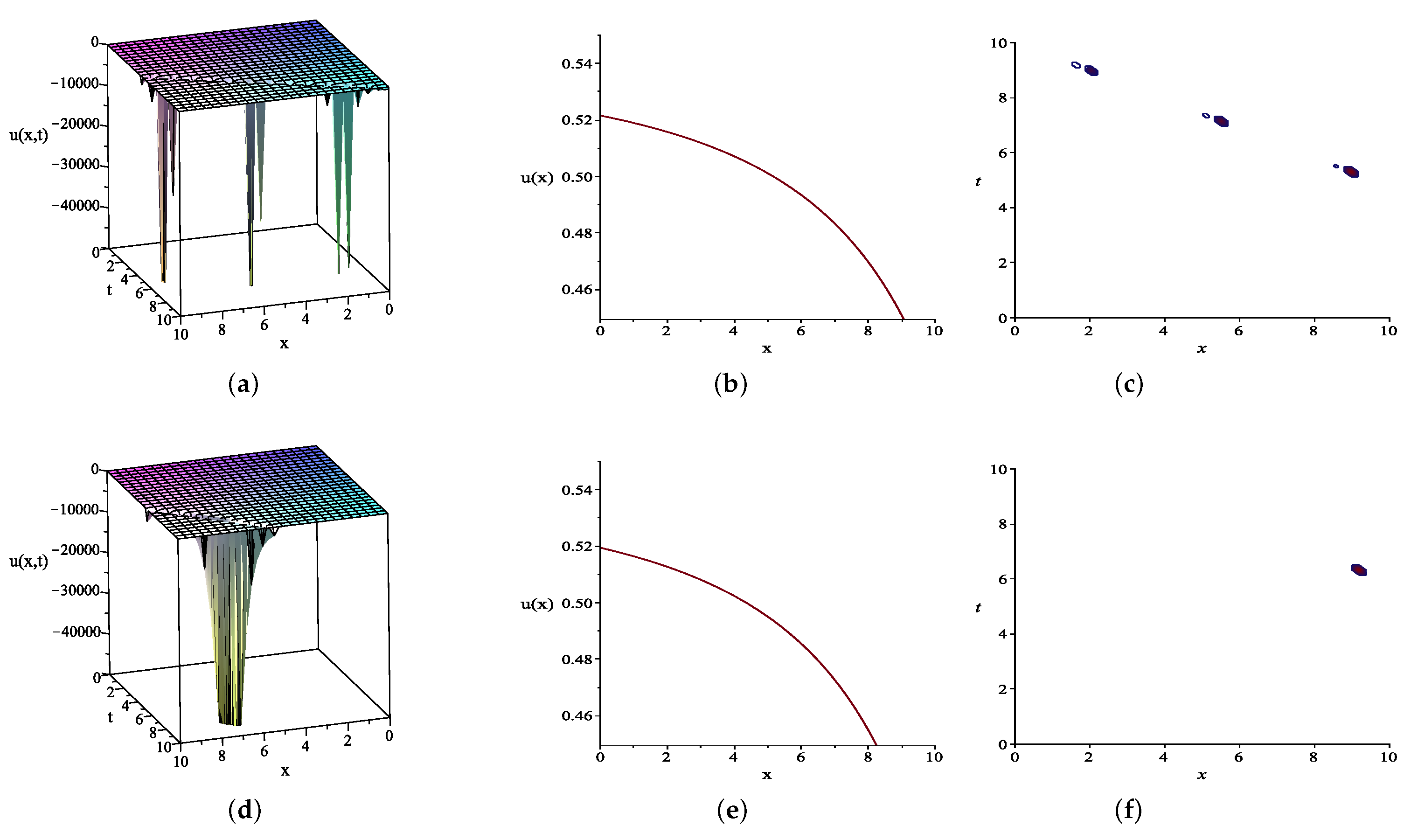
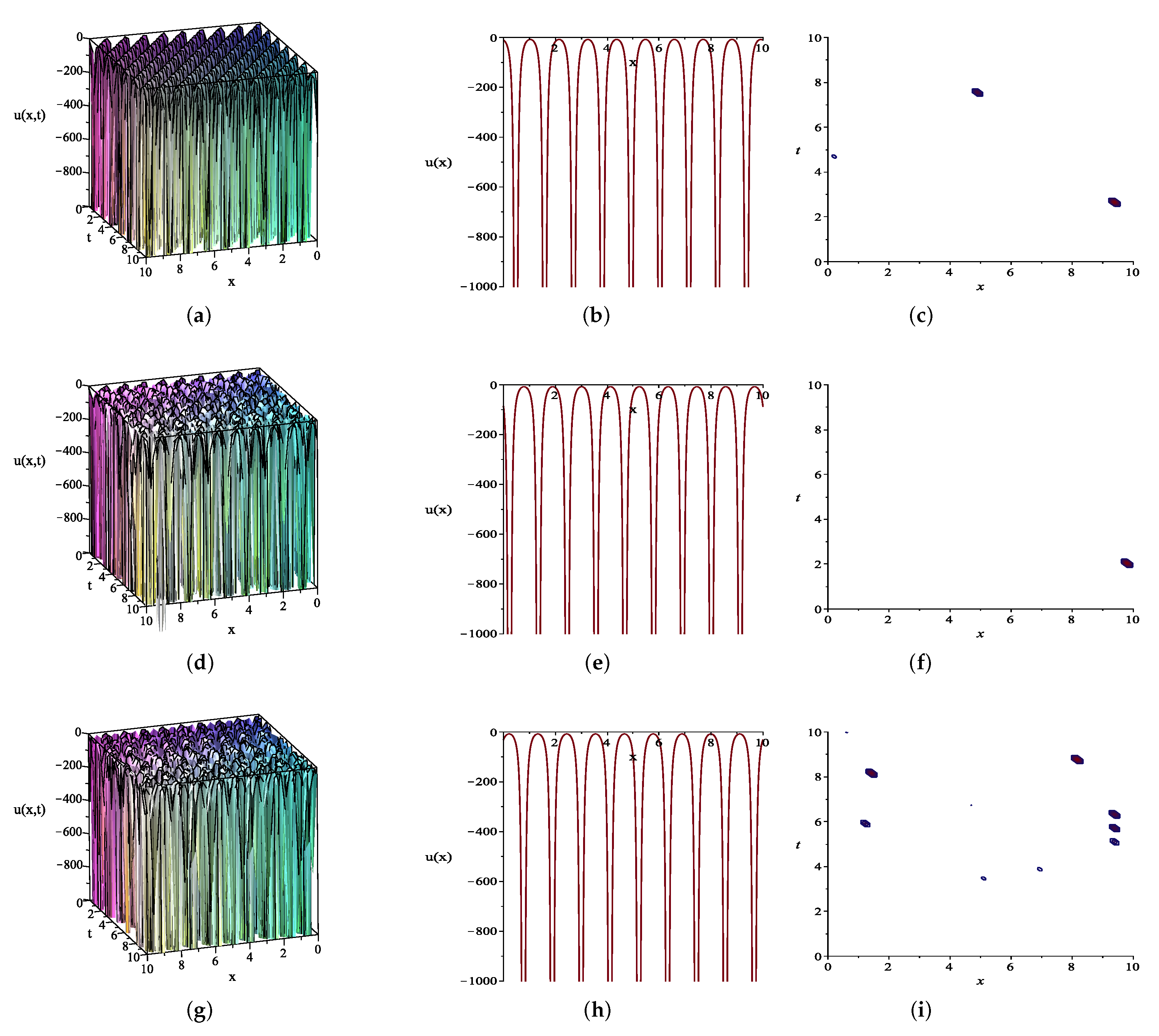
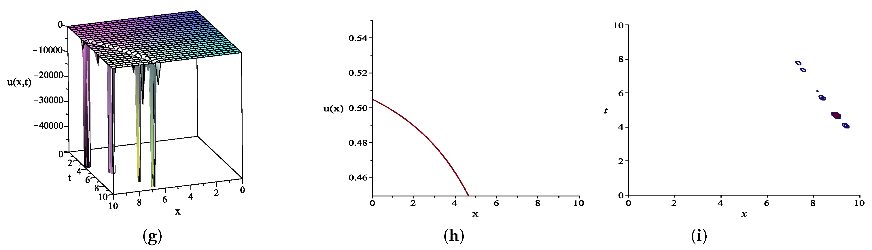
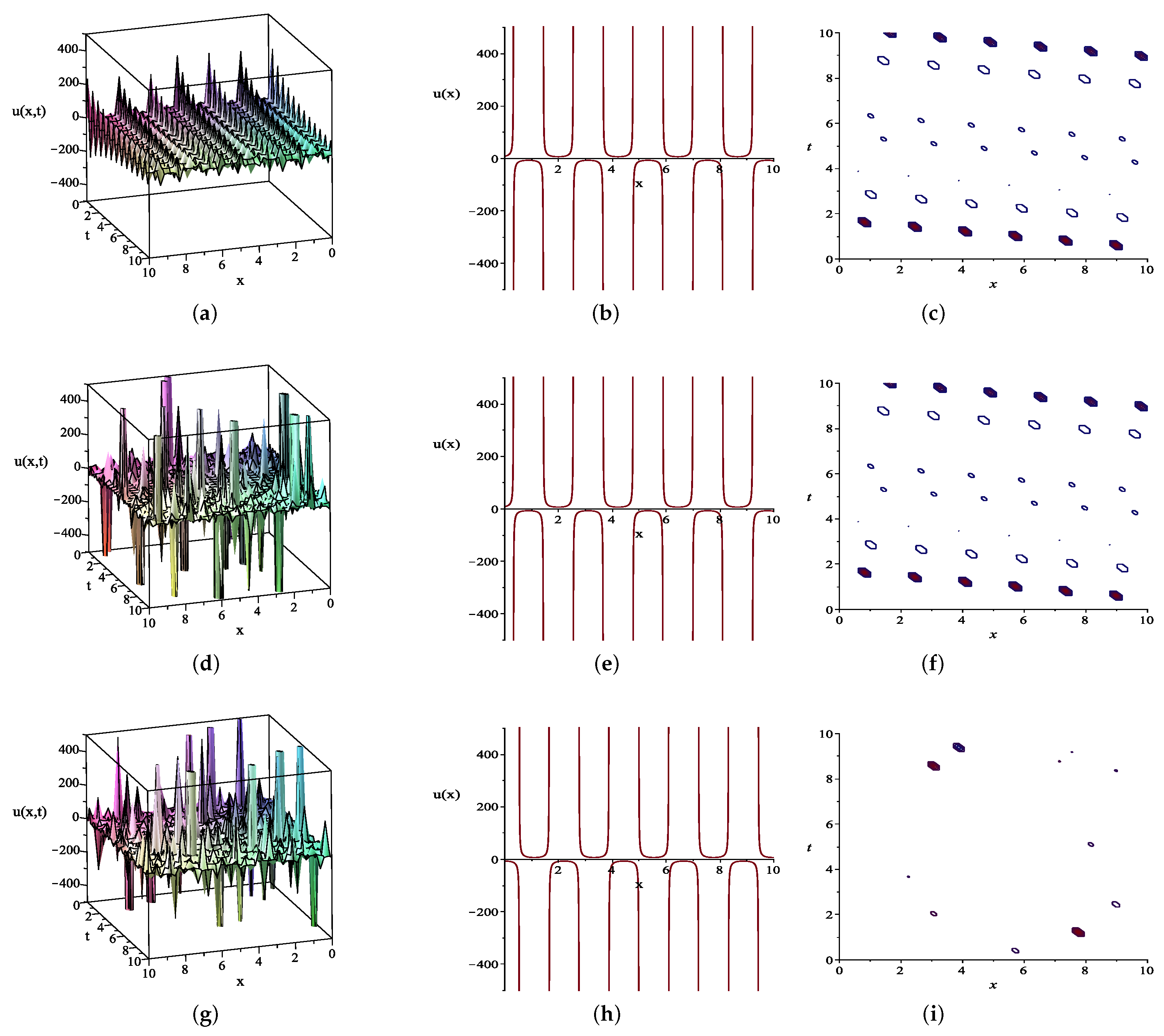
5. Graphical Representations of the Selected Solutions

In this portion, we will manifest interesting graphical representations of the selected exact solutions of the ( 2 + 1 ) -dimensional conformable time integro-differential Sawada–Kotera Equation (1) and of the (3 + 1)-dimensional conformable time modified KdV–Zakharov–Kuznetsov (mKdV–ZK) Equation (2) obtained using the algorithm of the ( G / G 2 ) -expansion method. The time-fractional order α for the equations is changed in order to study graphical behaviors of the exact solutions chosen from the previous section. Particularly, the values of the time-fractional order used for the following simulations are α = 1 , 0.7 and 0.3 . Solutions (41) and (46) of Equation (1) and solution (65) of Equation (2) are selected to present in terms of 3D, 2D, and contour plots according to the values of α . All of the 3D solution graphs of (1) and (2) are portrayed on the domain { ( x , y , t ) : 0 x , t 10 , y = 1 } and { ( x , y , z , t ) : 0 x , t 10 , y = z = 1 } , respectively. The 2D solution graphs, demonstrating a relation between u ( x ) and x, of (1) and (2) are depicted on { ( x , y , t ) : 0 x 10 , y = t = 1 } and { ( x , y , z , t ) : 0 x 10 , y = z = t = 1 } , respectively. Moreover, the contour plots, showing a 3D surface by plotting constant u slices on a 2D plane, are drawn to connect the ( x , t ) coordinates when the values of u are given and y = 1 for (1) but y = z = 1 for (2). In addition, physical descriptions of the displayed graphs will be mentioned in this section.
Figure 1 and Figure 2 show the solution graphs of the exact solutions u 3 2 ( x , y , t ) in (41) and u 1 3 ( x , y , t ) in (46) for problem (1), respectively. They are unfolded in different aspects, i.e., the 3D, 2D, and contour plots. Varying the values of α = 1 , 0.7 , 0.3 , the solutions (41) and (46) are evaluated using the parameter sets { c = 2 , μ = 0 , λ = 1 , C = 0.5 , D = 10 } and { c = 1300 , μ = 2 , λ = 1 , C = 1 , D = 1 } , respectively, to plot their graphs on the domains. Particularly, Figure 1a–c shows the 3D, 2D, and contour plots for solution (41), respectively, when α = 1 . Figure 1d–f and Figure 1g–i are plotted in the same manner as before except using α = 0.7 and α = 0.3 , respectively. By classifying the shapes of the 3D and 2D graphs in Figure 1, it can be identified that solution (41) is a singular single-soliton solution that is a solitary wave with discontinuous derivatives occurring at some domain regions, as observed in the contour plots of Figure 1. In addition, Figure 2a–c shows the 3D, 2D, and contour plots for solution (46), respectively, when α = 1 . Figure 2d–f and Figure 2g–i are drawn in a similar manner to the above plots except using α = 0.7 and α = 0.3 , respectively. As noticed in the 3D and 2D graph structures in Figure 2, their physical behavior is considered as a singular periodic wave solution (or, a singular wavetrain), which is spatiotemporal oscillations with discontinuous derivatives. It can be roughly observed from the 3D graphs that the number of oscillations of the singular periodic wave solutions gradually increases as the fractionality α ( 0 , 1 ) decreases.
The solution graphs of the exact solution u 1 3 , 1 ( x , y , z , t ) in (65) for problem (2) are presented in Figure 3. To be clear, exact solution (65), in which the top sign of ∓ is chosen, is computed utilizing the parameter set { δ 1 = δ 2 = 1 , δ 3 = 1 , ε = β = σ = 1 , μ = 2 , λ = 1 , C = 0.5 , D = 1 } to plot its 3D, 2D, and contour graphs on the domains according to the used values of α . Specifically, Figure 3a–c shows the 3D, 2D, and contour graphs of the solution (65) when α = 1 is used. However, the 3D, 2D, and contour plots of the solution (65) when α = 0.7 and α = 0.3 are exhibited in Figure 3d–f and Figure 3g–i, respectively. The physical behavior of these graphs is characterized as a singularly double periodic wave solution. The significant part of the doubly periodic wave solution represents a traveling wave whose envelope of emerging oscillations is bounded by a pattern periodic in both time and space. In addition, the number of oscillations of this solution type is inversely proportional to the value of α .

6. Conclusions and Future Work

In our study, we have determined closed-form traveling wave solutions for the two nonlinear conformable evolution equations, which are the ( 2 + 1 ) -dimensional conformable time integro-differential SK Equation (1) and the (3 + 1)-dimensional conformable time mKdV–ZK Equation (2) by means of the ( G / G 2 ) -expansion method. After eliminating the trivial and disqualified solutions, Equations (1) and (2) have three main results; each result provides the following three types of solutions: trigonometric, exponential (or, equivalently, hyperbolic), and rational function solutions. All of the exact solutions obtained in this paper were substituted back into their corresponding equations with the help of the Maple package program and their satisfactions confirm the validity of the solutions expressed in the current article. After visualizing the graphs of some solutions, they present some physical behaviors such as the singular single-soliton solution, the singular periodic wave solution and the singularly double periodic wave solution. These characteristics of the solutions are favorable for investigating certain nonlinear phenomena arising in physics, applied mathematics, and engineering. In particular, the soliton is a self-reinforcing wave packet maintaining its shape while propagating at a constant velocity. In other words, solitons are unscathed in shape and speed by a collision with other solitons and are often studied in quantum mechanics, nuclear physics, and waves along a weakly anharmonic mass-spring chain. Moreover, periodic traveling waves play a fundamental role in several mathematical physics including self-oscillatory systems, reaction–diffusion–advection systems, and excitable chemical reactions. Specifically, the family of doubly periodic wave solutions is of great importance in several physical phenomena such as modulation instability applied to the classical nonlinear Schrödinger equation (NLSE) and applications both in optics and deep water waves [64]. Since Equation (1), involving the time conformable partial derivative, is first proposed, then its obtained solutions are new and informed here for the first time. Equation (2) is an extension of the ( 3 + 1 ) -dimensional conformable time mKdV–ZK equation in Equation (48) of [65] for which the coefficients δ 2 and δ 3 are added. It is worth comparing our outcomes for (2) and the exact solutions of Equation (48) of [65] as follows: In [65], the first integral method and the functional variable method were used to solve the equation for which the trigonometric and hyperbolic function solutions were established. The mathematical structures of their results agree with those of our solutions for (2) except the ( G / G 2 ) -expansion method additionally provides the rational function solutions for the equation. In conclusion, the performance of the method is direct, concise, reliable, and effective, and the method gives some interestingly particular types of solutions. Therefore, we deduce that the proposed methods can be extensively employed to solve many conformable NPDEs arising in the theory of solitons or other physics and engineering fields. Lastly, future studies could fruitfully explore the use of the ( G / G 2 ) -expansion method further by applying it to the proposed problems with an extension of the spatiotemporal conformable partial derivatives or to NLEEs involving with sequential conformable partial derivatives.

Author Contributions

Conceptualization, S.S. (Sekson Sirisubtawee), S.K. (Sanoe Koonprasert), and S.S. (Surattana Sungnul); methodology, S.K. (Supaporn Kaewta) and S.S. (Sekson Sirisubtawee); software, S.K. (Supaporn Kaewta) and S.S. (Sekson Sirisubtawee); validation, S.K. (Supaporn Kaewta), S.S. (Sekson Sirisubtawee), S.K. (Sanoe Koonprasert), and S.S. (Surattana Sungnul); formal analysis, S.K. (Supaporn Kaewta) and S.S. (Sekson Sirisubtawee); investigation, S.K. (Supaporn Kaewta), S.S. (Sekson Sirisubtawee), S.K. (Sanoe Koonprasert), and S.S. (Surattana Sungnul); resources, S.S. (Sekson Sirisubtawee) and S.S. (Surattana Sungnul); data curation, S.K. (Supaporn Kaewta); writing—original draft preparation, S.K. (Supaporn Kaewta) and S.S. (Sekson Sirisubtawee); writing—review and editing, S.K. (Supaporn Kaewta), S.S. (Sekson Sirisubtawee), S.K. (Sanoe Koonprasert), and S.S. (Surattana Sungnul); visualization, S.K. (Supaporn Kaewta), S.S. (Sekson Sirisubtawee), and S.S. (Surattana Sungnul); supervision, S.S. (Sekson Sirisubtawee), S.K. (Sanoe Koonprasert), and S.S. (Surattana Sungnul); project administration, S.S. (Sekson Sirisubtawee) and S.S. (Surattana Sungnul); funding acquisition, S.K. (Supaporn Kaewta) and S.S. (Sekson Sirisubtawee). All authors have read and agreed to the published version of the manuscript.

Funding

The first author was funded by King Mongkut’s University of Technology North Bangkok under Contract No. KMUTNB-61-PHD-014. The second author was financially supported by King Mongkut’s University of Technology North Bangkok under Contract No. KMUTNB-62-KNOW-31.

Institutional Review Board Statement

Not applicable.

Informed Consent Statement

Not applicable.

Data Availability Statement

Not applicable.

Acknowledgments

The authors are grateful to anonymous referees for the valuable comments, which have significantly improved this article. In addition, the first author would like to acknowledge the partial support from the Graduate College, King Mongkut’s University of Technology North Bangkok.

Conflicts of Interest

The authors declare no conflict of interest.

References

  1. Lü, X. Madelung fluid description on a generalized mixed nonlinear Schrödinger equation. Nonlinear Dyn. 2015, 81, 239–247. [Google Scholar] [CrossRef]
  2. Lü, X.; Ma, W.X.; Yu, J.; Lin, F.; Khalique, C.M. Envelope bright-and dark-soliton solutions for the Gerdjikov–Ivanov model. Nonlinear Dyn. 2015, 82, 1211–1220. [Google Scholar] [CrossRef]
  3. Seadawy, A.R. Stability analysis solutions for nonlinear three-dimensional modified Korteweg–de Vries–Zakharov–Kuznetsov equation in a magnetized electron–positron plasma. Phys. A Stat. Mech. Appl. 2016, 455, 44–51. [Google Scholar] [CrossRef]
  4. Hayward, R.; Biancalana, F. Constructing new nonlinear evolution equations with supersymmetry. J. Phys. A Math. Theor. 2018, 51, 275202. [Google Scholar] [CrossRef] [Green Version]
  5. Ahmad, I.; Siraj-ul-Islam. Local meshless method for PDEs arising from models of wound healing. Appl. Math. Model. 2017, 48, 688–710. [Google Scholar]
  6. Vakhnenko, V.; Parkes, E. Approach in theory of nonlinear evolution equations: The Vakhnenko-Parkes equation. Adv. Math. Phys. 2016, 2016, 2916582. [Google Scholar] [CrossRef] [Green Version]
  7. Manafian, J. Optical soliton solutions for Schrödinger type nonlinear evolution equations by the tan (Φ (ξ)/2)-expansion method. Optik 2016, 127, 4222–4245. [Google Scholar] [CrossRef]
  8. Bhrawy, A.; Alhuthali, M.S.; Abdelkawy, M. New solutions for (1 + 1)-dimensional and (2 + 1)-dimensional Ito equations. Math. Probl. Eng. 2012, 2012, 537930. [Google Scholar] [CrossRef] [Green Version]
  9. Roshid, M.M.; Roshid, H.O. Exact and explicit traveling wave solutions to two nonlinear evolution equations which describe incompressible viscoelastic Kelvin-Voigt fluid. Heliyon 2018, 4, e00756. [Google Scholar] [CrossRef] [Green Version]
  10. Bustamante-Castañeda, F.; Caputo, J.G.; Cruz-Pacheco, G.; Knippel, A.; Mouatamide, F. Epidemic model on a network: Analysis and applications to COVID-19. Phys. A Stat. Mech. Appl. 2021, 564, 125520. [Google Scholar] [CrossRef]
  11. Ghafoor, A.; Firdous, S.; Zubair, T.; Iftikhar, A.; Zainab, S.; Mohyud-Din, S.T. (G′/G,1/G)–Expansion method for generalized ZK, Sharma–Tasso–Olver (STO) and modified ZK equations. QSci. Connect 2013, 2013, 24. [Google Scholar] [CrossRef]
  12. Hossain, A.K.S.; Akbar, M.A. Traveling wave solutions of Benny Luke equation via the enhanced (G’/G)-expansion method. Ain Shams Eng. J. 2021. [Google Scholar] [CrossRef]
  13. He, J.H. Exp-function method for fractional differential equations. Int. J. Nonlinear Sci. Numer. Simul. 2013, 14, 363–366. [Google Scholar] [CrossRef]
  14. Zheng, B.; Feng, Q. The Jacobi elliptic equation method for solving fractional partial differential equations. In Abstract and Applied Analysis; Hindawi: London, UK, 2014; Volume 2014. [Google Scholar]
  15. Biswas, A.; Sonmezoglu, A.; Ekici, M.; Mirzazadeh, M.; Zhou, Q.; Moshokoa, S.P.; Belic, M. Optical soliton perturbation with fractional temporal evolution by generalized Kudryashov’s method. Optik 2018, 164, 303–310. [Google Scholar] [CrossRef]
  16. Baskonus, H.M.; Sulaiman, T.A.; Bulut, H. Novel complex and hyperbolic forms to the strain wave equation in microstructured solids. Opt. Quantum Electron. 2018, 50, 14. [Google Scholar] [CrossRef]
  17. Mohyud-Din, S.T.; Nawaz, T.; Azhar, E.; Akbar, M.A. Fractional sub-equation method to space–time fractional Calogero-Degasperis and potential Kadomtsev-Petviashvili equations. J. Taibah Univ. Sci. 2017, 11, 258–263. [Google Scholar] [CrossRef] [Green Version]
  18. Manafian, J.; Foroutan, M. Application of tan(ϕ(ξ)/2)-expansion method for the time-fractional Kuramoto–Sivashinsky equation. Opt. Quantum Electron. 2017, 49, 272. [Google Scholar] [CrossRef]
  19. Seadawy, A.R. Three-dimensional nonlinear modified Zakharov–Kuznetsov equation of ion-acoustic waves in a magnetized plasma. Comput. Math. Appl. 2016, 71, 201–212. [Google Scholar] [CrossRef]
  20. Seadawy, A.R. Solitary wave solutions of two-dimensional nonlinear Kadomtsev–Petviashvili dynamic equation in dust-acoustic plasmas. Pramana 2017, 89, 49. [Google Scholar] [CrossRef]
  21. Zhouzheng, K. G′/G2-expansion Solutions to MBBM and OBBM Equations. J. Part. Differ. Equ. 2015, 28, 158–166. [Google Scholar] [CrossRef]
  22. Mohyud-Din, S.T.; Bibi, S. Exact solutions for nonlinear fractional differential equations using G′/G2-expansion method. Alex. Eng. J. 2018, 57, 1003–1008. [Google Scholar] [CrossRef]
  23. Arshed, S.; Sadia, M. (G′/G2)-Expansion method: New traveling wave solutions for some nonlinear fractional partial differential equations. Opt. Quantum Electron. 2018, 50, 123. [Google Scholar] [CrossRef]
  24. Sirisubtawee, S.; Koonprasert, S. Exact traveling wave solutions of certain nonlinear partial differential equations using the (G′/G2)-expansion method. Adv. Math. Phys. 2018, 2018, 7628651. [Google Scholar] [CrossRef] [Green Version]
  25. Meng, Y. Expanded G′/G2-expansion method to solve separated variables for the (2 + 1)-dimensional NNV equation. Adv. Math. Phys. 2018, 2018, 9248174. [Google Scholar] [CrossRef]
  26. Ali, M.N.; Osman, M.; Husnine, S.M. On the analytical solutions of conformable time-fractional extended Zakharov–Kuznetsov equation through G′/G2-expansion method and the modified Kudryashov method. SeMA J. 2019, 76, 15–25. [Google Scholar] [CrossRef]
  27. Kaewta, S.; Sirisubtawee, S.; Khansai, N. Explicit exact solutions of the (2 + 1)-dimensional integro-differential Jaulent–Miodek evolution equation using the reliable methods. Int. J. Math. Math. Sci. 2020, 2020. [Google Scholar] [CrossRef]
  28. Devi, P.; Singh, K. Exact traveling wave solutions of the (2 + 1)-dimensional Boiti-Leon-Pempinelli system using G′/G2-expansion method. In AIP Conference Proceedings; AIP Publishing LLC: Melville, NY, USA, 2020; Volume 2214, p. 020030. [Google Scholar]
  29. Bilal, M.; Seadawy, A.R.; Younis, M.; Rizvi, S.; Zahed, H. Dispersive of propagation wave solutions to unidirectional shallow water wave Dullin–Gottwald–Holm system and modulation instability analysis. Math. Methods Appl. Sci. 2021, 44, 4094–4104. [Google Scholar] [CrossRef]
  30. Shi, Y.; Li, D. New exact solutions for the (2 + 1)-dimensional Sawada–Kotera equation. Comput. Fluids 2012, 68, 88–93. [Google Scholar] [CrossRef]
  31. Zhao, Z.; Zhang, Y.; Xia, T. Double periodic wave solutions of the (2 + 1)-dimensional Sawada-Kotera equation. Abstr. Appl. Anal. 2014, 2014, 534017. [Google Scholar] [CrossRef]
  32. Li, X.; Wang, Y.; Chen, M.; Li, B. Lump solutions and resonance stripe solitons to the (2 + 1)-dimensional Sawada-Kotera equation. Adv. Math. Phys. 2017, 2017, 1743789. [Google Scholar] [CrossRef] [Green Version]
  33. Zhang, H.Q.; Ma, W.X. Lump solutions to the (2 + 1)-dimensional Sawada–Kotera equation. Nonlinear Dyn. 2017, 87, 2305–2310. [Google Scholar] [CrossRef]
  34. Hu, R. Diversity of interaction solutions to the (2 + 1)-dimensional Sawada-Kotera equation. J. Appl. Math. Phys. 2018, 6, 1692. [Google Scholar] [CrossRef] [Green Version]
  35. An, H.; Feng, D.; Zhu, H. General M-lump, high-order breather and localized interaction solutions to the (2 + 1)-dimensional Sawada–Kotera equation. Nonlinear Dyn. 2019, 98, 1275–1286. [Google Scholar] [CrossRef]
  36. Ghanbari, B.; Kuo, C.K. A variety of solitary wave solutions to the (2 + 1)-dimensional bidirectional SK and variable-coefficient SK equations. Results Phys. 2020, 18, 103266. [Google Scholar] [CrossRef]
  37. Konopelchenko, B.; Dubrovsky, V. Some new integrable nonlinear evolution equations in (2 + 1)-dimensions. Phys. Lett. A 1984, 102, 15–17. [Google Scholar] [CrossRef]
  38. Sawada, K.; Kotera, T. A method for finding N-soliton solutions of the KdV equation and KdV-like equation. Prog. Theor. Phys. 1974, 51, 1355–1367. [Google Scholar] [CrossRef] [Green Version]
  39. Lou, S.Y. Symmetries of the KdV equation and four hierarchies of the integrodifferential KdV equations. J. Math. Phys. 1994, 35, 2390–2396. [Google Scholar] [CrossRef]
  40. Xu, Z.; Chen, H.; Chen, W. The multisoliton solutions for the (2 + 1)-dimensional Sawada-Kotera equation. Abstr. Appl. Anal. 2013, 2013, 767254. [Google Scholar] [CrossRef] [Green Version]
  41. Lu, D.; Seadawy, A.; Arshad, M.; Wang, J. New solitary wave solutions of (3 + 1)-dimensional nonlinear extended Zakharov-Kuznetsov and modified KdV-Zakharov-Kuznetsov equations and their applications. Results Phys. 2017, 7, 899–909. [Google Scholar] [CrossRef]
  42. Lu, D.; Seadawy, A.; Yaro, D. Analytical wave solutions for the nonlinear three-dimensional modified Korteweg-de Vries-Zakharov-Kuznetsov and two-dimensional Kadomtsev-Petviashvili-Burgers equations. Results Phys. 2019, 12, 2164–2168. [Google Scholar] [CrossRef]
  43. Tariq, K.U.H.; Seadawy, A. Soliton solutions of (3 + 1)–dimensional Korteweg-de Vries Benjamin–Bona–Mahony, Kadomtsev–Petviashvili Benjamin–Bona–Mahony and modified Korteweg de Vries–Zakharov–Kuznetsov equations and their applications in water waves. J. King Saud Univ.-Sci. 2019, 31, 8–13. [Google Scholar] [CrossRef]
  44. Naher, H.; Abdullah, F.A.; Akbar, M.A. Generalized and improved G′/G-expansion method for (3 + 1)-dimensional modified KdV-Zakharov-Kuznetsev equation. PLoS ONE 2013, 8, e64618. [Google Scholar] [CrossRef] [PubMed]
  45. Islam, M.H.; Khan, K.; Akbar, M.A.; Salam, M.A. Exact traveling wave solutions of modified KdV–Zakharov–Kuznetsov equation and viscous Burgers equation. SpringerPlus 2014, 3, 105. [Google Scholar] [CrossRef] [Green Version]
  46. Miah, M.M.; Ali, H.S.; Akbar, M.A.; Seadawy, A.R. New applications of the two variable (G’/G, 1/G)-expansion method for closed form traveling wave solutions of integro-differential equations. J. Ocean Eng. Sci. 2019, 4, 132–143. [Google Scholar] [CrossRef]
  47. Gepreel, K.A.; Nofal, T.A.; Alasmari, A.A. Exact solutions for nonlinear integro-partial differential equations using the generalized Kudryashov method. J. Egypt. Math. Soc. 2017, 25, 438–444. [Google Scholar] [CrossRef]
  48. Guner, O.; Aksoy, E.; Bekir, A.; Cevikel, A.C. Different methods for (3 + 1)-dimensional space–time fractional modified KdV–Zakharov–Kuznetsov equation. Comput. Math. Appl. 2016, 71, 1259–1269. [Google Scholar] [CrossRef]
  49. Islam, M.T.; Akbar, M.A.; Azad, M.A.K. Traveling wave solutions in closed form for some nonlinear fractional evolution equations related to conformable fractional derivative. AIMS Math. 2018, 3, 625–646. [Google Scholar] [CrossRef]
  50. Guner, O. New exact solutions to the space–time fractional nonlinear wave equation obtained by the ansatz and functional variable methods. Opt. Quantum Electron. 2018, 50, 38. [Google Scholar] [CrossRef]
  51. Al-Ghafri, K.; Rezazadeh, H. Solitons and other solutions of (3 + 1)-dimensional space–time fractional modified KdV–Zakharov–Kuznetsov equation. Appl. Math. Nonlinear Sci. 2019, 4, 289–304. [Google Scholar] [CrossRef] [Green Version]
  52. Khalil, R.; Al Horani, M.; Yousef, A.; Sababheh, M. A new definition of fractional derivative. J. Comput. Appl. Math. 2014, 264, 65–70. [Google Scholar] [CrossRef]
  53. Chung, W.S. Fractional Newton mechanics with conformable fractional derivative. J. Comput. Appl. Math. 2015, 290, 150–158. [Google Scholar] [CrossRef]
  54. Çenesiz, Y.; Baleanu, D.; Kurt, A.; Tasbozan, O. New exact solutions of Burgers’ type equations with conformable derivative. Waves Random Complex Media 2017, 27, 103–116. [Google Scholar] [CrossRef]
  55. Sirisubtawee, S.; Koonprasert, S.; Sungnul, S. Some applications of the (G′/G,1/G)-expansion method for finding exact traveling wave solutions of nonlinear fractional evolution equations. Symmetry 2019, 11, 952. [Google Scholar] [CrossRef] [Green Version]
  56. Sirisubtawee, S.; Koonprasert, S.; Sungnul, S.; Leekparn, T. Exact traveling wave solutions of the space–time fractional complex Ginzburg–Landau equation and the space-time fractional Phi-4 equation using reliable methods. Adv. Differ. Equ. 2019, 2019, 219. [Google Scholar] [CrossRef]
  57. Sirisubtawee, S.; Koonprasert, S.; Sungnul, S. New exact solutions of the conformable space-time Sharma–Tasso–Olver equation using two reliable methods. Symmetry 2020, 12, 644. [Google Scholar] [CrossRef] [Green Version]
  58. Al-Ghafri, K.S. Soliton behaviours for the conformable space–time fractional complex Ginzburg–Landau equation in optical fibers. Symmetry 2020, 12, 219. [Google Scholar] [CrossRef] [Green Version]
  59. Hosseini, K.; Manafian, J.; Samadani, F.; Foroutan, M.; Mirzazadeh, M.; Zhou, Q. Resonant optical solitons with perturbation terms and fractional temporal evolution using improved tan (ϕ (η)/2)-expansion method and exp function approach. Optik 2018, 158, 933–939. [Google Scholar] [CrossRef]
  60. Abdeljawad, T. On conformable fractional calculus. J. Comput. Appl. Math. 2015, 279, 57–66. [Google Scholar] [CrossRef]
  61. Kumar, D.; Darvishi, M.; Joardar, A. Modified Kudryashov method and its application to the fractional version of the variety of Boussinesq-like equations in shallow water. Opt. Quantum Electron. 2018, 50, 128. [Google Scholar] [CrossRef]
  62. El-Ajou, A.; Al-Zhour, Z.; Oqielat, M.; Momani, S.; Hayat, T. Series solutions of nonlinear conformable fractional KdV-Burgers equation with some applications. Eur. Phys. J. Plus 2019, 134, 402. [Google Scholar] [CrossRef]
  63. Chen, J.; Chen, H. The G′/G2-expansion method and its application to coupled nonlinear Klein-Gordon equation. J. South China Norm. Univ. (Nat. Sci. Ed.) 2012, 44, 13. [Google Scholar]
  64. Conforti, M.; Mussot, A.; Kudlinski, A.; Trillo, S.; Akhmediev, N. Doubly periodic solutions of the focusing nonlinear Schrödinger equation: Recurrence, period doubling, and amplification outside the conventional modulation-instability band. Phys. Rev. A 2020, 101, 023843. [Google Scholar] [CrossRef] [Green Version]
  65. Eslami, M.; Rezazadeh, H.; Rezazadeh, M.; Mosavi, S.S. Exact solutions to the space–time fractional Schrödinger–Hirota equation and the space–time modified KDV–Zakharov–Kuznetsov equation. Opt. Quantum Electron. 2017, 49, 279. [Google Scholar] [CrossRef]
Figure 1. Associated plots of the solution u 3 2 ( x , y , t ) in Equation (41) obtained using the ( G / G 2 ) -expansion method: (ac) 3D plot, 2D plot, and contour plot when α = 1 ; (df) 3D plot, 2D plot, and contour plot when α = 0.7 ; (gi) 3D plot, 2D plot, and contour plot when α = 0.3 .
Fractalfract 05 00088 g001aFractalfract 05 00088 g001b
Figure 2. Associated plots of the solution u 1 3 ( x , y , t ) in Equation (46) obtained using the ( G / G 2 ) -expansion method: (ac) 3D plot, 2D plot, and contour plot when α = 1 ; (df) 3D plot, 2D plot, and contour plot when α = 0.7 ; (gi) 3D plot, 2D plot, and contour plot when α = 0.3 .
Fractalfract 05 00088 g002
Figure 3. Associated plots of the solution u 1 3 , 1 ( x , y , z , t ) in Equation (65) obtained using the ( G / G 2 ) -expansion method: (ac) 3D plot, 2D plot, and contour plot when α = 1 ; (df) 3D plot, 2D plot, and contour plot when α = 0.7 ; (gi) 3D plot, 2D plot, and contour plot when α = 0.3 .
Fractalfract 05 00088 g003
Table 1. Sign of u ( x , y , z , t ) selected from ± or ∓ in front of u ( x , y , z , t ) .
ResultSign of a 1 Sign of b 1 Sign Selected from ± or ∓ in Front of u ( x , y , z , t )
μ λ > 0 μ λ < 0 μ = 0 , λ 0
3.1++
+++
3.2+++
++
Publisher’s Note: MDPI stays neutral with regard to jurisdictional claims in published maps and institutional affiliations.

