Pseudo-Likelihood Estimation for Parameters of Stochastic Time-Fractional Diffusion Equations

Abstract

Although stochastic fractional partial differential equations have received increasing attention in the last decade, the parameter estimation of these equations has been seldom reported in literature. In this paper, we propose a pseudo-likelihood approach to estimating the parameters of stochastic time-fractional diffusion equations, whose forward solver has been investigated very recently by Gunzburger, Li, and Wang (2019). Our approach can accurately recover the fractional order, diffusion coefficient, as well as noise magnitude given the discrete observation data corresponding to only one realization of driving noise. When only partial data is available, our approach can also attain acceptable results for intermediate sparsity of observation.

1. Introduction

Stochastic fractional partial differential equations (SFPDEs) have received a fair amount of attention in the last decade. Research in that direction involves constructing new SFPDE models, proving well-posedness of model solution, and developing new numerical solution methods. Some of the SFPDEs can be written in the following general form:

$${\partial }_t^{\beta }u(x,t)=-c{(-\Delta )}^{\tilde{\alpha }\left(x\right)/2}u(x,t)+f(x,t)+ϵI_t^{1-\beta }\left(\sigma \left(u\right)\dot{W}(x,t)\right),$$

(1)

where $\beta$ is the order of Caputo fractional time derivative, c is diffusion coefficient, $\tilde{\alpha }\left(x\right)$ is the spatially variable order of fractional Laplacian, $f(x,t)$ is a prescribed source term and $I_t^{1-\beta }$ is fractional time integration operator, $\dot{W}(x,t)$ is a space-time white noise, and $ϵ$ is the magnitude of the noise. Mijena and Nane [1] proved the existence and uniqueness of mild solutions to the space-time fractional nonlinear PDE (1) with $\beta \in (0,1)$, $\tilde{\alpha }\left(x\right)\equiv \alpha$, and a Lipschitz continuous $\sigma (·)$. Anh, Leonenko, and Ruiz-Medina [2] derived the weak-sense Gaussian solution to the SFPDE (1) with $\beta \in (0,1)$, $\sigma (·)\equiv 1$, and pseudo-differential operator ${(-\Delta )}^{\tilde{\alpha }\left(x\right)/2}$. Gunzburger, Li, and Wang [3] proposed a time discretization scheme for stochastic time-fractional PDE (1) with $\beta \in (0,1),\tilde{\alpha }\left(x\right)\equiv 2$, and $\sigma (·)\equiv 1$. Some other authors considered SFPDEs that differ from the general form (1). Bolin, Kirchner, and Kovács [4] presented a numerical solution method for an elliptic SFPDE ${(\kappa -\Delta )}^{\beta }u\left(x\right)=W\left(x\right)$, where $W\left(x\right)$ is a Gaussian white noise. Anh, Olenko, and Wang [5] constructed a SFPDE to model the evolution of a random tangent vector field on the unit sphere. Mohammed [6] and Xia and Yan [7] considered FPDEs driven by multiplicative Brownian motion and fractional Brownian motion, respectively.

In contrast to the rapid development of numerical solution to forward problems, parameter estimation for SFPDEs has not yet been fully investigated, although there have been many works on parameter estimation for SPDEs [8,9,10,11]. Cialenco, Lototsk, and Pospisil [12] and Cialenco [13] studied the parameter estimation of diffusion coefficient and Hurst index for standard (integer-order) diffusion driven by additive and multiplicative fractional noises. When the fractional ingredient in the driving noise is excluded, the equations they considered are more like stochastic integer-order PDEs, which are not of the concern of current study. Geldhauser and Valdinociun [14] did consider a SFPDE, and they estimated the order of fractional Laplacian in the context of optimal control.

Parameter estimation for deterministic and stochastic FPDEs are different. Inversion for deterministic FPDEs often involves solving forward problems, while inversion for stochastic FPDE does not. Specifically, for deterministic FPDEs, once the source term $f(x,t)$ and initial/boundary conditions are known, one can solve forward problems under different equation parameters, and after utilizing certain inversion techniques such as regularizing nonlinear least squares [15], surrogate models [16,17,18] and physics-informed deep learning [19], one can select the parameters that reconstruct the observation of u as the estimated parameters. For stochastic FPDEs, however, one does not know the specific realization of noise that corresponds to the observation, and thus cannot solve the forward problems even though other conditions are prescribed. Maximum likelihood estimation (MLE) is a powerful means to handle the parameter estimation problems for SPDEs, which can bypass solving forward problems. To the best of our knowledge, there are very few reports on MLE and its variants for parameter estimation of SFPDEs. On the other hand, there have been some efforts on theoretical analyses, such as consistency and asymptotic efficiency, for maximum likelihood estimators for parameters in SPDEs, for example, in [8,11], but the corresponding numerical studies are fewer than the theoretical studies.

In this paper, we propose a pseudo-likelihood estimation approach for SFPDE (1) with $\beta \in (0,1),\tilde{\alpha }\left(x\right)\equiv 2$, and $\sigma (·)\equiv 1$. We extend the pseudo-likelihood approach for solving stochastic ordinary differential equations (SODEs) to SFPDEs, despite the fact that the extension is not trivial. The paper is organized as follows. Section 2 introduces the SFPDE we consider and defines the parameter estimation problem. Section 3 elaborates on pseudo-likelihood approach for the SFPDE, before which we briefly review the approach for SODEs since it inspires us. Section 4 demonstrates some numerical results for fabricated observation data. The last section gives some remarks on the proposed approach.

2. Parameter Estimation Problem

We consider a one-dimensional stochastic time-fractional diffusion problem [3]

$$\left\{\begin{array}{cc}{\partial }_{t}u(x,t)-c\Delta {\partial }_t^{1-\alpha }u(x,t)=f(x,t)+ϵ{\partial }_{t}W(x,t),\hfill & \hfill (x,t)\in {(0,1)}^2,\\ u(0,t)=u(1,t)=0,\hfill & \hfill t\in (0,1),\\ u(x,0)=\eta \left(x\right),\hfill & \hfill x\in (0,1),\end{array}\right.$$

(2)

where $u(x,t)$ is a space-time distribution of concentration of certain particles, the diffusion coefficient $c>0$, the fractional order $\alpha \in (0,1)$, and the initial condition $\eta \left(x\right)$ and the source term $f(x,t)$ are prescribed. The stochastic fractional PDE is driven by a space-time white noise ${\partial }_{t}W(x,t):=\dot{W}(x,t)$, which is the time derivative of a cylindrical Wiener process $W(x,t)$ in $L^2\left((0,1)\right)$ defined by [20]

$$W(x,t)=\sum _{j=1}^{+\infty }{\varphi }_j\left(x\right)W_j\left(t\right),$$

(3)

with ${\varphi }_j\left(x\right)$ being the normalized eigenfunction of negative Laplacian $-\Delta$, i.e., ${\varphi }_j\left(x\right)=\sqrt{2}sin\left(j\pi x\right)$ for $x\in (0,1)$ and ${\left\{W_j\left(t\right)\right\}}_{j=1}^{+\infty }$ being independent one-dimensional Wiener processes. The positive constant $ϵ$ before the white noise determines the noise magnitude. The domain of Laplacian $\Delta$ is $\{\psi \in H_0^1\left((0,1)\right):\Delta \psi \in L^2\left((0,1)\right)$. The left-sided Caputo fractional time derivative is considered:

$${\partial }_t^{1-\alpha }\psi (x,t)=\frac{1}{\Gamma \left(\alpha \right)}{\int }_0^t{(t-s)}^{\alpha -1}{\partial }_s\psi (x,s)\mathrm{d}s,\alpha \in (0,1),$$

(4)

where $\Gamma \left(\alpha \right)$ is the Gamma function. Note that for $\psi (x,0)=0$ the left-sided Caputo fractional time derivative is equivalent to left-sided Riemann–Liouville fractional time derivative. Moreover, applying fractional integration operator ${\partial }_t^{\alpha -1}$ to both hand sides of Equation (2) yields an equivalent equation

$${\partial }_t^{\alpha }u(x,t)-c\Delta (u(x,t)-\eta \left(x\right))={\partial }_t^{\alpha -1}(f(x,t)+ϵ\dot{W}(x,t)),$$

(5)

in which we have used the identity (cf. Lemma 2.22 in [21]) ${\partial }_t^{\alpha -1}{\partial }_t^{1-\alpha }\psi (x,t)=\psi (x,t)-\psi (x,0)$.

The parameter estimation problem can be defined as follows. Given the concentration data $\overline{u}(x_i,t_n)$ observed at space-time grid points $(x_i,t_n)$, we will find the parameters $(c,\alpha ,ϵ)$ that maximize the probability that such concentration data are observed. Notice that we do not know what specific sample (or realization) of the white noise $\dot{W}(x,t)$ corresponds to the current observation, but we only know the observation. We will estimate the magnitude $ϵ$ of the noise only utilizing the observation.

3. Pseudo-Likelihood Approach

In this section, we first review the pseudo-likelihood approach for parameter estimation of stochastic ODEs discussed in Section 3.2 of [22] and then embark on the extension of the approach to stochastic PDEs.

3.1. Pseudo-Likelihood Estimation for Stochastic ODEs

We take the parameter estimation of the following Black-Scholes equation as an example:

$${\partial }_{t}X\left(t\right)={\theta }_{1}X\left(t\right)+{\theta }_{2}X\left(t\right)\dot{W}\left(t\right),{\theta }_1\in \mathbb{R},{\theta }_2>0,$$

(6)

with deterministic intial value $X\left(t_0\right)=x_0$ and Wiener process $W\left(t\right)$. Given the observation $\overline{X}\left(t_n\right)$ for $n=1,2,\cdots ,N$, we will estimate the parameters $({\theta }_1,{\theta }_2)$.

Denote by $p_{{\theta }_1,{\theta }_2}(x_2,s_2|x_1,s_1)$ ($s_1<s_2$) the conditional density of the random variable $X\left(s_2\right)$ given $X\left(s_1\right)$, and the likelihood function for the observation $\left\{\overline{X}\left(t_n\right)\right\}$ is

$$L({\theta }_1,{\theta }_2)=\prod _{n=1}^N{p}_{{\theta }_1,{\theta }_2}(\overline{X}\left(t_n\right),t_n|\overline{X}\left(t_{n-1}\right),t_{n-1}).$$

(7)

The MLE $({\widehat{\theta }}_1,{\widehat{\theta }}_2)$ satisfies

$$({\widehat{\theta }}_1,{\widehat{\theta }}_2)=\underset{{\theta }_1,{\theta }_2}{argmin}\{-logL({\theta }_1,{\theta }_2)\}.$$

(8)

When the explicit form of conditional density is known, the corresponding approach is called exact-likelihood approach. For instance, as the conditional density for Black–Scholes equation is the density of a log-normal random variable [22], we can employ the exact-likelihood approach to infer the parameters. For general diffusion processes, however, the conditional density may not be known explicitly. In this case, we can infer parameters using pseudo-likelihood approach instead.

To make pseudo-likelihood estimation, we need to discretize the SODEs first. We still consider the Black–Scholes equation, and discretize it using the Euler scheme

$$X\left(t_n\right)-X\left(t_{n-1}\right)={\theta }_{1}X\left(t_{n-1}\right)\Delta t+{\theta }_{2}X\left(t_{n-1}\right)(W\left(t_n\right)-W\left(t_{n-1}\right)),$$

(9)

for $n=1,2,\cdots ,N$. As the increment of the Wiener process $W\left(t_n\right)-W\left(t_{n-1}\right)$ is a normal random variable with zero mean and variance $t_n-t_{n-1}$, namely, $W\left(t_n\right)-W\left(t_{n-1}\right)\sim N(0,\Delta t)$, we see that the residual $X\left(t_n\right)-X\left(t_{n-1}\right)-{\theta }_{1}X\left(t_{n-1}\right)\Delta t:=Y_n$ is a normal random variable

$$Y_n\sim N(0,{\theta }_2^2{X}^2\left(t_{n-1}\right)\Delta t).$$

(10)

Thus, the probability we jointly observe ${\overline{Y}}_n=\overline{X}\left(t_n\right)-\overline{X}\left(t_{n-1}\right)-{\theta }_1\overline{X}\left(t_{n-1}\right)\Delta t$ is determined by the density,

$$q_{{\theta }_1,{\theta }_2}(y={\overline{Y}}_n)=\frac{1}{\sqrt{2\pi {\theta }_2^2{\overline{X}}^2\left(t_{n-1}\right)\Delta t}}exp\left\{-\frac{1}{2}\frac{{\overline{Y}}_n^2}{{\theta }_2^2{\overline{X}}^2\left(t_{n-1}\right)\Delta t}\right\}.$$

(11)

Then, the joint probability we observe ${\left\{\overline{X}\left(t_n\right)\right\}}_{n=1}^N$ is

$$\tilde{L}({\theta }_1,{\theta }_2)=\prod _{n=1}^N{q}_{{\theta }_1,{\theta }_2}\left({\overline{Y}}_n\right).$$

(12)

The pseudo-likelihood estimation satisfies

$$({\widehat{\theta }}_1,{\widehat{\theta }}_2)=\underset{{\theta }_1,{\theta }_2}{argmin}\{-log\tilde{L}({\theta }_1,{\theta }_2)\}.$$

(13)

The conditional density $q_{{\theta }_1,{\theta }_2}$ in pseudo-likelihood (12) generally differs from the true conditional density $p_{{\theta }_1,{\theta }_2}$ in (7) as mentioned in preceding paragraphs. The approximation q to p is good when the sampling step $\Delta t$ is very small. For example, for $N{(\Delta t)}^3\to 0$ as $N\to +\infty$ the maximum likelihood estimator built upon pseudo-likelihood is consistent and asymptotically normal [23].

3.2. Pseudo-Likelihood Estimation for Stochastic PDEs

We now consider the parameter estimation of fractional order $\alpha$, diffusion coefficient c, as well as noise magnitude $ϵ$ in problem (2) by leveraging the pseudo-likelihood approach we reviewed in the last subsection. Recalling that the first step we implement the approach is to discretize the Black–Scholes equation using the Euler scheme, we, first of all, need to seek a proper discretization scheme for our stochastic fractional PDE.

3.2.1. Spatio-Temporal Discretization Scheme

We adopt the time discretization scheme proposed in [3] and central difference for temporal and spatial discretizations, respectively. For the computational domain $\{(x,t):(x,t)\in {(0,1)}^2\}$ of problem (2), we denote by $x_i=\frac{i}{N_x},i=0,1,\cdots ,N_x$ the spatial grid and by $t_n=\frac{n}{N_t},n=0,1,\cdots ,N_t$ the temporal grid. The problem (2) can be discretized as

$$\begin{array}{c}\frac{U_i^n-U_i^{n-1}}{\Delta t}-c{(\Delta t)}^{\alpha -1}\sum _{j=0}^n{b}_{n-j,1-\alpha }\frac{U_{i+1}^j-2U_i^j+U_{i-1}^j}{{(\Delta x)}^2}\hfill \\ \hfill \hspace{1em}\hspace{1em}\hspace{1em}\hspace{1em}\hspace{1em}\hspace{1em}\hspace{1em}\hspace{1em}\hspace{1em}\hspace{1em}\hspace{1em}\hspace{1em}\hspace{1em}\hspace{1em}\hspace{1em}\hspace{1em} =F_i^n+ϵ\sum _{j=1}^M{\varphi }_j\left(x_i\right)\frac{W_j\left(t_n\right)-W_j\left(t_{n-1}\right)}{\Delta t},\end{array}$$

(14)

for $n=1,2,\cdots ,N_t$, $i=1,2,\cdots ,N_x-1$, and $U_i^0:=\eta \left(x_i\right)$. The grid function $U_i^n$ approximates $u(x_i,t_n)$ and $F_i^n:=f(x_i,t_n)$. We truncate the infinite series expression of cylindrical Wiener process (3) to the first M terms. For convenience, we let $M=N_x$. The increment of Wiener process $W_j\left(t_n\right)-W_j\left(t_{n-1}\right)$ is a normal random variable, namely, ${\tilde{Z}}_j\left(t_{n-1}\right):=W_j\left(t_n\right)-W_j\left(t_{n-1}\right)\sim N(0,\Delta t)$. Letting $Z_j\left(t_{n-1}\right)\sim N(0,1)$ yields ${\tilde{Z}}_j\left(t_{n-1}\right)=Z_j\left(t_{n-1}\right)\sqrt{\Delta t}$. The Caputo fractional time derivative is approximated by using the convolution quadrature scheme [24,25] (also known as Grünwald–Letnikov approximation):

$${\partial }_t^{1-\alpha }\psi (x,t_n)=\frac{1}{{(\Delta t)}^{1-\alpha }}\sum _{j=0}^n{b}_{n-j,1-\alpha }\psi (x,t_j),$$

(15)

where $b_{j,\alpha },j=0,1,2,\cdots$ are the coefficients in the power series expansion ${(1-z)}^{\alpha }={\sum }_{j=0}^{+\infty }{b}_{j,\alpha }{z}^j$. There exists an iterative formula for computing these coefficients: $b_{0,\alpha }=1$, and $b_{k,\alpha }=\left(1-\frac{\alpha +1}{k}\right)b_{k-1,\alpha },k\ge 1$.

Rearranging the discretization scheme (14) yields the following matrix form:

$$\begin{array}{c}(\mathbf{I}-c{(\Delta t)}^{\alpha }\mathbf{A}){\mathbf{U}}^n={\mathbf{U}}^{n-1}+{\mathbf{F}}^n\Delta t\hfill \\ \hfill \hspace{1em}\hspace{1em}\hspace{1em}\hspace{1em}\hspace{1em}\hspace{1em}\hspace{1em}\hspace{1em}\hspace{1em}\hspace{1em}\hspace{1em}\hspace{1em}\hspace{1em}\hspace{1em}\hspace{1em}+c{(\Delta t)}^{\alpha }\sum _{j=0}^{n-1}{b}_{n-j,1-\alpha }\mathbf{A}{\mathbf{U}}^j+ϵ\sqrt{\Delta t}\mathbf{\Phi }{\mathbf{z}}^{n-1}\left(\omega \right),\end{array}$$

(16)

with ${\mathbf{U}}^n:={[U_1^n,U_2^n,\cdots ,U_{N_x-1}^n]}^{\mathrm{T}}$, ${\mathbf{F}}^n:={[f(x_1,t_n),f(x_2,t_n),\cdots ,f(x_{N_x-1},t_n)]}^{\mathrm{T}}$, and $\mathbf{\Phi }:=\left[{\varphi }_j\left(x_i\right)\right]\in {\mathbb{R}}^{(N_x-1)\times M}$ for $i=1,2,\cdots ,N_x-1$ and $j=1,2,\cdots ,M$. The matrix $\mathbf{A}$ is the difference matrix for central difference:

$$\mathbf{A}:=\frac{1}{{(\Delta x)}^2}\left[\begin{array}{ccccc}-2& 1& & & \\ 1& -2& 1& & \\ & \ddots & \ddots & \ddots & \\ & & 1& -2& 1\\ & & & 1& -2\end{array}\right]\in {\mathbb{R}}^{(N_x-1)\times (N_x-1)}.$$

(17)

The column vector ${\mathbf{z}}^n\left(\omega \right):={[Z_1\left(t_{n-1}\right),Z_2\left(t_{n-1}\right),\cdots ,Z_M\left(t_{n-1}\right)]}^{\mathrm{T}}\in {\mathbb{R}}^M$ is a realization of standard Gaussian random vector corresponding to a specific sample point $\omega \in \Omega$ which is a probability sample space for the random vector. Moreover, ${\mathbf{z}}^0,{\mathbf{z}}^1,\cdots ,{\mathbf{z}}^{N_t-1}$ are mutually independent standard Gaussian vectors.

Solving the linear system (16) for each ${\mathbf{U}}^n$ gives the numerical solution to the forward problem driven by a specific realization of white noise:

$$\mathbf{Z}\left(\omega \right):=\sqrt{\Delta t}\mathbf{\Phi }[{\mathbf{z}}^0\left({\omega }_0\right),{\mathbf{z}}^1\left({\omega }_1\right),\cdots ,{\mathbf{z}}^{N_t-1}\left({\omega }_{N_t-1}\right)]\in {\mathbb{R}}^{(N_x-1)\times N_t}$$

(18)

with $\omega :=\{{\omega }_0,{\omega }_1,\cdots ,{\omega }_{N_t-1}\}$. We next solve the inverse problem that given the observation $\overline{\mathbf{U}}:=[{\overline{\mathbf{U}}}^0,{\overline{\mathbf{U}}}^1,\cdots ,{\overline{\mathbf{U}}}^{N_t}]$, we estimate the parameters $(\alpha ,c,ϵ)$. Before proceeding on pseudo-likelihood approach, we first clarify two types of observation we consider in the paper:

(i)

Full observation. We denote by ${\overline{U}}_{\Delta x,\Delta t}:=\left\{\overline{u}(i\Delta x,n\Delta t)\right\}$ for integers $i,n$ the discrete observation of concentration in the computational domain $\{(x,t):(x,t)\in {(0,1)}^2\}$. A full observation is defined as the case where the spatial sampling step $\Delta x$ and temporal sampling step $\Delta t$ are taken to be the smallest values that are allowed in practice. Due to the limitation of economic cost of placing concentration sensors and restriction of measurement precision of sensors, in reality, the spatial and temporal steps cannot be arbitrarily small. We denote by ${\Delta }_{0}x$ and ${\Delta }_{0}t$ the smallest steps that are allowed in practice. The full observation is the most ideal case for parameter estimation, as we can extract most information from an observation. We assume that usually one can accurately estimate parameters from such an observation.

(ii)

Partial observation. Sometimes we cannot achieve a full observation due to shrinking budget and geological constraints for placing sensors. For example, when monitoring wells have to be digged for measuring contaminant concentration in groundwater, the budget for placing sensors has been halved for certain reason and the remaining budget only allows a less dense spatial distribution of monitoring wells. We suppose that there exists a full observation ${\overline{U}}_{{\Delta }_{0}x,{\Delta }_{0}t}$, from which we can accurately estimate model parameters. Then, the partial observation is defined as a subset of ${\overline{U}}_{{\Delta }_{0}x,{\Delta }_{0}t}$, namely, ${\overline{U}}_{r_x{\Delta }_{0}x,r_t{\Delta }_{0}t}$ for sampling ratios $r_x,r_t\in {\mathbb{N}}_{+}$. When the sampling ratios $r_x=r_t=1$, the partial observation is the same as the full observation.

3.2.2. Pseudo-Likelihood Estimation for Full Observation

Given the full observation ${\overline{U}}_{{\Delta }_{0}x,{\Delta }_{0}t}$, we aim at finding optimal parameters $\alpha ,c$, and $ϵ$ that make it most likely that we see such an observation. Recalling the discretization scheme (16) for problem (2) and denoting $\mathbf{B}:=\mathbf{I}-c{(\Delta t)}^{\alpha }\mathbf{A}$, we now define a random vector ${\mathbf{Y}}^n$ as

$$\begin{array}{cc}\hfill {\mathbf{Y}}^n& :={\mathbf{U}}^n-{\mathbf{B}}^{-1}\left({\mathbf{U}}^{n-1}+{\mathbf{F}}^n\Delta t+c{(\Delta t)}^{\alpha }\sum _{j=0}^{n-1}{b}_{n-j,1-\alpha }\mathbf{A}{\mathbf{U}}^j\right)\hfill \\ \hfill & =ϵ\sqrt{\Delta t}{\mathbf{B}}^{-1}\mathbf{\Phi }{\mathbf{z}}^{n-1}\left(\omega \right).\hfill \end{array}$$

(19)

Analogue to (10), we easily see that the residual vector ${\mathbf{Y}}^n$ is a Gaussian random vector,

$${\mathbf{Y}}^n\sim N(\mathbf{0},{ϵ}^2\Delta t{\mathbf{B}}^{-1}\mathbf{\Phi }{\mathbf{\Phi }}^{\mathrm{T}}{\mathbf{B}}^{-\mathrm{T}}).$$

(20)

We let ${\overline{\mathbf{U}}}^n:={[\overline{u}({\Delta }_{0}x,n{\Delta }_{0}t),\overline{u}(2{\Delta }_{0}x,n{\Delta }_{0}t),\cdots ,\overline{u}((N_{0x}-1){\Delta }_{0}x,n{\Delta }_{0}t)]}^{\mathrm{T}}$ with $N_{0x}=1/{\Delta }_{0}x$. Given the full observation ${\overline{U}}_{{\Delta }_{0}x,{\Delta }_{0}t}$, the corresponding observation of ${\mathbf{Y}}^n$ is

$${\overline{\mathbf{Y}}}^n={\overline{\mathbf{U}}}^n-{\mathbf{B}}_0^{-1}\left({\overline{\mathbf{U}}}^{n-1}+{\mathbf{F}}^n{\Delta }_{0}t+c{\left({\Delta }_{0}t\right)}^{\alpha }\sum _{j=0}^{n-1}{b}_{n-j,1-\alpha }{\mathbf{A}}_0{\overline{\mathbf{U}}}^j\right)$$

(21)

where ${\mathbf{B}}_0:=\mathbf{I}-c{\left({\Delta }_{0}t\right)}^{\alpha }{\mathbf{A}}_0$ and

$${\mathbf{A}}_0:=\frac{1}{{\left({\Delta }_{0}x\right)}^2}\left[\begin{array}{ccccc}-2& 1& & & \\ 1& -2& 1& & \\ & \ddots & \ddots & \ddots & \\ & & 1& -2& 1\\ & & & 1& -2\end{array}\right]\in {\mathbb{R}}^{(N_{0x}-1)\times (N_{0x}-1)}.$$

(22)

The probability that we make such observation is determined by the density

$$\begin{array}{c}{q}_{\alpha ,c,ϵ}(y={\overline{\mathbf{Y}}}^n)=\frac{1}{{\left(2\pi \right)}^{(N_{0x}-1)/2}{|{ϵ}^2{\Delta }_{0}t{\mathbf{B}}_0^{-1}\mathbf{\Phi }{\mathbf{\Phi }}^{\mathrm{T}}{\mathbf{B}}_0^{-\mathrm{T}}|}^{1/2}}\hfill \\ \hfill \hspace{1em}\hspace{1em}\hspace{1em}\hspace{1em}\hspace{1em}\hspace{1em}\hspace{1em}\hspace{1em}\hspace{1em}\hspace{1em}\hspace{1em}\hspace{1em}\hspace{1em}\hspace{1em}\hspace{1em}\hspace{1em}·exp\left\{-\frac{1}{2}\frac{{\left({\overline{\mathbf{Y}}}^n\right)}^{\mathrm{T}}{({\mathbf{B}}_0^{-1}\mathbf{\Phi }{\mathbf{\Phi }}^{\mathrm{T}}{\mathbf{B}}_0^{-\mathrm{T}})}^{-1}{\overline{\mathbf{Y}}}^n}{{ϵ}^2{\Delta }_{0}t}\right\}\end{array}$$

(23)

Then, the joint probability we observe ${\left\{{\overline{\mathbf{U}}}^n\right\}}_{n=1}^{N_{0t}}$ ($N_{0t}:=1/{\Delta }_{0}t$) is

$$\tilde{L}(\alpha ,c,ϵ)=\prod _{n=1}^{N_{0t}}{q}_{\alpha ,c,ϵ}(y={\overline{\mathbf{Y}}}^n).$$

(24)

The pseudo-likelihood estimation can be obtained by minimizing the negative log of the above joint probability:

$$\begin{array}{cc}\hfill (\widehat{\alpha },\widehat{c},\widehat{ϵ})& =\underset{\alpha ,c,ϵ}{argmin}\left\{-log\tilde{L}(\alpha ,c,ϵ)\right\}\hfill \\ \hfill & =\underset{\alpha ,c,ϵ}{argmin}\left\{-\sum _{n=1}^{N_{0t}}log{q}_{\alpha ,c,ϵ}(y={\overline{\mathbf{Y}}}^n)\right\}.\hfill \end{array}$$

(25)

After some rearrangement, we finally arrive to the following proposition for pseudo-likelihood estimation. The proof of Proposition 1 is given in Appendix A.

Proposition 1.

Given a full observation ${\overline{U}}_{{\Delta }_{0}x,{\Delta }_{0}t}$ (namely ${\left\{{\overline{\mathbf{U}}}^n\right\}}_{n=0}^{N_{0t}}$) for the stochastic fractional-time diffusion problem (2), the pseudo-likelihood estimates for fractional order α, diffusion coefficient c, and noise magnitude ϵ are

$$\begin{array}{cc}\hfill (\widehat{\alpha },\widehat{c},\widehat{ϵ})& =\underset{\alpha ,c,ϵ}{argmin}\left\{-log\tilde{L}(\alpha ,c,ϵ)\right\}\hfill \\ & =\underset{\alpha ,c,ϵ}{argmin}\{G_1(\alpha ,c,ϵ)+G_2\left(ϵ\right)+C\},\hfill \end{array}$$

(26)

where

$$\left\{\begin{array}{c}{G}_1(\alpha ,c,ϵ):=-2N_{0t}\sum _{i=1}^{N_{0x}-1}log\left({\mathbf{L}}_{ii}\right)+\frac{1}{2}\sum _{n=1}^{N_{0t}}\frac{\parallel {\mathbf{B}}_0{\overline{\mathbf{Y}}}^n{\parallel }_2^2}{{ϵ}^2{N}_{0x}{\Delta }_{0}t},\hfill \\ G_2\left(ϵ\right):=\frac{N_{0t}(N_{0x}-1)}{2}log\left({ϵ}^2{N}_{0x}{\Delta }_{0}t\right),\hfill \\ C:=\frac{N_{0t}(N_{0x}-1)}{2}log\left(2\pi \right).\hfill \end{array}\right.,$$

(27)

and ${\overline{\mathbf{Y}}}^n$ is defined in (21). The lower triangular matrix $\mathbf{L}$ is the Cholesky decomposition of matrix ${\mathbf{B}}_0:=\mathbf{I}-c{\left({\Delta }_{0}t\right)}^{\alpha }{\mathbf{A}}_0$, i.e., ${\mathbf{B}}_0=\mathbf{L}{\mathbf{L}}^{\mathrm{T}}$, and ${\mathbf{L}}_{ii}$ is the i-th diagonal of $\mathbf{L}$.

3.2.3. Pseudo-Likelihood Estimation for Partial Observation

The pseudo-likelihood estimation for the case of partial observation is given in the following Proposition 2. The proof of Proposition 2 is the same as that of Proposition 1 except that we replace the spatio-temporal steps ${\Delta }_{0}x,{\Delta }_{0}t$ with $r_x{\Delta }_{0}x,r_t{\Delta }_{0}t$.

Proposition 2.

Given a partial observation ${\overline{U}}_{r_x{\Delta }_{0}x,r_t{\Delta }_{0}t}$ with $r_x>1$ and $r_t>1$ for the stochastic fractional-time diffusion problem (2), the pseudo-likelihood estimates for fractional order α, diffusion coefficient c, and noise magnitude ϵ are

$$\begin{array}{cc}\hfill (\widehat{\alpha },\widehat{c},\widehat{ϵ})& =\underset{\alpha ,c,ϵ}{argmin}\left\{-log{\tilde{L}}_r(\alpha ,c,ϵ)\right\}\hfill \\ & =\underset{\alpha ,c,ϵ}{argmin}\{G_{r,1}(\alpha ,c,ϵ)+G_{r,2}\left(ϵ\right)+C_r\},\hfill \end{array}$$

(28)

where

$$\left\{\begin{array}{c}{G}_{r,1}(\alpha ,c,ϵ):=-2\frac{N_{0t}}{r_t}\sum _{i=1}^{\frac{N_{0x}}{r_x}-1}log\left({\mathbf{L}}_{r,ii}\right)+\frac{1}{2}\sum _{n=1}^{\frac{N_{0t}}{r_t}}\frac{\parallel {\mathbf{B}}_r{\overline{\mathbf{Y}}}_r^n{\parallel }_2^2}{{ϵ}^2\frac{N_{0x}}{r_x}{r}_t{\Delta }_{0}t},\hfill \\ G_{r,2}\left(ϵ\right):=\frac{\frac{N_{0t}}{r_t}(\frac{N_{0x}}{r_x}-1)}{2}log\left({ϵ}^2\frac{N_{0x}}{r_x}{r}_t{\Delta }_{0}t\right),\hfill \\ C:=\frac{\frac{N_{0t}}{r_t}(\frac{N_{0x}}{r_x}-1)}{2}log\left(2\pi \right).\hfill \end{array}\right.,$$

(29)

and ${\overline{\mathbf{Y}}}_r^n$ is defined as

$${\overline{\mathbf{Y}}}_r^n={\overline{\mathbf{U}}}_r^n-{\mathbf{B}}_r^{-1}\left({\overline{\mathbf{U}}}_r^{n-1}+{\mathbf{F}}_r^n{r}_t{\Delta }_{0}t+c{\left(r_t{\Delta }_{0}t\right)}^{\alpha }\sum _{j=0}^{n-1}{b}_{n-j,1-\alpha }{\mathbf{A}}_r{\overline{\mathbf{U}}}_r^j\right).$$

(30)

The notations ${\overline{\mathbf{U}}}_r^n$ and ${\overline{\mathbf{F}}}_r^n$ are defined as

$$\begin{array}{c}{\overline{\mathbf{U}}}_r^n:={[\overline{u}(r_x{\Delta }_{0}x,n{r}_t{\Delta }_{0}t),\overline{u}(2r_x{\Delta }_{0}x,n{r}_t{\Delta }_{0}t),\cdots ,\overline{u}((N_{rx}-1)r_x{\Delta }_{0}x,n{r}_t{\Delta }_{0}t)]}^{\mathrm{T}},\hfill \\ \hfill \hspace{1em}\hspace{1em} {\overline{\mathbf{F}}}_r^n:={[f(r_x{\Delta }_{0}x,n{r}_t{\Delta }_{0}t),f(2r_x{\Delta }_{0}x,n{r}_t{\Delta }_{0}t),\cdots ,f((N_{rx}-1)r_x{\Delta }_{0}x,n{r}_t{\Delta }_{0}t)]}^{\mathrm{T}},\end{array}$$

(31)

with $N_{rx}:=N_{0x}/r_x$. The matrices ${\mathbf{A}}_r$ and ${\mathbf{B}}_r$ are defined as

$${\mathbf{A}}_r:=\frac{1}{{\left(r_x{\Delta }_{0}x\right)}^2}\left[\begin{array}{ccccc}-2& 1& & & \\ 1& -2& 1& & \\ & \ddots & \ddots & \ddots & \\ & & 1& -2& 1\\ & & & 1& -2\end{array}\right]\in {\mathbb{R}}^{(N_{rx}-1)\times (N_{rx}-1)},$$

(32)

and ${\mathbf{B}}_r:=\mathbf{I}-c{\left(r_t{\Delta }_0\right)}^{\alpha }{\mathbf{A}}_r$, respectively. The lower triangular matrix ${\mathbf{L}}_r$ is the Cholesky decomposition of matrix ${\mathbf{B}}_r$ and ${\mathbf{L}}_{r,ii}$ is the i-th diagonal of ${\mathbf{L}}_r$.

4. Numerical Results

In this section, we consider the problem (2) with the source term

$$f(x,t)=2t{x}^2{(1-x)}^2-\frac{2t^{1+\alpha }}{\Gamma (2+\alpha )}(2-12x+12x^2),$$

(33)

and zero initial condition $\eta \left(x\right)\equiv 0$. The analytical solution to the deterministic problem ($ϵ=0$) is $u_d(x,t)=t^2{x}^2{(1-x)}^2$, which is the exact mean of the stochastic solutions. We assume the spatial and temporal steps for full observation are ${\Delta }_{0}x={\Delta }_{0}t=2^{-9}$, and fabricate the full observation ${\overline{U}}_{{\Delta }_{0}x,{\Delta }_{0}t}$ using the true parameter ${\alpha }^{*}=0.5,c^{*}=1,{ϵ}^{*}=0.1$ as well as a fixed sample point ${\omega }^0$ in (18). We plot in Figure 1 the full observation ${\overline{U}}_{{\Delta }_{0}x,{\Delta }_{0}t}$ for deterministic case ($ϵ=0$) and noisy case ($ϵ=0.1)$. The other parameters ${\alpha }^{*}$ and $c^{*}$ are fixed. We see that the driving noise is already strong enough to produce negative values for the numerical solution, while the exact mean function $u_d$ is always non-negative. Note that a specific sample of noise $ϵ\mathbf{Z}\left({\omega }^0\right)$ is drawn and displayed in Figure 2. In Appendix B, we demonstrate the mean and standard deviation of 1000 numerical solutions to the forward problem (2) as well as the effect of noise magnitude $ϵ$ on numerical solutions.

Using the full observation, we next discuss the performance of pseudo-likelihood approach for cases of one-parameter, two-parameter, and three-parameter estimations.

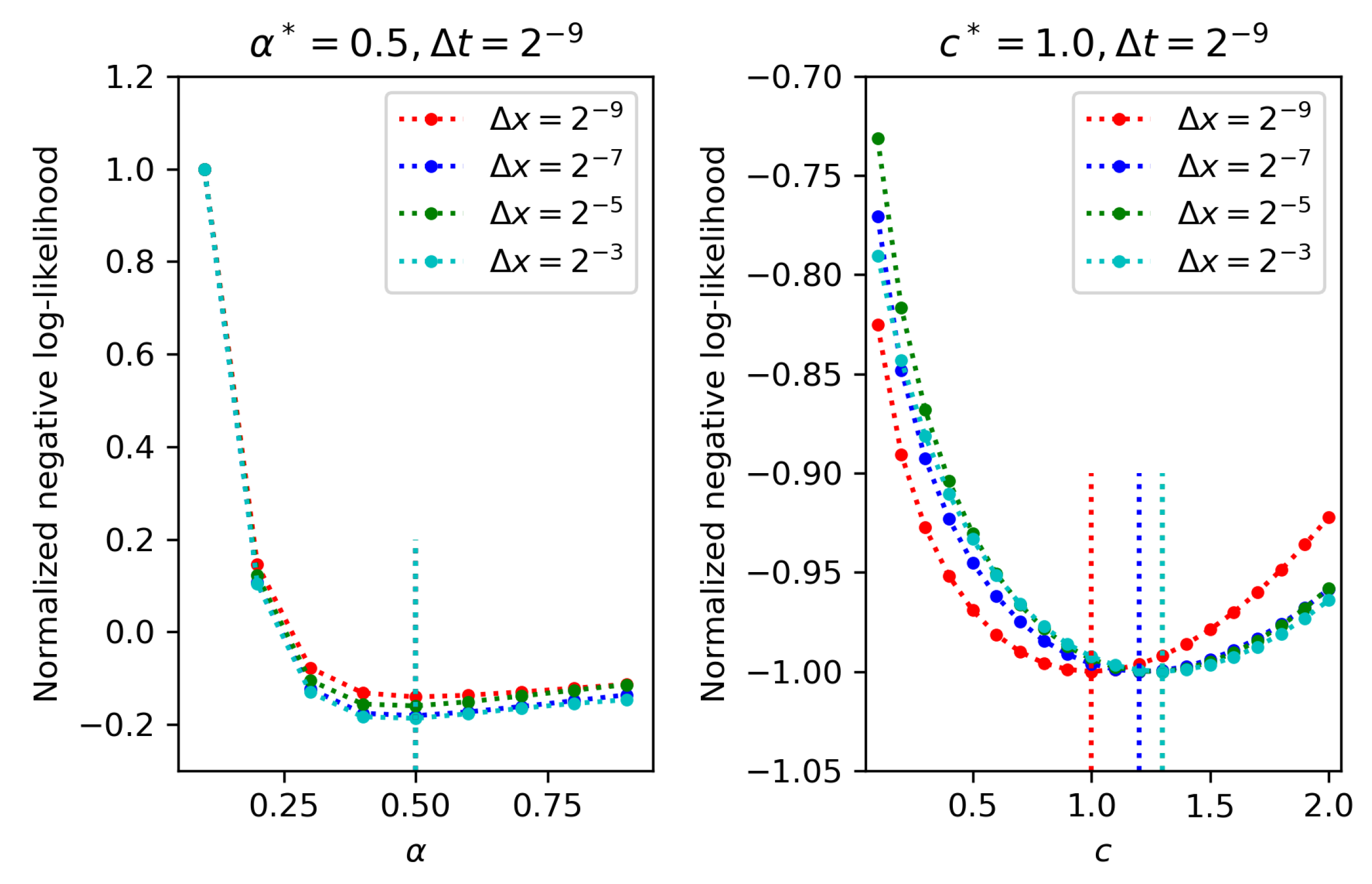
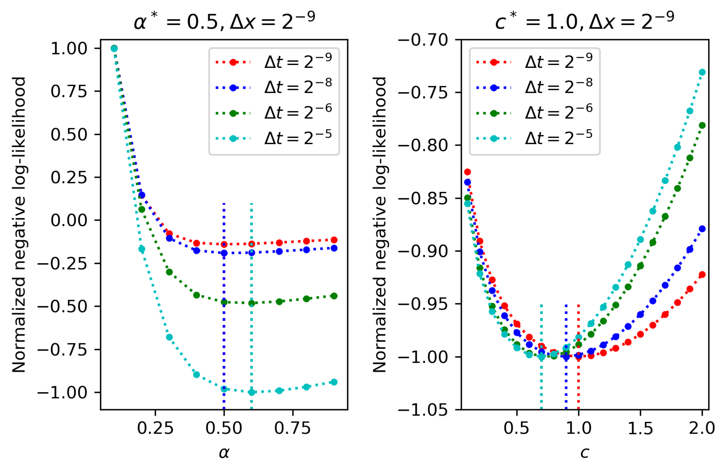
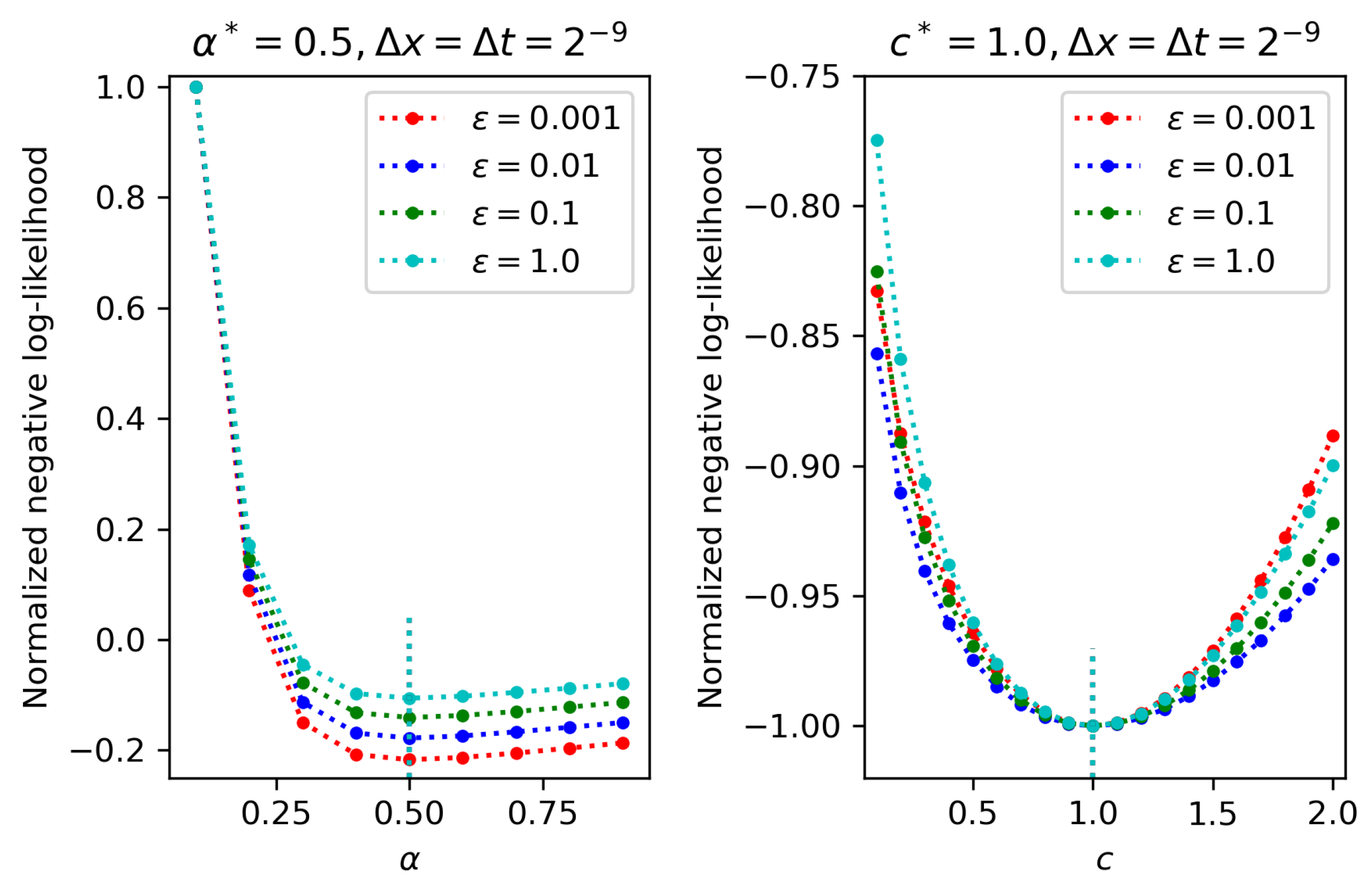
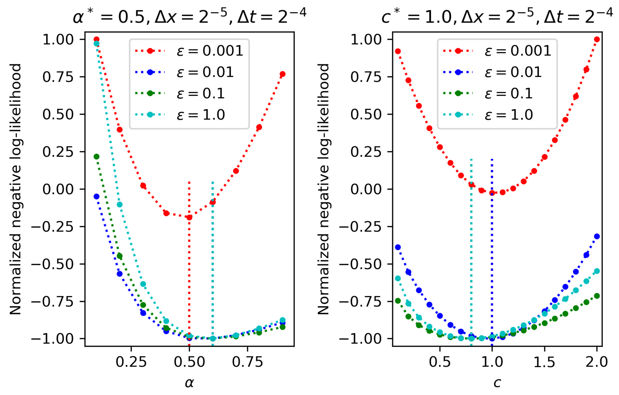
4.1. One-Parameter Estimation

We first consider the full observation ${\overline{U}}_{2^{-9},2^{-9}}$ shown in the right panel of Figure 1, which corresponds to the noise sample point ${\omega }^0$. We plot the exact negative log-likelihood function −$log\tilde{L}(\alpha ,c,ϵ)$ by varying one of the three parameters $(\alpha ,c,ϵ)$ but fixing the other two to their true values. In the left panel of Figure 3, we plot a red dotted line corresponding to $-log\tilde{L}(\alpha ,c^{*},{ϵ}^{*})$ for $\alpha =0.1,0.2,\cdots ,0.9$ and ${\Delta }_{0}x={\Delta }_{0}t=2^{-9}$. We see that the optimal $\alpha$ that minimizes the negative log-likelihood is 0.5, and it agrees with the true ${\alpha }^{*}=0.5$. Now, we consider the partial observation by increasing the spatial step ${\Delta }_{0}x$ to $4{\Delta }_{0}x,16{\Delta }_{0}x$, and $64{\Delta }_{0}x$, and we plot the corresponding exact negative log-likelihoods with blue, green, and cyan dotted lines. The optimal $\alpha$ does not alter with increasing $\Delta x$. This indicates that the spatial step does not affect too much the estimation of $\alpha$ when other two parameters are fixed to their true values. This is not the case for estimating c, however. In the right panel of Figure 3, the optimal c also matches the true value $c^{*}=1$ for the full observation case, whereas the optimal c’s for partial observation cases begin to shift to the right of the true value. Furthermore, the larger the spatial step is, the more the optimal c shifts to the right. This implies that the estimation of c is more sensitive to increasing spatial step than the estimation of $\alpha$.

We have considered the effect of spatial step on the optimal $\alpha$ and c for fixed temporal step. We next consider the opposite, namely, the effect of temporal step for fixed spatial step. From Figure 4, we see that estimations of $\alpha$ and c are both sensitive to the varying temporal steps. This suggests that when recording the concentration data using sensors we can place a small number of sensors in space but we must ensure that the data can be recorded with high sampling frequency in time.

We last consider the sensitivity of estimated $\alpha$ and c to the magnitude of noise $ϵ$. We see from Figure 5 that for a full observation the noise magnitude has no impact on the optimal $\alpha$ and c. In contrast, Figure 6 illustrates that for the partial observation with $r_x=16$ and $r_t=32$ the optimal $\alpha$ and c can differ from their true values; moreover, the larger the noise is, the more likely the shift occurs.

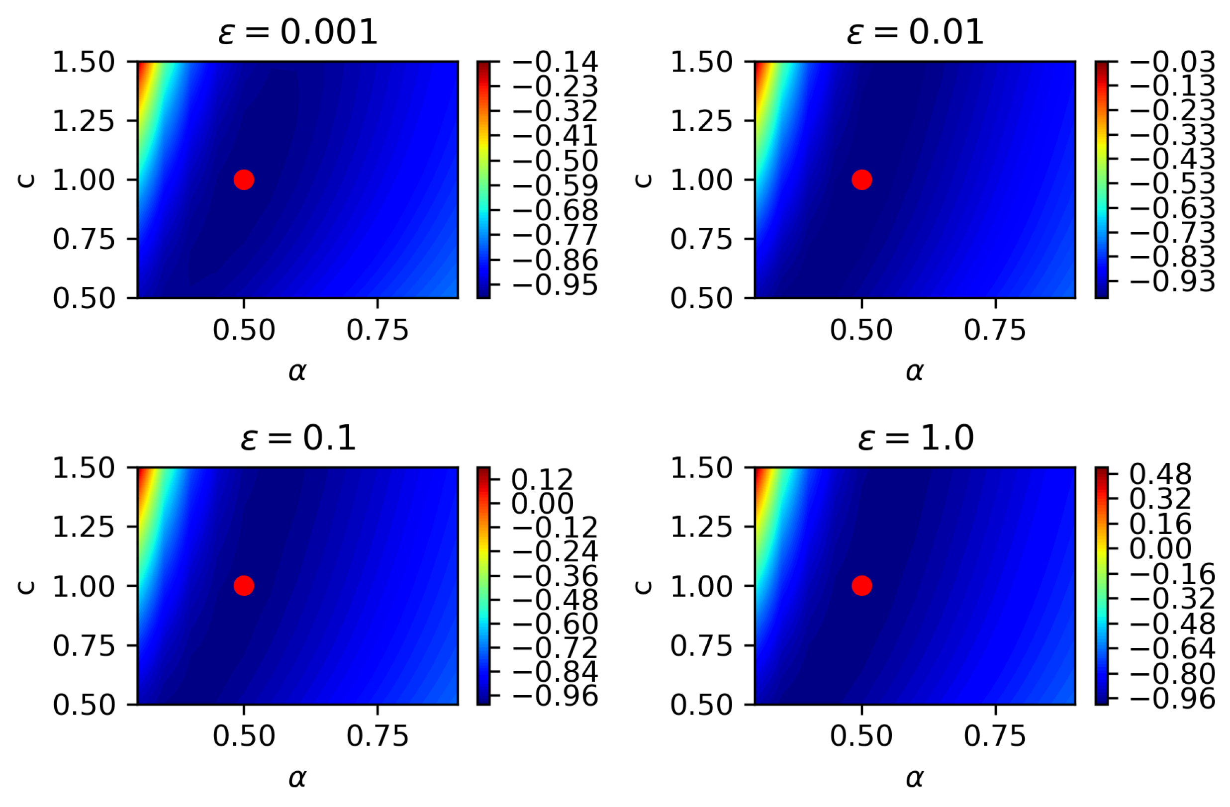
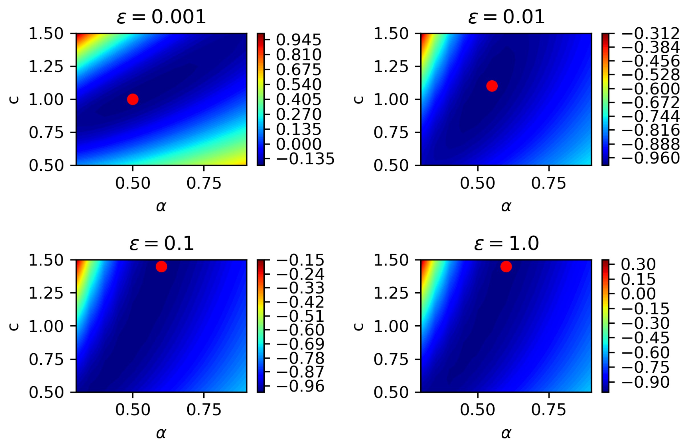
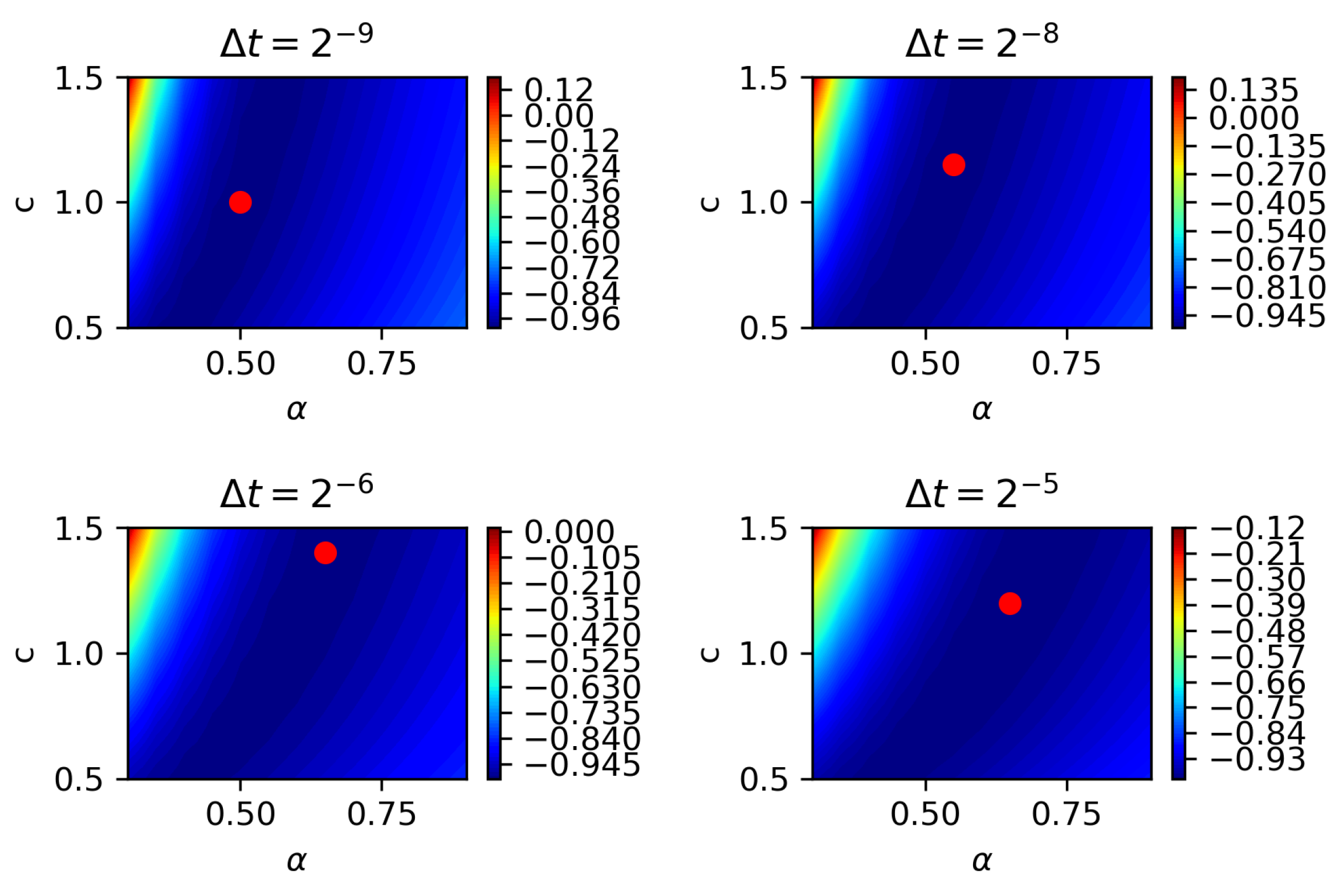
4.2. Two-Parameter Estimation

We now estimate jointly parameters $\alpha$ and c from the full observation shown in the right panel of Figure 1. In first case, we fix the temporal step to ${\Delta }_{0}t=2^{-9}$ and change the spatial step. Figure 7 plots how the optimal $(\alpha ,c)$ (the red disk in the figure) alters its position in the contour plot when the spatial step varies. We see that for a full observation, the optimal parameters can always match the true parameters, whereas for partial observations, the diffusion coefficient c is more difficult to be estimated than the fractional order $\alpha$. In second case, we fix the spatial step to ${\Delta }_{0}x=2^{-9}$ but change the temporal step. From Figure 8 we see that increasing the temporal step makes both the optimal $\alpha$ and c deviate from their true values, which implies, just as in the one-parameter estimation case, that a small temporal step is preferred to a small spatial step when high accuracy of partial observation is expected. In third case, we fix spatio-temporal steps while varying the noise magnitude $ϵ$. In Figure 9, we fix the spatio-temporal steps to be $r_x=r_t=1$ (a full observation), and we see that the magnitude of noise does not affect the optimal parameters; this is the same as in the case of one-parameter estimation. In Figure 10, we consider a partial observation by setting the sampling ratios to $r_x=16$ and $r_t=8$, and we observe that the larger the noise magnitude is, the more the optimal parameters deviate from the true parameters.

So far, we have estimated parameters using a trial-and-error approach. Specifically, we computed the exact negative log-likelihood for all parameters on a uniform grid in the parameter space and then selected the optimal parameter among the parameters on this grid. Sometimes, however, the true parameter, say, ${\alpha }^{*}=0.345$, is located on a rather dense grid, and employing the trial-and-error approach could be time-consuming. We next utilize certain optimization algorithm to find the optimal parameters. In this paper, we employ a type of quasi-Newton method, called L-BFGS-B algorithm [26] to minimize the negative log-likelihood $-log\tilde{L}(\alpha ,c,ϵ)$. To implement the algorithm, we adopt the optimization algorithm package provided in SciPy (see scipy.optimization.minimize()), and set the optional parameters in the algorithm routine to their default values.

As different full observations will yield different estimates of parameters, we consider 20 different full observations obtained by solving the forward problems under different sample-points of noise: ${\omega }^k$ for $k=0,1,\cdots ,19$. In

Table 1. Two-parameter estimation: Mean of the estimated $(\alpha ,c)$ from 20 different full observations. The effect of sparsity of observation (i.e., sampling rations $r_x$ and $r_t$) on the mean of the estimated parameters is demonstrated. The true parameters are ${\alpha }^{*}=0.5$ and $c^{*}=1$. The noise magnitude is fixed to ${ϵ}^{*}=0.1$. A quasi-Newton optimization algorithm, L-BFGS-B algorithm, is employed to minimize the negative log-likelihood.

Mean $\widehat{\mathit{\alpha }}$	${\mathit{r}}_{\mathit{x}}=128$	64	32	16	8	4	2	1
$r_t=32$	0.673	0.634	0.649	0.664	0.673	0.682	0.682	0.683
$r_t=16$	0.621	0.603	0.612	0.628	0.637	0.645	0.648	0.651
$r_t=8$	0.581	0.573	0.589	0.603	0.611	0.617	0.620	0.621
$r_t=4$	0.555	0.557	0.569	0.579	0.582	0.586	0.588	0.590
$r_t=2$	0.528	0.26	0.536	0.544	0.546	0.548	0.550	0.551
$r_t=1$	0.491	0.485	0.492	0.497	0.498	0.499	0.500	0.500
Mean$\widehat{\mathit{c}}$	${\mathit{r}}_{\mathit{x}}=\mathbf{128}$	64	32	16	8	4	2	1
$r_t=32$	1.455	1.259	1.277	1.307	1.314	1.324	1.264	1.100
$r_t=16$	1.428	1.297	1.317	1.365	1.386	1.400	1.351	1.183
$r_t=8$	1.409	1.316	1.379	1.438	1.466	1.478	1.423	1.238
$r_t=4$	1.400	1.371	1.424	1.473	1.485	1.487	1.432	1.248
$r_t=2$	1.361	1.326	1.375	1.410	1.411	1.408	1.355	1.177
$r_t=1$	1.233	1.186	1.211	1.223	1.219	1.205	1.155	1.000

, we show the mean values of 20 pairs of parameters $(\widehat{\alpha }\left({\omega }^k\right),\widehat{c}\left({\omega }^k\right))$ where we put the noise sample point ${\omega }^k$ in the parentheses behind each parameter to emphasize the dependency of parameter on sample point.

Table 2. Two-parameter estimation: Standard deviation (std) of the estimated $(\alpha ,c)$ from 20 different full observations. The effect of sparsity of observation on the std of the estimated parameters is demonstrated. The noise magnitude is fixed to ${ϵ}^{*}=0.1$.

Std $\widehat{\mathit{\alpha }}$	${\mathit{r}}_{\mathit{x}}=128$	64	32	16	8	4	2	1
$r_t=32$	0.094	0.062	0.044	0.032	0.023	0.019	0.014	0.009
$r_t=16$	0.071	0.045	0.035	0.025	0.016	0.012	0.009	0.007
$r_t=8$	0.056	0.033	0.024	0.017	0.013	0.010	0.007	0.005
$r_t=4$	0.035	0.023	0.016	0.011	0.007	0.006	0.004	0.003
$r_t=2$	0.027	0.017	0.011	0.008	0.007	0.005	0.003	0.002
$r_t=1$	0.021	0.010	0.007	0.006	0.005	0.004	0.003	0.002
Std$\widehat{\mathit{c}}$	${\mathit{r}}_{\mathit{x}}=\mathbf{128}$	64	32	16	8	4	2	1
$r_t=32$	0.392	0.225	0.167	0.121	0.088	0.072	0.049	0.278
$r_t=16$	0.350	0.211	0.173	0.123	0.077	0.062	0.045	0.028
$r_t=8$	0.327	0.182	0.140	0.102	0.081	0.066	0.046	0.027
$r_t=4$	0.254	0.151	0.112	0.080	0.060	0.050	0.032	0.020
$r_t=2$	0.215	0.122	0.084	0.065	0.055	0.038	0.027	0.015
$r_t=1$	0.161	0.075	0.054	0.046	0.041	0.028	0.019	0.011

displays the standard deviation of these 20 pairs of parameters.

From Table 1, we see that keeping $r_t$ small yields more accurate estimates than keeping $r_x$ small, which accords with our comment for Figure 8. Moreover, a full observation with $r_x=r_t=1$, again, achieves the highest accuracy for parameter estimation, which validates our approach. From Table 2 we can see that the standard deviation of diffusion coefficient is obviously larger than that of fractional order, and this implies that the former is more difficult to be estimated than the latter. This implication matches our observation for the one-parameter estimation case. Additionally, we see from Table 2 that the more accurate the mean of estimates is, the smaller the standard deviation of estimates is. This gives a suggestion that when we do not know the true parameters we can judge if the estimated parameters are reliable by checking the magnitude of standard deviation.

4.3. Three-Parameter Estimation

Table 3. Three-parameter estimation: Estimated $(\alpha ,c,ϵ)$ from the full observation shown in the right panel of Figure 1. The effect of sparsity of observation on estimated parameters is demonstrated. The true parameters are ${\alpha }^{*}=0.5,c^{*}=1$, and ${ϵ}^{*}=0.1$. A quasi-Newton optimization algorithm, L-BFGS-B algorithm is employed to minimize the negative log-likelihood.

$\widehat{\mathit{\alpha }}$	${\mathit{r}}_{\mathit{x}}=128$	64	32	16	8	4	2	1
$r_t=32$	0.495	0.596	0.661	0.668	0.665	0.694	0.683	0.691
$r_t=16$	0.518	0.583	0.609	0.607	0.614	0.650	0.651	0.662
$r_t=8$	0.518	0.558	0.576	0.586	0.597	0.624	0.627	0.632
$r_t=4$	0.505	0.515	0.548	0.565	0.569	0.586	0.587	0.590
$r_t=2$	0.498	0.497	0.512	0.533	0.536	0.547	0.549	0.553
$r_t=1$	0.456	0.456	0.473	0.487	0.491	0.496	0.500	0.500
$\widehat{\mathit{c}}$	${\mathit{r}}_{\mathit{x}}=\mathbf{128}$	64	32	16	8	4	2	1
$r_t=32$	1.382	1.152	1.137	1.170	1.162	1.174	1.155	1.101
$r_t=16$	1.281	1.192	1.190	1.252	1.246	1.260	1.217	1.096
$r_t=8$	1.246	1.211	1.272	1.378	1.391	1.376	1.448	1.079
$r_t=4$	1.720	1.686	1.845	2.000	1.980	1.950	1.496	1.360
$r_t=2$	1.5000	1.554	1.726	1.880	1.862	1.857	1.441	1.337
$r_t=1$	1.369	1.463	1.622	1.744	1.730	1.709	1.523	1.038
$\widehat{\mathbf{ϵ}}$	${\mathit{r}}_{\mathit{x}}=\mathbf{128}$	64	32	16	8	4	2	1
$r_t=32$	0.162	0.109	0.091	0.091	0.093	0.085	0.091	0.098
$r_t=16$	0.130	0.102	0.094	0.078	0.096	0.087	0.088	0.089
$r_t=8$	0.109	0.099	0.098	0.101	0.100	0.090	0.099	0.084
$r_t=4$	0.146	0.146	0.141	0.142	0.140	0.131	0.105	0.108
$r_t=2$	0.122	0.132	0.139	0.139	0.138	0.132	0.107	0.112
$r_t=1$	0.126	0.140	0.146	0.148	0.147	0.143	0.131	0.104

gives the estimated parameters from the full observation shown in the right panel of Figure 1. The initial guess for the three parameters in the L-BFGS-B algorithm is $({\alpha }_0,c_0,{ϵ}_0)=(0.8,0.5,0.5)$ while the true parameters are $({\alpha }^{*},c^{*},{ϵ}^{*})=(0.5,1.0,0.1)$. Like the one-parameter and two-parameter estimation cases, the full observation case ($r_x=r_t=1)$ again achieves highest estimation accuracy. Jointly estimating three parameters from a partial observation, however, could not be reliable, even though $r_t$ and $r_x$ are both small. For example, for $r_t=1$ and $r_x=2$, the estimated diffusion coefficient is 1.523, while the true parameter is only 1.0. This indicates that for this case, we need to approach a full observation by keeping the spatio-temporal steps as small as possible so as to attain high estimation accuracy. Among the three parameters that are estimated, the diffusion coefficient is again most difficult to be estimated. This agrees with our observation for the one-parameter and two-parameter estimation cases.

We next consider the effect of true fractional order on the parameter estimation. We have fixed the true fractional order to ${\alpha }^{*}=0.5$ so far, but now we will see if we can still recover parameters when ${\alpha }^{*}$ is changed. We freeze the spatial-temporal steps to ${\Delta }_{0}x={\Delta }_{0}t=2^{-9}$, fix the sample point to ${\omega }^0$ as before, but generate the full observations ${\overline{U}}_{{\Delta }_{0}x,{\Delta }_{0}t}^{0.1}$ and ${\overline{U}}_{{\Delta }_{0}x,{\Delta }_{0}t}^{0.9}$ using ${\alpha }^{*}=0.1$ and ${\alpha }^{*}=0.9$, respectively, where the superscript of $\overline{U}$ represents the dependency on the true fractional order. We have seen from Table 3 that the estimated parameters for ${\overline{U}}_{{\Delta }_{0}x,{\Delta }_{0}t}^{0.5}$ are $(\widehat{\alpha },\widehat{c},\widehat{ϵ})=(0.500,1.038,0.104)$. We observe that the estimated parameters for other two full observations are sufficiently accurate as well, i.e., $(\widehat{\alpha },\widehat{c},\widehat{ϵ})=(0.100,1.035,0.104)$ for ${\overline{U}}_{{\Delta }_{0}x,{\Delta }_{0}t}^{0.1}$ and $(\widehat{\alpha },\widehat{c},\widehat{ϵ})=(0.900,1.002,0.100)$ for ${\overline{U}}_{{\Delta }_{0}x,{\Delta }_{0}t}^{0.9}$. We need to point out that for smaller ${\alpha }^{*}$, say, 0.1 here, the negative log-likelihood appears to be flatter in the neighborhood of global minimizer ${\alpha }^{*}=0.1$, compared with a large ${\alpha }^{*}$, say 0.5. For example, for ${\overline{U}}_{{\Delta }_{0}x,{\Delta }_{0}t}^{0.1}$, the negative log-likelihood for the parameter triple $(0.0999,1.528,0.1526)$ is approximately −3,335,910, while the negative-likelihood for true parameters $(0.1,1.0,0.1)$ is approximately −3,335,916. In the neighborhood of true parameters, the negative log-likelihood can only change $\frac{|3,335,916-3,335,910|}{3,335,916}\approx 0.0002\%$. This minor variation could challenge the optimization algorithms. For the L-BFGS-B algorithm, if we set the iteration termination tolerances ftol and gtol to larger values, say, the default values ftol = 1e-9 and gtol = 1e-5, we arrive to the aforementioned parameters $(0.0999,1.528,0.1526)$. By resetting ftol = 1e-12 and gtol = 1e-9, we obtain much better estimates $(0.100,1.035,0.104)$. Note that for parameter estimation in other two full observations, we still use the default tolerances for sake of computational cost.

On the other hand, the negative log-likelihood can also become flatter near the global minimizer when the final observation time decreases. The final observation time we previously consider is $T=1$, but now we reset it to $T=1/4$ and $T=1/16$, with spatio-temporal steps and noise sample point fixed as before. The true fractional order is taken to 0.5. We first consider the case of default ftol and gtol. For $T=1/4$, the estimated parameters are $(0.5008,1.0932,0.1088)$, whose accuracy is acceptable, whereas for $T=1/16$, the estimated parameters are $(0.4978,1.3775,0.1387)$, which is not that accurate. Now we switch to ftol = 1e-12 and gtol = 1e-9, and see that the estimated parameters for $T=1/4$ do not change, but those for $T=1/16$ become much better ones $(0.4962,1.0268,0.1045)$. Therefore, for a small final observation time, it is safe to keep using small iteration termination tolerances.

Here are some comments on time complexity in implementing the pseudo-likelihood approach proposed in the paper. The time complexity is

$$M\left[O\left({\left(\frac{N_{0x}}{r_x}\right)}^2{\left(\frac{N_{0t}}{r_t}\right)}^2\right)+O\left({\left(\frac{N_{0x}}{r_x}\right)}^3\right)\right],$$

(34)

where M is the number of evaluations of negative log-likelihood function in the L-BFGS-B algorithm. The number M is affected by the number of parameters to be estimated (or the dimensionality of parameter space) and the iteration termination tolerances aforementioned. For example, for a full observation with default tolerances, a two-parameter estimation requires $M=45$, while a three-parameter estimation with the default tolerances requires $M=140$. The term ${(N_{0t}/r_t)}^2$ comes from the time discretization of fractional time derivative ${\partial }_t^{1-\alpha }\mathbf{A}\overline{\mathbf{U}}\left(t\right)$, and ${(N_{0x}/r_x)}^2$ arises from the multiplication of difference matrix $\mathbf{A}$ and observation vector ${\overline{\mathbf{U}}}^n$. The last term ${(N_{0x}/r_x)}^3$ appears due to the inversion of and Cholesky decomposition of $\mathbf{B}$. In our computational experiment, it took 7523 seconds to estimate $(\alpha ,c,ϵ)$ for the full observation case (${\omega }^0)$, in which $M=140,N_{0x}=N_{0t}=512$, and $r_x=r_t=1$. The code was run at a laptop workstation with Intel(R) Core(TM) i7-10850H CPU @ 2.70GHz and 64 GB memory.

We provide at Github (The code examples can be downloaded at https://github.com/Derek2021Pang/pseudo_likelihood_SFPDE) two Python code examples. The first example is a forword solver, which can generate full observation for given spatio-temporal steps and white noise sample, and the second example is a pseudo-likelihood parameter estimator, which can estimate the parameters from the full observation by employing the L-BFGS-B algorithm.

5. Concluding Remarks

In the paper, we propose a pseudo-likelihood approach to estimating the parameters of a one-dimensional stochastic time-fractional diffusion problem (2). We consider full observation and partial observation cases when different amounts of information are available. For the full observation case, our approach can accurately estimate equation (or model) parameters for one-parameter, two-parameter, and three-parameter estimation problems. For the partial observation case, the accuracy of estimated parameters are affected by the sparsity of the observation data, which is controlled by the spatio-temporal sampling steps $\Delta x$ and $\Delta t$ (or $r_x$ and $r_t$). Our computational experiments produce the following observations:

i

The larger the spatio-temporal sampling steps are, the lower the accuracy of estimated parameters is, which is intuitive.

ii

Keeping temporal sampling step small is more important than keeping spatial step small in terms of increasing the parameter estimation accuracy for partial observation.

iii

Among the three parameters being estimated, namely, fractional order, diffusion coefficient, and noise magnitude, the diffusion coefficient is most difficult to be estimated, since it is most sensitive to varying spatio-temporal steps in partial observation.

iv

The high accuracy of mean of estimated parameters is usually related to the low standard deviation of estimated parameters, when we fortunately have multiple observations, corresponding to different realizations of driving noise, to obtain multiple groups of estimated parameters.

v

Estimating more parameters jointly leads to larger variability of estimated parameters when spatio-temporal steps increase. Making spatio-temporal steps as small as possible is suggested for a joint estimation of a large number of parameters.

We need to point out, however, that a limitation of the current approach is that the observed data must be distributed at a uniform grid in the space and time. Otherwise, we cannot compute the negative-likelihood function using the finite difference schemes in the forward solver. The approach cannot handle the case where scattered observation data is present.

In reality, when confronted by discrete observation data, we need to pay attention to three points: First, we do not know in advance whether or not the observation is a full observation. The judgment largely depends on what equation model we consider, what discretization scheme we adopt, and what spatial-temporal steps we take. As we have pointed out, when one already chooses the right model and right discretization, one could make a good parameter estimation if the observation data is dense in time but sparse in space. Second, we may take into account model selection problem when we do not have preference for a specific model but have several candidate models. To select a good model, we can consider a scoring strategy. We score each candidate model with the minimum of the corresponding negative log-likelihood and choose the model having the lowest score. Third, different discretization schemes will lead to different pseudo-likelihood function $\tilde{L}(·)$. Thus, it could be sensible for a given model to select a discretization scheme that yields a pseudo-likelihood estimation more robust to spatial-temporal sampling steps.

Unlike the maximum likelihood estimators presented in [8,11], we do not make any theoretical analyses on asymptotic properties of our pseudo-likelihood estimators. This is one of our future works. It is straightforward to extend the current pseudo-likelihood approach to two- and three-dimensional problems. However, extending the approach to other types of equations, such as space-time fractional stochastic PDEs (1) and even the stochastic versions of variable-order fractional PDEs [27,28], is not that trivial. Reliable discretization schemes for target equations are needed to be developed for those equations, and proper parametrization is required for the variable fractional orders. Furthermore, we will consider in the future the parameter estimation for fractional diffusion equations perturbed by fractional Brownian motion and Lévy motion.

References

1. Mijena, J.B.; Nane, E. Space–time fractional stochastic partial differential equations. J. Stoch. Process Their Appl. 2015, 125, 3301–3326. [Google Scholar] [CrossRef]
2. Anh, V.V.; Leonenko, N.N.; Ruiz-Medina, M.D. Fractional-in-time and multifractional-in-space stochastic partial differential equations. Fract. Calc. Appl. Anal. 2016, 19, 1434–1459. [Google Scholar] [CrossRef] [Green Version]
3. Gunzburger, M.; Li, B.Y.; Wang, J.L. Sharp convergence rates of time discretization for stochastic time-fractional PDEs subject to additive space-time white noise. Math. Comput. 2019, 88, 1715–1741. [Google Scholar] [CrossRef]
4. Bolin, D.; Kirchner, K.; Kovács, M. Fractional-in-time and multifractional-in-space stochastic partial differential equations. IMA J. Numer. Anal. 2020, 40, 1051–1073. [Google Scholar] [CrossRef]
5. Anh, V.V.; Olenko, A.; Wang, Y.G. Fractional stochastic partial differential equation for random tangent fields on the sphere. arXiv 2021, arXiv:2107.03717. [Google Scholar]
6. Mohammed, W.W. Approximate solutions for stochastic time-fractional reaction–diffusion equations with multiplicative noise. Math. Methods Appl. Sci. 2021, 44, 2140–2157. [Google Scholar] [CrossRef]
7. Xia, D.F.; Yan, L.T. Some properties of the solution to fractional heat equation with a fractional Brownian noise. Adv. Differ. Equ. 2017, 107, 1–16. [Google Scholar] [CrossRef] [Green Version]
8. Huebner, M.; Rozovskii, B.L. AOn asymptotic properties of maximum likelihood estimators for parabolic stochastic PDE’s. Probab. Theory Relat. Fields 1995, 103, 143–163. [Google Scholar] [CrossRef]
9. Bishwal, J.P.N. Parameter Estimation in Stochastic Differential Equations; Springer: Berlin/Heidelberg, Germany, 2007. [Google Scholar]
10. Rao, B.L.S.P. Statistical Inference for Fractional Diffusion Processes; John Wiley & Sons: Hoboken, NJ, USA, 2011. [Google Scholar]
11. Huebner, M.; Khasminskii, R.; Rozovskii, B.L. Two examples of parameter estimation for stochastic partial differential equations. In Stochastic Processes: A Festschrift in Honour of Gopinath Kallianpur; Cambanis, S., Ghosh, J.K., Karandikar, R.L., Sen, P.K., Eds.; Springer: New York, NY, USA, 1993; pp. 149–160. [Google Scholar]
12. Cialenco, I.; Lototsky, S.V.; Pospíšil, J. Asymptotic properties of the maximum likelihood estimator for stochastic parabolic equations with additive fractional Brownian motion. Stoch. Dyn. 2009, 9, 169–185. [Google Scholar] [CrossRef]
13. Cialenco, I. Parameter estimation for SPDEs with multiplicative fractional noise. Stoch. Dyn. 2010, 10, 561–576. [Google Scholar] [CrossRef]
14. Geldhauser, C.; Valdinoci, E. Optimizing the fractional power in a model with stochastic PDE constraints. Adv. Nonlinear Stud. 2018, 18, 649–669. [Google Scholar] [CrossRef] [Green Version]
15. Aster, R.C.; Borchers, B.; Thurber, C.H. Parameter Estimation and Inverse Problems; Elsevier: Amsterdam, The Netherlands, 2005. [Google Scholar]
16. Pang, G.F.; Perdikaris, P.; Cai, W.; Karniadakis, G.E. Discovering variable fractional orders of advection–dispersion equations from field data using multi-fidelity Bayesian optimization. J. Comput. 2017, 348, 694–714. [Google Scholar] [CrossRef]
17. Yan, L.; Guo, L. Stochastic Collocation Algorithms Using l1-Minimization for Bayesian Solution of Inverse Problems. SIAM J. Sci. Comput. 2015, 37, A1410–A1435. [Google Scholar] [CrossRef]
18. Garcia, L.A.; Shigidi, A. Using neural networks for parameter estimation in ground water. J. Hydrol. 2006, 318, 215–231. [Google Scholar] [CrossRef]
19. Pang, G.F.; Lu, L.; Karniadakis, G.E. fPINNs: Fractional physics-informed neural networks. SIAM J. Sci. Comput. 2019, 41, A2603–A2626. [Google Scholar] [CrossRef]
20. Da, P.G.; Zabczyk, J. Stochastic Equations in Infinite Dimensions; Cambridge University Press: Cambridge, UK, 2014. [Google Scholar]
21. Kilbas, A.A.; Srivastava, H.M.; Trujillo, J.J. Theory and Applications of Fractional Differential Equations; Elsevier: Amsterdam, The Netherlands, 2006. [Google Scholar]
22. Iacus, S.M. Simulation and Inference for Stochastic Differential Equations: With R Examples; Springer: Berlin/Heidelberg, Germany, 2009. [Google Scholar]
23. Yoshida, N. Estimation for diffusion processes from discrete observation. J. Multivar. Anal. 1992, 41, 220–242. [Google Scholar] [CrossRef] [Green Version]
24. Lubich, C. Convolution quadrature and discretized operational calculus. I. Numer. Math. 1988, 52, 129–145. [Google Scholar] [CrossRef]
25. Lubich, C. Convolution quadrature and discretized operational calculus. II. Numer. Math. 1988, 52, 413–425. [Google Scholar] [CrossRef]
26. Byrd, R.H.; Lu, P.H.; Nocedal, J.; Zhu, C.Y. A limited memory algorithm for bound constrained optimization. SIAM J. Sci. Comput. 1995, 16, 1190–1208. [Google Scholar] [CrossRef]
27. Zheng, X.C.; Wang, H. An error estimate of a numerical approximation to a hidden-memory variable-order space-time fractional diffusion equation. SIAM J. Numer. Anal. 2020, 58, 2492–2514. [Google Scholar] [CrossRef]
28. Zheng, X.C.; Wang, H. Wellposedness and regularity of a variable-order space-time fractional diffusion equation. Anal. Appl. 2020, 18, 615–638. [Google Scholar] [CrossRef]
29. Hogg, R.V.; McKean, J.; Craig, A.T. Introduction to Mathematical Statistics; Pearson Education: London, UK, 2005. [Google Scholar]
Figure 1. Full observations with Δ 0 x = Δ 0 t = 2 9 for noise magnitude ϵ = 0 (left panel) and ϵ = 0.1 (right panel). The fractional order and diffusion coefficient are fixed to α * = 0.5 and c * = 1.0 , respectively.
Fractalfract 05 00129 g001
Figure 2. The realization of the noise term Z ( ω 0 ) in (18) that yields the full observation in the right panel of Figure 1. The noise magnitude is set to ϵ * = 0.1 .
Fractalfract 05 00129 g002
Figure 3. One-parameter estimation: Negative log-likelihood curves for varying α [ 0.1 , 0.9 ] and fixed c * = 1.0 (left) and for varying c [ 0.1 , 2 ] and fixed α * = 0.5 (right). The effect of spatial step on the optimal parameters is demonstrated. The noise magnitude is fixed to ϵ * = 0.1 . Full observation and partial observation curves are displayed in different colors. As these curves have y values with several orders of magnitude, for convenience of comparison, the y values are normalized by dividing the y values of each curve by their maximum absolute values. The temporal step is fixed to that of full observation, i.e., Δ 0 t = 2 9 ; the spatial steps vary, and Δ x = 2 9 corresponds to the full observation case, while the other three spatial steps correspond to the partial observation cases with r x = 4 , 16 , and 64. The vertical dotted lines intersect x-axis at the optimal α or c that minimizes the normalized negative log-likelihood. The optimal parameters are regarded as the estimated parameters. Note that a vertical line having a specific color corresponds to the likelihood curve having the same color, and vertical lines can overlap each other when the optimal parameters are the same.
Fractalfract 05 00129 g003
Figure 4. One-parameter estimation: Negative log-likelihood curves for varying α and fixed c * = 1.0 (left) and for varying c and fixed α * = 0.5 (right). The effect of temporal step on the optimal parameters is demonstrated. The noise magnitude is fixed to ϵ * = 0.1 . Full observation and partial observation curves are displayed in different colors. The spatial step is fixed to that of full observation, i.e., Δ 0 x = 2 9 ; the temporal steps vary, and Δ t = 2 9 corresponds to the full observation case, while the other three spatial steps correspond to partial observation cases with r t = 2 , 8 , and 16.
Fractalfract 05 00129 g004
Figure 5. One-parameter estimation for a full observation: Negative log-likelihood curves for varying α and fixed c * = 1.0 (left) and for varying c and fixed α * = 0.5 (right). The effect of noise magnitude on the optimal parameters is demonstrated. Curves for different noise magnitudes are displayed in different colors. The spatio-temporal steps are fixed to those of a full observation, i.e., Δ 0 t = Δ 0 x = 2 9 .
Fractalfract 05 00129 g005
Figure 6. One-parameter estimation for a partial observation: Negative log-likelihood curves for varying α and fixed c * = 1.0 (left) and for varying c and fixed α * = 0.5 (right). The effect of noise magnitude on the optimal parameters is demonstrated. Curves for different noise magnitudes are displayed in different colors. The spatio-temporal steps are fixed to those of a specific partial observation with r x = 16 and r t = 32 .
Fractalfract 05 00129 g006
Figure 7. Two-parameter estimation: Contour plots of normalized negative log-likelihood for pairs of ( α , c ) [ 0.3 , 0.9 ] × [ 0.5 , 1.5 ] . The effect of spatio step on the estimated parameters is demonstrated. The noise magnitude is taken to its true value ϵ * = 0.1 . The true values for α and c are α * = 0.5 and c * = 1.0 . The full observation case r x = 1 is compared with other three partial observation cases with r x = 4 , 16 , and 64. For all plots, the other controlling parameter for partial observation is fixed to r t = 1 . The red disk represents the optimal parameter pair that minimizes the negative log-likelihood.
Fractalfract 05 00129 g007
Figure 8. Two-parameter estimation: Contour plots of normalized negative log-likelihood for pairs of ( α , c ) [ 0.3 , 0.9 ] × [ 0.5 , 1.5 ] . The effect of temporal step on the estimated parameters is demonstrated. The noise magnitude is taken to its true value ϵ * = 0.1 . The true values for α and c are α * = 0.5 and c * = 1.0 . The full observation case r t = 1 is compared with other three partial observation cases with r t = 2 , 8 , and 32. For all plots, the other controlling parameter for partial observation is fixed to r x = 1 . The red disk represents the optimal parameter pair that minimize the negative log-likelihood.
Fractalfract 05 00129 g008
Figure 9. Two-parameter estimation for a full observation: Contour plots of normalized negative log-likelihood for pairs of ( α , c ) [ 0.3 , 0.9 ] × [ 0.5 , 1.5 ] . The effect of noise magnitude on the estimated parameters is demonstrated. The true values for α and c are α * = 0.5 and c * = 1.0 . The plots for different noise magnitudes are compared. For all plots, the controlling parameters for partial observation are fixed to r x = r t = 1 (namely, a full observation). The red disk represents the optimal parameter pair that minimizes the negative log-likelihood.
Fractalfract 05 00129 g009
Figure 10. Two-parameter estimation for a partial observation: Contour plots of normalized negative log-likelihood for pairs of ( α , c ) [ 0.3 , 0.9 ] × [ 0.5 , 1.5 ] . The effect of noise magnitude on the estimated parameters is demonstrated. The true values for α and c are α * = 0.5 and c * = 1.0 . The plots for different noise magnitudes are compared. For all plots, the controlling parameters for partial observation are fixed to r x = 16 and r t = 8 . The red disk represents the optimal parameter pair that minimizes the negative log-likelihood.
Fractalfract 05 00129 g010