Analytic Solution of the Langevin Differential Equations Dominated by a Multibrot Fractal Set

Abstract

We present an analytic solvability of a class of Langevin differential equations (LDEs) in the asset of geometric function theory. The analytic solutions of the LDEs are presented by utilizing a special kind of fractal function in a complex domain, linked with the subordination theory. The fractal functions are suggested for the multi-parametric coefficients type motorboat fractal set. We obtain different formulas of fractal analytic solutions of LDEs. Moreover, we determine the maximum value of the fractal coefficients to obtain the optimal solution. Through the subordination inequality, we determined the upper boundary determination of a class of fractal functions holding multibrot function $\vartheta \left(z\right)=1+3\kappa z+z^3$.

1. Introduction

The class of Langevin differential equations (LDEs) is considered indifferently in the assessment of different categories of geometric investigations. The partial group is considered by consuming the cramped geometries [1]. It is termed the evolution of physical events in fluctuating situations [2,3,4]. For instance, Brownian motion is fit selected by the LDEs while the arbitrary fluctuation force is reflected to be white noise. In the sample, the random fluctuation force is not white noise, the motion of the particle is adapted by the improved LDEs [5]. A fractional type of LDEs is considered in [6,7,8,9]. Additionally, the solvability of LDEs is demonstrated by proposing the geometric ergodic and other geometry in [10,11]. Generally, the class of LDEs is employed to design the broader classes of polymer field theory models. One of significant investigation in the area of polymer theory, systems is the geometric representation of the polymer. Therefore, we focus the geometric analytic univalent results of LDEs with a complex variable [12].

In this analysis, we investigate the upper bound result of a class of complex Langevin differential equations (LDEs) in the aim of fractal theory. The result is an analytic univalent solution in the open unit disk. The method of the proof is assumed by employing a type of fractal function constructed by the subordination notion. The fractal functions are suggested for the multi-parametric coefficients type motorboat fractal set.

2. Methods

A class of second order LDEs is formulated by the structure [13]

$${\phi }^{″}\left(z\right)+\tau {\phi }^{\prime }\left(z\right)=S\left(\phi \left(z\right)\right),z\in \mathbb{C},$$

(1)

where $\tau >0$ presents the damping connection and S is the noise term. To investigate the geometric properties of Equation (1), we assume that $z\in \cup =\{z\in \mathbb{C}:|z|<1\}$ and $\phi \left(z\right)$ is a normalized function achieving the series $\phi \left(z\right)=z+{\sum }_{n=2}^{\infty }{\phi }_n{z}^n$. We reorganize Equation (1) with complex connection, then we obtain the homogeneous equation

$$\mathsf{\Phi }\left(z\right):=\tau \left(z\right)\left({\displaystyle \frac{z^2{\phi }^{″}\left(z\right)}{\phi \left(z\right)}}\right)+\left({\displaystyle \frac{z{\phi }^{\prime }\left(z\right)}{\phi \left(z\right)}}\right),z\in \cup ,$$

(2)

where $\tau \left(z\right)$ is analytic function in ∪. Obviously, $\mathsf{\Phi }\left(0\right)=1,$ for all $\tau \left(z\right)\in \cup$ (see the following instruction).

Example 1.

 

• Suppose that ${\mathbb{k}}_1\left(z\right)=z/(1-z),\tau \left(z\right)=z,$which implies$\mathsf{\Phi }\left(z\right)=1+z+3z^2+5z^3+7z^4+9z^5+O\left(z^6\right)$;
• Consider ${\mathbb{k}}_2\left(z\right)=z/{(1-z)}^2,\tau \left(z\right)=z,$ which yields $\mathsf{\Phi }\left(z\right)=1+2z+6z^2+12z^3+18z^4+24z^5+O\left(z^6\right)$;
• Assume that $\tau \left(z\right)=1-z$ and $\phi \left(z\right)=z/(1-z),$ which brings $\mathsf{\Phi }\left(z\right)=1+3z+3z^2+3z^3+3z^4+3z^5+O\left(z^6\right)$;
• Suppose that $\tau \left(z\right)=1$ and ${\mathbb{k}}_1\left(z\right)=z/(1-z),$ which yields $\mathsf{\Phi }\left(z\right)=1+3z+5z^2+7z^3+9z^4+11z^5+O\left(z^6\right)$.

Moreover, we consider the following concepts.

Definition 2.

 

• A function φ, which is analytic in ∪, is subordinated to the holomorphic function χ, denoted by $\phi \prec \chi$, if an analytic function ϖ with $\left|\varpi \right(z\left)\right|\le \left|z\right|$ exists, having $\phi =\left(\chi \right(\varpi \left)\right)$ [14].
• The classes $S^{*}\left(\sigma \right)$ and $K\left(\sigma \right)$ of starlike and convex functions, respectively, are satisfied $\left(\frac{z{\phi }^{\prime }\left(z\right)}{\phi \left(z\right)}\right)\prec \sigma \left(z\right)$ and $\left(1+\frac{z{\phi }^{″}\left(z\right)}{{\phi }^{\prime }\left(z\right)}\right)\prec \sigma \left(z\right),$ where $\Re \left(\sigma \left(z\right)\right)>0,\sigma \left(0\right)=1,{\sigma }^{\prime }\left(0\right)>1$.
• The class $\mathcal{P}(\alpha ,\beta )$ contains functions of the form

  $$\sigma \left(z\right)={\displaystyle \frac{1+\alpha \varpi \left(z\right)}{1+\beta \varpi \left(z\right)}}\prec {\displaystyle \frac{1+\alpha z}{1+\beta z}},$$

  where ϖ is the Schwarz function and $-1\le \beta <\alpha \le 1$. Then $\mathcal{P}(\alpha ,\beta )\subset \mathcal{P}(\frac{1-\alpha }{1-\beta })$ is the class of Janowski functions.

The $\sigma \in \mathcal{P}$ is used to construct the class in Definition 3.

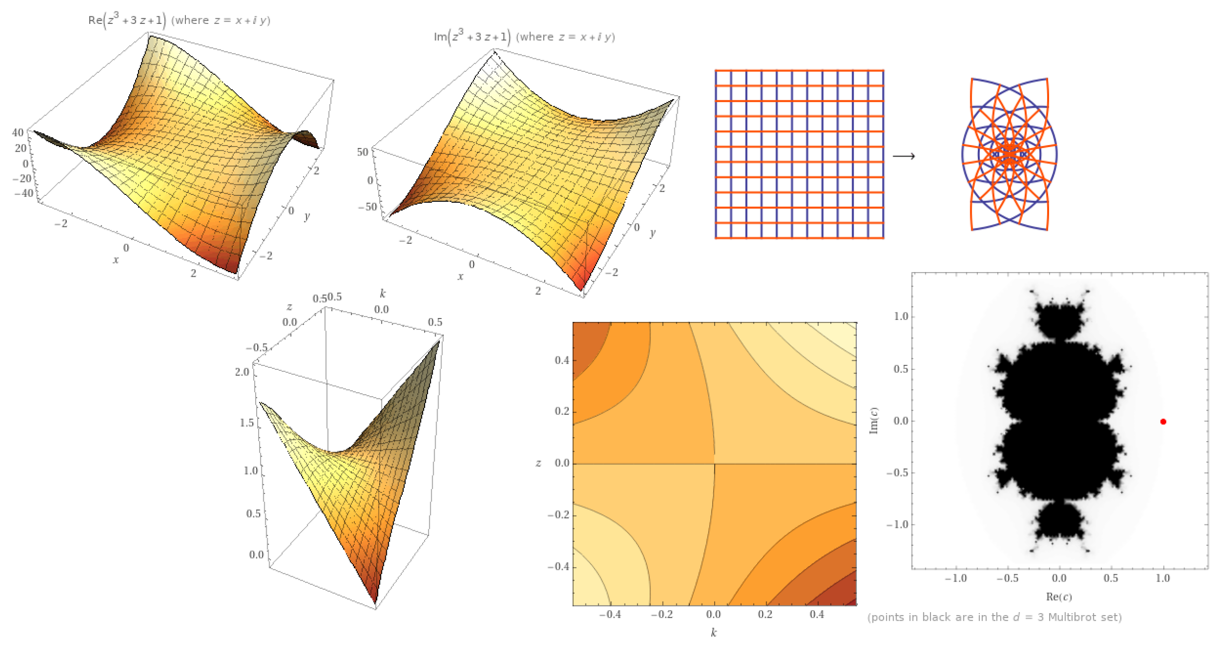
Definition 3.

For the normalized analytic function

$$\phi \left(z\right)=z+\sum _{n=2}^{\infty }{\phi }_n{z}^n,z\in \cup ,$$

the class ${\mathit{M}}_{\tau }\left(\sigma \right)$ is a set of all functions of the form (2)

$$\tau \left(z\right)\left({\displaystyle \frac{z^2{\phi }^{″}\left(z\right)}{\phi \left(z\right)}}\right)+\left({\displaystyle \frac{z{\phi }^{\prime }\left(z\right)}{\phi \left(z\right)}}\right)\prec \sigma \left(z\right),$$

(3)

where $\tau \left(z\right)$ is analytic in $\cup$.

Multibrot Fractal Set Generator

A multibrot set in the complex plane satisfies that the absolute value remains a finite value, taking the formula

$${\mathfrak{P}}_n\left(z\right)=a_n{z}^n+a_{n-1}{z}^{n-1}+\dots +a_0,a_n\ne 0,$$

where $a_i,i=0,\dots ,n$ are constant coefficients. Additionally, a multibrot set Figure 1 is presented by parametric connections such as the full cubic connected locus, which maps the complex number $z\in \cup$ into $\vartheta \left(z\right)=z^3+3\kappa z+1$ (see [15]).

Define a function with the parameter $\kappa$, taking the construction

$$\begin{array}{cc}\hfill {\sigma }_{\kappa }\left(z\right)& =1+\frac{z}{\kappa }\left(\frac{\kappa +z}{\kappa -z}\right)\hfill \\ \hfill & =1+\frac{z}{\kappa }+\frac{\left(2z^2\right)}{{\kappa }^2}+\frac{\left(2z^3\right)}{{\kappa }^3}+\frac{\left(2z^4\right)}{{\kappa }^4}+\frac{\left(2z^5\right)}{{\kappa }^5}+O\left(z^6\right),\left|\kappa \right|>\left|z\right|.\hfill \end{array}$$

(4)

Furthermore, a computation implies that

$$\Re \left({\displaystyle \frac{z{\left(\frac{z}{\kappa }\left(\frac{\kappa +z}{\kappa -z}\right)\right)}^{\prime }}{\frac{z}{\kappa }\left(\frac{\kappa +z}{\kappa -z}\right)}}\right)>0$$

whenever

$$\kappa >0,\kappa -\sqrt{2{\kappa }^2}<\Re \left(z\right)<\kappa .$$

3. Results

In this section, we illustrate our computational results by utilizing the function $\vartheta \left(z\right)$.

Proposition 4.

Let $\phi \in \wedge .$ Define the functions $\mathsf{\Phi }\left(z\right)=\tau \left(z\right)\left({\displaystyle \frac{z^2{\phi }^{″}\left(z\right)}{\phi \left(z\right)}}\right)+\left({\displaystyle \frac{z{\phi }^{\prime }\left(z\right)}{\phi \left(z\right)}}\right)$, ${\sigma }_{\kappa }\left(z\right)=1+\frac{z}{\kappa }\left(\frac{\kappa +z}{\kappa -z}\right)$ and $\vartheta \left(z\right)=1+3\kappa z+z^3.$ If

$$1+\kappa \left(\frac{z{\mathsf{\Phi }}^{\prime }\left(z\right)}{{\left[\mathsf{\Phi }\left(z\right)\right]}^k}\right)\prec {\sigma }_{\kappa }\left(z\right),k=0,1,2,$$

holds then

$$\mathsf{\Phi }\left(z\right)\prec \vartheta \left(z\right)=1+3\kappa z+z^3,z\in \cup$$

where $\kappa \ge max{\kappa }_k,$ and

• ${\kappa }_0=1.07044$;
• ${\kappa }_1=1.27994$;
• ${\kappa }_2=1.5895$.

Proof. 

Step (i): let $k=0\Rightarrow 1+\kappa \left(z{\mathsf{\Phi }}^{\prime }\left(z\right)\right)\prec {\sigma }_{\kappa }\left(z\right)$.

Define a function $X_{\kappa }:\cup \to \mathbb{C}$ with the formula

$$X_{\kappa }\left(z\right)=1+{\displaystyle \frac{2}{\kappa }}\left(log\left(\frac{\kappa }{\kappa -z}\right)-\frac{z}{2\kappa }\right),z\in \cup .$$

Clearly, for the analytic function $X_{\kappa }\left(z\right)$ with $X_{\kappa }\left(0\right)=1,$ we have

$$1+\kappa \left(z{X}_{\kappa }{}^{\prime }\left(z\right)\right)={\sigma }_{\kappa }\left(z\right),z\in \cup .$$

(5)

Define a function

$$\mathfrak{U}\left(z\right):=\frac{z}{\kappa }\left(\frac{\kappa +z}{\kappa -z}\right)$$

which is starlike in ∪ (see [16]). Therefore, for $\mathfrak{G}\left(z\right):=\mathfrak{U}\left(z\right)+1,$ we get

$$\Re \left({\displaystyle \frac{z{\mathfrak{U}}^{\prime }\left(z\right)}{\mathfrak{U}\left(z\right)}}\right)=\Re \left({\displaystyle \frac{z{\mathfrak{G}}^{\prime }\left(z\right)}{\mathfrak{U}\left(z\right)}}\right)>0.$$

Thus, Miller–Mocanu Lemma (see [14], p. 132) admits that

$$1+\kappa \left(z{\mathsf{\Phi }}^{\prime }\left(z\right)\right)\prec 1+\kappa \left(z{X}_{\kappa }^{\prime }\left(z\right)\right)\Rightarrow \mathsf{\Phi }\left(z\right)\prec X_{\kappa }\left(z\right).$$

To finish this conversation, we must show that $X_{\kappa }\left(z\right)\prec {\sigma }_{\kappa }\left(z\right)$ under the necessary condition $\kappa <-1$ or $\kappa >1$ such that

$$1+{\displaystyle \frac{2}{\kappa }}\left(log\left(\frac{\kappa }{\kappa +1}\right)+\frac{1}{2\kappa }\right)=X_{\kappa }(-1)\le X_{\kappa }\left(1\right)=1+{\displaystyle \frac{2}{\kappa }}\left(log\left(\frac{\kappa }{\kappa -1}\right)-\frac{1}{2\kappa }\right).$$

Moreover,

$$1-{\displaystyle \frac{1}{\kappa }}\left(\frac{\kappa -1}{\kappa +1}\right)={\sigma }_{\kappa }(-1)\le {\sigma }_{\kappa }\left(1\right)=1+{\displaystyle \frac{1}{\kappa }}\left(\frac{\kappa +1}{\kappa -1}\right)$$

whenever $-1<\kappa <0$ and $\kappa >1.$ Hence, we obtain

$$1-{\displaystyle \frac{1}{\kappa }}\left(\frac{\kappa -1}{\kappa +1}\right)\le X_{\kappa }(-1)\le X_{\kappa }\left(1\right)\le 1+{\displaystyle \frac{1}{\kappa }}\left(\frac{\kappa +1}{\kappa -1}\right)$$

whenever $\kappa >1.$ Finally, we have that

$$X_{\kappa }\left(z\right)\prec \vartheta \left(z\right)=1+3\kappa z+z^3$$

when

$$-3\kappa \le X_{\kappa }(-1)\le X_{\kappa }\left(1\right)\le 2+3\kappa$$

which is provided

$$\kappa \ge {\kappa }_0=1.07044>1.$$

This implies the relations

$$X_{\kappa }\left(z\right)\prec \vartheta \left(z\right)\Rightarrow \mathsf{\Phi }\left(z\right)\prec \vartheta \left(z\right),z\in \cup .$$

Step (ii): assume that $k=1\Rightarrow 1+\kappa \left(\frac{z{\mathsf{\Phi }}^{\prime }\left(z\right)}{\mathsf{\Phi }\left(z\right)}\right)\prec {\sigma }_{\kappa }\left(z\right)$.

Define a function $Y_{\kappa }:\cup \to \mathbb{C}$ by

$$Y_{\kappa }\left(z\right)=exp\left({\displaystyle \frac{2log({\displaystyle \frac{\kappa }{\kappa -z}})-\frac{z}{\kappa }}{\kappa }}\right).$$

Obviously, the analytic function $Y_{\kappa }\left(z\right)$ achieves $Y_{\kappa }\left(0\right)=1$ and

$$1+\kappa \left(\frac{z{Y}_{\kappa }{}^{\prime }\left(z\right)}{Y_{\kappa }\left(z\right)}\right)={\sigma }_{\kappa }\left(z\right),z\in \cup .$$

(6)

By considering $\mathfrak{U}\left(z\right)={\sigma }_{\kappa }\left(z\right)-1$, which is starlike in ∪ and $\mathfrak{W}\left(z\right)=\mathfrak{U}\left(z\right)+1,$ we attain

$$\Re \left({\displaystyle \frac{z{\mathfrak{U}}^{\prime }\left(z\right)}{\mathfrak{U}\left(z\right)}}\right)=\Re \left({\displaystyle \frac{z{\mathfrak{W}}^{\prime }\left(z\right)}{\mathfrak{U}\left(z\right)}}\right)>0,z\in \cup .$$

Thus, the Miller–Mocanu Lemma yields

$$1+\kappa \left({\displaystyle \frac{z{\mathsf{\Phi }}^{\prime }\left(z\right)}{\mathsf{\Phi }\left(z\right)}}\right)\prec 1+\kappa \left({\displaystyle \frac{z{Y}_{\kappa }^{\prime }\left(z\right)}{Y_{\kappa }\left(z\right)}}\right)\Rightarrow \mathsf{\Phi }\left(z\right)\prec Y_{\kappa }\left(z\right).$$

Proceeding, we have the following inequality

$$exp\left({\displaystyle \frac{2log({\displaystyle \frac{\kappa }{\kappa +1}})+\frac{1}{\kappa }}{\kappa }}\right)=Y_{\kappa }(-1)\le Y_{\kappa }\left(1\right)=exp\left({\displaystyle \frac{2log({\displaystyle \frac{\kappa }{\kappa -1}})-\frac{1}{\kappa }}{\kappa }}\right)$$

when $\kappa >1$ or $\kappa <-1$. In addition, we have $Y_{\kappa }\left(z\right)\prec {\sigma }_{\kappa }\left(z\right)$ provided that for $\kappa >1$, the inequality

$${\sigma }_{\kappa }(-1)\le Y_{\kappa }(-1)\le Y_{\kappa }\left(1\right)\le {\sigma }_{\kappa }(+1)$$

holds. Thus, for $\kappa \ge {\kappa }_1=1.27994$, we get

$$Y_{\kappa }\left(z\right)\prec \vartheta \left(z\right)=1+3\kappa z+z^3$$

when

$$-3\kappa \le Y_{\kappa }(-1)\le Y_{\kappa }\left(1\right)\le 2+3\kappa$$

This yields the following subordination

$$Y_{\kappa }\left(z\right)\prec \vartheta \left(z\right)\Rightarrow \mathsf{\Phi }\left(z\right)\prec \vartheta \left(z\right),z\in \cup .$$

Step (iii): Let $k=2\Rightarrow 1+\kappa \left(\frac{z{\mathsf{\Phi }}^{\prime }\left(z\right)}{{\mathsf{\Phi }}^2\left(z\right)}\right)\prec {\sigma }_{\kappa }\left(z\right),$ then we obtain the following construction.

Define a function $D_{\kappa }:\cup \to \mathbb{C}$ formulated by the design

$$D_{\kappa }\left(z\right)={\left(1-{\displaystyle \frac{2}{\kappa }}\left(log\left(\frac{\kappa }{\kappa -z}\right)-\frac{z}{2\kappa }\right)\right)}^{-1}.$$

Clearly, for the analytic function $D_{\kappa }\left(z\right),$ we have that $D_{\kappa }\left(0\right)=1$ and

$$1+\kappa \left(\frac{z{D}_{\kappa }{}^{\prime }\left(z\right)}{D_{\kappa }^2\left(z\right)}\right)={\sigma }_{\kappa }\left(z\right),z\in \cup .$$

(7)

By considering the functions $\mathfrak{U}\left(z\right)={\sigma }_{\kappa }\left(z\right)-1$, which is starlike in ∪ and $\mathfrak{W}\left(z\right)=\mathfrak{U}\left(z\right)+1,$ we receive

$$\Re \left({\displaystyle \frac{z{\mathfrak{U}}^{\prime }\left(z\right)}{\mathfrak{U}\left(z\right)}}\right)=\Re \left({\displaystyle \frac{z{\mathfrak{W}}^{\prime }\left(z\right)}{\mathfrak{U}\left(z\right)}}\right)>0,z\in \cup .$$

Hence, the Miller-Mocanu Lemma yields

$$1+\kappa \left({\displaystyle \frac{z{\mathsf{\Phi }}^{\prime }\left(z\right)}{{\mathsf{\Phi }}^2\left(z\right)}}\right)\prec 1+\kappa \left({\displaystyle \frac{z{D}_{\kappa }^{\prime }\left(z\right)}{D_{\kappa }^2\left(z\right)}}\right)\Rightarrow \mathsf{\Phi }\left(z\right)\prec D_{\kappa }\left(z\right).$$

Accordingly, for $\kappa <-1$ or $\kappa >1.50957$, we obtain

$${\left(1-{\displaystyle \frac{2}{\kappa }}\left(log\left(\frac{\kappa }{\kappa +1}\right)+\frac{1}{2\kappa }\right)\right)}^{-1}\le D_{\kappa }(-1)\le D_{\kappa }\left(1\right)={\left(1-{\displaystyle \frac{2}{\kappa }}\left(log\left(\frac{\kappa }{\kappa -1}\right)-\frac{1}{2\kappa }\right)\right)}^{-1}.$$

Moreover, the subordination $D_{\kappa }\left(z\right)\prec {\sigma }_{\kappa }\left(z\right)$ when $\kappa =1.7723>1.50957$ such that

$${\sigma }_{\kappa }(-1)\le D_{\kappa }(-1)\le D_{\kappa }\left(1\right)\le {\sigma }_{\kappa }\left(1\right).$$

Thus, for $\kappa =1.5895>1.50957$, we have

$$-3\kappa \le D_{\kappa }(-1)\le D_{\kappa }\left(1\right)\le 2+3\kappa .$$

Consequently, this implies that

$$D_{\kappa }\left(z\right)\prec \vartheta \left(z\right)\Rightarrow \mathsf{\Phi }\left(z\right)\prec \vartheta \left(z\right),z\in \cup .$$

□

Proposition 4 can be generalized by assuming an analytic function $\rho \left(z\right),z\in \cup$ such that $\rho \left(0\right)=1$. The proof is similar to the proof of Proposition 4; therefore, we omit it.

Proposition 5.

Let $\rho \in \mathbb{H}$ (the set of analytic functions in the open unit disk) such that $\rho \left(0\right)=1,{\rho }^{\prime }\left(0\right)>1,\Re \left(\rho \left(z\right)\right)>0$ and let

$${\sigma }_{\kappa }\left(z\right)=1+\frac{z}{\kappa }\left(\frac{\kappa +z}{\kappa -z}\right),z\in \cup ,$$

where κ is a real parameter. If one of the differential inequalities hold

$$1+\kappa \left(\frac{z{\rho }^{\prime }\left(z\right)}{{\left[\rho \left(z\right)\right]}^k}\right)\prec {\sigma }_{\kappa }\left(z\right),k=0,1,2,$$

then

$$\rho \left(z\right)\prec \vartheta \left(z\right)=1+3\kappa z+z^3,z\in \cup ,\kappa >1.5895.$$

In the next result, we consider two different parameters $\kappa$ and $\beta$.

Proposition 6.

Consider $\phi \in \wedge$ such that

$$1+\kappa \left(\frac{z{\mathsf{\Phi }}^{\prime }\left(z\right)}{{\left[\mathsf{\Phi }\left(z\right)\right]}^k}\right)\prec {\sigma }_{\kappa }\left(z\right),k=0,1,2,$$

where $\mathsf{\Phi }\left(z\right)=\tau \left(z\right)\left({\displaystyle \frac{z^2{\phi }^{″}\left(z\right)}{\phi \left(z\right)}}\right)+\left({\displaystyle \frac{z{\phi }^{\prime }\left(z\right)}{\phi \left(z\right)}}\right)$ and ${\sigma }_{\kappa }\left(z\right)=1+\frac{z}{\kappa }\left(\frac{\kappa +z}{\kappa -z}\right),z\in \cup$. Then

$$\mathsf{\Phi }\left(z\right)\prec \vartheta \left(z\right)=1+3\beta z+z^3,z\in \cup$$

when $\beta \ge max{\beta }_k,k=0,1,2$ such that

• ${\beta }_0=max\{{\displaystyle \frac{-\kappa -{\displaystyle \frac{1}{\kappa }}-2log({\displaystyle \frac{\kappa }{\kappa +1}})}{3\kappa }},{\displaystyle \frac{-\kappa -{\displaystyle \frac{1}{\kappa }}+2log({\displaystyle \frac{\kappa }{\kappa -1}})}{3\kappa }}\},\kappa >1$;
• $\beta {}_1=max\left\{-{\displaystyle \frac{1}{3}}{e}^{(1/{\kappa }^2)}{\left({\displaystyle \frac{\kappa }{\kappa +1}}\right)}^{(2/\kappa )},{\displaystyle \frac{1}{3}}\left(e^{(-1/{\kappa }^2)}{\left({\displaystyle \frac{\kappa }{\kappa -1}}\right)}^{(2/\kappa )}-2\right)\right\},\kappa >1$;
• ${\beta }_2=max\{{\displaystyle \frac{-{\kappa }^2}{3({\kappa }^2-2\kappa log({\displaystyle \frac{\kappa }{\kappa +1}})-1)}},{\displaystyle \frac{1}{3}}\left({\displaystyle \frac{{\kappa }^2}{{\kappa }^2-2\kappa log({\displaystyle \frac{\kappa }{\kappa -1}})+1}}-2\right)\},\kappa >1$.

Proof. 

Step (i): suppose that $k=0\Rightarrow 1+\kappa \left(z{\mathsf{\Phi }}^{\prime }\left(z\right)\right)\prec {\sigma }_{\kappa }\left(z\right)$.

Define an analytic function $X_{\kappa }:\cup \to \mathbb{C}$ constructed as follows:

$$X_{\kappa }\left(z\right)=1+{\displaystyle \frac{2}{\kappa }}\left(log\left(\frac{\kappa }{\kappa -z}\right)-\frac{z}{2\kappa }\right),z\in \cup .$$

Thus, we obtain $X_{\kappa }\left(0\right)=1$ and

$$1+\kappa \left(z{X}_{\kappa }{}^{\prime }\left(z\right)\right)={\sigma }_{\kappa }\left(z\right),z\in \cup .$$

(8)

Define a function

$$\mathfrak{U}\left(z\right):=\frac{z}{\kappa }\left(\frac{\kappa +z}{\kappa -z}\right),$$

which is starlike in ∪ (see [16]). Therefore, for $\mathfrak{G}\left(z\right):=\mathfrak{U}\left(z\right)+1,$ we get

$$\Re \left({\displaystyle \frac{z{\mathfrak{U}}^{\prime }\left(z\right)}{\mathfrak{U}\left(z\right)}}\right)=\Re \left({\displaystyle \frac{z{\mathfrak{G}}^{\prime }\left(z\right)}{\mathfrak{U}\left(z\right)}}\right)>0.$$

Thus, Miller–Mocanu Lemma (see [14], p. 132) admits that

$$1+\kappa \left(z{\mathsf{\Phi }}^{\prime }\left(z\right)\right)\prec 1+\kappa \left(z{X}_{\kappa }^{\prime }\left(z\right)\right)\Rightarrow \mathsf{\Phi }\left(z\right)\prec X_{\kappa }\left(z\right).$$

To finish this conversation, we must show that $X_{\kappa }\left(z\right)\prec {\sigma }_{\kappa }\left(z\right)$ under the necessary condition $\kappa <-1$ or $\kappa >1$ such that

$$1+{\displaystyle \frac{2}{\kappa }}\left(log\left(\frac{\kappa }{\kappa +1}\right)+\frac{1}{2\kappa }\right)=X_{\kappa }(-1)\le X_{\kappa }\left(1\right)=1+{\displaystyle \frac{2}{\kappa }}\left(log\left(\frac{\kappa }{\kappa -1}\right)-\frac{1}{2\kappa }\right).$$

Moreover,

$$1-{\displaystyle \frac{1}{\kappa }}\left(\frac{\kappa -1}{\kappa +1}\right)={\sigma }_{\kappa }(-1)\le {\sigma }_{\kappa }\left(1\right)=1+{\displaystyle \frac{1}{\kappa }}\left(\frac{\kappa +1}{\kappa -1}\right)$$

whenever $-1<\kappa <0$ and $\kappa >1$. Hence, we obtain

$$1-{\displaystyle \frac{1}{\kappa }}\left(\frac{\kappa -1}{\kappa +1}\right)\le X_{\kappa }(-1)\le X_{\kappa }\left(1\right)\le 1+{\displaystyle \frac{1}{\kappa }}\left(\frac{\kappa +1}{\kappa -1}\right)$$

whenever $\kappa >1$. Finally, we have that

$$X_{\kappa }\left(z\right)\prec \vartheta \left(z\right)=1+3\beta z+z^3$$

when

$$-3\beta \le X_{\kappa }(-1)\le X_{\kappa }\left(1\right)\le 2+3\beta$$

which is provided

$$\begin{array}{cc}\hfill \beta & =max\{{\displaystyle \frac{-\kappa -{\displaystyle \frac{1}{\kappa }}-2log({\displaystyle \frac{\kappa }{\kappa +1}})}{3\kappa }},{\displaystyle \frac{-\kappa -{\displaystyle \frac{1}{\kappa }}+2log({\displaystyle \frac{\kappa }{\kappa -1}})}{3\kappa }}\}\hfill \\ \hfill & =max\{{\displaystyle \frac{1}{3}}(2log\left(2\right)-2),{\displaystyle \frac{1}{12}}(4log\left(2\right)-5)\}\hfill \\ \hfill & \approx max\{-0.204569,-0.185618\}\hfill \\ \hfill & =-0.185618,\kappa >1.\hfill \end{array}$$

Hence, we have

$$X_{\kappa }\left(z\right)\prec \vartheta \left(z\right)\Rightarrow \mathsf{\Phi }\left(z\right)\prec \vartheta \left(z\right),z\in \cup .$$

Step (ii): put $k=1\Rightarrow 1+\kappa \left(\frac{z{\mathsf{\Phi }}^{\prime }\left(z\right)}{\mathsf{\Phi }\left(z\right)}\right)\prec {\sigma }_{\kappa }\left(z\right)$.

Define an analytic function $Y_{\kappa }:\cup \to \mathbb{C}$ formulating by the structure

$$Y_{\kappa }\left(z\right)=exp\left({\displaystyle \frac{2log({\displaystyle \frac{\kappa }{\kappa -z}})-\frac{z}{\kappa }}{\kappa }}\right).$$

Obviously, $Y_{\kappa }\left(z\right)$ is satisfying $Y_{\kappa }\left(0\right)=1$ and

$$1+\kappa \left(\frac{z{Y}_{\kappa }{}^{\prime }\left(z\right)}{Y_{\kappa }\left(z\right)}\right)={\sigma }_{\kappa }\left(z\right),z\in \cup .$$

(9)

By considering $\mathfrak{U}\left(z\right)={\sigma }_{\kappa }\left(z\right)-1$, which is starlike in ∪ and $\mathfrak{W}\left(z\right)=\mathfrak{U}\left(z\right)+1,$ we attain

$$\Re \left({\displaystyle \frac{z{\mathfrak{U}}^{\prime }\left(z\right)}{\mathfrak{U}\left(z\right)}}\right)=\Re \left({\displaystyle \frac{z{\mathfrak{W}}^{\prime }\left(z\right)}{\mathfrak{U}\left(z\right)}}\right)>0,z\in \cup .$$

Thus, Miller-Mocanu Lemma implies

$$1+\kappa \left({\displaystyle \frac{z{\mathsf{\Phi }}^{\prime }\left(z\right)}{\mathsf{\Phi }\left(z\right)}}\right)\prec 1+\kappa \left({\displaystyle \frac{z{Y}_{\kappa }^{\prime }\left(z\right)}{Y_{\kappa }\left(z\right)}}\right)\Rightarrow \mathsf{\Phi }\left(z\right)\prec Y_{\kappa }\left(z\right).$$

Proceeding, the following inequality indicates

$$exp\left({\displaystyle \frac{2log({\displaystyle \frac{\kappa }{\kappa +1}})+{\displaystyle \frac{1}{\kappa }}}{\kappa }}\right)=Y_{\kappa }(-1)\le Y_{\kappa }\left(1\right)=exp\left({\displaystyle \frac{2log({\displaystyle \frac{\kappa }{\kappa -1}})-{\displaystyle \frac{1}{\kappa }}}{\kappa }}\right)$$

if $\kappa >1$ or $\kappa <-1$. In addition, we have $Y_{\kappa }\left(z\right)\prec {\sigma }_{\kappa }\left(z\right)$ provided that for $\kappa >1$ the inequality

$${\sigma }_{\kappa }(-1)\le Y_{\mu }(-1)\le Y_{\mu }\left(1\right)\le {\sigma }_{\kappa }(+1)$$

holds. Thus, we have

$$Y_{\kappa }\left(z\right)\prec \vartheta \left(z\right)=1+3\beta z+z^3$$

when

$$-3\beta \le Y_{\kappa }(-1)\le Y_{\kappa }\left(1\right)\le 2+3\beta$$

satisfying

$$\begin{array}{cc}\hfill \beta & =max\{-{\displaystyle \frac{1}{3}}{e}^{(1/{\kappa }^2)}{\left({\displaystyle \frac{\kappa }{\kappa +1}}\right)}^{(2/\kappa )},{\displaystyle \frac{1}{3}}\left(e^{(-1/{\kappa }^2)}{\left({\displaystyle \frac{\kappa }{\kappa -1}}\right)}^{(2/\kappa )}-2\right)\}\hfill \\ & =max\{(-0.333333){\left(2.71828\right)}^{(1/{\kappa }^2)}{\left({\displaystyle \frac{\kappa }{\kappa +1}}\right)}^{(2/\kappa )},\left(0.333333\right)\left({2.71828}^{(-1/{\kappa }^2)}{\left({\displaystyle \frac{\kappa }{\kappa -1}}\right)}^{(2/\kappa )}-2\right)\}\hfill \\ & \approx -0.333333,\kappa >1.\hfill \end{array}$$

(10)

This leads to the following subordination

$$Y_{\kappa }\left(z\right)\prec \vartheta \left(z\right)\Rightarrow \mathsf{\Phi }\left(z\right)\prec \vartheta \left(z\right),z\in \cup .$$

Step (iii): consume that $k=2\Rightarrow 1+\kappa \left(\frac{z{\mathsf{\Phi }}^{\prime }\left(z\right)}{{\mathsf{\Phi }}^2\left(z\right)}\right)\prec {\sigma }_{\kappa }\left(z\right)$.

Define a function $D_{\kappa }:\cup \to \mathbb{C}$ formulating by the design

$$D_{\kappa }\left(z\right)={\left(1-{\displaystyle \frac{2}{\kappa }}\left(log\left(\frac{\kappa }{\kappa -z}\right)-\frac{z}{2\kappa }\right)\right)}^{-1}.$$

Clearly, $D_{\kappa }\left(0\right)=1$ and

$$1+\kappa \left(\frac{z{D}_{\kappa }{}^{\prime }\left(z\right)}{D_{\kappa }^2\left(z\right)}\right)={\sigma }_{\kappa }\left(z\right),z\in \cup .$$

(11)

By considering the functions $\mathfrak{U}\left(z\right)={\sigma }_{\kappa }\left(z\right)-1$, which is starlike in ∪ and $\mathfrak{W}\left(z\right)=\mathfrak{U}\left(z\right)+1,$ we receive

$$\Re \left({\displaystyle \frac{z{\mathfrak{U}}^{\prime }\left(z\right)}{\mathfrak{U}\left(z\right)}}\right)=\Re \left({\displaystyle \frac{z{\mathfrak{W}}^{\prime }\left(z\right)}{\mathfrak{U}\left(z\right)}}\right)>0,z\in \cup .$$

Hence, the Miller-Mocanu Lemma implies

$$1+\kappa \left({\displaystyle \frac{z{\mathsf{\Phi }}^{\prime }\left(z\right)}{{\mathsf{\Phi }}^2\left(z\right)}}\right)\prec 1+\kappa \left({\displaystyle \frac{z{D}_{\kappa }^{\prime }\left(z\right)}{D_{\kappa }^2\left(z\right)}}\right)\Rightarrow \mathsf{\Phi }\left(z\right)\prec D_{\kappa }\left(z\right).$$

Accordingly, for $\kappa <-1$ or $\kappa >1.50957$, we obtain

$${\left(1-{\displaystyle \frac{2}{\kappa }}\left(log\left(\frac{\kappa }{\kappa +1}\right)+\frac{1}{2\kappa }\right)\right)}^{-1}\le D_{\kappa }(-1)\le D_{\kappa }\left(1\right)={\left(1-{\displaystyle \frac{2}{\kappa }}\left(log\left(\frac{\kappa }{\kappa -1}\right)-\frac{1}{2\kappa }\right)\right)}^{-1}.$$

Moreover, the subordination $D_{\kappa }\left(z\right)\prec {\sigma }_{\kappa }\left(z\right)$ when $\kappa =1.7723>1.50957$ such that

$${\sigma }_{\kappa }(-1)\le D_{\kappa }(-1)\le D_{\kappa }\left(1\right)\le {\sigma }_{\kappa }\left(1\right).$$

Thus, if

$$\begin{array}{cc}\hfill \beta & =max\{{\displaystyle \frac{-{\kappa }^2}{3({\kappa }^2-2\kappa log({\displaystyle \frac{\kappa }{\kappa +1}})-1)}},{\displaystyle \frac{1}{3}}\left({\displaystyle \frac{{\kappa }^2}{{\kappa }^2-2\kappa log({\displaystyle \frac{\kappa }{\kappa -1}})+1}}-2\right)\}\hfill \\ \hfill & =max\left\{{\displaystyle \frac{1}{3}},-{\displaystyle \frac{1}{3}}\right\}\hfill \\ \hfill & \approx 0.333333,\kappa >1,\hfill \end{array}$$

then we have

$$-3\beta \le D_{\kappa }(-1)\le D_{\kappa }\left(1\right)\le 2+3\beta .$$

Consequently, this implies that

$$D_{\kappa }\left(z\right)\prec \vartheta \left(z\right)\Rightarrow \mathsf{\Phi }\left(z\right)\prec \vartheta \left(z\right),z\in \cup .$$

□

Proposition 6 can be extended by consuming an analytic function $\varrho \left(z\right),z\in \cup$ such that $\varrho \left(0\right)=1.$ The proof is similar to the proof of Proposition 4; therefore, we omit it.

Proposition 7.

Let $\varrho \in \mathbb{H}$ such that $\varrho \left(0\right)=1,{\varrho }^{\prime }\left(0\right)>1,\Re \left(\varrho \left(z\right)\right)>0$ and let

$${\sigma }_{\kappa }\left(z\right)=1+\frac{z}{\kappa }\left(\frac{\kappa +z}{\kappa -z}\right),z\in \cup ,$$

where κ is a real parameter. If one of the differential inequalities holds

$$1+\kappa \left(\frac{z{\varrho }^{\prime }\left(z\right)}{{\left[\varrho \left(z\right)\right]}^k}\right)\prec {\sigma }_{\kappa }\left(z\right),k=0,1,2,$$

then

$$\varrho \left(z\right)\prec \vartheta \left(z\right)=1+3\beta z+z^3,z\in \cup ,\beta >1/3.$$

We proceed to consider three parameters $\alpha ,\beta$ and $\kappa$. We obtain the following result:

Proposition 8.

Let the function $\phi \in \wedge$ designing the inequality

$$1+\alpha \left(\frac{z{\mathsf{\Phi }}^{\prime }\left(z\right)}{{\left[\mathsf{\Phi }\left(z\right)\right]}^k}\right)\prec {\sigma }_{\kappa }\left(z\right),k=0,1,2,$$

where $\mathsf{\Phi }\left(z\right)=\tau \left(z\right)\left({\displaystyle \frac{z^2{\phi }^{″}\left(z\right)}{\phi \left(z\right)}}\right)+\left({\displaystyle \frac{z{\phi }^{\prime }\left(z\right)}{\phi \left(z\right)}}\right)$ and ${\sigma }_{\kappa }\left(z\right)=1+\frac{z}{\kappa }\left(\frac{\kappa +z}{\kappa -z}\right),z\in \cup$. Then

$$\mathsf{\Phi }\left(z\right)\prec \vartheta \left(z\right)=1+3\beta z+z^3,z\in \cup$$

when $\beta \ge max{\beta }_k,k=0,1,2$ such that

• ${\beta }_0=max\{{\displaystyle \frac{-({\alpha }^2+2\alpha log({\displaystyle \frac{\alpha }{\alpha +1}})+1)}{3{\alpha }^2}},{\displaystyle \frac{-({\alpha }^2-2\alpha log({\displaystyle \frac{\alpha }{\alpha -1}})+1)}{3{\alpha }^2}}\}\approx {\displaystyle \frac{-1}{3}}$

  $$\left(\alpha \ge -0.211728,\kappa =max\{{\displaystyle \frac{0.5(2\alpha -2.82843|\alpha \left|\right)}{\left(2.82843\right|\alpha |-3\alpha )}},{\displaystyle \frac{0.5\left(2.82843\alpha \right|\alpha |-2{\alpha }^2)}{\left(\alpha \right(2.82843\left|\alpha \right|-3\alpha \left)\right)}}\}\right);$$
• $\beta {}_1=max\{{\displaystyle \frac{-1}{3}}{\left({\displaystyle \frac{\alpha }{\alpha +1}}\right)}^{(2/\alpha )}{e}^{(1/{\alpha }^2)},{\displaystyle \frac{1}{3}}\left({({\displaystyle \frac{\alpha }{\alpha -1}})}^{(2/\alpha )}{e}^{(-1/{\alpha }^2)}-2\right)\}\approx {\displaystyle \frac{-1}{3}}$

  $$\left(\alpha >1,\kappa \ge -2\right);$$
• ${\beta }_2=max\{{\displaystyle \frac{{\alpha }^2}{-3{\alpha }^2+6\alpha log({\displaystyle \frac{\alpha }{\alpha +1}})+3}},{\displaystyle \frac{1}{3}}\left({\displaystyle \frac{{\alpha }^2}{{\alpha }^2-2\alpha log({\displaystyle \frac{\alpha }{\alpha -1}})+1}}-2\right)\}\approx {\displaystyle \frac{-1}{3}}$

  $$\alpha >1,\kappa ={\displaystyle \frac{{\alpha }^2}{1.41421{\alpha }^2+{\alpha }^2}}=0.4142,$$

Proof. 

Step (i): let $k=0\Rightarrow 1+\alpha \left(z{\mathsf{\Phi }}^{\prime }\left(z\right)\right)\prec {\sigma }_{\kappa }\left(z\right)$.

Define an analytic function $X_{\alpha }:\cup \to \mathbb{C}$ by

$$X_{\alpha }\left(z\right)=1+{\displaystyle \frac{2}{\alpha }}\left(log\left(\frac{\alpha }{\alpha -z}\right)-\frac{z}{2\alpha }\right),z\in \cup .$$

Clearly, $X_{\alpha }\left(0\right)=1$ and

$$1+\alpha \left(z{X}_{\alpha }{}^{\prime }\left(z\right)\right)={\sigma }_{\kappa }\left(z\right),z\in \cup .$$

(12)

Define a function

$$\mathfrak{U}\left(z\right)=\frac{z}{\kappa }\left(\frac{\kappa +z}{\kappa -z}\right)$$

which is starlike in ∪ (see [16]). Therefore, for $\mathfrak{G}\left(z\right):=\mathfrak{U}\left(z\right)+1,$ we get

$$\Re \left({\displaystyle \frac{z{\mathfrak{U}}^{\prime }\left(z\right)}{\mathfrak{U}\left(z\right)}}\right)=\Re \left({\displaystyle \frac{z{\mathfrak{G}}^{\prime }\left(z\right)}{\mathfrak{U}\left(z\right)}}\right)>0.$$

Thus, Miller–Mocanu Lemma implies

$$1+\alpha \left(z{\mathsf{\Phi }}^{\prime }\left(z\right)\right)\prec 1+\alpha \left(z{X}_{\kappa }^{\prime }\left(z\right)\right)\Rightarrow \mathsf{\Phi }\left(z\right)\prec X_{\alpha }\left(z\right).$$

It is clear that $X_{\alpha }\left(z\right)\prec {\sigma }_{\kappa }\left(z\right)$ under the necessary condition $\alpha <-1$ or $\alpha >1$ such that

$$1+{\displaystyle \frac{2}{\alpha }}\left(log\left(\frac{\alpha }{\alpha +1}\right)+\frac{1}{2\alpha }\right)=X_{\alpha }(-1)\le X_{\alpha }\left(1\right)=1+{\displaystyle \frac{2}{\alpha }}\left(log\left(\frac{\alpha }{\alpha -1}\right)-\frac{1}{2\alpha }\right)$$

and

$$1-{\displaystyle \frac{1}{\kappa }}\left(\frac{\kappa -1}{\kappa +1}\right)={\sigma }_{\kappa }(-1)\le {\sigma }_{\kappa }\left(1\right)=1+{\displaystyle \frac{1}{\kappa }}\left(\frac{\kappa +1}{\kappa -1}\right)$$

whenever $-1<\kappa <0$ and $\kappa >1$. Hence, we obtain

$$1-{\displaystyle \frac{1}{\kappa }}\left(\frac{\kappa -1}{\kappa +1}\right)\le X_{\alpha }(-1)\le X_{\alpha }\left(1\right)\le 1+{\displaystyle \frac{1}{\kappa }}\left(\frac{\kappa +1}{\kappa -1}\right)$$

whenever

$$\alpha \ge -0.211728,\kappa =max\{{\displaystyle \frac{0.5(2\alpha -2.82843|\alpha \left|\right)}{\left(2.82843\right|\alpha |-3\alpha )}},{\displaystyle \frac{0.5\left(2.82843\alpha \right|\alpha |-2{\alpha }^2)}{\left(\alpha \right(2.82843\left|\alpha \right|-3\alpha \left)\right)}}\}.$$

Finally, we have that

$$X_{\alpha }\left(z\right)\prec \vartheta \left(z\right)=1+3\beta z+z^3$$

when

$$-3\beta \le X_{\alpha }(-1)\le X_{\alpha }\left(1\right)\le 2+3\beta$$

which is provided

$$\begin{array}{cc}\hfill \beta & =max\{{\displaystyle \frac{-({\alpha }^2+2\alpha log({\displaystyle \frac{\alpha }{\alpha +1}})+1)}{3{\alpha }^2}},{\displaystyle \frac{-({\alpha }^2-2\alpha log({\displaystyle \frac{\alpha }{\alpha -1}})+1)}{3{\alpha }^2}}\}\hfill \\ \hfill & \approx {\displaystyle \frac{-1}{3}}\hfill \\ \hfill & \left(\alpha >0,\kappa =max\{{\displaystyle \frac{0.5(2\alpha -2.82843|\alpha \left|\right)}{\left(2.82843\right|\alpha |-3\alpha )}},{\displaystyle \frac{0.5\left(2.82843\alpha \right|\alpha |-2{\alpha }^2)}{\left(\alpha \right(2.82843\left|\alpha \right|-3\alpha \left)\right)}}\}\right).\hfill \end{array}$$

Which implies that

$$X_{\alpha }\left(z\right)\prec \vartheta \left(z\right)\Rightarrow \mathsf{\Phi }\left(z\right)\prec \vartheta \left(z\right),z\in \cup .$$

Step (ii): consider $k=1\Rightarrow 1+\alpha \left(\frac{z{\mathsf{\Phi }}^{\prime }\left(z\right)}{\mathsf{\Phi }\left(z\right)}\right)\prec {\sigma }_{\kappa }\left(z\right)$.

Define an analytic function $Y_{\alpha }:\cup \to \mathbb{C}$ by

$$Y_{\alpha }\left(z\right)=exp\left({\displaystyle \frac{2log({\displaystyle \frac{\alpha }{\alpha -z}})-\frac{z}{\alpha }}{\alpha }}\right).$$

Obviously, $Y_{\alpha }\left(0\right)=1$ and

$$1+\alpha \left(\frac{z{Y}_{\alpha }{}^{\prime }\left(z\right)}{Y_{\alpha }\left(z\right)}\right)={\sigma }_{\kappa }\left(z\right),z\in \cup .$$

(13)

By considering $\mathfrak{U}\left(z\right)={\sigma }_{\kappa }\left(z\right)-1$, which is starlike in ∪ and $\mathfrak{W}\left(z\right)=\mathfrak{U}\left(z\right)+1$, we attain

$$\Re \left({\displaystyle \frac{z{\mathfrak{U}}^{\prime }\left(z\right)}{\mathfrak{U}\left(z\right)}}\right)=\Re \left({\displaystyle \frac{z{\mathfrak{W}}^{\prime }\left(z\right)}{\mathfrak{U}\left(z\right)}}\right)>0,z\in \cup .$$

Thus, Miller–Mocanu Lemma implies

$$1+\alpha \left({\displaystyle \frac{z{\mathsf{\Phi }}^{\prime }\left(z\right)}{\mathsf{\Phi }\left(z\right)}}\right)\prec 1+\alpha \left({\displaystyle \frac{z{Y}_{\alpha }^{\prime }\left(z\right)}{Y_{\alpha }\left(z\right)}}\right)\Rightarrow \mathsf{\Phi }\left(z\right)\prec Y_{\alpha }\left(z\right).$$

Proceeding, the following inequality holds when $\alpha \ne 0$,

$$exp\left({\displaystyle \frac{2log({\displaystyle \frac{\alpha }{\alpha +1}})+{\displaystyle \frac{1}{\alpha }}}{\alpha }}\right)=Y_{\alpha }(-1)\le Y_{\alpha }\left(1\right)=exp\left({\displaystyle \frac{2log({\displaystyle \frac{\alpha }{\alpha -1}})-{\displaystyle \frac{1}{\alpha }}}{\alpha }}\right)$$

In addition, we have $Y_{\alpha }\left(z\right)\prec {\sigma }_{\kappa }\left(z\right)$ whenever

$$1-{\displaystyle \frac{1}{\kappa }}\left(\frac{\kappa -1}{\kappa +1}\right)\le Y_{\alpha }(-1)\le Y_{\alpha }\left(1\right)\le 1+{\displaystyle \frac{1}{\kappa }}\left(\frac{\kappa +1}{\kappa -1}\right)$$

$$\left(\alpha >1,\kappa \ge -2\right)$$

holds. Thus, we have

$$Y_{\alpha }\left(z\right)\prec \vartheta \left(z\right)=1+3\beta z+z^3$$

when

$$-3\beta \le Y_{\alpha }(-1)\le Y_{\alpha }\left(1\right)\le 2+3\beta$$

satisfying

$$\begin{array}{cc}\hfill \beta & =max\{{\displaystyle \frac{-1}{3}}{\left({\displaystyle \frac{\alpha }{\alpha +1}}\right)}^{(2/\alpha )}{e}^{(1/{\alpha }^2)},{\displaystyle \frac{1}{3}}\left({({\displaystyle \frac{\alpha }{\alpha -1}})}^{(2/\alpha )}{e}^{(-1/{\alpha }^2)}-2\right)\}\hfill \\ \hfill & \approx -0.333333,\alpha >1.\hfill \end{array}$$

Consequently, we have the following subordination

$$Y_{\alpha }\left(z\right)\prec \vartheta \left(z\right)\Rightarrow \mathsf{\Phi }\left(z\right)\prec \vartheta \left(z\right),z\in \cup .$$

Step(iii): put $k=2\Rightarrow 1+\alpha \left(\frac{z{\mathsf{\Phi }}^{\prime }\left(z\right)}{{\mathsf{\Phi }}^2\left(z\right)}\right)\prec {\sigma }_{\kappa }\left(z\right)$.

Define an analytic function $D_{\alpha }:\cup \to \mathbb{C}$ by

$$D_{\alpha }\left(z\right)={\left(1-{\displaystyle \frac{2}{\alpha }}\left(log\left(\frac{\alpha }{\alpha -z}\right)-\frac{z}{2\alpha }\right)\right)}^{-1}.$$

Clearly, $D_{\alpha }\left(0\right)=1$ and

$$1+\alpha \left(\frac{z{D}_{\alpha }{}^{\prime }\left(z\right)}{D_{\alpha }^2\left(z\right)}\right)={\sigma }_{\kappa }\left(z\right),z\in \cup .$$

(14)

By considering the functions $\mathfrak{U}\left(z\right)={\sigma }_{\kappa }\left(z\right)-1$, which is starlike in ∪ and $\mathfrak{W}\left(z\right)=\mathfrak{U}\left(z\right)+1,$ we receive

$$\Re \left({\displaystyle \frac{z{\mathfrak{U}}^{\prime }\left(z\right)}{\mathfrak{U}\left(z\right)}}\right)=\Re \left({\displaystyle \frac{z{\mathfrak{W}}^{\prime }\left(z\right)}{\mathfrak{U}\left(z\right)}}\right)>0,z\in \cup .$$

Hence, the Miller–Mocanu Lemma yields

$$1+\alpha \left({\displaystyle \frac{z{\mathsf{\Phi }}^{\prime }\left(z\right)}{{\mathsf{\Phi }}^2\left(z\right)}}\right)\prec 1+\alpha \left({\displaystyle \frac{z{D}_{\alpha }^{\prime }\left(z\right)}{D_{\alpha }^2\left(z\right)}}\right)\Rightarrow \mathsf{\Phi }\left(z\right)\prec D_{\alpha }\left(z\right).$$

Accordingly, for $\alpha <-1$ or $\alpha >1.50957$, we obtain

$${\left(1-{\displaystyle \frac{2}{\alpha }}\left(log\left(\frac{\alpha }{\alpha +1}\right)+\frac{1}{2\alpha }\right)\right)}^{-1}\le D_{\alpha }(-1)\le D_{\alpha }\left(1\right)={\left(1-{\displaystyle \frac{2}{\alpha }}\left(log\left(\frac{\alpha }{\kappa -1}\right)-\frac{1}{2\alpha }\right)\right)}^{-1}.$$

Moreover, the subordination $D_{\alpha }\left(z\right)\prec {\sigma }_{\kappa }\left(z\right)$ when

$$\alpha >1,\kappa ={\displaystyle \frac{{\alpha }^2}{1.41421{\alpha }^2+{\alpha }^2}}=0.4142,$$

such that

$$1-{\displaystyle \frac{1}{\kappa }}\left(\frac{\kappa -1}{\kappa +1}\right)\le D_{\alpha }(-1)\le D_{\alpha }\left(1\right)\le 1+{\displaystyle \frac{1}{\kappa }}\left(\frac{\kappa +1}{\kappa -1}\right).$$

Thus, if

$$\begin{array}{cc}\hfill \beta & =max\{{\displaystyle \frac{{\alpha }^2}{-3{\alpha }^2+6\alpha log({\displaystyle \frac{\alpha }{\alpha +1}})+3}},{\displaystyle \frac{1}{3}}\left({\displaystyle \frac{{\alpha }^2}{{\alpha }^2-2\alpha log({\displaystyle \frac{\alpha }{\alpha -1}})+1}}-2\right)\}\hfill \\ \hfill & =max\{{\displaystyle \frac{-1}{3}},{\displaystyle \frac{-1}{3}}\}\hfill \\ \hfill & \approx -0.333333,\hfill \end{array}$$

$$\left(\alpha >1,\kappa ={\displaystyle \frac{{\alpha }^2}{1.41421{\alpha }^2+{\alpha }^2}}\right),$$

then we have

$$-3\beta \le D_{\alpha }(-1)\le D_{\alpha }\left(1\right)\le 2+3\beta .$$

Consequently, this implies that

$$D_{\alpha }\left(z\right)\prec \vartheta \left(z\right)\Rightarrow \mathsf{\Phi }\left(z\right)\prec \vartheta \left(z\right),z\in \cup .$$

□

Proposition 8 can be generalized by assuming an analytic function $\omega \left(z\right),z\in \cup$ such that $\omega \left(0\right)=1.$ The proof is similar to the proof of Proposition 8; therefore, we omit it.

Proposition 9.

Let $\omega \in \mathbb{H}$ such that $\omega \left(0\right)=1,{\omega }^{\prime }\left(0\right)>1,\Re \left(\omega \left(z\right)\right)>0$ and let

$${\sigma }_{\kappa }\left(z\right)=1+\frac{z}{\kappa }\left(\frac{\kappa +z}{\kappa -z}\right),z\in \cup ,$$

where κ is a real parameter. If one of the differential inequalities holds

$$1+\alpha \left(\frac{z{\omega }^{\prime }\left(z\right)}{{\left[\omega \left(z\right)\right]}^k}\right)\prec {\sigma }_{\kappa }\left(z\right),k=0,1,2,$$

then

$$\omega \left(z\right)\prec \vartheta \left(z\right)=1+3\beta z+z^3,z\in \cup$$

$$\left(\alpha >1,\kappa ={\displaystyle \frac{{\alpha }^2}{1.41421{\alpha }^2+{\alpha }^2}}=0.4142,\beta \ge {\displaystyle \frac{-1}{3}}\right).$$

More generalization can be suggested by assuming four parameters $\alpha ,\beta ,\kappa$ and m such that $\vartheta \left(z\right)=1+m\kappa z+z^3.$ Then, we obtain the next extended result. The proof is omitted.

Proposition 10.

Let $\mathsf{\Lambda }\in \mathbb{H}$ such that $\mathsf{\Lambda }\left(0\right)=1,{\mathsf{\Lambda }}^{\prime }\left(0\right)>1,\Re \left(\mathsf{\Lambda }\right)>0$ and let

$${\sigma }_{\kappa }\left(z\right)=1+\frac{z}{\kappa }\left(\frac{\kappa +z}{\kappa -z}\right),z\in \cup ,$$

where κ is a real parameter. If one of the differential inequalities hold

$$1+\alpha \left(\frac{z{\mathsf{\Lambda }}^{\prime }\left(z\right)}{{\left[\mathsf{\Lambda }\left(z\right)\right]}^k}\right)\prec {\sigma }_{\kappa }\left(z\right),k=0,1,2,$$

then

$$\mathsf{\Lambda }\left(z\right)\prec \vartheta \left(z\right)=1+m\beta z+z^3,z\in \cup ,m\ne 0$$

where $m\ge max\{m_0,m_1,m_2\}$ satisfying

• $$m_0=\{{\displaystyle \frac{-({\alpha }^2-2\alpha log({\displaystyle \frac{\alpha }{\alpha -1}})+1)}{{\alpha }^2\beta }},{\displaystyle \frac{-({\alpha }^2-2\alpha log({\displaystyle \frac{\alpha }{\alpha +1}})+1)}{{\alpha }^2\beta }}\}$$

  for all $\kappa \ge 1,\alpha \in \mathbb{R}\setminus \{-1,0,1\},\beta \ne 0$.
• $$m_1=({\displaystyle \frac{-({({\displaystyle \frac{\alpha }{(\alpha +1)}})}^{(2/\alpha )}{e}^{(2/{\alpha }^2)})}{\beta }},-1\}$$

  $$\left(\kappa \ge 1,\alpha \in \mathbb{R}\setminus \{-1,0,1\},\beta \ne 0\right);$$
• $$m_2=max\{{\displaystyle \frac{{\alpha }^2}{{\alpha }^2(-\beta )+2\alpha \beta log({\displaystyle \frac{\alpha }{(\alpha +1)}})+\beta }},{\displaystyle \frac{-({\alpha }^2-4\alpha log({\displaystyle \frac{\alpha }{(\alpha -1)}})+2)}{({\alpha }^2\beta -2\alpha \beta log({\displaystyle \frac{\alpha }{(\alpha -1)}})+\beta )}}\}$$

  $$\left({\alpha }^2\beta \ne 2\alpha \beta log({\displaystyle \frac{\alpha }{\alpha +1}})+\beta ,\kappa \ge 1\right).$$

In the next result, we study the conditions for four parameters $\alpha ,\beta ,\kappa$ and $\gamma$ such that $\vartheta \left(z\right)=1+\beta z+\gamma z^3$.

Proposition 11.

Let $\mathsf{\Lambda }\in \mathbb{H}$ such that $\mathsf{\Lambda }\left(0\right)=1,{\mathsf{\Lambda }}^{\prime }\left(0\right)>1,\Re \left(\mathsf{\Lambda }\right)>0$ and let

$${\sigma }_{\kappa }\left(z\right)=1+\frac{z}{\kappa }\left(\frac{\kappa +z}{\kappa -z}\right),z\in \cup ,$$

where κ is a real parameter. If one of the differential inequalities holds

$$1+\alpha \left(\frac{z{\mathsf{\Lambda }}^{\prime }\left(z\right)}{{\left[\mathsf{\Lambda }\left(z\right)\right]}^k}\right)\prec {\sigma }_{\kappa }\left(z\right),k=0,1,2,$$

then

$$\mathsf{\Lambda }\left(z\right)\prec \vartheta \left(z\right)=1+\beta z+\gamma z^3,z\in \cup ,m\ne 0$$

where $\gamma \ge max\{{\gamma }_0,{\gamma }_1,{\gamma }_2\}$ for all $\kappa \ge 1,\alpha \in \mathbb{R}\setminus \{-1,0,1\},\beta \ne 0$ satisfying

• $${\gamma }_0=\{{\displaystyle \frac{-({\alpha }^2\beta +2\alpha log({\displaystyle \frac{\alpha }{(\alpha +1)}})+1)}{{\alpha }^2}},{\displaystyle \frac{-({\alpha }^2\beta -2\alpha log({\displaystyle \frac{\alpha }{(\alpha -1)}})+1)}{{\alpha }^2}}\}$$
• $${\gamma }_1=\{1-e^{((2\alpha log(\frac{\alpha }{\alpha +1})+2)/{\alpha }^2)}-\beta ,e^{(-2/{\alpha }^2)}{\left({\displaystyle \frac{\alpha }{\alpha -1}}\right)}^{(2/\alpha )}-\beta -1\}$$
• $${\gamma }_2=max\{{\displaystyle \frac{{\alpha }^2}{(-{\alpha }^2+2\alpha log\left(\frac{\alpha }{\alpha +1}\right)+1)}}-\beta +1,{\displaystyle \frac{{\alpha }^2}{({\alpha }^2-2\alpha log\left(\frac{\alpha }{\alpha -1}\right)+1)}}-\beta -1\}$$

Example 12.

Consider the function $p\left(z\right)=1+2\alpha z$ which satisfies the subordination

$$1+2\alpha z\prec 1+z\left({\displaystyle \frac{1+z}{1-z}}\right)$$

then for $\beta =1$ and $\kappa =1$, Proposition 10 yields for $m_0=-0.9$ and $\alpha \in \mathbb{R}\setminus \{-1,0,1\}$ the subordination

$$p\left(z\right)\prec 1+mz+z^3,m>m_0,z\in \cup .$$

Or by using Proposition 11, where ${\gamma }_0=-0.9$ we have the subordination

$$p\left(z\right)\prec 1+z+\gamma z^3,\gamma >{\gamma }_0,z\in \cup .$$

The above example shows the sufficient conditions for a function $p\left(z\right)$ to have a fractal domain using the multibrot function $\vartheta \left(z\right)$. Consequently, the LDEs can be considered such that $p\left(z\right)=\mathsf{\Phi }\left(z\right),z\in \cup$.

4. Conclusions

A discussion of a style of Langevin differential equations (LDEs) of complex variables is studied in the statement of geometric function theory. This class of LDEs is a generalization of the well known class given in [16,17]. We organized a class of normalized functions relating the formation of LDEs. By the subordination inequality, we figured the upper bound determination of a class of fractal functions holding multibrot function $\vartheta \left(z\right)=1+3\kappa z+z^3$. Moreover, we illustrated the extended results based on the class $\mathcal{P}$ ($p\left(z\right)\in \mathcal{P}$ when $p\left(0\right)=1,p^{\prime }\left(0\right)>1,\Re \left(p\left(z\right)\right)>0$). As present determinations in this method, one can consider Equation (3) in terminologies of differential operators such as fractional differential and convolution operators in the open unit disk. On the other hand, one can commend a quantum calculus.

References

- Nadler, B.; Schuss, Z.; Singer, A.; Eisenberg, R.S. Eisenberg. Ionic diffusion through confined geometries: From Langevin equations to partial differential equations. J. Phys. Condens. Matter 2004, 16, S2153. [Google Scholar] [CrossRef]
- Wax, N. (Ed.) Selected Papers on Noise and Stochastic Processes; Courier Dover Publications: New York, NY, USA, 1954. [Google Scholar]
- Mazo, R. Brownian Motion: Fluctuations, Dynamics and Applications; Oxford University Press: Oxford, UK, 2002. [Google Scholar]
- Coffey, W.T.; Kalmykov, Y.P.; Waldron, J.T. The Langevin Equation, 2nd ed.; World Scientific: Singapore, 2004. [Google Scholar]
- Zwanzig, R. Non Equilibrium Statistical Mechanics; Oxford University Press: New York, NY, USA, 2001. [Google Scholar]
- Jeon, J.-H.; Metzler, R. Fractional Brownian motion and motion governed by the fractional Langevin equation in confined geometries. Phys. Rev. E 2010, 8, 021103. [Google Scholar] [CrossRef] [PubMed]
- Ahmadova, A.; Mahmudov, N.I. Langevin differential equations with general fractional orders and their applications to electric circuit theory. J. Comput. Appl. Math. 2021, 388, 113299. [Google Scholar] [CrossRef]
- Mahmudov, N.I.; Huseynov, I.T.; Aliev, N.A.; Aliev, F.A. Analytical approach to a class of Bagley-Torvik equations. TWMS J. Pure Appl. Math. 2020, 11, 238–258. [Google Scholar]
- Ibrahim, R.W.; Harikrishnan, S.; Kanagarajan, K. Existence and stability of Langevin equations with two Hilfer-Katugampola fractional derivatives. Stud. Univ. Babes-Bolyai Math. 2018, 63, 291–302. [Google Scholar] [CrossRef]
- Feng, C.; Zhao, H.; Zhong, J. Existence of geometric ergodic periodic measures of stochastic differential equations. arXiv 2019, arXiv:1904.08091. [Google Scholar]
- Thieu, T.K.; Muntean, A. Solvability of a coupled nonlinear system of Skorohod-like stochastic differential equations modeling active–passive pedestrians dynamics through a heterogeneous domain and fire. arXiv 2020, arXiv:2006.00232. [Google Scholar]
- Lennon, E.M.; Mohler, G.O.; Ceniceros, H.D.; García-Cervera, C.J.; Fredrickson, G.H. Numerical solutions of the complex Langevin equations in polymer field theory. Multiscale Model. Simul. 2008, 6, 1347–1370. [Google Scholar] [CrossRef]
- Vanden-Eijnden, E.; Ciccotti, G. Second-order integrators for Langevin equations with holonomic constraints. Chem. Phys. Lett. 2006, 429, 310–316. [Google Scholar] [CrossRef]
- Miller, S.S.; Mocanu, P.T. Differential Subordinations: Theory and Applications; CRC Press: Boca Raton, FL, USA, 2000. [Google Scholar]
- Popa, B. Iterative function systems for natural image processing. In Proceedings of the IEEE 2015 16th International Carpathian Control Conference (ICCC), Szilvasvarad, Hungary, 27–30 May 2015; pp. 46–49. [Google Scholar]
- Wani, L.A.; Swaminathan, A. Differential Subordinations for Starlike Functions Associated with A Nephroid Domain. arXiv 2019, arXiv:1912.06326. [Google Scholar]
- Lee, S.K.; Ravichandran, V.; Supramaniam, S. Initial coefficients of biunivalent functions. Abstr. Appl. Anal. 2014, 2014, 640856. [Google Scholar] [CrossRef]