Fat Tail in the Phytoplankton Movement Patterns and Swimming Behavior: New Insights into the Prey-Predator Interactions

Abstract

Phytoplankton movement patterns and swimming behavior are important and basic topics in aquatic biology. Heavy tail distribution exists in diverse taxa and shows theoretical advantages in environments. The fat tails in the movement patterns and swimming behavior of phytoplankton in response to the food supply were studied. The log-normal distribution was used for fitting the probability density values of the movement data of Oxyrrhis marina. Results showed that obvious fat tails exist in the movement patterns of O. marina without and with positive stimulations of food supply. The algal cells tended to show a more chaotic and disorderly movement, with shorter and neat steps after adding the food source. At the same time, the randomness of turning rate, path curvature and swimming speed increased in O. marina cells with food supply. Generally, the responses of phytoplankton movement were stronger when supplied with direct prey cells rather than the cell-free filtrate. The scale-free random movements are considered to benefit the adaption of the entire phytoplankton population to varied environmental conditions. Inferentially, the movement pattern of O. marina should also have the characteristics of long-range dependence, local self-similarity and a system of fractional order.

1. Introduction

Phytoplankton play a fundamental and important role in aquatic ecosystems [1]. In addition to the fluid-dependent locomotion, they can also change the locations through active swimming and changes in their buoyancy [1]. The individual movement pattern of phytoplankton is a classic and important topic in aquatic ecology [2,3,4]. It could directly influence the encounter rates of algal cells to food sources and potential grazers in their surrounding fluid environment [5,6]. It could also enhance the surface algal cell aggregations by affecting their population distributions [3]. Nowadays, harmful algae blooms frequently occur in both marine and freshwater environments all around the world [7,8,9]. Resolving the individual movement pattern of phytoplankton involved in blooming events would also benefit our understanding of the harmful algal blooms (HABs) mechanisms and its control (e.g., through down-manipulation by zooplanktons, allelopathic control) [10,11].

Given the importance of phytoplankton movement patterns and swimming behavior, it is surprising that there are relatively few studies on their probability distribution [2,3,5,12,13,14,15,16]. Limited by the experiment condition, the studies before the development of 3D digital video analysis could only focus on the theoretical calculations and numerical simulations [2,4,12]. Recently, the observations and investigations of phytoplankton movement were realized by the 3D digital video analysis [5,13,14]. In these studies, phytoplankton movement behavior varied significantly, in response to the changes in various biotic and abiotic factors. For instance, a significant increase in the downward velocity of Heterosigma akashiwo cells and the frequency of downward swimming cells were observed under ocean acidification (increased pCO₂ concentrations and lower pH) [13]. Another example is that after the food source (prey phytoplankton, Isochrysis galbana) was introduced, the turning rate of swimming tracks of predator phytoplankton Oxyrrhis marina—a wide distributed red tide organism—significantly increased, and at the same time the vertical velocities of O. marina significantly decreased [5,17]. Further, a scale-free, vertical tracking microscope was developed for observing multiscale behavioral of single cells, e.g., nonadherent planktonic cells and organisms [18]. These modern techniques provide efficient tools for tracking the behavior of phytoplankton movements response to environmental change.

However, most of the previous plankton swimming behavioral studies had focused on steady-state locomotion, assuming that most movements occur at constant speeds or ignoring the importance of variations in the speed [4] The variations in speed include two important aspects, variability in time and variability among individuals in a population [16]. The most extreme fluctuations, in which increments are distributed according to a heavy-tailed distribution, were somehow neglected. Indeed, ecological examples of heavy-tailed distributions in the movement patterns have been provided for a wide range of organisms [19], i.e., the intertidal gastropod Littorina littorea [20], wandering albatrosses [21], sea stars [19], calanoid copepod [22], Escherichia coli [23], etc. This kind of statistical analysis method provides an effective tool to quantitatively describe the complexity or roughness level of movements in response to the changes of the living environment, including the physical environment (such as temperature, humidity, light, food abundance) and the ecological system (such as interspecies’ influence, biological invasion, pray–predator interactions) [24,25,26,27,28,29,30]. Recently, using the fractional tools, the real-life pray–predator interactions were explored by various perspectives, including the difference of mature and immature prey, social behavior and infection, net reproduction considering disease [25,26,27,28]. On other hand, understanding the movement law of the species can help fill the gap in the field of behavior.

Based on the large number of studies reporting in heavy tail distribution in diverse taxa and the theoretical advantages of heavy tail distribution in environments, we hypothesized that we would observe fat tails in the phytoplankton movement patterns and swimming behavior, while the fat tails might also vary in response to changes in the environment. We tested this hypothesis by fitting the movements of the phytoplankton O. marina to a heavy tail distribution without and with positive (food supply) stimulations from existing data in the previous studies.

2. Preminaries

Log-normal distribution can be regarded as heavy-tailed distribution, representing complex attribute system. The basic log-normal probability distribution function can be written as follows.

$$p(x)=\frac{1}{x\sigma \sqrt{2\pi }}{e}^{-\frac{{(\ln x-\mu )}^2}{2{\sigma }^2}}$$

(1)

where $\mu$ and $\sigma$ denote location parameter and shape parameter, respectively. The larger values of either $\mu$ or $\sigma$ will lead to a heavier tail of the lognormal distribution curve.

Consider the expectation E(x) and the variance var(x) of the log-normal distribution function (Equation (1)). The quantity E(x) can be written by

$$E\left(x\right)=e^{\mu +\frac{{\sigma }^2}{2}}$$

(2)

On the other hand, for var(x), we have

$$var\left(x\right)=e^{2\mu +2{\sigma }^2}-e^{2\mu +{\sigma }^2}$$

(3)

The above demonstrates that the expectation and variance of log-normal distribution are larger than the normal distribution. For example, if $\frac{{\sigma }^2}{2}$ is a constant, then the difference of the expectation value between log-normal distribution and normal distribution becomes larger with increasing value of $\mu$, $E(x)=e^{\mu +\frac{{\sigma }^2}{2}}>>\mu$; if $\mu$ is a constant, then the difference of the variance value between log-normal distribution and normal distribution becomes larger with increasing value of ${\sigma }^2$, $\mathrm{var}(x)=e^{2\mu +2{\sigma }^2}-e^{2\mu +{\sigma }^2}>>{\sigma }^2$, see Figure 1. Therefore, the log-normal distribution displays a heavy-tail characteristic.

3. Materials and Methods

3.1. Phytoplankton Movement Data Series Description

The phytoplankton swimming behavior were recorded by a stereo video camera and extracted from videos in the literature [5]; and the probability (frequency) distributions of movement pattern of a heterotrophic dinoflagellate O. marina in response to food supply with either direct addition of the prey alga Isochrysis galbana (Experiment 1) or its cell-free filtrate (Experiment 2, 3) were retrieved, including turning rates, swimming speed, peak speed, run length and path curvature. Where the path curvature represents the changes in the overall geometry of the swimming path. Specifically, the lower the curvature of a path, the more it resembles a straight line.

3.2. Calculation of Movement Pattern and Parameter Estimation

In the current study, the probability density values of these five movement parameters were obtained by dividing the group distance (in x-axis) of the histogram to the probabilities (in y-axis). Further, log-normal distribution (Equation (2), more detailed information can be found in Section 2) was employed to fit the five parameters. The two parameters ($\mu$ and $\sigma$) in Equation (2) were estimated by the non-linear least square fitting method and the fitting process was implemented by the MATLAB software (2019a, MathWorks, Natick, MA, USA).

3.3. Goodness of Fit

The coefficient of determination (R²), mean absolute error (MAE) and root mean square error (RMSE) were employed to evaluate the fitting performance. The three parameters can be calculated as follows

$$R^2=1-\frac{{\sum }_{i=1}^N{(y_i-{\widehat{y}}_i)}^2}{{\sum }_{i=1}^N{(y_i-\overline{y})}^2}$$

(4)

$$MAE=\frac{1}{N}{\sum }_{i=1}^N\left|y_i-{\widehat{y}}_i\right|$$

(5)

$$RMSE=\sqrt{\frac{1}{N}{\sum }_{i=1}^N{(y_i-{\widehat{y}}_i)}^2}$$

(6)

where $y_i$ denotes the empirical value, ${\widehat{y}}_i$ denotes the fitted value and N denotes the total number of data.

4. Results

The probability density values of five movement parameters were fitted to the log-normal distribution and the results are shown in

Table 1. Parameter estimation of the fitted curves using the log-normal distribution based on the frequency distributions of movement pattern of Oxyrrhis marina in response to food supply.

Parameter		$\mathit{\mu }{ }^1$		$\mathit{\sigma }{ }^2$
		+ Prey Cells	+ Cell-Free Filtrate 3	+ Prey Cells	+ Cell-Free Filtrate
turning rate	before	3.6743	3.6600 ± 0.0060	1.0883	1.0862 ± 0.0233
	after	3.9522	3.7450 ± 0.0094	1.1505	1.0978 ± 0.0261
swimming speed	before	−3.5349	−3.3756 ± 0.0071	0.3738	0.3666 ± 0.0061
	after	−3.4491	−3.3825 ± 0.0035	0.3896	0.3662 ± 0.0189
peak speed	peak	−3.4297	−3.3722 ± 0.0002	0.4050	0.3748 ± 0.0060
	post-peak	−3.5459	−3.4982 ± 0.0949	0.3851	0.3812 ± 0.0209
run length	before	−4.0249	−3.9421 ± 0.0082	0.6347	0.5847 ± 0.0075
	after	−4.0531	−3.9862 ± 0.0297	0.5585	0.5576 ± 0.0075
path curvature	before	3.5458	3.6899 ± 0.0271	1.2895	1.5173 ± 0.0303
	after	3.7050	3.7333 ± 0.0176	1.3763	1.5295 ± 0.0060

¹: the location parameter of the variant log-normal distribution; ²: the shape parameter of the variant log-normal distribution; ³ values (mean ± standard error) from the two experiments with cell-free filtrate.

. The other parameter (i.e., vertical velocities) in the literature [5] was also tested, but showed poor fitting performance with the log-normal distribution. In addition, the Gamma distribution was also employed to fit the probability density values of movement pattern, but it shows worse performance in fitting them compared to the lognormal distributions. Moreover, the corresponding expected values and variances were obtained by Equations (2) and (3), shown in

Table 2. Expected values and variances based on the parameters in Table 1.

Parameter		$\mathit{E}\left(\mathit{X}\right)$		$\mathit{v}\mathit{a}\mathit{r}\left(\mathit{X}\right)$
		+ Prey Cells	+ Cell-Free Filtrate 1	+ Prey Cells	+ Cell-Free Filtrate
turning rate	before	71.2775	70.1197 ± 1.3512	11,527.8962	11,115.1684 ± 1236.9613
	after	100.8914	77.3377 ± 2.9383	28,065.6870	14,057.3602 ± 2208.8363
swimming speed	before	0.03127	0.03658 ± 0.00018	0.00015	0.00019 ± 0.00000
	after	0.03428	0.03632 ± 0.00013	0.00019	0.00019 ± 0.00002
peak speed	peak	0.03517	0.03681 ± 0.00007	0.00022	0.00020 ± 0.00001
	post-peak	0.03106	0.03260 ± 0.00283	0.00015	0.00017 ± 0.00001
run length	before	0.02185	0.02303 ± 0.00029	0.00024	0.00022 ± 0.00001
	after	0.02030	0.02170 ± 0.00055	0.00015	0.00017 ± 0.00000
path curvature	before	79.6141	126.7970 ± 9.2541	27,089.9745	146,528.6200 ± 35,998.8028
	after	104.8132	134.7220 ± 3.6178	62,047.0017	170,352.2146 ± 12,615.5869

¹ values (mean ± standard error) from the two experiments with cell-free filtrate.

.

4.1. Turning Rates

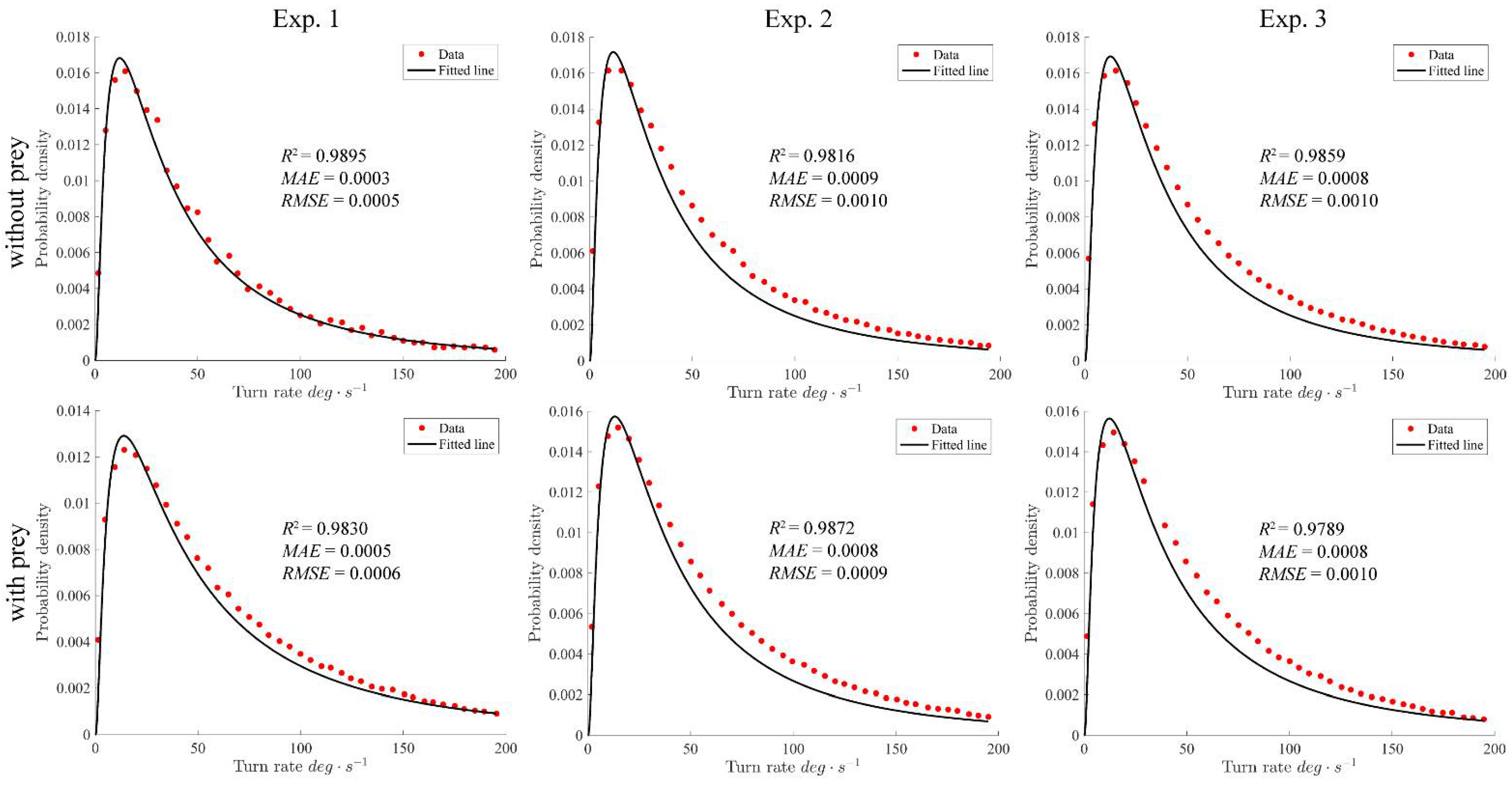
The distribution of the turning rate was fitted to the heavy-tailed distribution, specifically, the log-normal distribution (Figure 2). The fitting results showed extremely high R² ranging from 0.9789 to 0.9895, and low MAE ranging from 0.0003 to 0.0009 and RMSE ranging from 0.0005 to 0.0010 (Figure 2). The average value of turning rate ($\mu$) increased after the addition of food source, for both the situations of adding prey cells and cell-free filtrate (Table 1; Figure 2). The rate of increase is more than 3 times higher in the case of adding prey cells (7.56%), compared to that of adding the cell-free filtrate (2.32%). The value $\sigma$ in the equation of log-normal distribution represents the degree of randomness, with higher $\sigma$ value showing heavier tails in the distribution and higher randomness in the parameter examined. After addition of food sources, the $\sigma$ values for both situations (adding prey cells or cell-free filtrate) were higher, reflecting the increased randomness of turning rate in the dinoflagellate O. marina. Interestingly, similar to the average value ($\mu$), the increasing rate of $\sigma$ value is also higher in the case of adding prey cells (5.72%) as compared to adding cell-free filtrate (1.07%).

4.2. Swimming Speed

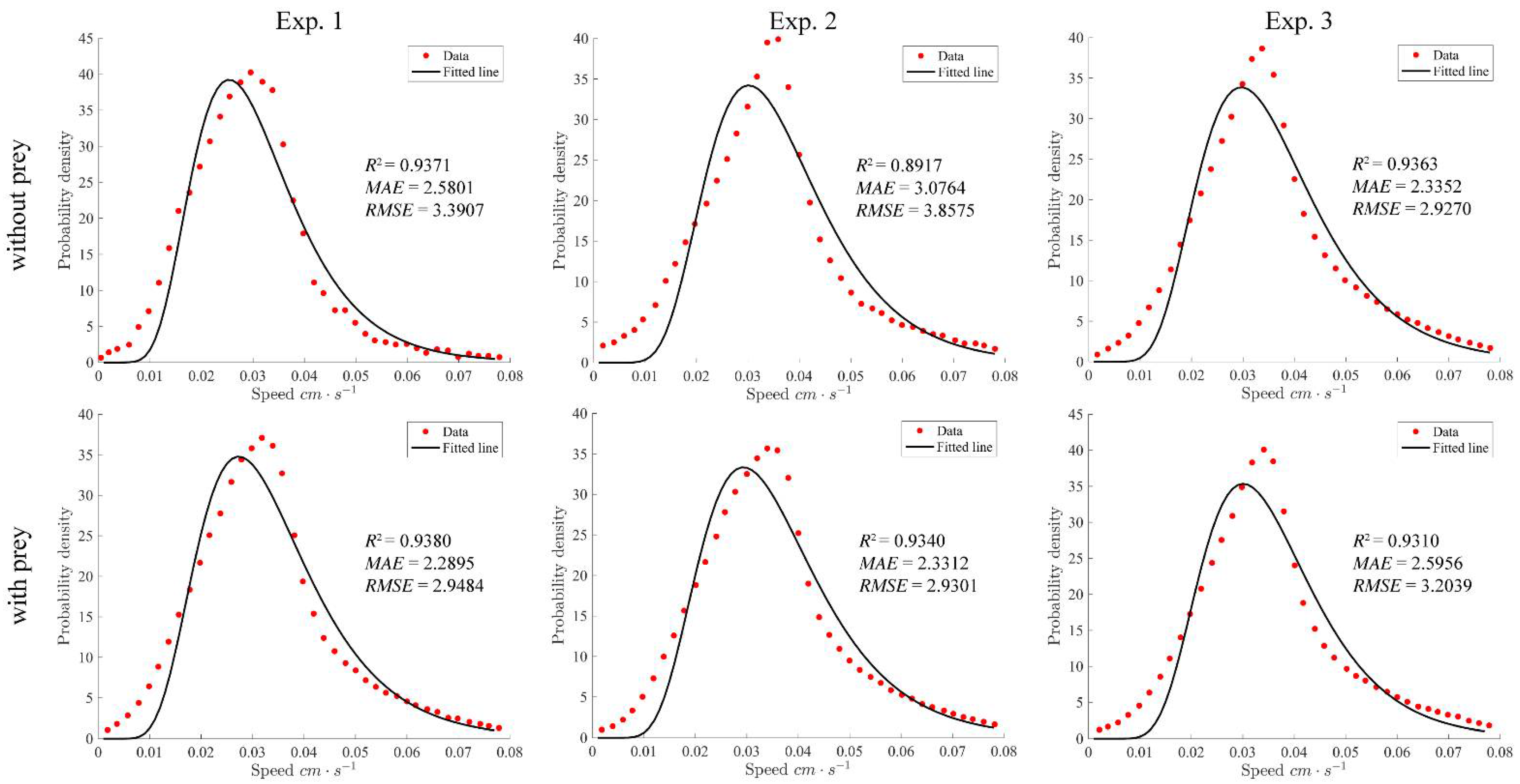
The fat tail was then examined in the distribution of swimming speed, by fitting to the log-normal distribution (Figure 3). The high R² ranging from 0.8917 to 0.9380, and low MAE ranging from 2.2895 to 3.0764 and RMSE ranging from 2.9270 to 3.8575 showed that the fits are quite robust (Figure 3). Given that the values are negative, the expected values and the variances were compared then (Table 2). The expected value $E\left(X\right)$ of swimming speed showed a difference in responses to the addition of prey cells and cell-free filtrate, i.e., the expected value of swimming speed increased from 0.03127 to 0.03428 cm s⁻¹ after adding the prey cells, which is 109.63% of the original speed. However, insignificantly decreasing was found for the case adding cell-free filtrate. Again, after the addition of food sources (adding prey cells), the variance $var\left(X\right)$ increased, reflecting higher randomness in the swimming speed for O. marina. However, the variance remains stable after the addition of cell-free filtrate.

4.3. Swimming Speeds during the Peak and Post-Peak Phases

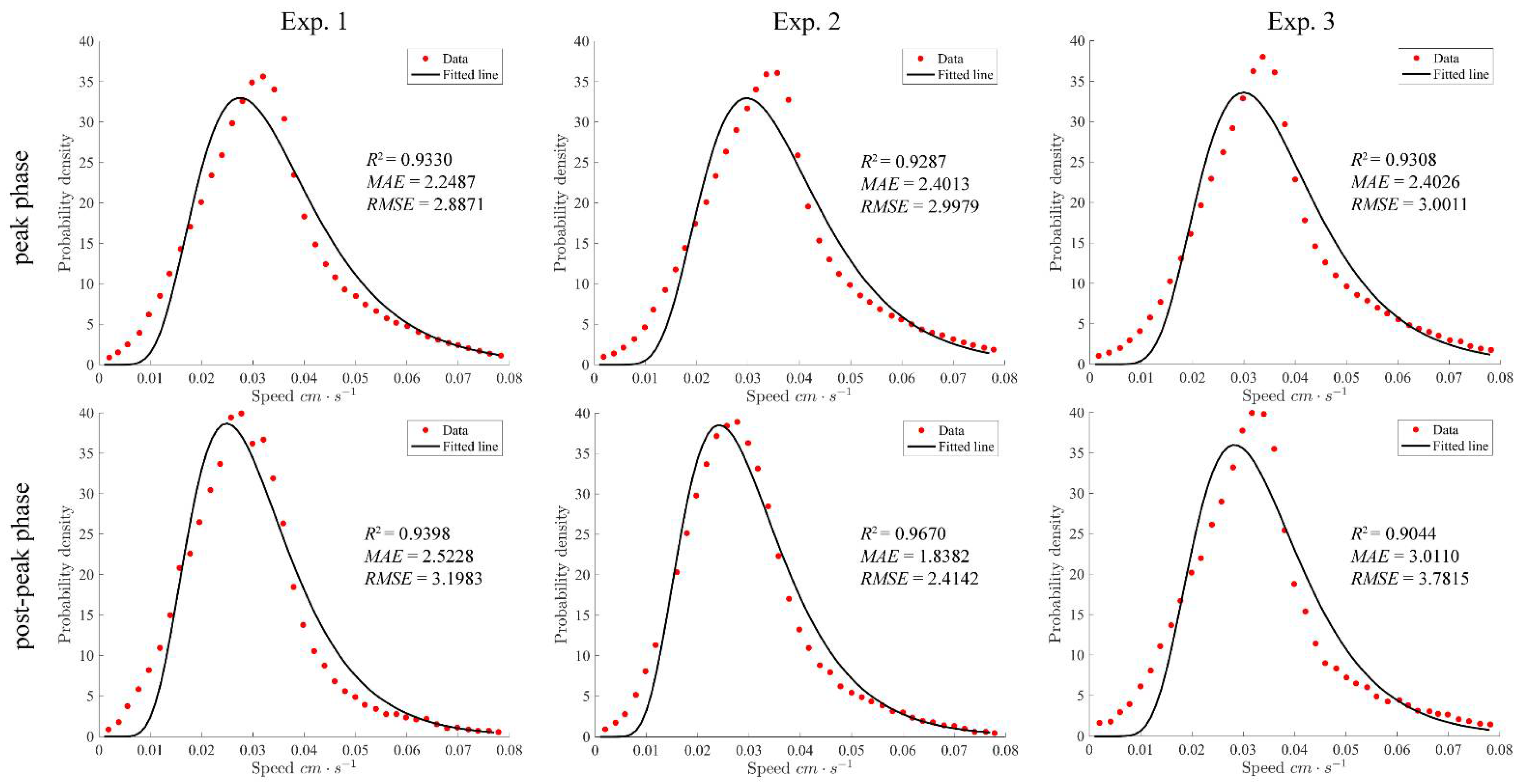
In all three experiments, after introduction of food sources, a rapid peak aggregation phase was found in relative abundance of the predator O. marina, followed by a post peak aggregation phase. The swimming speeds were higher in the peak phase, comparing to post-peak phase for both situations in terms of the expected values (Table 2, Figure 4). At the same time, the randomness of speed distribution increased after adding food sources and remained high in the peak phase. However, in the post-peak phase it (variance value) returned to normal, which is similar to the variance value before food addition.

4.4. Run Lengths

Fat tails were found in the distribution of run lengths as showed in the fits to the log-normal distribution (Figure 5), with high R² ranging from 0.9706 to 0.9834, and low MAE ranging from 1.4372 to 1.6524 and RMSE ranging from 1.8181 to 2.2128. The expected values and variances both slightly decreased after the addition of prey cells and cell-free filtrate (Table 2; Figure 5), reflecting better consistency in the run lengths of O. marina.

4.5. Path Curvature

Extremely high R² ranging from 0.9963 to 0.9996, and low MAE ranging from 0.0001 to 0.0003 and RMSE ranging from 0.0001 to 0.0003, showed clear existence of fat tails in the distribution of path curvatures (Figure 6). The value $\mu$ and $\sigma$ both increased after the addition of prey cells and cell-free filtrate (Table 1), as well as the expected values and variances (Table 2), reflecting less consistency and higher average value for the path curvatures of O. marina.

5. Discussion

5.1. The Known Knowns

Fat tails were observed to exist in the movement patterns of O. marina without and with the positive stimulations (food supply). The heavy tail distribution has been previously found in the movement patterns of a wide range of animal species [19], habituated in diverse environment from terrestrial (i.e., wandering albatrosses [20]) to intertidal and marine (i.e., gastropod [20], sea stars [19], calanoid copepod [22]). This scale-free random movements are considered to benefit the adaption of entire population to scarcity in fragmented ecosystems [24] and to enhance the predator’s encounter rate to prey [6].

The changes of movement patterns of O. marina to food supply were revealed by fitting the probability density values of the movement parameters to log-normal distribution formula. Results showed that after adding food resources, the turning angle increased after food supplied, but its randomness also increased. At the same time, the swimming speed became more disordered. The path curvature, therefore, increased in both the average value and the degree of disorder. The phenomenon of changes in the expected values for the indicators (turning rates, swimming speed and path curvature) were the same as the findings by direct observation of the difference between the probability density values before and after food supply [5]. Moreover, the analysis on the heavy tails indicated that the phytoplankton cells were using a random strategy to search for food, which was consistent with the theoretical calculations and numerical simulations [2,4,12]. In general, the changes in the movement patterns are larger when supplied by the direct prey cells, comparing to cell-free filtrate. Therefore, the adding of prey cells would trigger a stronger response in the phytoplankton population strategy to food sources.

5.2. The Known Unknowns

Although fat tails may exist in the swimming behavior and movement patterns of broader set of phytoplankton species, there are still many unknowns in this topic due to the limited experimental observations and data availability. For example, Laboratory observations on the well-known HABs forming species—Microsystis aeruginosa, which caused severe blooming all around the world [31,32,33,34,35], is still lacking. It will be interesting to investigate these HABs forming species and dig into the mechanisms from the perspective of movement-based ecological theories. Secondly, the actual phytoplankton movements are happening in a three-dimensional environment. Therefore, the 3D digital video capture system are needed to document the three-dimensional paths of phytoplankton [6,22]. Additionally, the following data process and analysis should also consider the three-dimension for better unrevealing the movement patterns. Finally, an important issue is how to link the randomness degree of movement patterns to the ecological behaviors of phytoplankton. So far, we have already known that the scale-free random movements support a sustainable balance between patch exploitation and regeneration over wide ranges of demographic rates [24]. However, a knowledge gap remains in explanation for the changes in movement patterns to various ecological and environmental factors in both positive and negative manners, e.g., the movement pattern of H. akashiwo in response to the turbulence [15,16].

5.3. The Unknown Unknowns

A major “unknown unknowns” concerns the movement patterns of small-size phytoplankton, although some of the picoplankton species (such as Prochlorococcus) are not motile. These tiny photosynthetic microorganisms, so-called picoplankton (diameter: 0.3–3 μm) and nanophytoplankton (3–20 μm), are at the base of the food web in many marine ecosystems and raised up attention world widely [36,37]. They play a ubiquitous and principal role in phytoplankton biomass and make an important contribution to primary production in the oceanic and freshwater ecosystem [36,37]. However, due to the limited resolution of the lens in a video camera system, the swimming behavior of small-size phytoplankton are not possible to be documented. By now, the two investigated phytoplankton by the video camera system are relatively big in diameter. For instance, the size of H. akashiwo is from 15 to 20 μm [38], which could be considered as a “giant” in the nanophytoplankton kingdom. Additionally, the other phytoplankton with movement traces documented (Oxyrrhis marina) ranges from 15 to 40 μm [39]. Since the picoplankton and nanophytoplankton are extremely small particles, and the physical characters of particles in such a scale could vary a lot. Unfortunately, we have no clear clue of how their swimming behavior and movement patterns would be, and, whether these patterns will follow the heavy tail distribution or a more complicated form. It is noteworthy that the 3D tracking method for E. coli to observe its tactic behavior has been conducted by microscopy since the 1970s [40]. Therefore, this “unknown unknown” will be better framed in the future, with the continuing development and adoption of innovative experiments. With improved resolution and precision, we are expected to make progress in our understanding by observing these small particles and making measurements that would not previously have been possible.

5.4. Fractal and Fractional Characteristics of Movement Patterns of Phytoplankton

A major outcome of the current study is that the movement pattern of O. marina can be fitted to log-normal distribution formula, a heavy-tailed distribution function described in Section 2. With this heavy-tailed distribution characteristics, it can be concluded that the movement series of O. marina can be also characterized by long-range dependence, fractal dimension, self-similarities and fractal-order, more detailed theory information can be found in Appendix A.

5.5. Prospect

As discussion in Section 5.4, future work could focus on exploring the fractal properties of the phytoplankton movement patterns and it can help gain more knowledge of the phytoplankton movement. Moreover, these theories can be also applied in exploring the characteristics of chlorophyll a concentration (served as biomass of phytoplankton) in waters [7,8,41].

6. Conclusions

In this paper, we employed log-normal distribution formula to fit the movements of the phytoplankton O. marina without and with positive (food supply) stimulations from existing data in the literature [5]. Fat tails were observed in the movement patterns of O. marina in terms of turning rates, swimming speed, peak speed, run length and path curvature). Specifically, with food supply stimulations, the O. marina will behavior in larger turning rate, swimming speed and path curvature, but smaller peak speed and run length, which make up the searching strategy for food. Mathematically, phytoplankton movement patterns have the property of long-range dependence, local self-similarity and a system of fractional-order by following the heavy tail distribution of the probability density values of the movement parameters.

References

1. Hays, G.C.; Richardson, A.J.; Robinson, C. Climate change and marine plankton. Trends Ecol. Evol. 2005, 20, 337–344. [Google Scholar] [CrossRef] [PubMed]
2. Levandowsky, M.; Klafter, J.; White, B. Swimming behavior and chemosensory responses in the protistan microzooplankton as a function of the hydrodynamic regime. Bull. Mar. Sci. 1988, 43, 758–763. [Google Scholar]
3. Menden-Deuer, S. Inherent high correlation of individual motility enhances population dispersal in a heterotrophic, planktonic protist. PLoS Comput. Biol. 2010, 6, e1000942. [Google Scholar] [CrossRef] [PubMed] [Green Version]
4. Visser, A.W. Lagrangian modelling of plankton motion: From deceptively simple random walks to Fokker-Planck and back again. J. Mar. Syst. 2008, 70, 287–299. [Google Scholar] [CrossRef]
5. Menden-Deuer, S.; Grunbaum, D. Individual foraging behaviors and population distributions of a planktonic predator aggregating to phytoplankton thin layers. Limnol. Oceanogr. 2006, 51, 109–116. [Google Scholar] [CrossRef] [Green Version]
6. Bartumeus, F.; Peters, F.; Pueyo, S.; Marrasé, C.; Catalan, J. Helical Lévy walks: Adjusting searching statistics to resource availability in microzooplankton. Proc. Natl. Acad. Sci. USA 2003, 100, 12771–12775. [Google Scholar] [CrossRef] [Green Version]
7. Xiao, X.; He, J.; Yu, Y.; Cazelles, B.; Li, M.; Jiang, Q.; Xu, C. Teleconnection between phytoplankton dynamics in north temperate lakes and global climatic oscillation by time-frequency analysis. Water Res. 2019, 154, 267–276. [Google Scholar] [CrossRef]
8. Xiao, X.; He, J.; Huang, H.; Miller, T.R.; Christakos, G.; Reichwaldt, E.S.; Ghadouani, A.; Lin, S.; Xu, X.; Shi, J. A novel single-parameter approach for forecasting algal blooms. Water Res. 2017, 108, 222–231. [Google Scholar] [CrossRef]
9. Xiao, X.; Agusti, S.; Pan, Y.; Yu, Y.; Li, K.; Wu, J.; Duarte, C.M. Warming amplifies the frequency of Harmful Algal Blooms with eutrophication in Chinese coastal waters. Environ. Sci. Technol. 2019, 53, 13031–13041. [Google Scholar] [CrossRef]
10. Xu, C.; Ge, Z.; Li, C.; Wan, F.; Xiao, X. Inhibition of harmful algae Phaeocystis globosa and Prorocentrum donghaiense by extracts of coastal invasive plant Spartina alterniflora. Sci. Total Environ. 2019, 696, 133930. [Google Scholar] [CrossRef]
11. Xiao, X.; Li, C.; Huang, H.; Lee, Y.P. Inhibition effect of natural flavonoids on red tide alga Phaeocystis globosa and its quantitative structure-activity relationship. Environ. Sci. Pollut. Res. 2019, 26, 23763–23776. [Google Scholar] [CrossRef] [PubMed]
12. Liu, G.; Janowitz, G.S.; Kamykowski, D. Influence of environmental nutrient conditions on Gymnodinium breve (Dinophyceae) population dynamics: A numerical study. Mar. Ecol. Prog. Ser. 2001, 213, 13–37. [Google Scholar] [CrossRef] [Green Version]
13. Kim, H.; Spivack, A.J.; Menden-Deuer, S. pH alters the swimming behaviors of the raphidophyte Heterosigma akashiwo: Implications for bloom formation in an acidified ocean. Harmful Algae 2013, 26, 1–11. [Google Scholar] [CrossRef]
14. Harvey, E.L.; Menden-Deuer, S. Avoidance, movement, and mortality: The interactions between a protistan grazer and Heterosigma akashiwo, a harmful algal bloom species. Limnol. Oceanogr. 2011, 56, 371–378. [Google Scholar] [CrossRef] [Green Version]
15. Sengupta, A.; Carrara, F.; Stocker, R. Phytoplankton can actively diversify their migration strategy in response to turbulent cues. Nature 2017, 543, 7646. [Google Scholar] [CrossRef]
16. Carrara, F.; Sengupta, A.; Behrendt, L.; Vardi, A.; Stocker, R. Bistability in oxidative stress response determines the migration behavior of phytoplankton in turbulence. Proc. Natl. Acad. Sci. USA 2021, 118. [Google Scholar] [CrossRef] [PubMed]
17. An, X.; Li, X.; Gong, C. Research progress on ecological characteristics of Oxyrrhis marina. J. Shanghai Ocean Univ. 2013, 22, 364–369. [Google Scholar]
18. Krishnamurthy, D.; Li, H.; Du Rey, F.B.; Cambournac, P.; Larson, A.G.; Li, E.; Prakash, M. Scale-free vertical tracking microscopy. Nat. Methods 2020, 17, 1040–1051. [Google Scholar] [CrossRef]
19. Lohmann, A.C.; Evangelista, D.; Waldrop, L.D.; Mah, C.L.; Hedrick, T.L. Covering Ground: Movement Patterns and Random Walk Behavior in Aquilonastra anomala Sea Stars. Biol. Bull. 2016, 231, 130–141. [Google Scholar] [CrossRef]
20. Seuront, L.; Duponchel, A.C.; Chapperon, C. Heavy-tailed distributions in the intermittent motion behaviour of the intertidal gastropod Littorina littorea. Phys. A Stat. Mech. Its Appl. 2007, 385, 573–582. [Google Scholar] [CrossRef]
21. Viswanathan, G.M.; Afanasyev, V.; Buldyrev, S.; Murphy, E.; Prince, P.; Stanley, H.E. Lévy flight search patterns of wandering albatrosses. Nature 1996, 381, 413. [Google Scholar] [CrossRef]
22. Michalec, F.G.; Ka, S.; Holzner, M.; Souissi, S.; Ianora, A.; Hwang, J.S. Changes in the swimming behavior of Pseudodiaptomus annandalei (Copepoda, Calanoida) adults exposed to the diatom toxin 2-trans, 4-trans decadienal. Harmful Algae 2013, 30, 56–64. [Google Scholar] [CrossRef]
23. Huo, H.; He, R.; Zhang, R.; Yuan, J. Swimming Escherichia coli Cells Explore the Environment by Lévy Walk. Appl. Environ. Microbiol. 2021, 87. [Google Scholar] [CrossRef]
24. Dannemann, T.; Boyer, D.; Miramontes, O. Lévy flight movements prevent extinctions and maximize population abundances in fragile Lotka–Volterra systems. Proc. Natl. Acad. Sci. USA 2018, 115, 3794–3799. [Google Scholar] [CrossRef] [PubMed] [Green Version]
25. Ghanbari, B.; Günerhan, H.; Srivastava, H.M. An application of the Atangana-Baleanu fractional derivative in mathematical biology: A three-species predator-prey model. Chaos Solitons Fractals 2020, 138, 109910. [Google Scholar] [CrossRef]
26. Ghanbari, B.; Djilali, S. Mathematical analysis of a fractional-order predator-prey model with prey social behavior and infection developed in predator population. Chaos Solitons Fractals 2020, 138, 109960. [Google Scholar] [CrossRef]
27. Kumar, S.; Kumar, R.; Cattani, C.; Samet, B. Chaotic behaviour of fractional predator-prey dynamical system. Chaos Solitons Fractals 2020, 135, 109811. [Google Scholar] [CrossRef]
28. Yavuz, M.; Sene, N. Stability Analysis and Numerical Computation of the Fractional Predator–Prey Model with the Harvesting Rate. Fractal Fract. 2020, 4, 35. [Google Scholar] [CrossRef]
29. Owolabi, K.M. Dynamical behaviour of fractional-order predator-prey system of Holling-type. Discret. Contin. Dyn. Syst. S 2020, 13, 823–834. [Google Scholar] [CrossRef] [Green Version]
30. Bonyah, E.; Atangana, A.; Elsadany, A.A. A fractional model for predator-prey with omnivore. Chaos Interdiscip. J. Nonlinear Sci. 2019, 29, 013136. [Google Scholar] [CrossRef]
31. Yu, S.; Li, C.; Xu, C.; Effiong, K.; Xiao, X. Understanding the inhibitory mechanism of antialgal allelochemical flavonoids from genetic variations: Photosynthesis, toxin synthesis and nutrient utility. Ecotoxicol. Environ. Saf. 2019, 177, 18–24. [Google Scholar] [CrossRef] [PubMed]
32. Wu, Y.; Wang, F.; Xiao, X.; Liu, J.; Wu, C.; Chen, H.; Kerr, P.; Shurin, J. Seasonal changes in phosphorus competition and allelopathy of a benthic microbial assembly facilitate prevention of cyanobacterial blooms. Environ. Microbiol. 2017, 19, 2483–2494. [Google Scholar] [CrossRef] [PubMed]
33. Huang, H.; Xiao, X.; Lin, F.; Grossart, H.-P.; Nie, Z.; Sun, L.; Xu, C.; Shi, J. Continuous-release beads of natural allelochemicals for the long-term control of cyanobacterial growth: Preparation, release dynamics and inhibitory effects. Water Res. 2016, 95, 113–123. [Google Scholar] [CrossRef]
34. Huang, H.; Xiao, X.; Ghadouani, A.; Wu, J.; Nie, Z.; Peng, C.; Xu, X.; Shi, J. Effects of Natural Flavonoids on Photosynthetic Activity and Cell Integrity in Microcystis aeruginosa. Toxins 2015, 7, 66–80. [Google Scholar] [CrossRef] [PubMed] [Green Version]
35. Xiao, X.; Huang, H.M.; Ge, Z.W.; Rounge, T.B.; Shi, J.Y.; Xu, X.H.; Li, R.; Chen, Y. A pair of chiral flavonolignans as novel anti-cyanobacterial allelochemicals derived from barley straw (Hordeum vulgare): Characterization and comparison of their anti-cyanobacterial activities. Environ. Microbiol. 2014, 16, 1238–1251. [Google Scholar] [CrossRef]
36. Blanc-Mathieu, R.; Krasovec, M.; Hebrard, M.; Yau, S.; Desgranges, E.; Martin, J.; Schackwitz, W.; Kuo, A.; Salin, G.; Donnadieu, C.; et al. Population genomics of picophytoplankton unveils novel chromosome hypervariability. Sci. Adv. 2017, 3, e1700239. [Google Scholar] [CrossRef] [Green Version]
37. Guo, R.; Liang, Y.; Xin, Y.; Wang, L.; Cao, C.; Xie, R.; Zhang, C.; Tian, J.; Zhang, Y. Insight into the pico-and nano-phytoplankton communities in the deepest biosphere, the Mariana Trench. Front. Microbiol. 2018, 9, 2289. [Google Scholar] [CrossRef] [Green Version]
38. Khan, S.; Arakawa, O.; Onoue, Y. Neurotoxins in a toxic red tide of Heterosigma akashiwo (Raphidophyceae) in Kagoshima Bay, Japan. Aquac. Res. 1997, 28, 9–14. [Google Scholar] [CrossRef]
39. Hansen, F.C.; Witte, H.J.; Passarge, J. Grazing in the heterotrophic dinoflagellate Oxyrrhis marina: Size selectivity and preference for calcified Emiliania huxleyi cells. J. Aquat. Microb. Ecol. 1996, 10, 307–313. [Google Scholar] [CrossRef]
40. Berg, H.C.; Brown, D.A. Chemotaxis in Escherichia coli analysed by Three-dimensional Tracking. Nat. Cell Biol. 1972, 239, 500–504. [Google Scholar] [CrossRef]
41. He, J.; Chen, Y.; Wu, J.; Stow, D.; Christakos, G. Space-Time Chlorophyll-a Retrieval in Optically Complex Waters that Accounts for Remote Sensing and Modeling Uncertainties and Improves Remote Estimation Accuracy. Water Res. 2020, 171, 1–17. [Google Scholar] [CrossRef]
42. Samorodnitsky, G.; Taqqu, M.S. Stable Non-Gaussian Random Processes: Stochastic Models with Infinite Variance; Chapman and Hall: New York, NY, USA, 1994. [Google Scholar]
43. Adler, R.J.; Feldman, R.E.; Taqqu, M.S. (Eds.) A Practical Guide to Heavy Tails: Statistical Techniques and Applications; Birkhäuser: Boston, MA, USA, 1998. [Google Scholar]
44. Li, M. Fractal time series—A tutorial review. Math. Probl. Eng. 2010, 2010, 157264. [Google Scholar] [CrossRef]
45. Fontugne, R.; Abry, P.; Fukuda, K.; Veitch, D.; Cho, K.; Borgnat, P.; Wendt, H. Scaling in internet traffic: A 14 year and 3 day longitudinal study, with multiscale analyses and random projections. IEEE/ACM Trans. Netw. 2017, 25, 2152–2165. [Google Scholar] [CrossRef] [Green Version]
46. Mandelbrot, B.B.; van Ness, J.W. Fractional Brownian motions, fractional noises and applications. SIAM Rev. 1968, 10, 422–437. [Google Scholar] [CrossRef]
47. Mandelbrot, B.B. Gaussian Self-Affinity and Fractals; Springer: Berlin/Heidelberg, Germany, 2001. [Google Scholar]
48. Mandelbrot, B.B. Fast fractional Gaussian noise generator. Water Resour. Res. 1971, 7, 543–553. [Google Scholar] [CrossRef]
49. Li, M. Record length requirement of long-range dependent teletraffic. Physics A 2017, 472, 164–187. [Google Scholar] [CrossRef]
50. Davies, S.; Hall, P. Fractal analysis of surface roughness by using spatial data. J. R. Stat. Soc. Ser. B 1999, 61, 3–37. [Google Scholar] [CrossRef]
51. Li, M. Generation of teletraffic of generalized Cauchy type. Phys. Scr. 2010, 81, 025007. [Google Scholar] [CrossRef]
52. Li, M.; Sun, X.; Xiao, X. Revisiting fractional Gaussian noise. Physics A 2019, 514, 56–62. [Google Scholar] [CrossRef]
53. Li, M. Multi-fractional generalized Cauchy process and its application to teletraffic. Physics A 2020, 550, 123982. [Google Scholar] [CrossRef]
Figure 1. Comparison of the (a) expectation value and (b) variance between log-normal distribution and normal distribution. In (a), σ = 0.6 ; in (b), μ = 1 .
Fractalfract 05 00049 g001
Figure 2. Fat tails in the frequency distributions of turning rates of O. marina before (top) and after (bottom) the introduction of a layer of I. galbana prey cells in three separate experiments (Exp. 1 with either direct addition of the prey alga; Exp. 2&3 with cell-free filtrate). The red dots: original data; black line: fitted curve using log-normal distribution formula.
Fractalfract 05 00049 g002
Figure 3. Fat tails in the frequency distributions of swimming speeds of O. marina before (top) and after (bottom) the introduction of a prey layer (Exp. 1 with either direct addition of the prey alga; Exp. 2&3 with cell-free filtrate) The red dots: original data; black line: fitted curve using log-normal distribution formula.
Fractalfract 05 00049 g003
Figure 4. Fat tails in the frequency distributions of swimming speeds of O. marina during the peak (top) and post-peak (bottom) aggregation phases (Exp. 1 with either direct addition of the prey alga; Exp. 2&3 with cell-free filtrate). The red dots: original data; black line: fitted curve using Log-normal distribution formula.
Fractalfract 05 00049 g004
Figure 5. Fat tails in the frequency distributions of run lengths of O. marina before (top) and after (bottom) the introduction of a phytoplankton thin layer (Exp. 1 with either direct addition of the prey alga; Exp. 2&3 with cell-free filtrate). The red dots: original data; black line: fitted curve using log-normal distribution formula.
Fractalfract 05 00049 g005
Figure 6. Fat tails in the frequency distributions of path curvature of O. marina before (top) and after (bottom) the introduction of a phytoplankton thin layer (Exp. 1 with either direct addition of the prey alga; Exp. 2&3 with cell-free filtrate). The red dots: original data; black line: fitted curve using log-normal distribution formula.
Fractalfract 05 00049 g006