Fractal Flow Characterization of Multiscale Fracture Networks in Hydraulically Fractured Dolomite Reservoirs Using Rate Transient Analysis

Abstract

Conventional Rate Transient Analysis (RTA) models, based on homogeneous fracture assumptions, are inadequate for characterizing flow in complex fracture networks of heterogeneous unconventional reservoirs. This study develops a fractal-based RTA (FD-RTA) workflow integrating lithofacies analysis, microseismic fracture interpretation, and post-fracturing production data from the Yingxiongling shale oil field in the Q’aidam Basin. The workflow is applied to eight horizontal wells completed in layered and laminated dolomites. Results show that the two lithofacies exhibit distinct fractal flow behaviors. Layered dolomite tends to develop preferential flow pathways, characterized by rapid initial depletion followed by declining supply capacity, with the half-flow dimension (δ) decreasing from 0.299 to 0.074 during production. Laminated dolomite displays stronger fracture-matrix interaction and sustained production performance, with δ increasing from 0.469 to 0.678 as multi-scale fractures are progressively activated. The FD-RTA workflow effectively links fracture complexity with production behavior, providing a dynamic characterization tool for evaluating hydraulic fracturing effectiveness in shale oil reservoirs.

1. Introduction

Shale oil constitutes a major component of global hydrocarbon resources [1,2,3]. In recent years, low-permeability, low-porosity unconventional carbonate reservoirs with complex fracture systems have become key targets for reserve growth and production [4,5,6]. Hydraulic fracturing is essential for enhancing permeability in such reservoirs. The spatial architecture of fracture networks governs both the stimulated reservoir volume and fluid transport pathways, ultimately determining long-term productivity. Accurate evaluation of post-fracturing effective flow space and its dynamic evolution therefore remains a critical challenge in shale reservoir development [7,8,9].

Microseismic monitoring and production performance analysis are the primary techniques for evaluating fracturing effectiveness. Microseismic mapping describes fracture propagation geometry and spatial distribution, while production response reflects the effective fracture space and fluid transport capacity actually contributing to flow [10,11]. However, no simple one-to-one correspondence exists between fracture geometric complexity and production behavior. Establishing quantitative links among fracture architecture, effective flow space, and production dynamics remains a key challenge in characterizing complex fractured reservoirs.

Rate Transient Analysis (RTA) is widely applied to evaluate flow characteristics and fracturing effectiveness in unconventional reservoirs [12]. The early Arps decline model was extensively used for production forecasting and reserve estimation [13]. Subsequently, Blasingame, Agarwal-Gardner, and others developed rate-normalized pressure and material balance time methods, improving parameter interpretation under variable production conditions [14]. For multi-stage fractured horizontal wells, linear flow, bilinear flow, and multi-fracture analytical models have been proposed to describe fracture-controlled flow regimes and reservoir response [12,15,16]. These methods have proven effective in shale gas and tight oil development and form the theoretical basis for unconventional reservoir evaluation [17]. Nevertheless, conventional RTA models typically rely on idealized fracture geometries. Actual fracture networks, shaped by natural fractures, bedding planes, and stress heterogeneity, involve multi-scale fractures that contribute simultaneously to fluid transport. Pressure propagation consequently deviates from classical diffusion, often exhibiting anomalous diffusion and transitional flow behavior [18].

Fractal theory, introduced by Mandelbrot, describes self-similar and scale-invariant complex structures in nature [19]. Given the inherently scale-distributed characteristics of natural porous media and fracture networks, fractal methods have been increasingly applied to pore-structure characterization, permeability prediction, and fracture-network description [20]. Fracture length, aperture, and spatial distribution typically follow power-law statistics, making fractal geometry a suitable mathematical framework for characterizing complex fracture networks [21]. However, application of fractal flow theory to strongly heterogeneous carbonate reservoirs remains limited, and the relationships among fractal parameters, fracture complexity, effective flow space, and actual production response lack systematic investigation. Integrating fractal-based dynamic analysis with microseismic interpretation and lithofacies characterization may therefore bridge the scale gap between fracture architecture and production behavior [22,23]. This study targets hydraulically fractured horizontal wells in the Yingxiongling shale oil field of the Q’aidam Basin, developing an FD-RTA workflow based on fractal flow theory, coupled with microseismic interpretation, production data, and lithofacies classification, to investigate dynamic drainage mechanisms in complex fracture systems.

2. Geological Setting and Data

2.1. Geological Setting and Reservoir Characteristics

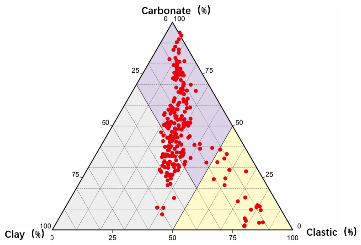
The Yingxiongling shale oil play is situated in the western Q’aidam Basin, forming an integral part of the Paleogene–Neogene petroleum system in the western Q’aidam region. The target interval is the upper member of the Lower Ganchaigou Formation (E_2–3xg²), a saline lacustrine mixed sedimentary system. Unlike typical continental mudstone–shale reservoirs, this interval exhibits interbedded argillaceous and carbonate lithologies (Figure 1) [24].

Controlled by fluctuations in the depositional environment, lake-level variations, and salinity changes, the reservoir displays strong vertical cyclicity, with marked differences in mineral composition, rock fabric, and pore types among layers. Dolomite-rich intervals constitute the most significant reservoir lithofacies in the study area.

2.2. Reservoir Heterogeneity

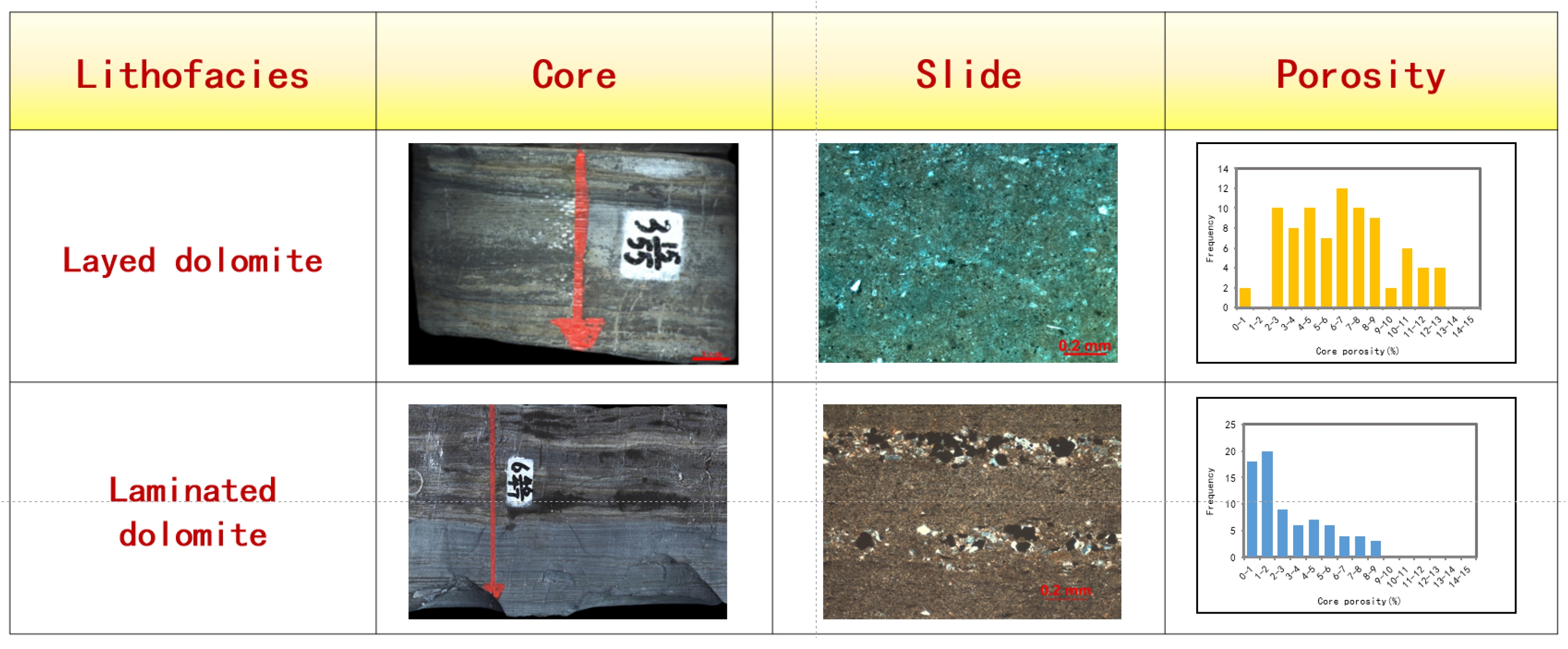
Based on mineral composition, depositional texture, and rock fabric, the dolomite reservoir in the study area is classified into two main lithofacies: layered dolomite and laminated dolomite (Figure 2).

Layered dolomite is grayish–white to dark gray in color, with dolomite content ranging from 40% to 70% and low terrigenous clastic content. Individual bed thickness generally exceeds 1 cm. The dolomite is uniformly mixed with argillaceous components, with localized enrichment of dolomite in layered patterns. Core and thin-section observations indicate that this lithofacies is relatively homogeneous in rock fabric, with intercrystallite pores as the dominant pore type. Pore distribution is relatively concentrated, and porosity is generally stable.

Laminated dolomite is gray to dark gray in color, with dolomite content generally exceeding 50% and low terrigenous clastic content. Core and thin-section images reveal alternating light and dark fine laminae, with dolomite laminae (lighter in color) interbedded with clay-rich laminae. Individual lamina thickness is less than 1 cm. Due to the development of laminated structures, laminated dolomite exhibits more dispersed pore distribution and relatively lower porosity compared to layered dolomite.

As previously reported by the authors, the mechanical differences between the two lithofacies originate from their distinct depositional fabrics. Layered dolomite is structurally homogeneous, with poorly developed bedding and weak mechanical anisotropy; thus, hydraulic fractures propagate unidirectionally along the maximum principal stress direction. In contrast, laminated dolomite contains densely spaced bedding planes, which serve as planes of mechanical weakness during hydraulic fracturing. When fractures encounter these bedding planes, they tend to deflect, branch, or open along the bedding, resulting in the formation of more complex fracture networks [25].

2.3. Hydraulic Fracturing and Production Data

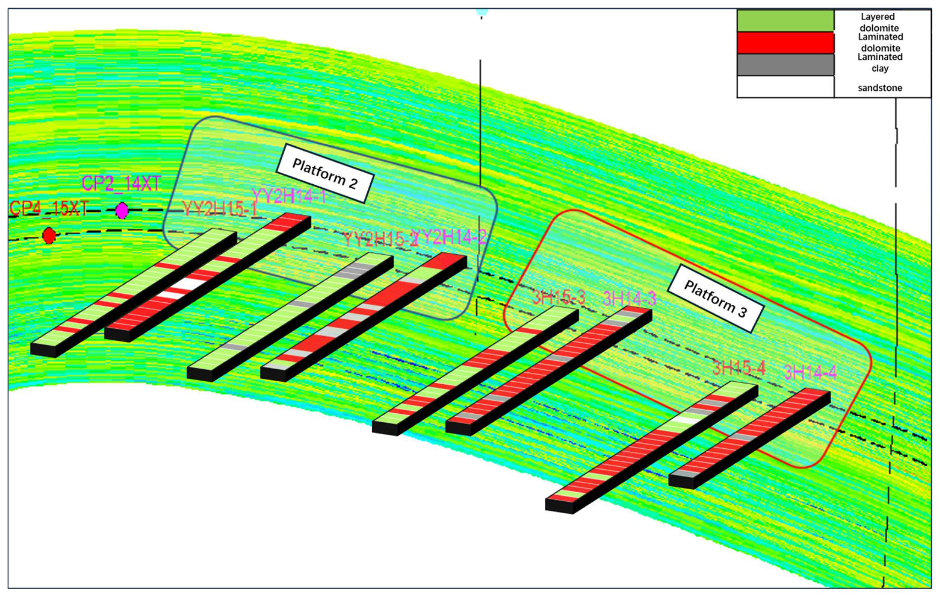
The study targets two pads, 2H and 3H, located in the structural high of the medium-sweet-spot area, comprising eight horizontal wells. The two pads share similar structural settings and development conditions. The 2H pad is predominantly layered dolomite, whereas the 3H pad is primarily laminated dolomite (Figure 3).

2.3.1. Fracturing Treatment Parameters

Fracturing treatment parameters for each well are listed in

Table 1. The basic fracturing data of platform wells.

Well Name	Horizontal Section Length/m	Drilling Success Rate/%	Stage	Pump Rate/m3/min	Pump Volume/m3	Proppant Volume/m3	Fracturing Fluid Intensity/m3/m	Proppant Intensity/m3/m
2H14-1	1510	78.8	24	16	41,092	3918	27.21	2.59
2H14-2	1509	85.7	23	16	45,572	4443	30.20	2.94
2H15-1	1480	82.3	27	16	41,459	4162	28.01	2.81
2H15-2	1456	91.1	19	16	44,711	4634	30.71	3.18
3H14-3	1437	100	24	15.6	37,608	3994	26.80	2.85
3H14-4	1114	96.5	19	15.6	34,621	3641	29.00	3.05
3H15-3	1410	100	27	16	41,662	3960	28.38	2.7
3H15-4	1434	90.9	27	15.5	47,069	4327	31.72	2.92

. Horizontal section length ranges from 1114 to 1510 m, with 19 to 27 fracturing stages per well, a pump rate of 15.5 to 16 m³/min, injected fluid volume of 34,621 to 47,069 m³, and proppant volume of 3641 to 4634 m³. The two pads exhibit generally similar treatment scales, yet their microseismic responses differ markedly, indicating that fracture propagation behavior is primarily governed by lithofacies rather than engineering parameters.

2.3.2. Microseismic Monitoring and Fracture Interpretation

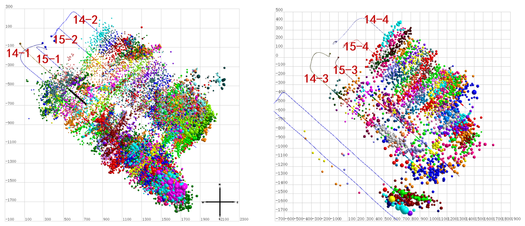
Microseismic monitoring records elastic wave signals generated by rock failure during fracturing through receivers deployed in offset wells and employs event location methods to determine fracture propagation geometry and spatial distribution (Figure 4) [10].

After normalizing for horizontal section length, asymmetric fracture propagation is observed in both pads. Based on microseismic inversion results, geometric parameters including fracture length, fracture width, fracture height, and stimulated reservoir volume (SRV) were obtained for each fractured stage to characterize hydraulic fracture geometry. To further evaluate fracture-network complexity, the b-value was calculated from the magnitude distribution of microseismic events using the Gutenberg–Richter frequency–magnitude relationship:

$$\mathit{log}N=a-bM$$

(1)

where $M$ is magnitude, N is the number of events, a reflects the level of seismic activity, and b describes the distribution of events across different magnitudes. A higher b value indicates a larger proportion of small-magnitude events, reflecting a higher degree of fracture branching during propagation.

Due to equipment malfunction during certain fracturing stages at the 3H pad, some stages lack valid monitoring data; fracture parameters and b values are therefore analyzed based on available stages. Recognizing that well-averaged values may mask stage-to-stage variations caused by localized lithofacies differences, this study adopts individual fracturing stages as statistical units. Stages are classified by lithofacies according to horizontal well trajectory and corresponding lithofacies interpretation at each stage location. Fracture length, width, height, SRV, and b value are then statistically compared across lithofacies types to evaluate differences in fracture geometry and complexity.

Microseismic results indicate that the two lithofacies exhibit similar dominant fracture dimensions—fracture length ranges from approximately 345 to 351 m, height ranges from 57 to 58 m, and width differs by less than 5%. However, laminated dolomite shows an approximately 8% higher SRV and nearly 15% higher b value compared to layered dolomite (

Table 2. Interpreted fracturing parameters from microseismic events.

Lithofacies	Fracture Length/m	Fracture Width/m	Fracture Height/m	SRV/104 m3	b-Value
Layered dolomite	345.2941	93.8235	58.4902	103.5412	1.4352
Laminated dolomite	351.1324	89.2794	57.47059	112.1676	1.6491

1. The SRV derived from microseismic interpretation (Stimulated Reservoir Volume, hereinafter referred to as SRV_geo) represents the geometric volume enclosed by the distribution of microseismic events during fracturing, with units of 10⁴ m³.

). Under comparable treatment conditions, laminated dolomite develops fracture systems with greater spatial complexity.

Overall, the microseismic results indicate that the differences between lithofacies are not primarily reflected in fracture dimensions but in the spatial organization and complexity of the fracture networks.

2.3.3. Production Data and Preprocessing

Production data from the eight wells from startup to 2026 were collected for FD-RTA analysis. The dataset includes the daily oil rate, daily liquid rate, water cut, cumulative production, and wellhead oil and casing pressures.

Multiple wells experienced shut-ins, workover operations, and production schedule adjustments during the production period. These non-reservoir disturbances introduce spurious signals on pressure-derivative plots and interfere with flow-regime identification. The following preprocessing steps were applied:

• Non-production events were flagged based on operation logs, and data segments within 3 to 5 days around each event were removed.
• The filtered production time series were normalized, with time reset to zero at production start and sorted by cumulative production days.
• Wellhead pressures were converted to bottomhole flowing pressures using a multiphase wellbore pressure-drop model incorporating the gas–oil ratio, water cut, and wellbore temperature gradient.

After preprocessing, the longest continuous stable production segment of each well was selected as the primary analysis window for FD-RTA inversion.

3. Methodology: Fractal-Based Rate Transient Analysis

3.1. Fractal Characterization of Multiscale Fracture Networks

Complex fracture networks are characterized by self-similarity in fracture length and spatial distribution. According to fractal theory, fracture population and length follow a power-law relationship:

$$N\left(l\right)=C_l{l}^{-D_f}$$

(2)

where $l$ is fracture length, $N\left(l\right)$ is the number of fractures with a length greater than $l$, and $C_l$ is the fracture size distribution coefficient. The fractal dimension ($D_f$) quantifies the space-filling capacity of the fracture network across scales. A higher $D_f$ indicates a greater proportion of small-scale fractures and more complex spatial distribution.

The half-flow dimension ($\delta =D_f/2$) is defined for subsequent flow modeling [26], with $\delta =0.5$ corresponding to linear flow, $\delta =1$ to radial flow, and $0.5<\delta <1$ to transitional fractal flow.

In rate transient analysis, the pressure-derivative curve exhibits a power-law relationship during the fractal flow regime, where the slope ($\alpha$) is related to $\delta$ [26,27]. In log–log coordinates, linear flow yields a derivative slope of 1/2, corresponding to $\delta =0.5$ and $D_f=1$. When the actual slope deviates from 1/2, $D_f=2(1-\alpha )$. For ideal radial flow, $D_f=2$; for ideal linear flow, $D_f=1$. In real complex fracture networks, $D_f$ falls between these two end-members.

3.2. Fractal Transient Flow Model

Conventional RTA models assume an integer-dimensional pressure propagation space, corresponding to linear flow (derivative slope of 1/2) and radial flow (slope of 0). In complex fracture networks, however, fractures are multi-scale and heterogeneously distributed, causing pressure propagation to deviate from classical diffusion, and the pressure-derivative curve often exhibits transitional slopes between 1/2 and 0.

For a single set of fractures of length $l$, the effective flow area is expressed as

$$d{A}_f=lwh,$$

(3)

where $w$ is the fracture width and $h$ is the effective fracture height.

According to the distribution of fracture length, the number of fractures between $l\sim l+dl$ is

$$dN={-D}_f{\displaystyle \frac{dN\left(l\right)}{dl}}dl,$$

(4)

where $N\left(l\right)$ is the cumulative number of fractures. Due to the $N\left(l\right)$ decreases as $l$ increases, its derivative is negative.

Therefore, the contributed effective flow area of the fracture is

$$d{A}_f=dN\cdot lwh.$$

(5)

Taking Equation (4) into Equation (5) yields

$$d{A}_f=C_{l}wh{l}^{1-D_f}dl.$$

(6)

Integrating over all fracture scales yields the total effective flow area of the fracture network:

$$A_f={\int }_{l_{min}}^{l_{max}}{C}_{l}wh{l}^{1-D_f}dl$$

(7)

Integrating yields

$$A_f={\displaystyle \frac{C_{l}wh}{2-D_f}}\left(l_{max}^{2-D_f}−l_{min}^{2-D_f}\right),$$

(8)

where $l_{max}$ and $l_{min}$ represent the maximum and minimum effective length in the fracture network, respectively.

Equation (8) shows that the effective flow area of a complex fracture network is governed by the fracture size distribution.

During post-fracturing production, as the pressure disturbance region progressively expands, the maximum fracture scale contributing to flow increases accordingly. Therefore,

$$l_{max}\approx r,$$

(9)

where r is the pressure propagation range.

When the pressure propagation range is far larger than the minimum fracture length, which is $r\gg l_{min}$, Equation (8) can be simplified as

$$A_f\left(r\right)\propto r^{2-D_f}.$$

(10)

Substituting the above relationship into Darcy’s law and the diffusivity equation yields the famous O’Shaughnessy–Procaccia equation for diffusion on fractals [28]:

$${\displaystyle \frac{\partial p}{\partial t}}=\eta {\displaystyle \frac{1}{r^{\delta -1}}}{\displaystyle \frac{\partial }{\partial r}}\left(r^{\delta -1}{\displaystyle \frac{\partial p}{\partial r}}\right),$$

(11)

where $p$ is reservoir pressure, $t$ is production time, $r$ is pressure propagation distance, $\eta$ is the coefficient of pressure propagation, and $\delta$ is the half-flow dimension.

In the stage of fractal flow, the bottomhole pressure derivative in log–log coordinates satisfies the following:

$$t{\displaystyle \frac{dp}{dt}}=m{t}^{1-\delta }$$

(12)

In other words, the pressure derivative appears as a straight line on the log–log plot, with a slope of $\alpha =1-\delta$. Thus, $\delta$ can be directly obtained from the slope of the measured curve:

$$\delta =1-\alpha$$

(13)

In practice, the slope (α) was determined by numerically computing $dp/dt$ from the measured bottomhole pressure data after smoothing, using only the data points within the intermediate-time linear-flow regime identified from the RNP diagnostic plots.

Since discrete pressure and production data cannot be directly correlated with continuous pressure propagation distance, Acuna introduced the Characteristic Flow Volume (CFV). CFV is defined as the pore volume from the fracture network to a given distance and can be directly calculated from production data. Unlike microseismic SRV, which reflects geometric fracture volume, CFV is derived from production response and represents the reservoir volume actually contributing to flow within the current pressure disturbance, making it more suitable for evaluating dynamic effective stimulated volume:

$$CFV={\displaystyle \frac{Q}{c∆p}},$$

(14)

where $Q$ is cumulative production, $c$ is total compressibility, and $\Delta p$ is pressure drop. As volume is the radial integral of area and area follows the power-law in Equation (10), the CFV also exhibits a power-law dependence on distance:

$$V\left(r\right)={\int }_0^{r}A\left(r^{\prime }\right)d{r}^{\prime }\propto r^{2\delta }$$

(15)

Consequently, CFV also obeys a power-law relationship with respect to pressure propagation distance ($r$):

$$CFV={\displaystyle \frac{4X_{mf}\varphi h}{2\delta }}{r}^{2\delta }$$

(16)

where $X_{mf}$ is the effective half-width of the fracture system, $\varphi$ is porosity, and $h$ is the net thickness of the reservoir. The theoretical model has been validated in shale gas, tight oil, and complex fractured reservoirs. In this study, it is applied to strongly heterogeneous dolomite reservoirs, where $\delta$ is used to characterize the differences in dynamic flow behavior of post-fracturing fracture systems under varying lithofacies conditions.

3.3. FD-RTA Parameter Determination and Dynamic Flow Evaluation Workflow

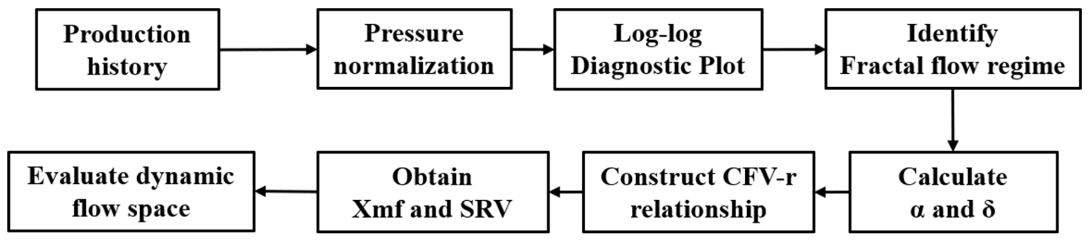
Based on the CFV concept introduced in Section 3.2, the CFV can be obtained from field production data via Equation (14), while the theoretical relationship between CFV and pressure propagation distance is given by Equation (15). By matching the two, the effective half-width of the fracture system ($X_{mf}$) and the skin factor ($S$) can be inverted (Figure 5).

3.3.1. Production Data and Preprocessing

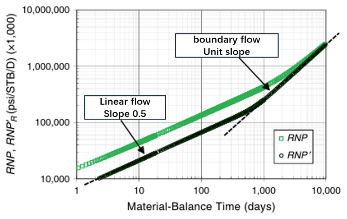
A pressure-derivative diagnostic plot is constructed in log–log coordinates ($t\cdot dp/dt$ vs. $t$) to identify the dominant flow regimes (Figure 6). RNP is the rate-normalized pressure, and material balance time is an equivalent time that could eliminate the effects of the varying rate. The linear flow regime is characterized by a derivative slope of 1/2, which is used to calibrate the geometric fractal characteristics of the fracture system. The fractal flow regime exhibits a power-law slope ($\alpha$) between 0 and 1/2, from which $\delta$ is calculated via Equation (13). The boundary-dominated flow regime is identified by a derivative slope of 1, indicating that the pressure front has reached the closed outer boundaries.

3.3.2. Parameter Calculation and Fitting

Through the preceding steps, the value of $\delta$ is obtained. Taking the logarithm of both sides of Equation (15) gives

$$lgCFV=\lg \left({\displaystyle \frac{4X_{mf}\varphi h}{2\delta }}\right)+2\delta \ast lgr.$$

(17)

A plot of $\mathrm{l}\mathrm{g}CFV$ versus $\lg r$ yields a straight line, the slope ($k$) and intercept ($b$) of which are obtained by linear regression. The slope ($k$) should theoretically equal $2\delta$, serving as a validation of the $\delta$ value. The intercept ($b$) is used to calculate $X_{mf}$:

$$X_{mf}={\displaystyle \frac{2\delta }{4\varphi h}}·{10}^b$$

(18)

Additionally, during the fractal flow regime, normalized pressure is defined as

$$P_{norm}={\displaystyle \frac{∆p}{q}}$$

(19)

Dividing both sides of Equation (11) by $t$ and integrating with respect to time yields

$$p={\displaystyle \frac{m}{1-\delta }}{t}^{1-\delta }+C,$$

(20)

where $C$ is the integration constant. Substituting Equation (18) into the above expression gives

$$P_{norm}={\displaystyle \frac{m}{1-\delta }}·t^{1-\delta }+S,$$

(21)

where $S$ is the fitting intercept, which is non-zero and reflects the additional pressure drop caused by the skin effect near the wellbore.

According to the earlier definition of $\delta =D_f/2$, substituting the distance ($r$) corresponding to the end of the first fractal segment (identified from flow-regime diagnosis) into Equation (15) yields the corresponding volume, which is taken as the stimulated reservoir volume:

$$SRV={\displaystyle \frac{4X_{mf}\varphi h}{2\delta }}{r}_{end}^{2\delta }$$

(22)

The resulting parameters are subsequently used to analyze the flow characteristics of fracture systems under different lithofacies conditions.

4. Discussion

4.1. Dynamic Flow Behavior of Gray Dolomite Reservoirs

As of April 2026, the four wells on Pad 2H (layered dolomite) have produced 1.89 × 10⁴ t over 525 days at 50 t/d, while the four wells on Pad 3H (laminated dolomite) have produced 0.41 × 10⁴ t over 192 days at 35 t/d. Both pads are located in the same sweet-spot area, enabling lithofacies comparison.

According to the fractal theory in Section 3, pressure propagation in complex fracture systems may deviate from integer-dimensional flow, exhibiting a power-law pressure-derivative response on log–log plots. The derivative slope (α) relates to the half-flow dimension ($\delta$) as follows: $\delta =1-\alpha$.

Here, $\delta$ describes the degree to which pressure propagation deviates from ideal linear flow. A value closer to 0.5 indicates behavior approaching classical linear flow, while lower values reflect more pronounced non-integer-dimensional diffusion characteristics.

Based on the rate-normalized pressure (RNP) and its derivative, flow regimes were identified for stages with stable pressure responses in the production history of the eight horizontal wells, and the corresponding $\alpha$ and $\delta$ values were calculated (

Table 3. Summary of flow-regime identification results.

Well Name	Lithofacies	$\mathit{\alpha }$	$\mathit{\delta }$
14-1	Layered dolomite	0.77029	0.22971
14-2	Layered dolomite	0.69254	0.30742
15-1	Layered dolomite	0.45321	0.54679
15-2	Layered dolomite	0.66745	0.33255
14-3	Laminated dolomite	0.75136	0.24864
14-4	Laminated dolomite	0.46650	0.5335
15-3	Laminated dolomite	0.70989	0.29011
15-4	Laminated dolomite	0.71602	0.28398

).

It should be noted that the flow-regime identification in this section is based on RNP vs. MBT diagnostic plots for qualitative assessment, aiming to detect the presence of power-law behavior and approximate slope ranges. This step serves to determine whether fractal flow exists rather than to obtain precise $\delta$ values. Subsequent FD-RTA parameter inversion employs square-root-of-time plots for quantitative matching. Although the $\delta$ values differ between the two approaches, the flow-regime classification (fractal vs. linear flow) remains consistent.

Among the eight wells, six exhibit α > 0.65, corresponding to δ mainly between 0.23 and 0.33, significantly deviating from the ideal linear flow value of 0.5. This indicates generally non-classical pressure propagation in the hydraulically fractured dolomite reservoir. Although the theoretical lower limit of $\delta$ in Acuna’s original model is 0.5 for linear flow, field-derived $\delta$ values below 0.5 are attributed to flow restriction caused by fracture closure, poor connectivity, or heterogeneous distribution that reduces the effective flow dimension, resulting in pressure propagation that deviates more significantly from the regular linear diffusion pattern. This behavior may be associated with complex fracture networks, multi-scale fracture connectivity, and locally dominant flow pathways.

A detailed breakdown of flow regimes and their durations for each well is presented in

Table 4. Flow regime and duration of linear flow of all wells.

Well Name	Lithofacies	Flow Regime	Duration of Linear Flow/d
14-1	Layered dolomite	Linear flow-boundary flow	19
14-2	Layered dolomite	Linear flow-transitional flow	37
15-1	Layered dolomite	Linear flow-transitional flow	58
15-2	Layered dolomite	Linear flow-boundary flow	21
14-3	Laminated dolomite	Linear flow-transitional flow	19
14-4	Laminated dolomite	Linear flow-transitional flow	68
15-3	Laminated dolomite	Linear flow-transitional flow	39
15-4	Laminated dolomite	Linear flow-transitional flow	27

. As shown, six of the eight wells are classified as “linear flow–transitional flow”, with the duration of the linear-flow segment ranging from 19 to 68 days. Notably, two wells, 2H15-1 and 3H14-4, exhibit relatively higher δ values (0.547 and 0.534, respectively), approaching a linear flow response, and both are classified as “linear flow–boundary flow”, suggesting that in certain areas, hydraulic fractures may form continuous dominant flow channels that enable pressure propagation closer to the regular fracture-controlled pattern. The longer linear-flow duration observed in these two wells (21 and 19 days, respectively) further supports the interpretation of sustained, connected fracture pathways, whereas the remaining wells show transitional behavior with shorter or moderate linear-flow durations.

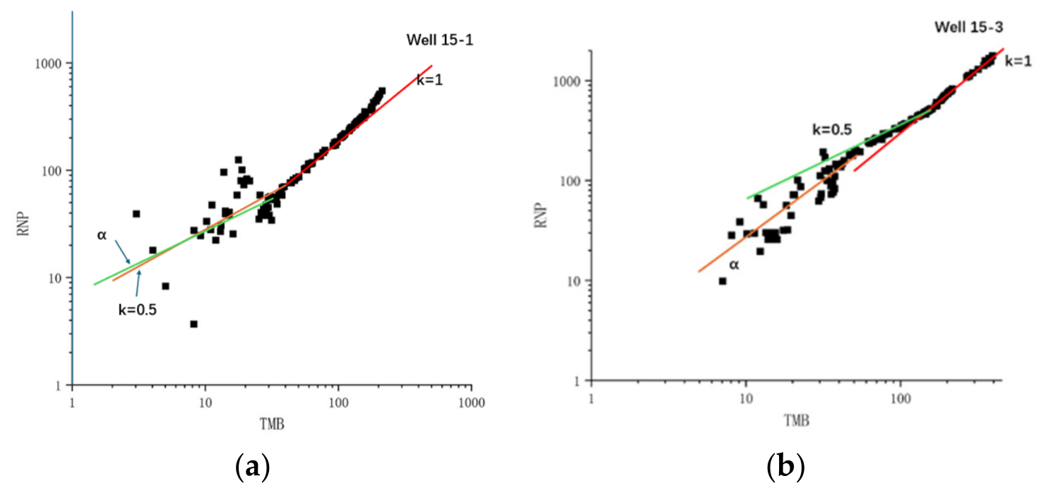
At the pad scale, δ ranges from 0.230 to 0.547 for Pad 2H and 0.249 to 0.534 for Pad 3H, with considerable overlap, indicating that the two lithofacies cannot be distinguished by flow dimension alone. Further integration with FD-RTA-derived effective fracture length and stimulated volume is required to evaluate the influence of lithofacies on effective flow-space development (Figure 7).

To illustrate the contrasting pressure propagation behaviors, Wells 2H15-1 and 3H15-3 are selected as representative cases. Well 2H15-1 exhibits α = 0.453 and $\delta$ = 0.547, with the pressure-derivative curve approaching the ideal linear-flow slope, indicating that pressure propagation is primarily controlled by relatively planar fracture channels. This response suggests that under layered dolomite conditions, locally continuous dominant fracture networks may develop. In contrast, Well 3H15-3 shows α = 0.710 and $\delta$ = 0.290, deviating significantly from linear flow and displaying a stronger fractal flow response. This indicates that pressure propagation in this well is influenced by multi-scale fracture systems with more complex spatial connectivity.

4.2. Fractal Parameter Estimation and Fracture-Network Characterization

Based on the FD-RTA workflow established in Section 3, history matching was performed on the production data of the eight horizontal wells. For each well, the production history was divided into consecutive stages according to major field events (wellbore cleanout, shut-in due to offset well fracturing, and subsequent production resumption); stage numbers (1, 2, and 3) denote the chronological sequence of these stages. Parameters including the half-flow dimension ($\delta$), fracture conductivity ($C_f$), effective fracture length ($X_f$), and dynamic effective stimulated volume ($A_{SRV}$) were obtained for each stage (Table 4).

As shown in

Table 5. Summary of FD-RTA inversion parameters.

Well Name	Stage	$\mathit{\delta }$	Fracture Conductivity/mD·m	Additional Pressure Drop/mD^ m2	OOIP/d	${\mathit{A}}_{\mathit{S}\mathit{R}\mathit{V}}$/1000 ∗ m3	Xf/ha	K/md
14-1	1	0.639	1431.71	70.74	26.69	9.6	32.9	1.26 × 10−3
14-1	2	0.325	68,601.36	294.77	43.60	15.6	53.8	6.50 × 10−2
14-1	3	0.699	162.75	931.35	9.74	3.5	12.0	4.23 × 10−4
14-2	1	0.501	6306.77	46.09	33.04	5.1	16.9	1.45 × 10−2
14-2	2	0.347	43,873.73	24.25	68.10	10.4	34.9	7.38 × 10−2
14-2	3	0.488	3665.29	1064.95	54.88	8.5	28.4	1.47 × 10−3
15-1	1	0.299	71,600.26	0	43.40	10.1	34.7	2.62 × 10−1
15-1	2	0.268	85,632.98	0	48.69	11.4	39.0	2.84 × 10−1
15-1	3	0.074	997,848.00	719.63	125.48	29.3	100.4	7.73 × 10−6
15-2	1	0.375	20,791.49	0	19.55	37.6	131.3	3.79 × 10−2
15-2	2	0.355	27,709.30	357.34	29.65	57.1	199.1	2.20 × 10−2
15-2	3	0.228	346,706.70	63.08	129.98	250.1	873.2	2.59 × 10−1
14-3	1	0.41	8610.60	1162.14	20.65	3.8	12.8	2.40 × 10−2
14-3	2	0.49	4514.16	682.52	56.47	66.7	226.6	1.51 × 10−3
14-4	1	0.422	7533.55	5.82	45.71	45.4	190.0	4.74 × 10−3
15-3	1	0.469	2989.84	128.36	17.24	14.2	49.0	9.56 × 10−3
15-3	2	0.678	340.75	0	78.82	65.0	224.1	1.72 × 10−4
15-4	1	0.507	2596.91	86.47	51.02	47.7	272.3	3.00 × 10−1

, $\delta$ values vary considerably across production stages for the eight wells, ranging from 0.074 to 0.699. This indicates that the effective pressure propagation mode is not fixed during production but is jointly influenced by fracture connectivity, conductivity, and reservoir heterogeneity. Notably, a decrease in $\delta$ may reflect two distinct physical scenarios: enhanced flow-path heterogeneity due to increased fracture-network complexity or flow contraction into fewer dominant pathways, reducing the effective flow dimension. Both scenarios result in $\delta$ deviating from 0.5, yet they imply different long-term productivity implications—the former may be accompanied by multi-scale fluid supply, whereas the latter suggests progressive drainage confinement to limited conduits.

Based on the temporal evolution of δ, the studied wells can be classified into three dynamic response patterns.

Pattern I: Continuous δ decline—dominant fracture control

Well 2H15-1 exhibits a typical decline trend, with δ decreasing from 0.299 to 0.268 to 0.074 across the three stages. During this period, $X_f$ increases from 34.7 ha to 100.4 ha, A_SRV increases from 10.1 × 10³ m³ to 29.3 × 10³ m³, and fracture conductivity rises from 7.16 × 10⁴ to 9.98 × 10⁵ mD·m. This combination—expanding drainage range and increasing conductivity alongside a declining flow dimension—indicates that production is sustained not by a complex network of uniformly distributed fractures but by a few high-conductivity dominant pathways. This behavior is consistent with the layered dolomite lithofacies, where relatively continuous bedding facilitates fracture propagation along preferential directions, forming well-connected dominant fracture systems.

Pattern II: Continuous δ increase—complex fracture-network expansion

Well 3H15-3 exhibits a clear increase in δ from 0.469 to 0.678, with A_SRV increasing from 14.2 × 10³ m³ to 65.0 × 10³ m³ and $X_f$ increasing from 49.0 ha to 224.1 ha. The simultaneous rise in δ and A_SRV suggests that the pressure propagation regime progressively expands from local dominant fractures to a multi-scale fracture system, activating additional storage space over time. Well 3H14-3 displays a similar pattern, with δ increasing from 0.410 to 0.490, A_SRV from 3.8 × 10³ m³ to 66.7 × 10³ m³, and $X_f$ from 12.8 ha to 226.6 ha. This behavior is attributed to the laminated dolomite lithofacies, where well-developed bedding planes act as mechanical weak surfaces during hydraulic fracturing, promoting fracture deflection, branching, and bedding-parallel opening, thereby forming multi-directional, multi-scale fracture networks.

Pattern III: Oscillatory δ—dynamic flow-space adjustment

A subset of wells exhibits oscillatory δ behavior. Well 2H14-1, for example, shows δ values of 0.639, 0.325, and 0.699 across its three stages. In Stage 2, $X_f$ increases to 53.8 ha, and A_SRV reaches 15.6 × 10³ m³, but both decline to 12.0 ha and 3.5 × 10³ m³, respectively, in Stage 3. This pattern indicates that the contribution of fractures at different scales varies over time, leading to dynamic reorganization and redistribution of effective flow space during production.

Overall, the FD-RTA results reveal that layered dolomite wells exhibit a wider range of $\delta$ variation (0.074–0.699) and generally higher fracture conductivity, reflecting a tendency toward dominant-fracture-controlled flow. In contrast, some laminated dolomite wells display simultaneous increases in $\delta$, $X_f$, and $A_{SRV}$, indicating progressive activation of multi-scale fractures over time. However, considerable overlap in the parameter ranges between the two lithofacies suggests that lithofacies control on dynamic flow behavior is statistical in nature rather than deterministic—local stress conditions, natural fracture development, and stimulation variations also influence individual well performance. More importantly, FD-RTA inversion provides dynamic information that microseismic evaluation alone cannot capture: the geometrically stimulated fracture volume does not fully translate into long-term effective flow space, and lithofacies structure, by controlling fracture propagation patterns and connectivity efficiency, governs the formation of dynamic effective flow space.

4.3. Relationship Between Fracture Complexity and Dynamic Flow Evolution

To investigate the relationship between fracture complexity and dynamic flow behavior, the microseismically derived b values are compared with the $\delta$ of Stage 1 obtained from FD-RTA inversion. The b-value characterizes fracture-size distribution complexity during fracturing, while the first-stage $\delta$ reflects the effective dimension of pressure propagation at initial production. Although both parameters relate to fracture-system architecture, they differ in origin—the b value is derived from microseismic magnitude distribution, and δ is derived from production performance—and their comparison helps reveal the link between geometric complexity and dynamic flow response.

Previous microseismic analysis indicates that layered and laminated dolomites exhibit similar dominant fracture dimensions but differ in fracture complexity. Laminated dolomite shows higher b-values, indicating a greater proportion of small-magnitude events, a more uniform fracture-size distribution, and more pronounced multi-scale fracture propagation.

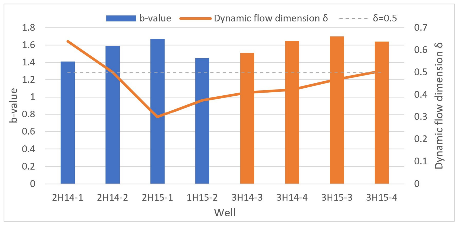
Figure 8 shows the b-values and Stage-1 $\delta$ for each well. Laminated dolomite wells exhibit higher b values than layered dolomite wells, consistent with their greater fracture complexity. The Stage-1 $\delta$ distribution also differs between the two lithofacies: laminated-dolomite $\delta$ ranges from 0.42 to 0.52 (average 0.47), while layered-dolomite δ ranges from 0.33 to 0.65 with a wider spread (average 0.46). Thus, laminated dolomite shows a more concentrated and slightly higher δ distribution, whereas layered dolomite contains both low-$\delta$ and high-$\delta$ end-members.

Notably, $\delta$ = 0.5 corresponds to ideal linear flow. Laminated dolomite wells have $\delta$ values close to 0.5, suggesting relatively regular fracture geometry in the early production stage. In contrast, Well 2H15-1 (layered) exhibits $\delta$ = 0.33, significantly deviating from linear flow, despite having a b value of 1.65, which is comparable to laminated dolomite levels. This implies that high fracture complexity (high b value) does not necessarily translate to a high flow dimension (high $\delta$) at initial production; factors beyond geometric complexity, such as fracture connectivity, conductivity, and effective stress, also govern $\delta$.

To further contrast the dynamic evolution of the two lithofacies, Wells 2H15-1 (layered, b = 1.65, and $\delta$ = 0.33) and 3H15-3 (laminated, b = 1.68, and $\delta$ = 0.50) are selected for comparison. These two wells are chosen because both exhibit high b values within their respective lithofacies, yet their Stage-1 $\delta$ values differ markedly—2H15-1 has a $\delta$ well below the laminated average, while 3H15-3 has a $\delta$ close to 0.5, at the high end of the laminated distribution. This contrast pair is most effective in addressing whether high fracture complexity necessarily translates into a high flow dimension.

FD-RTA multi-stage inversion shows that for 2H15-1, $\delta$ declines from 0.299 to 0.074, while $A_{SRV}$ increases from 10.1 × 10³ m³ to 29.3 × 10³ m³ and $X_f$ increases from 34.7 ha to 100.4 ha—indicating that the drainage range expands but the flow dimension continuously decreases, reflecting progressive contraction of flow into dominant fractures. For 3H15-3, $\delta$ increases from 0.469 to 0.678, $A_{SRV}$ increases from 14.2 × 10³ m³ to 65.0 × 10³ m³, and $X_f$ increases from 49.0 ha to 224.1 ha—indicating that both flow dimension and drainage range grow simultaneously, suggesting that more fracture scales become progressively activated over production.

In summary, b values and FD-RTA parameters characterize fracture-system effectiveness from complementary perspectives. The b values reflect the potential geometric complexity generated during fracturing, while FD-RTA parameters ($\delta$, $A_{SRV}$, and $X_f$) indicate the extent to which this potential is actually mobilized during production. A high b value does not guarantee a high δ or sustained $\delta$ growth; the actual effective flow space depends on fracture connectivity, conductivity, and dynamic evolution during production. In laminated dolomite, bedding planes promote multi-directional fracture propagation and multiscale connectivity, facilitating conversion of complex fracture networks into effective flow space. In layered dolomite, fractures tend to develop as oriented, less complex principal fracture systems, with production relying more on sustained supply from dominant pathways. Integrated assessment of hydraulic fracturing performance therefore requires both geometric complexity and dynamic flow response.

5. Conclusions

• Flow-regime identification based on RTA diagnostics shows that for most of the eight horizontal wells in the Yingxiongling dolomite reservoir, the initial half-flow dimension (δ₁) ranges from 0.299 to 0.639, significantly deviating from the ideal linear-flow value of 0.5. This indicates that post-fracturing pressure propagation is generally governed by multi-scale fracture networks, with pronounced fractal flow characteristics.
• Microseismic analysis indicates that layered and laminated dolomites exhibit similar dominant fracture dimensions but differ in fracture-network complexity. Laminated dolomite has higher b values than layered dolomite, reflecting the fact that laminated structures promote fracture deflection and branching during hydraulic fracturing, resulting in multi-scale fracture networks.
• FD-RTA inversion reveals distinct evolutionary patterns of dynamic effective flow space under different lithofacies conditions. Layered dolomite wells are predominantly characterized by dominant-fracture-controlled flow, with a sustained decline in δ and high fracture conductivity. Laminated dolomite wells are primarily characterized by complex-network-controlled flow, with δ and ASRV increasing simultaneously. A subset of wells exhibits oscillatory behavior, reflecting periodic reorganization of effective flow space.
• Cross-validation of microseismic b-values and FD-RTA parameters indicates that fracture geometric complexity does not simply correlate with dynamic effective flow. The b values reflect the potential geometric complexity generated during fracturing, while FD-RTA parameters reflect the extent to which this potential is actually mobilized during production—and the two are decoupled in some wells.
• Lithofabric controls the efficiency of converting geometric fracture space into dynamic effective flow space by governing fracture propagation patterns and connectivity. In laminated dolomite, bedding planes promote multi-directional fracture propagation, favoring the formation of progressively activated multi-scale connected networks. In layered dolomite, fractures tend to develop as oriented, low-complexity principal fracture systems, with production relying more on sustained supply from dominant pathways.

References

1. Oyekunle, A.A. Shale oil and gas revolution: Implications on energy market outlook and politics. In Proceedings of the SPE Nigeria Annual International Conference and Exhibition, Lagos, Nigeria, 5–7 August 2014. [Google Scholar] [CrossRef] [Scilit]
2. Temizel, C.; Canbaz, C.H.; Gok, I.M.; Roshankhah, S.; Palabiyik, Y.; Deniz-Paker, M.; Hosgor, F.B.; Ozyurtkan, H.; Aksahan, F.; Gormez, E.; et al. A thorough review and latest advances in shale reservoirs: Seismic to surveillance. In Proceedings of the SPE Latin American and Caribbean Petroleum Engineering Conference, Virtual, 27–31 July 2020. [Google Scholar]
3. Dou, L.R.; Wen, Z.X.; Wang, Z.M.; He, Z.J.; Song, C.P.; Chen, R.Y.; Liu, X.B.; Ji, T.Y.; Liu, Z.D.; Bian, H.G.; et al. Opportunities and challenges in global petroleum exploration. Oil Gas Geol. 2026, 47, 351–365. [Google Scholar]
4. Chen, Z.; Liu, H.L.; Li, Y.J.; Shen, Z.Q.; Xu, G.Q. Current status and development suggestions for shale oil reservoir stimulation at home and abroad. Pet. Drill. Tech. 2021, 49, 1–7. [Google Scholar] [CrossRef]
5. Hong, Z.; Meng, M.; Yuan, B.; Ma, C.; Wang, Q.; Deng, K.; Bao, J.; Yuan, M. Nanopore structure characterization of lacustrine and marine shales: Comparison between small angle neutron scattering and nitrogen adsorption methods. Int. J. Hydrogen Energy 2026, 208, 153565. [Google Scholar] [CrossRef] [Scilit]
6. Meng, M.; Li, Z.; Hong, Z.; Bao, J.; Jiang, Q. Quantifying pore size distribution by nuclear magnetic resonance method in tight sandstones: Comparison between water-wet and oil-wet saturated fluids. Int. J. Hydrogen Energy 2026, 197, 152608. [Google Scholar] [CrossRef] [Scilit]
7. Li, Q.W.; Ma, X.X.; Gao, B.; Chen, X.J. Progress and enlightenment of exploration and development of major shale oil zones in the USA. Xinjiang Pet. Geol. 2021, 42, 630–640. [Google Scholar]
8. Zhang, Y.J.; Wang, L.Y.; Liu, Y.F.; Zhang, J.L.; Zhou, D.S.; Ge, H.K. Advances and challenges of integration of fracturing and enhanced oil recovery in shale oil reservoirs. Pet. Drill. Tech. 2024, 52, 84–95. [Google Scholar] [CrossRef]
9. Zhou, Z.; Su, Y.; Wang, W.; Yan, Y. Integration of microseismic and well production data for fracture network calibration with an L-system and rate transient analysis. J. Unconv. Oil Gas Resour. 2016, 15, 113–121. [Google Scholar] [CrossRef] [Scilit]
10. Downie, R. Analysis of microseismic events associated with hydraulic fracture propagation. In Proceedings of the American Unconventional Resources Conference, Pittsburg, PA, USA, 5–7 June 2012. [Google Scholar]
11. Ilk, D.; Currie, S.M.; Symmons, D.; Rushing, J.A.; Broussard, N.J.; Blasingame, T.A. A comprehensive workflow for early analysis and interpretation of flowback data from wells in tight gas/shale reservoir systems. In Proceedings of the SPE Annual Technical Conference and Exhibition, Florence, Italy, 20–22 September 2010. [Google Scholar]
12. Clarkson, C.; Sun, H.; Cui, Y.; Cao, W.; Han, G.; Liu, W. Unconventional Reservoir Rate-Transient Analysis; Gulf Professional Publishing: Cambridge, MA, USA, 2022; ISBN 978-7-5183-55037. [Google Scholar]
13. Arps, J.J. Analysis of decline curves. Trans. AIME 1945, 160, 228–247. [Google Scholar] [CrossRef] [Scilit]
14. Fetkovich, M.J. Decline curve analysis using type curves. J. Pet. Technol. 1980, 32, 1065–1077. [Google Scholar] [CrossRef] [Scilit]
15. Clarkson, C.R.; Yuan, B.; Zhang, Z. A new straight-line analysis method for estimating fracture/reservoir properties using dynamic fluid-in-place calculations. SPE Reserv. Eval. Eng. 2020, 23, 606–626. [Google Scholar] [CrossRef] [Scilit]
16. Bao, J.; Meng, M.; Wang, Q.; Yu, S.; Yuan, M.; Hong, Z.; Jiang, Q. Comparison of square-root and logarithmic data treatment for pore connectivity by co-current spontaneous imbibition in lacustrine shales. Int. J. Hydrogen Energy 2026, 229, 154737. [Google Scholar] [CrossRef] [Scilit]
17. Rui, Z.; Zhang, F.; Liu, C.; Lu, R.; Emami-Meybodi, H.; Zhang, Z. A Two-Phase Rate Transient Analysis Method for Hydraulically Fractured Reservoirs with Different Fracture Geometries. SPE J. 2025, 30, 7037–7060. [Google Scholar] [CrossRef] [Scilit]
18. Chu, W.C.C.; Pandya, N.D.; Flumerfelt, R.W.; Chen, C. Rate-transient analysis based on the power-law behavior for permian wells. SPE Reserv. Eval. Eng. 2019, 22, 1360–1370. [Google Scholar] [CrossRef] [Scilit]
19. Mandelbrot, B.B. The fractal geometry of nature/b.b. Mandelbrot. Am. J. Phys. 1983, 51, 286. [Google Scholar] [CrossRef] [Scilit]
20. Miao, T.; Chen, A.; Xu, Y.; Cheng, S.; Yu, B. A fractal permeability model for porous–fracture media with the transfer of fluids from porous matrix to fracture. Fractals 2019, 27, 1950121. [Google Scholar] [CrossRef] [Scilit]
21. Liu, J.; Lu, M.; Sheng, G. Description of fracture network of hydraulic fracturing vertical wells in unconventional reservoirs. Front. Earth Sci. 2021, 9, 749181. [Google Scholar] [CrossRef] [Scilit]
22. Sun, H.; Li, Z.; Zhang, Y.; Chen, W. Fractional and fractal derivative models for transient anomalous diffusion: Model comparison. Chaos Solitons Fractals 2017, 102, 346–353. [Google Scholar] [CrossRef] [Scilit]
23. Berkowitz, B. Characterizing flow and transport in fractured geological media: A review. Adv. Water Resour. 2002, 25, 861–884. [Google Scholar] [CrossRef] [Scilit]
24. Wu, K.Y.; Liao, C.; Li, X.; Zhang, C.J.; Zhang, Q.; Li, G.M.; Zhang, J.; Tan, X.C. Geological characteristics of hydrocarbon pools in the Yingxiongling structural zone, Qaidam Basin. Geoscience 2020, 34, 378–389. [Google Scholar] [CrossRef]
25. Yao, Y.; Shen, Y.; Zhang, M.; Zhang, M. Identification and evaluation of fracturing advantageous lithofacies in the main structural zone of yingxiongling, qaidam basin. Processes 2025, 13, 3857. [Google Scholar] [CrossRef] [Scilit]
26. Acuña, J.A. Fractional dimension rate transient analysis applied to parent-child effects in unconventional wells. In Proceedings of the SPE/AAPG/SEG Unconventional Resources Technology Conference, Denver, CO, USA, 13–15 June 2023. [Google Scholar]
27. Acuña, J.A. Pressure and rate transient analysis in fracture networks in tight reservoirs using characteristic flow volume. In Proceedings of the SPE/AAPG/SEG Unconventional Resources Technology Conference, Austin, TX, USA, 24–26 July 2017. [Google Scholar]
28. O’Shaughnessy, B.; Procaccia, I. Diffusion on fractals. Phys. Rev. A 1985, 32, 3073–3083. [Google Scholar] [CrossRef] [Scilit] [PubMed]
Figure 1. Diagram of lithology ternary classification.
Fractalfract 10 00617 g001
Figure 2. Comparison of core photographs, thin-section images, and porosity between layered and laminated dolomite.
Fractalfract 10 00617 g002
Figure 3. Structural location map of the 2H and 3H platforms. (This vertical line is for locating the stratigraphic layer, showing the position of the positioning well).
Fractalfract 10 00617 g003
Figure 4. Top view of the microseismic events during fracturing. Left is platform 2 and right is platform 3 (Differenct colours means the different fracturing segments).
Fractalfract 10 00617 g004
Figure 5. Methodology workflow.
Fractalfract 10 00617 g005
Figure 6. Log–log plot of RNP and RNP’ versus MBT [12].
Fractalfract 10 00617 g006
Figure 7. Log–log diagnostic plots of RNP and RNP’ versus material balance time for representative wells. (a) Well 2H15-1 (layered dolomite, δ = 0.547, near-linear flow). (b) Well 3H15-3 (laminated dolomite, δ = 0.290, fractal flow).
Fractalfract 10 00617 g007
Figure 8. Comparison of microseismic b values and Stage-1 δ from FD-RTA inversion for the eight wells.
Fractalfract 10 00617 g008