Fractional-Order Composite Control Method for Beam Steering of Liquid Crystal Optical Phased Arrays

Abstract

To address the slow response, low pointing accuracy, and degraded stability caused by the coexistence of fractional-order dynamics, dual-axis coupling, and system delay in liquid crystal optical phased array (LCOPA) beam control, a fractional-order composite control method is proposed. First, the LCOPA is modeled as a two-input two-output system, and a fractional-order time-delay dynamic model is established. A composite control architecture integrating a fractional-order controller, a diagonal decoupling compensator, and a Smith predictor is then designed to improve dynamic response, suppress cross-axis coupling, and mitigate delay-induced performance degradation. A multi-strategy improved sparrow search algorithm is used to optimize the dual-channel fractional-order controller parameters, and closed-loop stability is verified using characteristic roots and the Matignon criterion. Simulation results show that the settling times of both axes are 11.50 ms, reduced by 62.54%/62.30%, 57.09%/56.11%, and 51.68%/48.89% compared with the results for PID, FOPID, and ADRC, respectively. The maximum cross-axis deviations are reduced to 0.0036° and 0.0030°, respsectively. Experiments further show that the mean absolute pointing errors of the X- and Y-axes decrease from 0.0466° and 0.0362° to 0.0057° and 0.0045°, while the RMSEs under external disturbances are 0.0060° and 0.0044°, respectively. These results demonstrate improved response speed, pointing accuracy, decoupling performance, and disturbance rejection.

1. Introduction

As a beam-steering device that realizes non-mechanical beam deflection through electrically controlled phase modulation, the liquid crystal optical phased array offers fast response, compact size, low power consumption, and ease of integration. It therefore has important application prospects in lidar, free-space optical communications, laser guidance, and other fields [1,2,3,4,5]. Compared with conventional mechanical scanning, an LCOPA can continuously control beam pointing through coordinated modulation of the phase distribution across array elements, enabling greater miniaturization and higher control accuracy [6,7,8]. However, because liquid-crystal materials exhibit viscoelasticity and hysteresis, practical operation is readily affected by time delay, disturbances, and channel coupling, which reduce beam-steering accuracy, slow the dynamic response, and impair system stability. High-performance controllers generally also contain many parameters to be optimized. Strong coupling among these parameters makes control performance sensitive to their configuration, making it difficult to satisfy requirements for speed, accuracy, and robustness simultaneously [9,10,11]. Therefore, research on high-performance control strategies and controller-parameter optimization for LCOPA beam-steering systems is of substantial theoretical and engineering value for achieving fast, accurate, and stable beam-pointing control.

Current research on LCOPA beam steering, both in China and internationally, focuses primarily on two areas: phase-distribution optimization, error compensation, and wavefront correction for improving beam-deflection accuracy; and closed-loop control strategies and control-parameter optimization for improving dynamic performance. For beam-deflection accuracy, existing studies primarily reduce the difference between actual and ideal deflection angles through phase-distribution design, drive-voltage correction, and wavefront-error compensation, thereby improving the open-loop pointing accuracy of LCOPAs. In 2010, Kong et al. [12] proposed a beam-steering method based on horizontal translation of phase steps. By iteratively adjusting the positions of the phase-step edges in a staircase phase wavefront, the method reduced the mean wavefront-slope error, significantly decreasing the deflection error caused by conventional quantized phase modulation and achieving high pointing accuracy at large deflection angles. In 2012, Zhou et al. [13] proposed a slope-approximation-based pointing-accuracy correction algorithm for liquid crystal phased arrays. The algorithm replaced the fitted wavefront slope with the approximate phase slope within a single electrode and iteratively adjusted the voltage-step height to reduce the deviation between the approximate and ideal slopes, thereby lowering pointing error and improving control accuracy. In 2013, Zhou et al. [14] proposed a pattern-search-based voltage-step correction algorithm that optimized the drive-voltage distribution to reduce the error between actual and ideal deflection angles, compensating beam-deflection error and significantly improving pointing accuracy. In 2016, Wang et al. [15] proposed a beam-steering method based on an improved periodic phase distribution. By optimizing the periodic phase profile, the method improved the linear correspondence between drive voltage and phase response, weakened the effect of the liquid-crystal device’s nonlinear response on beam deflection, and improved pointing accuracy during beam scanning, achieving a scanning pointing error below 5 rad. In 2021, Wang et al. [16] proposed a symmetric radial subaperture coherent-beam control method. Optimizing coherent control among subapertures reduced the effect of aperture variation on the deflection angle, suppressed scanning error, and improved pointing accuracy. In 2022, Fan et al. [17] proposed a particle-swarm-based pointing-accuracy optimization method. After analyzing the key factors affecting LCOPA pointing accuracy, the method used normalized accuracy error as the objective and searched for the optimal beam-control voltage to reduce deflection-angle error. In 2025, Ma [18] proposed a beam-deflection accuracy optimization method based on wavefront phase compensation. The actual phase surface was reconstructed through phase retrieval and wavefront compensation, and the phase grayscale distribution was corrected to suppress wavefront distortion and reduce beam-deflection error. For closed-loop control and parameter optimization, existing studies primarily improve the dynamic response, control accuracy, and disturbance rejection of LCOPA systems by introducing adaptive control, PID control, fractional-order control, and intelligent parameter tuning. In 2008, Orzechowski et al. [19] proposed an adaptive-control method based on nonlinear model compensation. It combined linear time-invariant feedback with adaptive control and incorporated a nonlinear model of the LCOPA beam-steering device into the adaptive controller to accurately characterize the nonlinear mapping from control commands to output deflection angles. This improved rejection of high-bandwidth, nonstationary disturbances and significantly enhanced robustness. In 2017, Xu et al. [20] proposed a PID tracking method for LCOPA-based free-space laser communications. Pixel displacement from the CCD center was used as the feedback variable, and PID closed-loop control generated beam-pointing-angle commands for rapid dynamic correction and stable tracking of the incident beam. In 2018, Wang et al. [21] proposed a fractional-order control method for LCOPA beam deflection. A closed-loop system with a CCD detector compared the desired and actual deflection angles and fed the error to a fractional-order controller to generate steering commands, enabling dynamic correction and improving deflection-angle accuracy. In 2021, Fan [22] proposed a BP-neural-network-based LCOPA beam-steering method. By combining the network’s online self-tuning capability with PID control, a closed-loop feedback system adaptively optimized the control parameters, reducing performance degradation caused by model uncertainty, external disturbances, and operating-condition changes while improving stability and disturbance rejection. In 2022, Wang et al. [23] proposed a system-identification-based three-step beam-deflection control method. Coordinated design of quasi-steady-state control, reference feedforward control, and error feedback control significantly improved response speed, tracking performance, and robustness, enabling fast, accurate, and stable beam deflection. In 2025, Tuo et al. [24] proposed a fractional-order PID beam-control method whose parameters were optimized using the phase-margin method. The tuning improved dynamic response and robustness, enabling fast, accurate, and stable LCOPA beam steering.

As shown in

Table 1. Comparison of representative beam-steering control methods for liquid crystal optical phased arrays.

Reference	Control Method	Main Advantage	Limitation	Main Focus
Orzechowski et al. [19]	Nonlinear adaptive control	Provides strong suppression capability for nonlinear and non-stationary disturbances	Relies on an adaptive model and does not simultaneously compensate for dual-axis coupling and time-delay effects	Nonlinearity/disturbance suppression
Xu et al. [20]	PID closed-loop control	Simple structure and easy implementation	Limited adaptability to complex dynamics and multivariable coupling	Beam-pointing tracking
Wang et al. [21]	Fractional-order control	Provides higher flexibility for regulating complex dynamic characteristics	Does not explicitly compensate for dual-axis coupling and time-delay effects	Dynamic response improvement
Fan et al. [22]	BP neural-network PID control	Enables online parameter adaptation	High implementation and training complexity; coupling and time-delay compensation are not explicitly considered	Parameter adaptation
Wang et al. [23]	Triple-step control	Improves response speed, tracking performance, and robustness through coordinated control	Multi-stage design; lacks dedicated compensation for fractional-order dynamics and dual-axis coupling	Dynamic performance enhancement
Ta et al. [24]	FOPID control with phase-margin tuning	Improves dynamic response performance and robustness	Mainly focuses on controller parameter tuning and does not simultaneously handle coupling and time-delay effects	Parameter optimization/dynamic performance
Proposed method	FOPID + diagonal decoupling compensation + Smith predictor	Simultaneously addresses fractional-order dynamics, dual-axis coupling, and time-delay effects through coordinated compensation	Higher structural and parameter design complexity	Coordinated control of fractional-order dynamics, coupling, and time delay

, LCOPA beam-steering research has gradually evolved from early phase-correction methods aimed at improving open-loop pointing accuracy to integrated control methods that combine closed-loop feedback and parameter optimization. Existing methods have achieved certain progress in improving static pointing accuracy, dynamic response speed, and disturbance rejection capability; however, several limitations still remain. Phase-distribution optimization and error-compensation methods mainly emphasize open-loop or quasi-static accuracy and provide limited improvement in dynamic control under liquid-crystal viscoelasticity, hysteresis, and time-varying disturbances. Existing closed-loop methods can improve stability and robustness, but their controllers have many strongly coupled parameters, and conventional empirical tuning or a single optimization strategy cannot easily balance speed, accuracy, and robustness. A composite-control and parameter-optimization method that combines enhanced dynamics with efficient parameter tuning is therefore needed to improve overall beam-steering performance under complex operating conditions.

Therefore, to address the issues of time delay, disturbances, and channel coupling in LCOPA beam-steering systems, this paper proposes a composite-control-based beam-steering method for LCOPA systems, aiming to overcome the limitations of conventional control methods in simultaneously achieving high beam-steering accuracy, fast dynamic response, and stable performance under complex operating conditions. The proposed method establishes a composite control strategy consisting of a fractional-order controller, a diagonal decoupling compensator, and a Smith predictor and incorporates a multi-strategy fusion sparrow search algorithm to optimize the controller parameters, thereby forming a coordinated control mechanism integrating fractional-order regulation, coupling compensation, time-delay prediction, and parameter optimization. Specifically, the fractional-order controller is employed to enhance the system adaptability to complex dynamic characteristics, the diagonal decoupling compensator is used to suppress the coupling effects between the two channels, the Smith predictor is introduced to mitigate the adverse effects of time delay on system stability and control performance, and the improved sparrow search algorithm is adopted to efficiently optimize the control parameters. Consequently, high-precision, fast, and robust beam-steering control of the LCOPA system is achieved. To quantitatively evaluate the effectiveness of the proposed method, the settling time, overshoot, and steady-state error are employed to assess the dynamic response performance and steady-state control accuracy of the system. The maximum coupling deviation and coupling degree are used to evaluate the dual-axis decoupling performance, while the beam-pointing error under external disturbances is adopted to assess the disturbance rejection capability. Meanwhile, the proposed method is compared with PID, FOPID, and ADRC under identical simulation conditions to quantitatively evaluate its performance improvements.

The remainder of this paper is organized as follows. Section 2 introduces the beam-steering principle of the LCOPA and establishes a two-input two-output fractional-order time-delay dynamic model. Section 3 presents a composite control strategy consisting of a fractional-order controller, a diagonal decoupling compensator, and a Smith predictor. Section 4 shows the employment a multi-strategy fusion sparrow search algorithm to optimize the control parameters. Section 5 analyzes the system stability based on the closed-loop characteristic roots and the Matignon criterion. Section 6 evaluates the control performance through comparative simulations involving PID, FOPID, ADRC, and the proposed method. Section 7 shows the establishment of an experimental platform and the completion of experiments on beam pointing, decoupling, and robustness. The conclusions of this paper are presented in the final section.

2. Beam-Steering Principle and Dynamic Modeling of the LCOPA

2.1. Beam-Steering Principle

The LCOPA beam-steering system is based on electrically controlled phase modulation. A grayscale image loaded by the silicon backplane circuit is converted into a spatial voltage distribution. The electric field formed between the transparent and control electrodes reorients the liquid-crystal molecules, changing their birefringence and producing a spatial phase-delay distribution corresponding to the input grayscale image.

As the incident beam passes through the liquid-crystal layer, the optical wave at each pixel experiences a spatially controllable phase delay. After reflection from the mirror, the modulated wave passes through the liquid-crystal layer again. Controlling this spatial distribution continuously adjusts the output-beam direction, thereby achieving non-mechanical two-dimensional beam deflection. The LCOPA beam-steering mechanism is illustrated in Figure 1.

$$\theta =\arcsin ({\displaystyle \frac{\lambda \Delta \varphi (v(m,n))}{2\pi d}})$$

(1)

where $\lambda$ is the wavelength of the incident light, $\Delta \varphi (v(m,n))$ denotes the phase difference between adjacent spatial pixels, $v(m,n)$ is the voltage matrix, $(m,n)$ is the number of LCOPA elements, and $d$ is the element pitch. This expression shows how phase differences generated by different control voltages under grayscale-image driving affect the output-beam deflection angle, thereby enabling dynamic control of the beam direction.

2.2. Dynamic Modeling of the Beam-Steering System

The LCOPA changes the effective refractive-index distribution of the liquid-crystal layer by applying drive voltages of different amplitudes to the pixel elements and controlling the molecular orientation within them. The resulting refractive-index variation further modulates the phase difference between adjacent elements, ultimately deflecting the output beam [25]. The LCOPA beam-steering process is therefore fundamentally a dynamic process driven by the input phase difference and characterized by the output deflection angle [26]. It can be represented as a two-input, two-output dynamic system:

$$\left[\begin{array}{c}{\theta }_x\\ {\theta }_y\end{array}\right]=\left[\begin{array}{cc}{G}_{11}(s)& G_{12}(s)\\ G_{21}(s)& G_{22}(s)\end{array}\right]\left[\begin{array}{c}\Delta {\phi }_x\\ \Delta {\phi }_y\end{array}\right]$$

(2)

where ${\theta }_x$ and ${\theta }_y$ are the output beam-deflection angles along the X and Y axes, respectively; $\Delta {\phi }_x$ and $\Delta {\phi }_y$ are the input phase differences applied in the X and Y directions, respectively; $G_{11}(s)$ and $G_{22}(s)$ are the main-channel transfer functions in the X and Y directions, respectively; and $G_{12}(s)$ and $G_{21}(s)$ are the two-axis coupling transfer functions. The parameters of the LCOPA beam-steering dynamic model are estimated using a Gegenbauer wavelet operational-matrix identification method for fractional-order time-delay systems. The X-channel output responses of the actual system and the identified model under an X-channel input are compared in Figure 2.

The main-channel transfer functions are

$$G_{11}(s)=G_{22}(s)={\displaystyle \frac{9.4775\times {10}^{-6}}{5.231\times {10}^{-4}{s}^{1.92}+1.661\times {10}^{-3}{s}^{1.20}+6.330\times {10}^{-4}{s}^{0.05}+2.82\times {10}^{-11}}}{e}^{-3.2s}$$

(3)

Similarly, the Y-channel output responses of the actual system and the identified model under a Y-channel input are compared in Figure 3.

The coupling-channel transfer functions are

$$G_{12}(s)={\displaystyle \frac{6.7231\times {10}^{-7}}{5.231\times {10}^{-4}{s}^{1.92}+1.661\times {10}^{-3}{s}^{1.20}+6.330\times {10}^{-4}{s}^{0.05}+2.82\times {10}^{-11}}}{e}^{-3.2s}$$

(4)

The Y-channel output responses of the actual system and the identified model under an X-channel input are compared in Figure 4.

$$G_{22}(s)={\displaystyle \frac{5.5601\times {10}^{-7}}{5.231\times {10}^{-4}{s}^{1.92}+1.661\times {10}^{-3}{s}^{1.20}+6.330\times {10}^{-4}{s}^{0.05}+2.82\times {10}^{-11}}}{e}^{-3.2s}$$

(5)

The X-channel output responses of the actual system and the identified model under a Y-channel input are compared in Figure 5.

The model describes the LCOPA beam-steering process using transfer functions in the Laplace domain, facilitating system analysis.

3. Composite Beam-Steering Control Strategy

The LCOPA beam-steering system simultaneously exhibits fractional-order dynamic characteristics, dual-axis channel coupling, and system time delay, making it difficult for a single control structure to provide targeted compensation for all of these characteristics. In terms of control scheme selection, conventional PID or standalone fractional-order PID controllers have relatively simple structures, but they mainly improve system dynamics through error-feedback regulation and cannot explicitly compensate for dual-axis coupling and time delay at the same time. Active disturbance rejection control can enhance disturbance rejection through state observation and disturbance compensation; however, for a two-input two-output system with both coupling and time delay, additional designing of multichannel observers and associated parameters is required. Model predictive control can handle multivariable coupling and constraints within a unified framework, but it generally requires online receding-horizon optimization during the control process, placing relatively high demands on model accuracy and real-time computational capability.

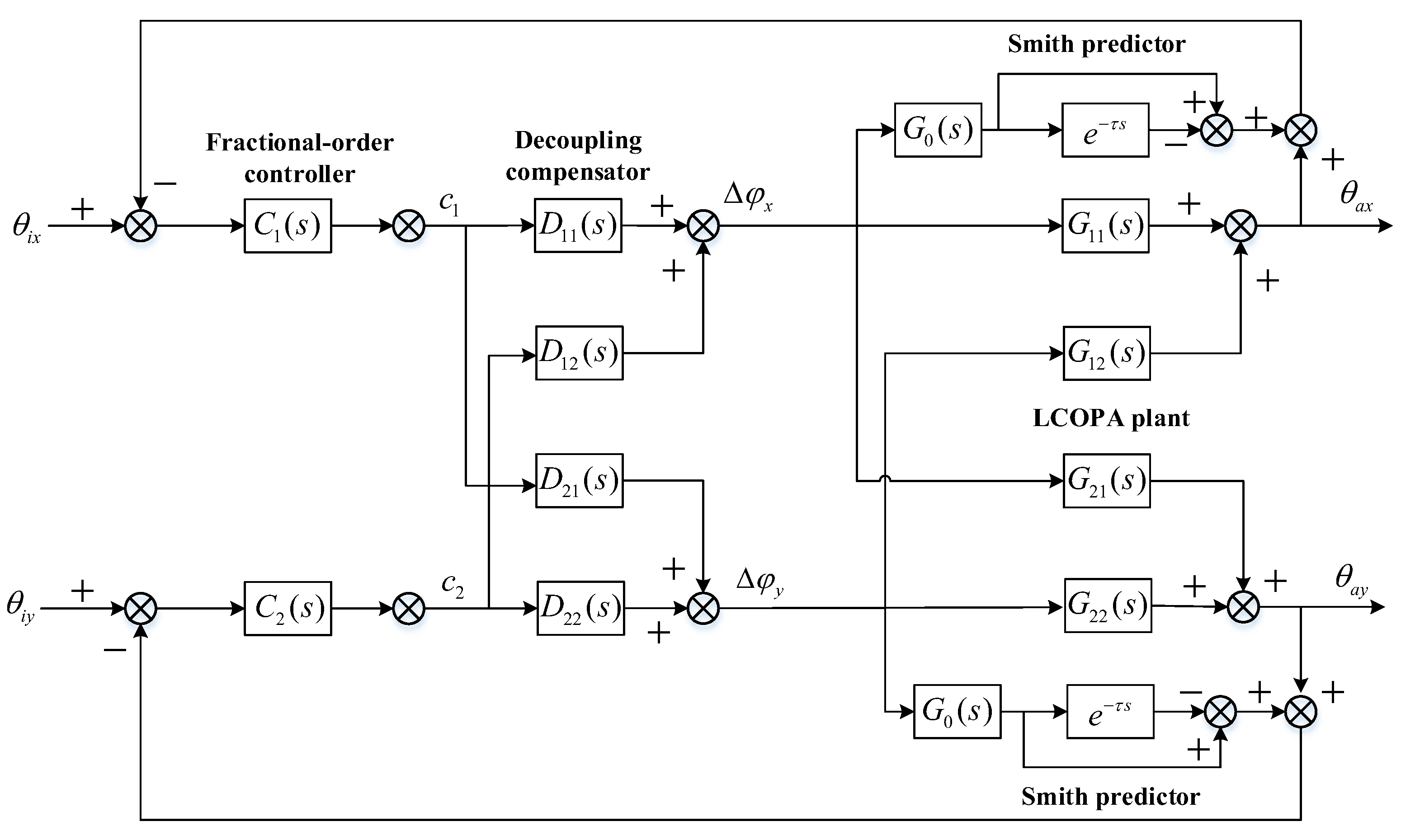
Considering that the LCOPA dynamic model established in this study can separately characterize fractional-order dynamics, dual-axis coupling, and time-delay effects, a modular compensation strategy corresponding to these characteristics is adopted. Accordingly, a composite control strategy consisting of a fractional-order controller, a diagonal decoupling compensator, and a Smith predictor is constructed, as shown in Figure 6.

The proposed strategy achieves targeted regulation of different dynamic characteristics through the coordinated mechanism of “fractional-order regulation–coupling compensation–time-delay prediction.” Specifically, the fractional-order controller introduces fractional-order integral and differential operators to provide additional tuning degrees of freedom, thereby enabling better adaptation to the fractional-order dynamic characteristics of the LCOPA system [27]. The diagonal decoupling compensator is constructed according to the two-input two-output plant model and introduces compensation channels to attenuate the cross-coupling terms in a feedforward manner, thereby reducing the mutual influence between the two axes [28]. The Smith predictor constructs a predictive channel using the plant model and its time-delay model to mitigate the adverse effects of pure time delay on the feedback regulation process and closed-loop dynamic performance [29]. The structural parameters of the diagonal decoupling compensator and the Smith predictor are directly determined from the identified plant model, whereas the parameters of the fractional-order controller are optimized offline using the subsequent multi-strategy fusion sparrow search algorithm. Therefore, the parameter optimization process is not involved in the real-time control loop, which reduces the additional real-time computational burden introduced by the intelligent optimization algorithm.

Specifically, the fractional-order controllers $C_1(s)$ and $C_2(s)$ act on the X- and Y-axis control channels, respectively, and regulate the main-channel dynamics through fractional-order integral and differential operators. Compared with integer-order PID control, the additional fractional orders of integration and differentiation provide extra degrees of freedom for shaping the system dynamics, enabling more flexible trade-offs among response speed, steady-state accuracy, and robustness. Considering the cross-coupling effect in the beam-steering process, where an input applied to one channel may induce an additional deflection in the other channel, diagonal decoupling compensators $D_{11}(s)$, $D_{12}(s), D_{21}(s)$ and $D_{22}(s)$ are further introduced at the controller output. By constructing compensation channels based on the plant model, the cross-coupling terms are compensated in a feedforward manner so that the two-input two-output system can be approximately decomposed into two relatively independent control loops, thereby reducing the adverse effect of channel coupling on beam-pointing accuracy.

In addition, to mitigate the phase lag and degradation of closed-loop performance caused by pure time delay, a Smith predictor is further incorporated into the decoupled control structure. The predictor constructs a predictive compensation channel based on the plant model $G_0(s)$ and its time-delay term $e^{-\tau s}$. By estimating the delay-free response of the system, the adverse influence caused by the direct inclusion of the time delay in the main feedback loop can be reduced, thereby improving the dynamic response performance of the system. It should be noted that the compensation performance of the Smith predictor depends on the matching accuracy of the plant model and the time-delay parameters. When relatively large model uncertainties exist, its compensation effectiveness may deteriorate. Therefore, the robustness of the proposed method is further evaluated in this study through parameter-variation simulations and physical disturbance experiments.

In summary, the proposed composite control architecture is not a simple superposition of different control components but rather a targeted and coordinated design developed according to the fractional-order dynamics, dual-axis coupling, and time-delay characteristics of the LCOPA beam-steering system. While retaining a modular implementation, the proposed architecture provides dedicated compensation for the main-channel dynamics, cross-channel coupling, and time-delay effects, while avoiding the need for online receding-horizon optimization during real-time control. The closed-loop stability of the decoupled dual-channel system is further verified based on the closed-loop characteristic roots and the Matignon stability criterion, and its overall control performance is evaluated through comparative simulations with PID, FOPID, and ADRC methods.

3.1. Fractional-Order Controller Design

A conventional integer-order PID controller contains only proportional, integral, and derivative parameters and cannot fully characterize the complex dynamics of the LCOPA beam-deflection system. To increase the controller’s freedom to shape the dynamics, fractional integral and derivative orders are introduced into the integer-order PID structure to form a fractional-order $P{I}^{\lambda }{D}^{\mu }$ controller. Compared with a conventional PID controller, the additional adjustable integral order $\lambda$ and derivative order $\mu$ enable more flexible construction of frequency-domain characteristics and time-domain responses, improving accuracy and robustness.

In the composite control architecture, fractional-order controllers $C_1(s)$ and $C_2(s)$ act on control channels $x$ and $y$, respectively, and are expressed as

$$C_1(s)={\displaystyle \frac{Y_1(s)}{E_1(s)}}=K_{p_1}+{\displaystyle \frac{K_{i_1}}{s^{{\lambda }_1}}}+K_{d_1}{s}^{{\mu }_1}(0<{\lambda }_1,{\mu }_1<2)$$

(6)

$$C_2(s)={\displaystyle \frac{Y_2(s)}{E_2(s)}}=K_{p_2}+{\displaystyle \frac{K_{i_2}}{s^{{\lambda }_2}}}+K_{d_2}{s}^{{\mu }_2}(0<{\lambda }_2,{\mu }_2<2)$$

(7)

where $E_1(s)$ and $E_2(s)$ are the error signals in channels $x$ and $y$, respectively; $Y_1(s)$ and $Y_2(s)$ are the controller outputs; $K_{p_1}, K_{i_1}, K_{d_1}$ and $K_{p_2}, K_{i_2}, K_{d_2}$ denote the proportional, integral, and derivative gains of the two channel controllers, respectively; ${\lambda }_1, {\lambda }_2$ is the fractional integral order; and ${\mu }_1, {\mu }_2$ is the fractional derivative order. When ${\lambda }_1={\mu }_1=1$ or ${\lambda }_2={\mu }_2=1$, the fractional-order controller reduces to a conventional integer-order PID controller.

Mechanistically, the fractional integral term provides more flexible accumulation at low frequencies, helping reduce steady-state error and improve rejection of slowly varying disturbances. The fractional derivative term accelerates the dynamic response while reducing the excessive amplification of high-frequency noise associated with a conventional integer-order derivative, thereby improving closed-loop damping and stability margins. Proper selection of $\lambda$ and $\mu$ provides greater flexibility in balancing response speed, overshoot, steady-state accuracy, and robustness.

For the LCOPA beam-deflection system, the fractional-order controller better accommodates the non-integer-order dynamics of the liquid crystal device, improves adaptability to complex operating conditions and external disturbances, and provides a stable inner control loop for subsequent coupling and time-delay compensation. It is therefore the core regulating element of the proposed composite strategy.

3.2. Diagonal Decoupling Compensator Design

The LCOPA beam-deflection plant is generally a two-input, two-output system, and the deflection directions $x$ and $y$ are not completely independent. In practice, a step change in one channel affects not only that channel’s output but may also disturb the other channel through internal element coupling, causing output deviation, increased steady-state error, and reduced control accuracy. When coupling is strong, treating the two directions as independent single-input, single-output systems cannot provide satisfactory closed-loop performance.

To weaken inter-channel coupling, a diagonal decoupling compensator is introduced at the output of the fractional-order controller. Compensation channels are constructed from the plant model to correct the coupling terms by feedforward action, making the original coupled system approximate two relatively independent control loops. For the composite architecture shown in Figure 6, the derivation is as follows.

Let the system inputs be the two-channel phase increments $\Delta {\phi }_x$ and $\Delta {\phi }_y$, and the outputs be the corresponding deflection angles ${\theta }_{ax}$ and ${\theta }_{ay}$. The input–output transfer relationship is

$$\left[\begin{array}{c}{\theta }_{ax}\\ {\theta }_{ay}\end{array}\right]=\left[\begin{array}{cc}{G}_{11}(s)& G_{12}(s)\\ G_{21}(s)& G_{22}(s)\end{array}\right]\left[\begin{array}{c}\Delta {\phi }_x\\ \Delta {\phi }_y\end{array}\right]$$

(8)

A decoupling compensator $c_1$ is inserted between controller outputs $c_2$, $D(s)$ and the system inputs, giving

$$\left[\begin{array}{c}\Delta {\phi }_x\\ \Delta {\phi }_y\end{array}\right]=\left[\begin{array}{cc}{D}_{11}(s)& D_{12}(s)\\ D_{21}(s)& D_{22}(s)\end{array}\right]\left[\begin{array}{c}{c}_1\\ c_2\end{array}\right]$$

(9)

The compensated system output can then be written as

$$\left[\begin{array}{c}{\theta }_{ax}\\ {\theta }_{ay}\end{array}\right]=\left[\begin{array}{cc}{G}_{11}(s)& G_{12}(s)\\ G_{21}(s)& G_{22}(s)\end{array}\right]\left[\begin{array}{cc}{D}_{11}(s)& D_{12}(s)\\ D_{21}(s)& D_{22}(s)\end{array}\right]\left[\begin{array}{c}{c}_1\\ c_2\end{array}\right]=G(s)D(s)\left[\begin{array}{c}{c}_1\\ c_2\end{array}\right]$$

(10)

In theory, setting $G(s)D(s)=I$ achieves complete system decoupling, i.e., $D(s)=G^{-1}(s)$. However, this method also changes the intrinsic dynamics of the main channels and is sensitive to plant-model accuracy, making it vulnerable to parameter perturbations and noise in engineering applications. The present work instead focuses on attenuating the coupling terms while preserving the main-channel dynamics as much as possible. A diagonal decoupling design is therefore adopted, such that the compensated system satisfies

$$\left[\begin{array}{cc}{G}_{11}(s)& G_{12}(s)\\ G_{21}(s)& G_{22}(s)\end{array}\right]\left[\begin{array}{cc}{D}_{11}(s)& D_{12}(s)\\ D_{21}(s)& D_{22}(s)\end{array}\right]=\left[\begin{array}{cc}{G}_{11}(s)& 0\\ 0& G_{22}(s)\end{array}\right]$$

(11)

The decoupling compensator matrix is thus

$$D(s)=G^{-1}(s)\left[\begin{array}{cc}{G}_{11}(s)& 0\\ 0& G_{22}(s)\end{array}\right]$$

(12)

Expanding the decoupling compensator matrix gives

$$D(s)={\displaystyle \frac{1}{G_{11}(s)G_{22}(s)-G_{12}(s)G_{21}(s)}}\left[\begin{array}{cc}{G}_{11}(s)G_{22}(s)& -G_{12}(s)G_{22}(s)\\ -G_{11}(s)G_{21}(s)& G_{11}(s)G_{22}(s)\end{array}\right]$$

(13)

The decoupling compensator matrix can be written as

$$D(s)={\displaystyle \frac{G_{11}(s)G_{22}(s)}{G_{11}(s)G_{22}(s)-G_{12}(s)G_{21}(s)}}\left[\begin{array}{cc}1& -{\displaystyle \frac{G_{12}(s)}{G_{11}(s)}}\\ -{\displaystyle \frac{G_{21}(s)}{G_{22}(s)}}& 1\end{array}\right]$$

(14)

Using the identified system parameters, the diagonal decoupling compensator is approximated by

$$D(s)=\left[\begin{array}{cc}1.0041& -0.0582\\ -0.0703& 1.0041\end{array}\right]$$

(15)

As Expression (15) shows, the compensator retains unit gain on the main diagonal and corrects cross-coupling through feedforward diagonal compensation terms. Specifically, $D_{12}(s)$ compensates the coupling from channel $y$ to channel $x$, while $D_{21}(s)$ compensates the coupling from channel $x$ to channel $y$.

In summary, introducing the diagonal decoupling compensator at the controller output effectively weakens inter-channel coupling while preserving the main-channel dynamics. The two-input, two-output system is approximately decomposed into two independent single-channel loops, improving beam-steering accuracy and providing a basis for Smith predictor design and enhanced closed-loop performance.

3.3. Smith Predictor Compensator Design

In addition to non-integer-order dynamics and channel coupling, the LCOPA beam-deflection system commonly contains pure time delay arising from liquid crystal response inertia, drive-circuit processing, and control-signal transmission. Pure delay introduces additional phase lag, reduces the phase margin, limits closed-loop bandwidth, and slows the system response. Poor parameter design may also cause oscillation or even instability. Conventional feedback alone therefore often cannot satisfy both response-speed and stability requirements.

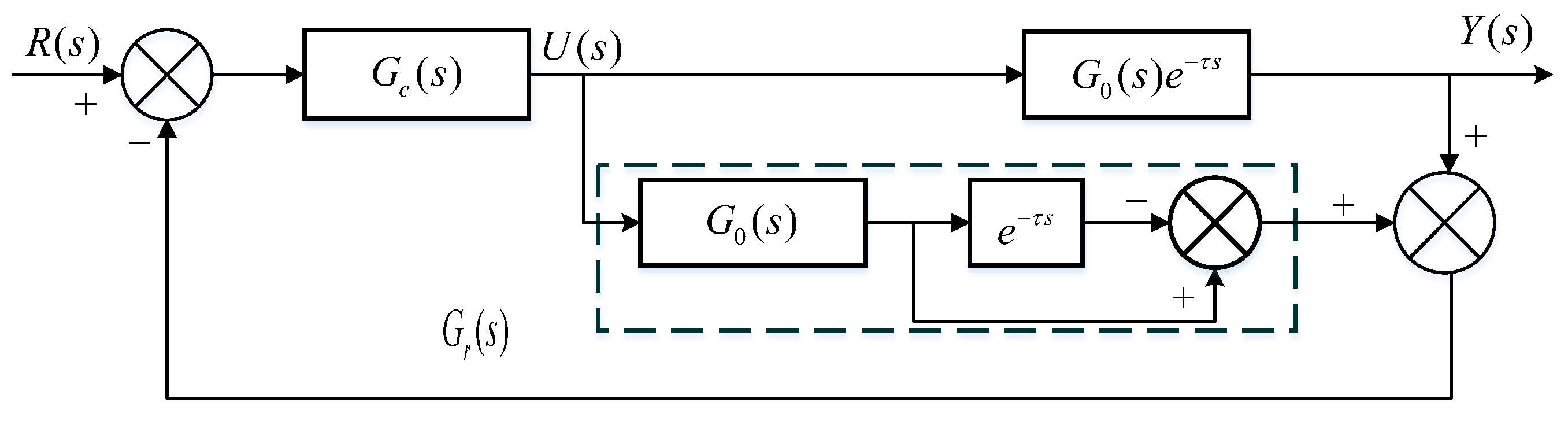
To mitigate the adverse effect of pure delay on closed-loop performance, a Smith predictor compensator is introduced after diagonal decoupling. Smith predictor control decomposes a time-delay plant into a delay-free part and a pure-delay part and constructs an internal plant model whose output estimates the delay-free response. Controller design and regulation can then focus primarily on the delay-free plant, preventing the delay from entering the main feedback loop directly. The principle of the Smith predictor compensator is shown in Figure 7.

After compensator $G_r(s)$ is introduced, the transfer function of the equivalent plant is

$${\displaystyle \frac{Y(s)}{R(s)}}=G_0(s)e^{-\tau s}+G_r(s)$$

(16)

where $G_0(s)$ is the delay-free plant model, and $\tau$ is the system delay. In the Smith predictor structure, a predictive model $G_0(s)$ and delay element $e^{-\tau s}$ corresponding to the plant are constructed within the control system, and compensator $G_r(s)$ is expressed as

$$G_r(s)=G_0(s)(1-e^{-\tau s})$$

(17)

The compensated closed-loop transfer function is

$$\varphi (s)={\displaystyle \frac{G_c(s)G_0(s)e^{-\tau s}}{1+G_c(s)[G_0(s)e^{-\tau s}+G_0(s)(1-)e^{-\tau s}]}}={\displaystyle \frac{G_c(s)G_0(s)}{1+G_c(s)G_0(s)}}{e}^{-\tau s}$$

(18)

The system characteristic T is therefore

$$1+G_c(s)G_0(s)=0$$

(19)

As can be seen from Equation (19), under the ideal condition that the plant model and its time-delay parameters accurately match the actual system, the pure time-delay term no longer explicitly appears in the nominal closed-loop characteristic equation. Therefore, the controller can be designed primarily for the delay-free plant, thereby mitigating the adverse effects of time delay on closed-loop stability and dynamic performance. It should be noted that Smith predictor compensation cannot eliminate the physical time delay inherent in the actual system, and its effectiveness depends on the accuracy of the plant model and the associated time-delay parameters. When model parameter deviations, unmodeled dynamics, or time-delay variations are present, discrepancies may arise between the predicted output and the actual output, leading to degraded delay-compensation performance and potentially affecting system robustness and closed-loop performance. Therefore, the Smith predictor employed in this study is intended to mitigate, rather than completely eliminate, the influence of time delay.

4. Control-Parameter Optimization Based on a Multi-Strategy Fusion Sparrow Search Algorithm

As indicated by the composite strategy above, the Smith predictor and diagonal decoupling compensators are designed mainly from the system model; their structural parameters can be determined from the plant model and are not the primary optimization variables here. By contrast, the fractional-order $P{I}^{\lambda }{D}^{\mu }$ controller contains multiple parameters to be tuned, including $K_p, K_i, K_d, \lambda , \mu$. These parameters are strongly coupled and directly affect response speed, steady-state error, and robustness. To achieve high-accuracy, as well as fast and robust LCOPA beam steering, this paper therefore uses a multi-strategy fusion sparrow search algorithm to tune the controller parameters, with ITAE as the performance index, enabling efficient optimization of the composite controller.

4.1. Design of the Multi-Strategy Fusion Sparrow Search Algorithm

The sparrow search algorithm (SSA) is a swarm-intelligence optimizer that simulates sparrow foraging and antipredation behavior. Coordinated searching by producers, scroungers, and sentinels enables the population to approach the optimum. SSA has a simple structure, few parameters, and straightforward implementation, but for complex high-dimensional optimization, it may have insufficient global-search capability, declining population diversity late in the iterations, and susceptibility to local optima.

Because composite-controller optimization has high parameter dimensionality, strong objective-function nonlinearity, and a complex search space, this paper augments standard SSA with a fitness-weighting mechanism, a multi-individual weighted-learning mechanism, and a Levy-flight perturbation mechanism. These mechanisms improve the position updates of producers, scroungers, and sentinels, respectively, yielding a multi-strategy fusion SSA with faster convergence, stronger global search, and more stable solutions.

(1) Population initialization and fitness representation.

Let the sparrow population size be $n$ and the optimization-problem dimension be $d$. The population position matrix is

$$X=\left[\begin{array}{cccc}{x}_{1,1}& x_{1,2}& \cdots & x_{1,d}\\ x_{2,1}& x_{2,2}& \cdots & x_{2,d}\\ ⋮& ⋮& & ⋮\\ x_{n,1}& x_{1,1}& \cdots & x_{n,d}\end{array}\right]$$

(20)

where $x_{i,j}$ is the position of sparrow $i$ in dimension $j$, with $i=1,2,3,\dots ,n$ and $j=1,2,\dots ,d$. The fitness values of the individuals in the population are

$$F=\left[\begin{array}{cccc}f(x_{1,1}& x_{1,2}& \cdots & x_{1,d})\\ f(x_{2,1}& x_{2,2}& \cdots & x_{2,d})\\ ⋮& ⋮& & ⋮\\ f(x_{n,1}& x_{1,1}& \cdots & x_{n,d})\end{array}\right]$$

(21)

where $f(\cdot )$ is the fitness function. In this study, the fitness function is determined by the controller-parameter tuning objective.

(2) Fitness-weighted producer update strategy.

Producers are the primary guides of the population’s search direction, so their search quality directly affects convergence speed and optimization accuracy. In standard SSA, producer positions are updated mainly through exponential decay and random perturbations. Although this provides some search capability, it underuses guidance from high-quality individuals. A fitness-weighting mechanism is therefore introduced into the producer update so that individuals with better fitness exert stronger directional guidance, improving convergence speed and optimization accuracy. The improved producer update is

$$X_{i,j}^{t+1}=\left\{\begin{array}{cc}{X}_{i,j}^t+(\gamma X_{best,j}^t-X_{i,j}^t)\cdot w_i,& R_2<S\\ X_{i,j}^t+QL,& R_2\ge S\end{array}\right.$$

(22)

where $t$ is the current iteration number, $X_{i,j}^t$ is the position of individual $i$ in dimension $j$, $\gamma \in (0,1)$ is a random weight, and $w_i$ is the normalized fitness weight of producer $i$. $R_2$ is the alarm value, $S$ is the safety threshold, $Q$ is a normally distributed random variable, and $L$ is an $1\times d$ matrix of ones.

When $R_2<S$, the current environment is considered safe. Guided by the current best position, producers search while their movement amplitudes are adjusted by the fitness weights. Producers with better fitness provide stronger directional guidance, helping the population converge rapidly toward high-quality regions.

When $R_2\ge S$, the population has detected danger. Random perturbations then move producers out of the current region, preventing premature aggregation near a local optimum. The sparrow population migrates to other regions and continues searching. This strategy strengthens the guidance of high-quality producers, accelerates movement toward promising regions, improves convergence speed and accuracy, and helps prevent premature convergence.

The normalized fitness weight $w_i$ is

$$w_i={\displaystyle \frac{f_{worst}-f_i+\epsilon }{{\displaystyle {\sum }_{k=1}^{N_p}(f_{worst}-f_i)+\epsilon }}}$$

(23)

where $N_p$ is the number of producers, $f_i$ is the fitness value of producer $i$, and $f_{worst}$ is the worst fitness in the current population.

(3) Multi-individual weighted-learning scrounger update strategy.

Scroungers usually constitute most of the population, and their search behavior strongly affects population diversity and global exploration. In standard SSA, some scroungers update mainly with reference to producer positions, which can produce a single search direction and reduce diversity. To strengthen scrounger learning, a multi-individual weighted-learning mechanism is introduced. Positional information from multiple reference individuals is fused to generate new search positions, increasing directional diversity and global exploration. The improved scrounger update is

$$X_{i,j}^{t+1}=\left\{\begin{array}{cc}Q\exp ({\displaystyle \frac{X_{\mathrm{worst}}^t-X_{i,j}^t}{\alpha i}}),& i>n/2\\ {\displaystyle \frac{P_a{x}_{a,j}+P_b{x}_{b,j}+P_c{x}_{a,j}}{P_a+P_b+P_c}},& i\le n/2\end{array}\right.$$

(24)

where $\alpha$ is an adjustment factor; $X_{worst,j}^t$ is the position of the current global worst individual in dimension $j$; $x_{a,j}$, $x_{b,j}$, and $x_{c,j}$ are the positions of three reference individuals in dimension $j$; and $P_a$, $P_b$, and $P_c$ are the corresponding weights. By combining multiple reference individuals, the strategy prevents scroungers from learning only from a single best individual, increasing directional diversity and global-search capability. Poor-fitness scroungers also use an exponential update that moves them away from the worst position and expands the search range, improving the ability to escape local optima.

$$\begin{array}{l}{P}_a={\displaystyle \frac{f_{worst}-f_a+\epsilon }{(f_{worst}-f_a)+(f_{worst}-f_b)+(f_{worst}-f_c)+3\epsilon }}\\ P_b={\displaystyle \frac{f_{worst}-f_b+\epsilon }{(f_{worst}-f_a)+(f_{worst}-f_b)+(f_{worst}-f_c)+3\epsilon }}\\ P_c={\displaystyle \frac{f_{worst}-f_c+\epsilon }{(f_{worst}-f_a)+(f_{worst}-f_b)+(f_{worst}-f_c)+3\epsilon }}\end{array}$$

(25)

When $i>n/2$, the scrounger ranks poorly in the population, and the current search region is of low quality. The individual must therefore expand its search range and move away from the poor region to strengthen global exploration.

When $i\le n/2$, the scrounger is relatively good. Rather than simply following the best producer, it selects multiple reference individuals and generates a new position through weighted learning. This prevents excessive concentration in a single direction and increases search diversity.

(4) Levy-flight-perturbed sentinel update strategy.

Sentinels detect external risk and guide the population out of dangerous regions; their update mechanism is closely related to robustness and the ability to escape local optima. Although standard SSA changes sentinel positions through random perturbations, the perturbation range is limited. Especially late in the iterations, the population can cluster in a local region and lose the ability to escape a local optimum. This study introduces Levy-flight perturbations into the sentinel update. The long-tailed Levy distribution allows both local search near the best position and occasional long-distance jumps, improving escape from local optima. The improved sentinel update is

$$X_{i,j}^{t+1}=\left\{\begin{array}{cc}Levy(d)\cdot X_{best}^t+B\left|X_{i,j}^t-Levy(d)\cdot X_{best}^t\right|,& f_i\ne f_b\\ X_{i,j}^t+k\cdot ({\displaystyle \frac{X_{i,j}^t-X_{worst,j}^t}{\left|f_i-f_w\right|+e}}),& f_i=f_b\end{array}\right.$$

(26)

where $Levy(d)$ is a random perturbation following the $Levy$ distribution; $X_{best}^t$ is the current global best position; $B$ is the controlled step length, with $B\sim N(0,1)$; $k\in [-1,1]$ is a random number; $f_i$ is the current individual’s fitness; $f_b$ and $f_w$ are the best and worst fitness values in the current population; and $e$ is a small positive constant that prevents division by zero.

When $f_i\ne f_b$, the individual is not the current best. A Levy-flight perturbation is introduced near the global best position, allowing large-step jumps that expand the search range and improve escape from local optima.

When $f_i=f_b$, the individual is near the current best position. Random perturbation moves it away from the worst-individual direction, preventing confinement to a local-optimum region while retaining local-search capability.

To clearly illustrate the coordinated execution of the three improvement strategies described above, the pseudocode of the multi-strategy fusion sparrow search algorithm is presented in Algorithm 1.

Algorithm 1 Multi-strategy fusion sparrow search algorithm

Input: Population size N, maximum iteration number T, optimization dimension D, parameter bounds [lb, ub], producer ratio PD, warning ratio PA, safety threshold S

Output: Global optimal position Xbest and optimal fitness fbest

1: Initialize the population X and calculate fitness values 2: Determine Xbest and Xworst 3: for t = 1 to T do 4:   Sort the population according to fitness values 5:   Calculate the normalized fitness weights according to Equation (21) 6:   Update producers according to Equation (22) 7:   Update scroungers according to Equation (24) 8:   Update warning sparrows according to Equation (26) 9:   Apply boundary constraints 10:  Recalculate fitness values 11:  Update Xbest and fbest 12: end for 13: return Xbest and fbest

4.2. Composite-Controller Parameter Optimization

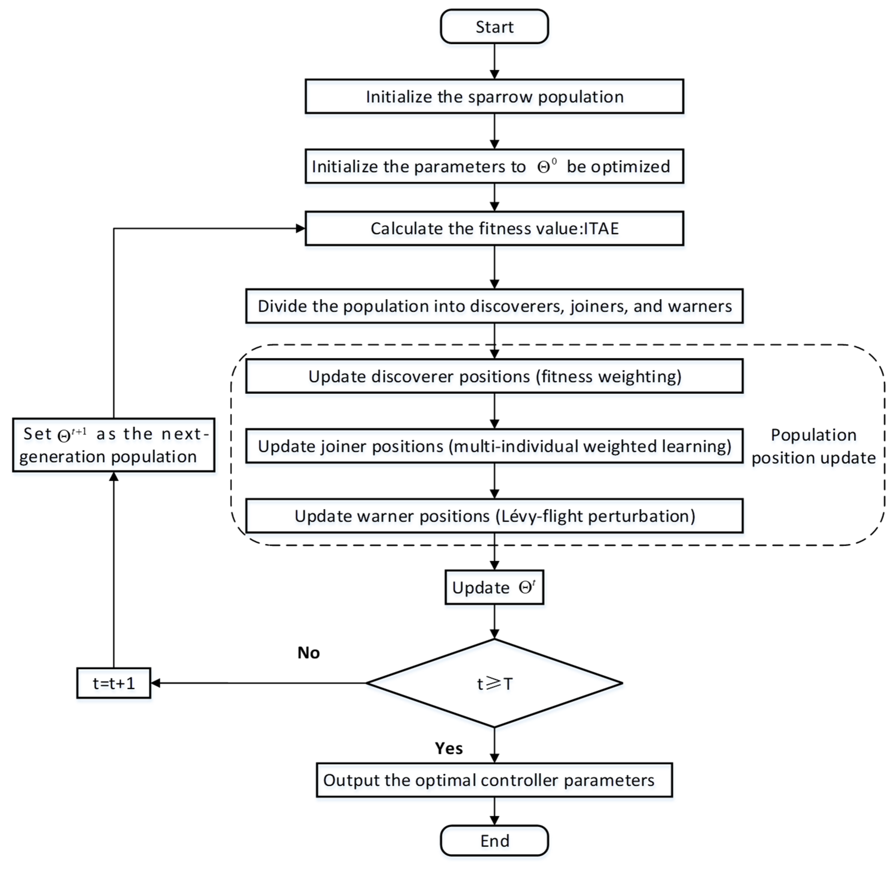
The multi-strategy fusion SSA proposed in Section 4.1 is used to optimize the composite-controller parameters. The parameters of the two fractional-order channel controllers are encoded into a single vector representing a sparrow’s position. Each candidate vector is substituted into the composite control system, the fitness corresponding to the two-channel tracking errors is calculated, and the population positions are updated according to fitness until the parameter combination minimizing the objective is obtained. The process is illustrated in the figure, and the detailed steps are as follows.

(1) Population initialization: Set the main algorithm parameters, including population size, maximum number of iterations, parameter dimension, producer proportion, sentinel proportion, and safety threshold $S$, and randomly generate the initial sparrow population.

As described above, fractional-order controllers $C_1(s)$ and $C_2(s)$ act on the two control channels. Each controller contains five parameters: proportional gain, integral gain, derivative gain, integral order, and derivative order. The two channels therefore contain ten parameters to be optimized, represented by the vector

$$\mathsf{\Theta }=[K_{p1},K_{i1},K_{d1},{\lambda }_1,{\mu }_1,K_{p2},K_{i2},K_{d2},{\lambda }_2,{\mu }_2]$$

(27)

where $K_{p1}, K_{i1}, K_{d1}, {\lambda }_1, {\mu }_1$ contains the parameters of fractional-order controller $C_1(s)$, and $K_{p2}, K_{i2}, K_{d2}, {\lambda }_2, {\mu }_2$ contains those of fractional-order controller $C_2(s)$.

The main parameters of the multi-strategy fusion SSA are listed in

Table 2. Parameter settings of the multi-strategy fusion SSA.

Parameter	Meaning	Value
$N$	Population size	100
$T$	Maximum number of iterations	100
$M$	Optimization dimension	10
$PD$	Producer proportion	0.7
$PA$	Sentinel proportion	0.3
$S$	Safety threshold	0.6

.

Because the parameters of two fractional-order controllers are optimized simultaneously, $M=10$. The position of sparrow $i$ is

$$X_i=[x_{i,1},x_{i,2},\dots ,x_{i,M}]$$

(28)

(2) Parameters to be optimized: In controller-parameter optimization, each sparrow $X_i$ corresponds to one candidate controller-parameter set:

$$X_i=[K_{p1,i},K_{i1,i},K_{d1,i},{\lambda }_{1,i},{\mu }_1,K_{p2,i},K_{i2,i},K_{d2,i},{\lambda }_{2,i},{\mu }_{2,i}]$$

(29)

where $i=1,2,\dots ,N$. During population initialization, the position of individual $i$ in dimension $j$ is randomly generated within the parameter bounds:

$$x_{i,j}=x_{j,\min }+\alpha (x_{j,\max }-x_{j,\min })$$

(30)

where $j=1,2,\dots ,M$; $X_{j,\min }$ and $X_{j,\max }$ are the lower and upper bounds, respectively, of optimization parameter $j$; and $\alpha \in [0,1]$ is a random number. This initialization ensures that every candidate parameter set lies within the prescribed search space.

(3) Fitness calculation: After population initialization, substitute the controller parameters represented by each sparrow into the composite control system, calculate the output response, and evaluate the fitness from the two-channel tracking errors. To assess response speed, tracking accuracy, and stability comprehensively, select the integral of time-weighted absolute error (ITAE) as the fitness criterion. For the two-channel beam-steering system, the objective function is

$$J={\displaystyle {\int }_0^{T}t(\left|e_x(t)\right|+\left|e_y(t)\right|)}dt$$

(31)

where $T$ is the simulation time, and $e_x(t)$ and $e_y(t)$ are the tracking errors in channels $x$ and $y$, respectively.

$$e_x(t)={\theta }_{ix}(t)-{\theta }_{ox}(t)$$

(32)

$$e_y(t)={\theta }_{iy}(t)-{\theta }_{oy}(t)$$

(33)

where ${\theta }_{ix}(t)$ and ${\theta }_{iy}(t)$ are the desired input deflection angles of the two channels, and ${\theta }_{ox}(t)$ and ${\theta }_{oy}(t)$ are the actual system output angles. Equation (30) shows that faster response, smaller tracking error, and shorter error duration produce a smaller objective $J$. The composite-controller optimization problem can therefore be formulated as

$${\mathsf{\Theta }}^{*}=\underset{\mathsf{\Theta }}{\arg \min }J(\mathsf{\Theta })$$

(34)

where ${\mathsf{\Theta }}^{*}$ is the optimized controller-parameter vector.

(4) Population ranking and role assignment: Rank the current population by fitness. A smaller fitness value indicates better response performance for the corresponding controller parameters. Determine the current global best position $X_{best}$ and global worst position $X_{worst}$, then divide the ranked population into producers, scroungers, and sentinels.

(5) Population position update: Update the positions of the three roles using the multi-strategy fusion SSA described in Section 4.1. Producers use fitness-weighted updates so that the search is directed more strongly toward high-fitness regions, improving global search. Scroungers use multi-individual weighted learning to exploit information from several good individuals and strengthen cooperative search. Sentinels use Levy-flight perturbations to expand the local search range and improve escape from local optima.

(6) Best-individual update: After updating the population positions, recalculate all fitness values and compare the current best individual with the historical best. If the current best is better, update the global optimum; otherwise, retain the historical optimum and update ${\mathsf{\Theta }}^t$.

(7) Termination test: Determine whether the current iteration has reached the maximum $T$ or the objective value satisfies the prescribed accuracy. If a termination condition is met, stop and output the optimal controller parameters. Otherwise, increment the iteration count by $t=t+1$, use the updated population as the next generation, and return to the fitness-calculation step.

(8) Output of the optimum: When a termination condition is met, output the optimal controller-parameter vector ${\mathsf{\Theta }}^{\ast }$ and its objective value. The resulting ${\mathsf{\Theta }}^{\ast }$ is the optimal composite-controller parameter combination used in the subsequent simulations and experiments.

As shown in Figure 8, the parameters of the two fractional-order channel controllers are first encoded as sparrow positions, and random initialization generates a population of candidate parameter sets. Each candidate is then substituted into the composite control system and evaluated using the two-channel ITAE index. Fitness ranking assigns the producer, scrounger, and sentinel roles, after which fitness weighting, multi-individual weighted learning, and Levy-flight perturbation update the population positions. Iterative comparison yields the global best individual and the optimal composite-controller parameters ${\mathsf{\Theta }}^{\ast }$.

The optimized composite-controller parameter vector is therefore

$${\mathsf{\Theta }}^{*}=[K_{p1}^{*},K_{i1}^{*},K_{d1}^{*},{\lambda }_1^{*},{\mu }_1^{*},K_{p2}^{*},K_{i2}^{*},K_{d2}^{*},{\lambda }_2^{*},{\mu }_2^{*}]$$

(35)

where $K_{p1}^{\ast }, K_{i1}^{\ast }, K_{d1}^{\ast }, {\lambda }_1^{\ast }, {\mu }_1^{\ast }$ contains the parameters of fractional-order controller $C_1(s)$, and $K_{p2}^{\ast }, K_{i2}^{\ast }, K_{d2}^{\ast }, {\lambda }_2^{\ast }, {\mu }_2^{\ast }$ contains those of fractional-order controller $C_2(s)$. The composite-controller parameters obtained using the multi-strategy fusion SSA are listed in

Table 3. Optimized composite-controller parameters.

Controller Parameters	Proportional Gain $K_p$	Integral Gain $K_i$	Derivative Gain $K_d$	Integral Order $\lambda$	Derivative Order $\mu$
$C_1(s)$	61.70	28.71	55.66	0.99	0.75
$C_2(s)$	66.75	27.99	69.86	0.99	0.85

.

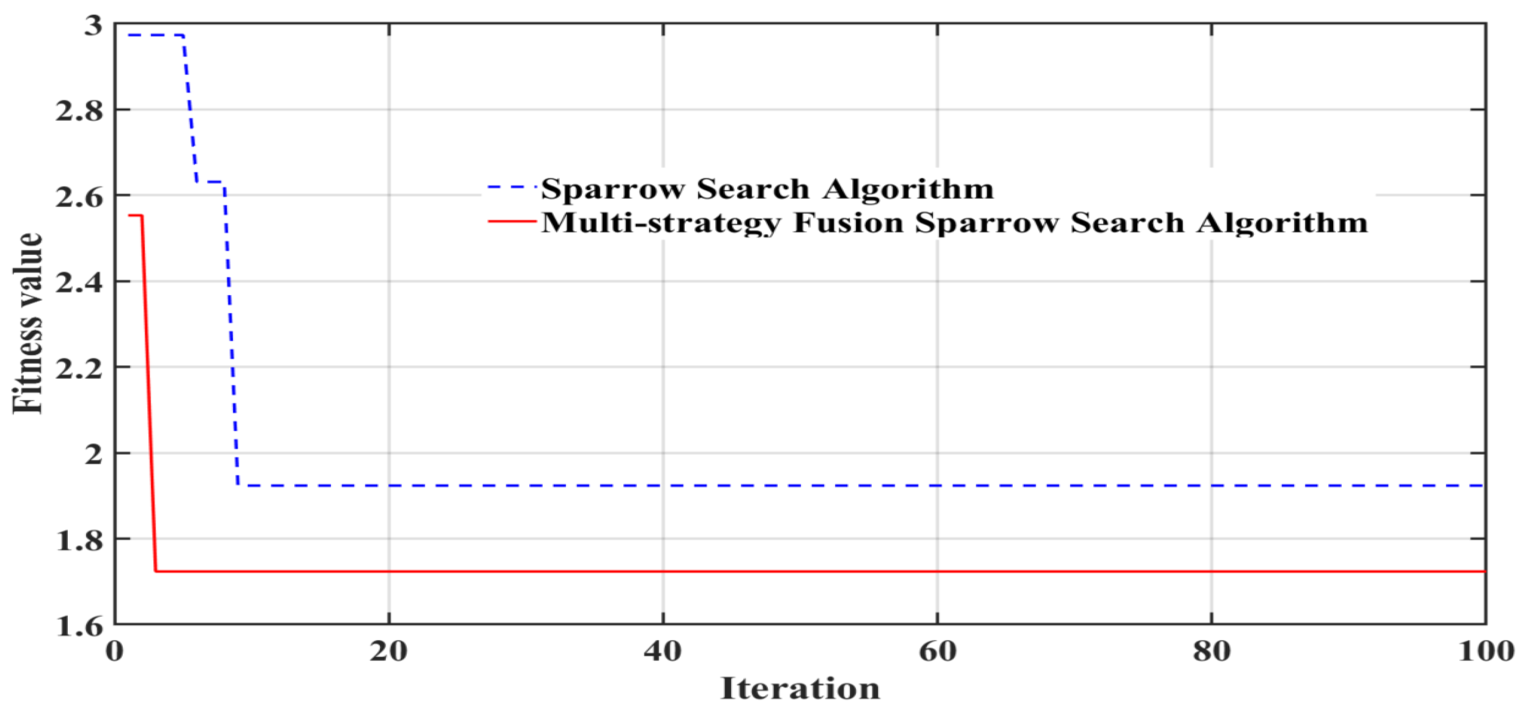
To further evaluate the convergence performance of the multi-strategy fusion sparrow search algorithm, the proposed algorithm is compared with the standard sparrow search algorithm under identical population size, number of iterations, parameter search ranges, and fitness function settings. The corresponding fitness convergence curves are shown in Figure 9.

As can be seen from Figure 9, the fitness value of the multi-strategy fusion sparrow search algorithm decreases rapidly during the early iterations and converges within fewer iterations, whereas the standard sparrow search algorithm exhibits a relatively slower convergence rate. Moreover, the proposed algorithm achieves a lower final fitness value than does the standard sparrow search algorithm, indicating that the introduced multi-strategy collaborative update mechanism can improve both the convergence speed and the optimization capability of the algorithm.

To further evaluate the offline computational cost of the multi-strategy fusion sparrow search algorithm, the runtime, total number of objective-function evaluations, and memory usage during the complete parameter optimization process were recorded. With a population size of 100 and a maximum of 100 iterations, one complete parameter optimization required approximately 42.43 min, with a total of 10,100 objective-function evaluations and a peak memory usage of approximately 68.02 MB. It should be noted that this optimization process is used only for offline tuning of the fractional-order controller parameters and is not involved in the actual online closed-loop control. Therefore, its computational cost does not directly affect the real-time control performance of the system.

5. Closed-Loop Stability Analysis of the Beam-Steering System Based on Closed-Loop Characteristic Roots

As described in Section 3.1, the beam-steering system designed in this study adopts a composite control architecture consisting of fractional-order controllers, a diagonal decoupling compensator, and a Smith predictor. The diagonal decoupling compensator approximately decouples the two-input two-output coupled system into two independent main control channels, while the Smith predictor further mitigates the influence of pure time delay on closed-loop stability. Therefore, based on the decoupling compensation and Smith predictor compensation, the closed-loop characteristic equations of the X- and Y-axis main channels are established separately in this section, and the system stability is analyzed through the distribution of the closed-loop characteristic roots.

5.1. Derivation of the Fractional-Order Closed-Loop Characteristic Equation

According to the diagonal decoupling compensator designed in Section 3.2, the equivalent plant of the decoupled X-axis channel can be expressed as

$$G_x(s)=G_{11}(s)-G_{12}(s)D_{21}(s)$$

(36)

The equivalent plant of the decoupled Y-axis channel can be expressed as

$$G_y(s)=G_{22}(s)-G_{21}(s)D_{12}(s)$$

(37)

Considering the time-delay elements present in the system, the actual plants in the X- and Y-axis directions can be expressed as

$$\begin{array}{l}{G}_{x\tau }(s)=G_x(s)e^{-{\tau }_{x}s}\\ G_{y\tau }(s)=G_y(s)e^{-{\tau }_{y}s}\end{array}$$

(38)

For the X-axis main control channel, its open-loop transfer function can be expressed as

$${\theta }_{ax}(s)=(G_{11}(s)-G_{12}(s)D_{21}(s))\Delta {\phi }_x(s)$$

(39)

The corresponding closed-loop transfer function can be expressed as

$${\displaystyle \frac{{\theta }_{ax}(s)}{{\theta }_{ix}(s)}}={\displaystyle \frac{C_1(s)G_x(s)}{1+C_1(s)G_x(s)}}$$

(40)

Therefore, the closed-loop characteristic equation of the X-axis channel can be expressed as

$$1+C_1(s)G_x(s)=0$$

(41)

Similarly, the open-loop transfer function of the Y-axis main control channel can be expressed as

$${\theta }_{yx}(s)=(G_{22}(s)-G_{21}(s)D_{12}(s))\Delta {\phi }_y(s)$$

(42)

The closed-loop transfer function can be expressed as

$${\displaystyle \frac{{\theta }_{ay}(s)}{{\theta }_{iy}(s)}}={\displaystyle \frac{C_2(s)G_y(s)}{1+C_2(s)G_y(s)}}$$

(43)

Therefore, the closed-loop characteristic equation of the Y-axis channel can be expressed as

$$1+C_2(s)G_y(s)=0$$

(44)

If the equivalent decoupled plant is uniformly expressed as

$$C_i(s)={\displaystyle \frac{K_i}{{\eta }_1{s}^{\alpha }+{\eta }_2{s}^{\beta }+\mu s^{\gamma }+k}}i=x,y$$

(45)

where $K_i$ denotes the system gain, substituting the fractional-order controller designed in Section 3.1 into the characteristic equation yields

$$1+(K_{p_i}+K_{i_i}{s}^{-{\lambda }_i}+K_{d_i}{s}^{{\mu }_i}){\displaystyle \frac{K_i}{{\eta }_1{s}^{\alpha }+{\eta }_2{s}^{\beta }+\mu s^{\gamma }+k}}=0$$

(46)

After rearrangement, it can be expressed as

$${\eta }_1{s}^{\alpha }+{\eta }_2{s}^{\beta }+\mu s^{\gamma }+k+K_i{K}_{p_i}+K_i{K}_{i_i}{s}^{-{\lambda }_i}+K_i{K}_{d_i}{s}^{{\mu }_i}=0$$

(47)

For convenience in analyzing the closed-loop characteristic roots, both sides are multiplied by $s^{{\lambda }_i}$ to eliminate the negative-order term, yielding the following fractional order closed-loop characteristic equation:

$${\eta }_1{s}^{\alpha +{\lambda }_i}+{\eta }_2{s}^{\beta +{\lambda }_i}+\mu s^{\gamma +{\lambda }_i}+(k+K_i{K}_{p_i})s^{{\lambda }_i}+K_i{K}_{d_i}{s}^{{\mu }_i+{\lambda }_i}+K_i{K}_{i_i}=0$$

(48)

when $i=x$, the above equation represents the closed-loop characteristic equation of the X-axis channel; when $i=y$, it represents the closed-loop characteristic equation of the Y-axis channel.

5.2. Stability Analysis Based on the Matignon Criterion

For a fractional-order closed-loop system, its stability can be determined using the Matignon stability criterion. The fractional orders in the closed-loop characteristic equation are uniformly expressed as integer multiples of a common base order $q$, where $0<q<2$. If all characteristic roots $p_i$ of the closed-loop system satisfy

$$\left|\arg (p_i)\right|>{\displaystyle \frac{q\pi }{2}}$$

(49)

then the system is asymptotically stable.

To further verify the closed-loop stability of the designed controller with the actual parameter settings, the identified plant models and controller parameters of the X- and Y-axis channels are subsequently substituted into their respective closed-loop characteristic equations. The closed-loop characteristic roots are then calculated, and the system stability is analyzed according to the Matignon stability criterion.

5.3. Closed-Loop Characteristic Root Stability Verification for the X-Axis Channel

Substituting the plant parameters given in Section 2 and the optimized fractional-order controller parameters obtained in Section 4 into Equation (48), the closed-loop characteristic equation of the X-axis channel can be obtained after rearrangement as

$$s^{2.88}+1.0621s^{1.97}+1.4082\times {10}^{-7}{s}^{1.04}+0.3970s^{0.99}+3.8507\times {10}^{-12}+7.4653\times {10}^{-12}{s}^{1.74}=0$$

(50)

Since the terms in the closed-loop characteristic equation have different fractional orders, all fractional exponents are expressed in terms of a common base order to facilitate stability analysis using the Matignon stability criterion. The common base order is chosen as

$$q=0.01$$

(51)

Let:

$$z=s^{0.01}$$

(52)

Then, the closed-loop characteristic equation of the X-axis channel can be transformed into

$$z^{288}+1.0621z^{197}+1.4082\times {10}^{-7}{z}^{104}+0.3970z^{99}+3.8507\times {10}^{-12}{z}^0+7.4653\times {10}^{-12}{z}^{174}=0$$

(53)

The above characteristic equation is solved using MATLAB R2024a to obtain all the characteristic roots of the X-axis closed-loop system. To avoid listing all the characteristic roots individually, the characteristic root closest to the Matignon stability boundary is selected as the basis for stability assessment. The results show that the characteristic root with the minimum absolute phase angle in the X-axis closed-loop system is

$$p_{x,\min }=0.9934+0.0265i$$

(54)

Its phase angle is given by

$$\left|\arg (p_{x,\min })\right|=1.5288\mathrm{deg}$$

(55)

The relationship between the phase angle of this characteristic root and the Matignon stability boundary is given by

$$\left|\arg (p_{x,\min })\right|>{\displaystyle \frac{0.01\pi }{2}}=0.9\mathrm{deg}$$

(56)

Since $p_{x,\min }$ is the characteristic root closest to the stability boundary among all the characteristic roots, all the closed-loop characteristic roots of the X-axis channel satisfy the Matignon stability criterion.

5.4. Closed-Loop Characteristic Root Stability Verification for the Y-Axis Channel

Similarly, substituting the plant parameters given in Section 2 and the optimized fractional-order controller parameters obtained in Section 4 into Equation (48), the closed-loop characteristic equation of the Y-axis channel can be obtained after rearrangement as

$$s^{2.88}+1.0621s^{1.97}+1.4082\times {10}^{-7}7s^{1.04}+0.3970s^{0.99}+3.7483\times {10}^{-12}+9.3554\times {10}^{-12}{s}^{1.84}=0$$

(57)

Following the same common-base-order transformation procedure as that used for the X-axis channel, the closed-loop characteristic equation of the Y-axis channel can be transformed into

$$z^{288}+1.0621z^{197}+1.4082\times {10}^{-7}{z}^{104}+0.3970z^{99}+3.7483\times {10}^{-12}{z}^0+9.3554\times {10}^{-12}{z}^{184}=0$$

(58)

The above characteristic equation is solved using MATLAB to obtain all the characteristic roots of the Y-axis closed-loop system, among which the characteristic root closest to the Matignon stability boundary is

$$p_{y,\min }=0.9934+0.0265i$$

(59)

Its phase angle is given by

$$\left|\arg (p_{y,\min })\right|=1.5288\mathrm{deg}$$

(60)

The phase angle of this characteristic root also satisfies the Matignon stability criterion, as follows:

$$\left|\arg (p_{y,\min })\right|>{\displaystyle \frac{0.01\pi }{2}}=0.9\mathrm{deg}$$

(61)

Therefore, all the closed-loop characteristic roots of the Y-axis channel satisfy the Matignon stability criterion. All characteristic roots of the Y-axis closed-loop system lie within the Matignon stability region, indicating that the Y-axis closed-loop system is asymptotically stable.

Based on the stability verification of the closed-loop characteristic roots for both the X- and Y-axis channels, it can be concluded that the two decoupled main control channels both satisfy the Matignon stability criterion, with all closed-loop characteristic roots located within the corresponding stability region. This demonstrates that the proposed fractional-order composite control system satisfies the closed-loop stability requirements.

6. Simulation Analysis of Beam-Steering Control Performance

To verify the effectiveness of the proposed composite strategy for LCOPA beam steering, comparative simulations are conducted for integer-order PID control, fractional-order PID control, active disturbance rejection control (ADRC) and the proposed composite control. Integer-order PID serves as the conventional baseline; fractional-order PID reveals the improvement obtained from fractional calculus operators; and the proposed composite method further adds diagonal decoupling and Smith predictor compensation to fractional-order control to weaken two-axis channel coupling and reduce the effect of system delay. With the plant model, input command, simulation duration, and initial conditions held constant, the outputs of the four methods are compared using settling time, overshoot, and steady-state error to evaluate dynamic response and steady-state accuracy.

The dynamic response, steady-state accuracy, and decoupling capability of the proposed strategy are comprehensively evaluated in terms of settling time, overshoot, steady-state error, and coupling suppression. The additional deflection of the non-commanded channel under a single-channel input is used to compare suppression of two-axis coupling, and parameter perturbations are introduced to further evaluate robustness and stability.

6.1. Simulation Model and Comparative Schemes

The LCOPA beam-steering dynamic model established in Section 2 is used as the plant, and four closed-loop systems are constructed: PID control, fractional-order PID control, ADRC and the proposed composite control.

To ensure a fair comparison, all simulations use the same plant model, target input, initial conditions, simulation duration, and numerical solution settings. The parameters of all four controllers are optimized using the multi-strategy fusion SSA proposed in Section 4, with the two-channel ITAE as the fitness function. The same population size, maximum iteration count, and algorithm settings are used for all methods, while the optimization dimension is selected according to each controller structure.

For the integer-order PID controller, the integral and derivative orders are fixed at $\lambda =1$ and $\mu =1$, and only the proportional, integral, and derivative gains of the two channels are optimized. For the fractional-order PID controller, the proportional gain $K_p$, integral gain $K_i$, derivative gain $K_d$, integral order $\lambda$, and derivative order $\mu$ are optimized simultaneously. The optimization procedure and final parameters of the fractional-order part of the proposed composite controller were given in Section 4.2 and are listed in Table 2. To avoid repetition, this section reports only the optimized parameters of the integer-order PID and fractional-order PID baselines, as shown in

Table 4. Optimized parameters of the PID and FOPID controllers.

Control Method	Control Channel	Proportional Gain $K_p$	Integral Gain $K_i$	Derivative Gain $K_d$	Integral Order $\lambda$	Derivative Order $\mu$
PID controller	$C_1(s)$	10.65	6.84	9.76	1	1
	$C_2(s)$	10.86	6.78	9.77	1	1
FOPID controller	$C_1(s)$	24.30	8.99	30.81	1.01	0.88
	$C_2(s)$	23.60	8.48	28.80	1.01	0.95

.

For the ADRC benchmark, second-order linear ADRC controllers are employed separately for the X- and Y-axis control channels, each equipped with a third-order linear extended state observer (LESO). The ADRC parameters are determined using the bandwidth parameterization method. The controller gains satisfy $k_p=w_c^2$ and $k_d=2w_c$, while the observer gains satisfy ${\beta }_1=2w_c$, ${\beta }_2=3w_0^2$ and ${\beta }_3=w_0^2$. Different controller bandwidths and observer bandwidths are adopted for the two control channels, and the specific parameter values are listed in

Table 5. ADRC controller parameter settings.

Control Channel	${\mathit{w}}_{\mathit{c}}$	${\mathit{w}}_{\mathit{o}}$	${\mathit{k}}_{\mathit{p}}$	${\mathit{k}}_{\mathit{d}}$	${\mathit{\beta }}_{\mathbf{1}}$	${\mathit{\beta }}_{\mathbf{2}}$	${\mathit{\beta }}_{\mathbf{3}}$
$C_1(s)$	19	70	361	38	210	14,700	343,000
$C_2(s)$	20	72	400	40	216	15,552	373,248

.

6.2. Comparative Simulation of Step-Response Performance

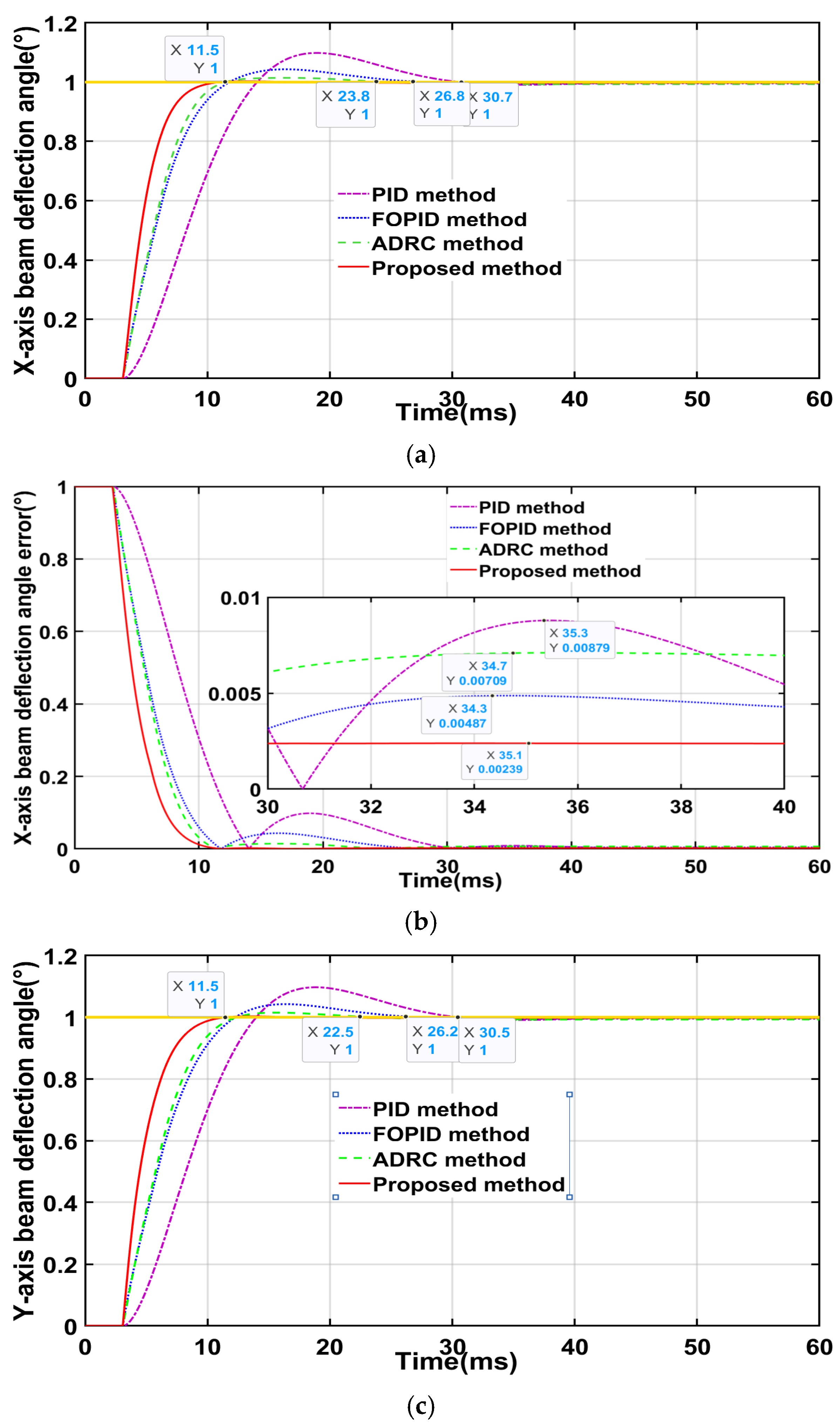
To verify the improvement in dynamic response and steady-state accuracy provided by the proposed composite method, 1° step commands are applied to the X- and Y-axis control channels, and integer-order PID, fractional-order PID, ADRC and the proposed composite control are compared.

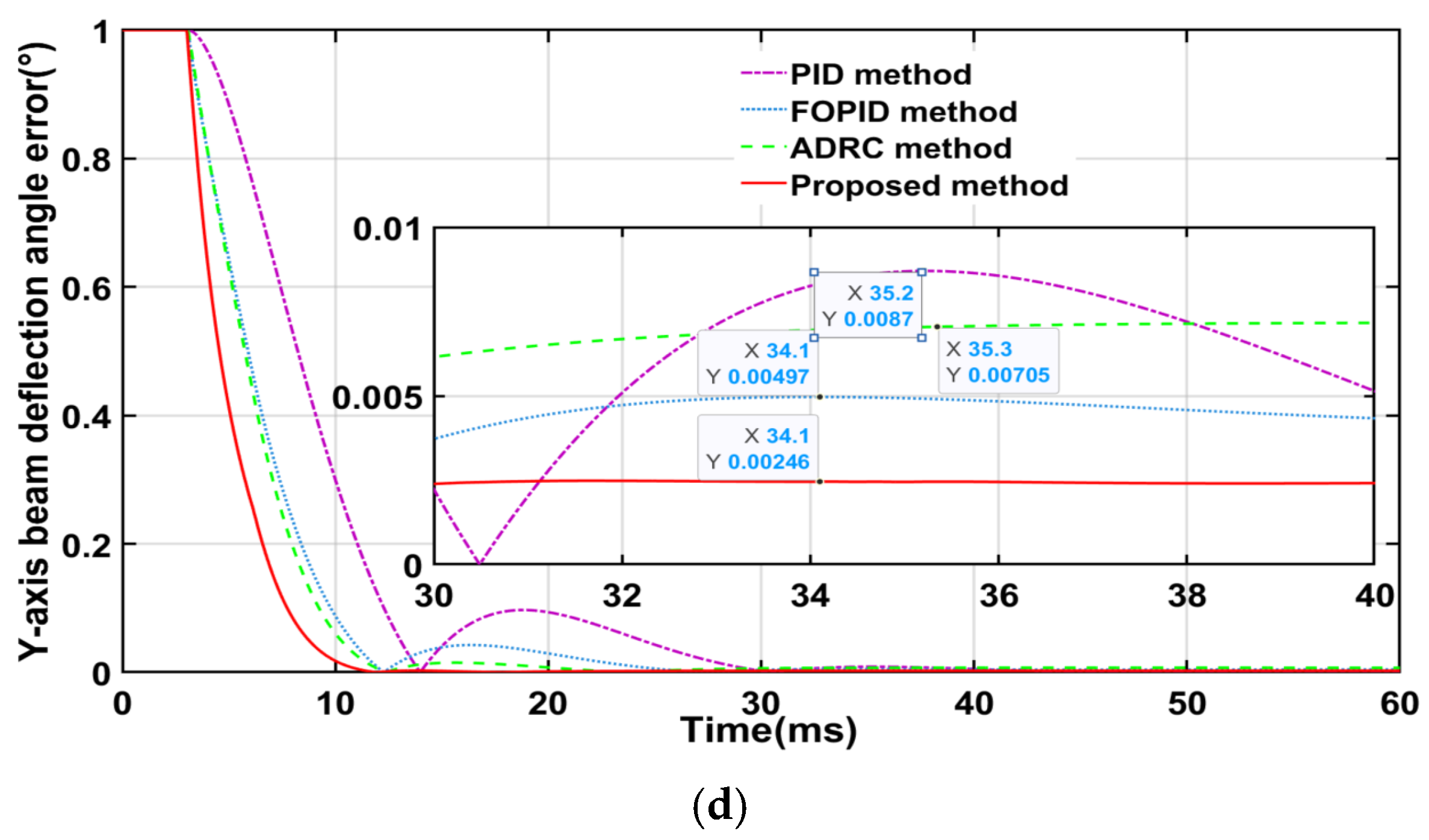
Figure 10 shows that all four methods stably track the target X- and Y-axis deflection angles, but their dynamic performance differs substantially. PID control responds slowly and exhibits relatively large overshoot and a long error-decay process. By adding adjustable integral and derivative orders, FOPID control improves response speed and overshoot suppression relative to that of PID. ADRC further shortens the system response time and reduces the overshoot, demonstrating good dynamic response performance. In contrast, the proposed composite method tracks the target angle more rapidly in both channels, with virtually no visible oscillation, and its tracking errors decay quickly to low levels. The consistent X- and Y-axis results indicate that the proposed method simultaneously improves speed, stability, and accuracy in two-axis beam steering.

For a quantitative comparison, the settling time, overshoot, and steady-state error of the four methods are summarized in

Table 6. Comparison of step-response performance indices under different control methods.

Control Method	Control Channel	Settling Time (ms)	Overshoot (%)	Steady-State Error (°)
PID method	X-axis	30.70	9.82%	8.79 × 10−3
	Y-axis	30.50	9.70%	8.70 × 10−3
FOPID method	X-axis	26.80	4.33%	7.10 × 10−3
	Y-axis	26.20	4.25%	7.05 × 10−3
ADRC method	X-axis	23.80	1.44%	4.87 × 10−3
	Y-axis	22.50	1.50%	4.97 × 10−3
Proposed method	X-axis	11.50	0.22%	2.38 × 10−3
	Y-axis	11.50	0.26%	2.46 × 10−3

.

As shown in Table 6, the proposed composite control method achieves a settling time of 11.50 ms for both the X- and Y-axes, significantly outperforming PID, FOPID, and ADRC. Compared with the results for PID, FOPID, and ADRC, the settling time of the X-axis is reduced by 62.54%, 57.09%, and 51.68%, respectively, while that of the Y-axis is reduced by 62.30%, 56.11%, and 48.89%, respectively. Meanwhile, the overshoot of both axes is below 0.3%, and the steady-state errors remain on the order of 10⁻³, with both outperforming the other results for the comparative methods. These results demonstrate that the proposed method can effectively reduce overshoot and steady-state error while improving the system response speed, thereby exhibiting superior overall control performance.

6.3. Simulation Analysis of Decoupling Performance

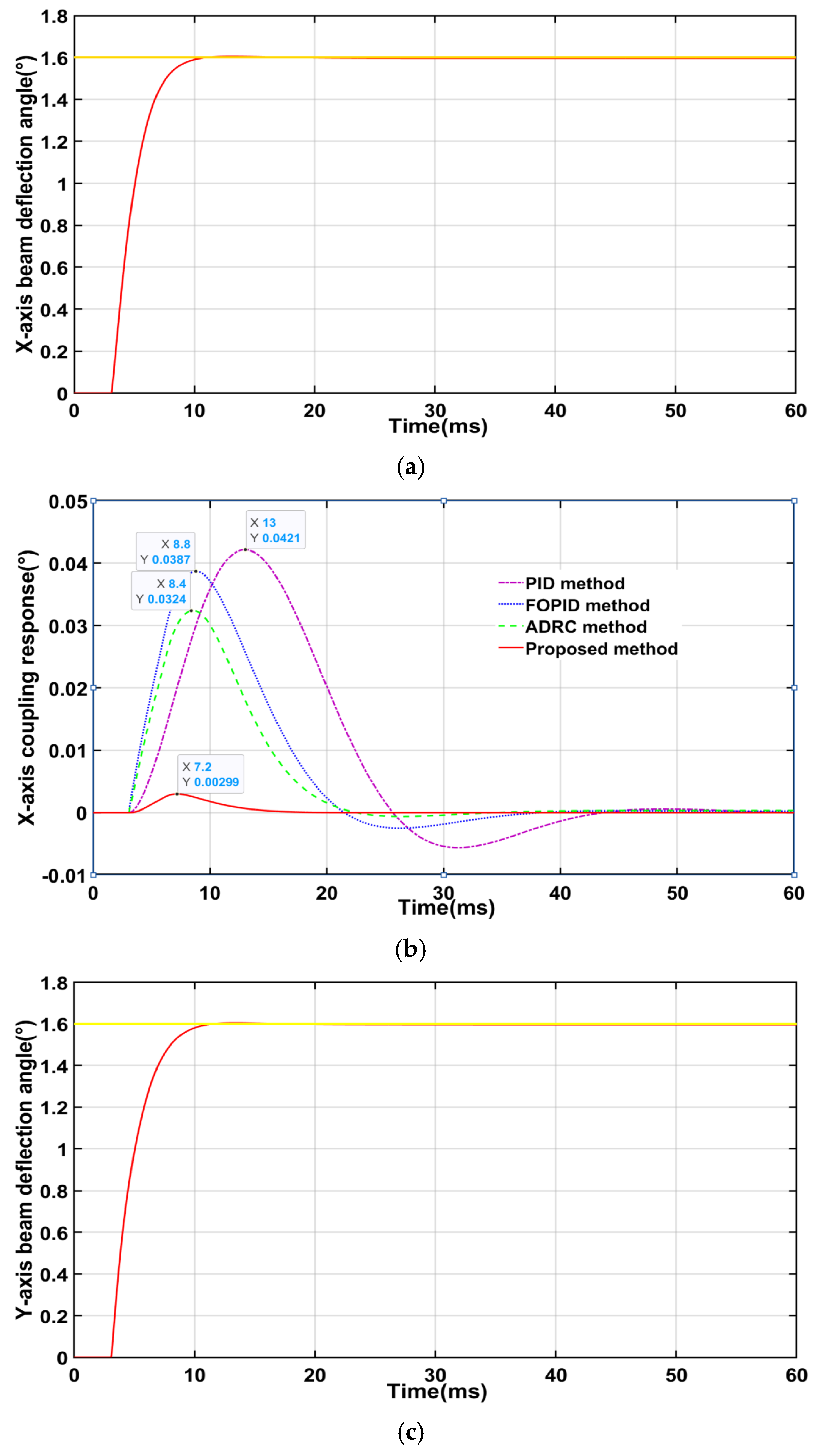
To verify suppression of two-axis channel coupling, single-channel step simulations are performed for both axes. In the X-axis test, the X-axis target is 1.6°, and the Y-axis target is 0°; the X-axis response and Y-axis coupled response are recorded. In the Y-axis test, the Y-axis target is 1.6°, and the X-axis target is 0°; the Y-axis response and X-axis coupled response are recorded. Coupling suppression is compared among PID, FOPID, ADRC and the proposed composite method.

Figure 11a,c show that, for a 1.6° step command applied to either axis, the proposed method stably tracks the target deflection angle in the commanded channel and does not introduce an appreciable steady-state bias through the decoupling compensator. The designed decoupling structure therefore compensates the coupling terms without degrading channel-tracking performance.

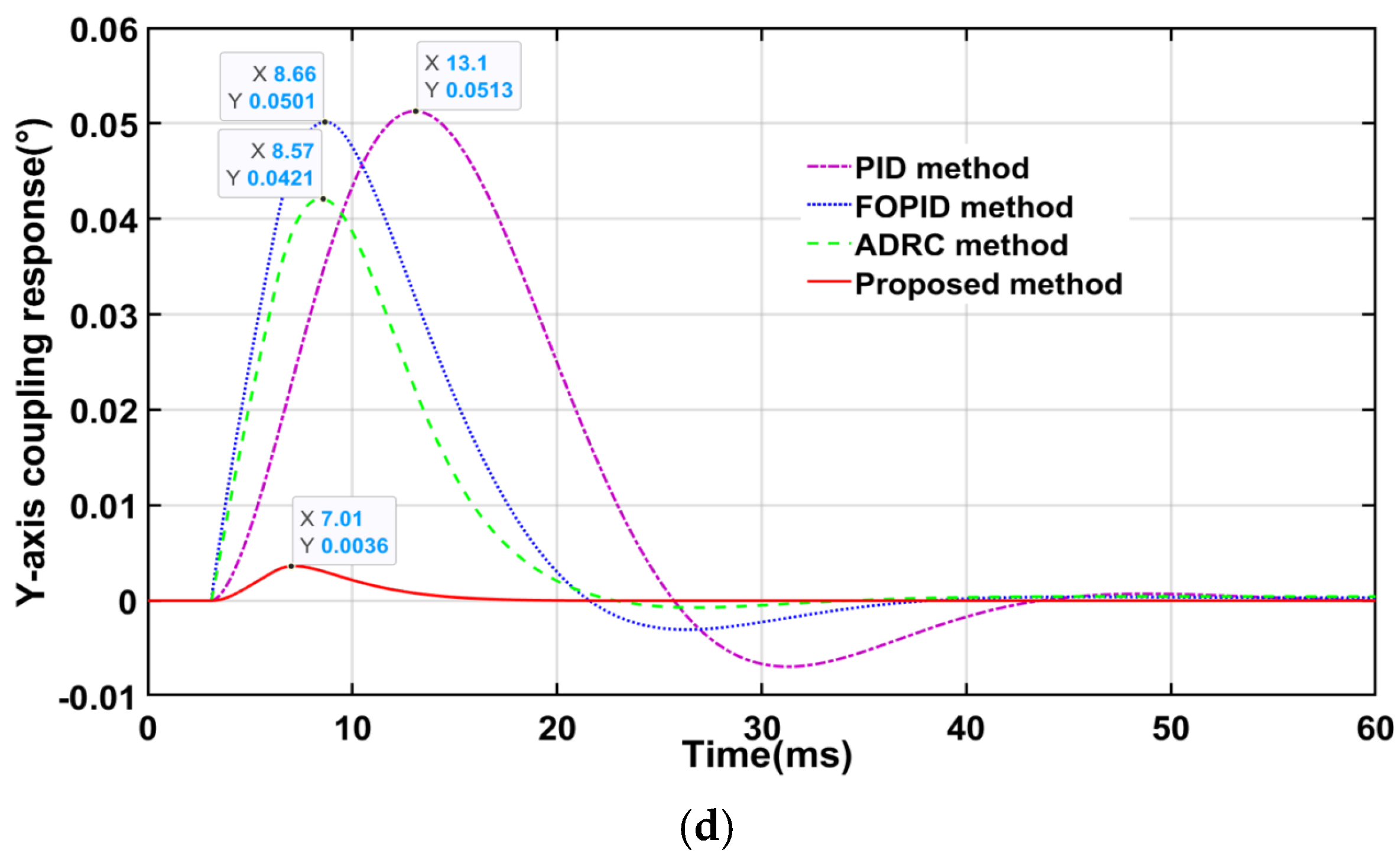
The channel responses in Figure 11b,d show that both PID and FOPID control cause an appreciable transient deflection of the non-commanded axis during single-axis steering. PID produces a larger coupling peak and slower decay. FOPID reduces the coupling amplitude to some extent, but noticeable coupled fluctuations remain. ADRC further reduces the peak coupling response, demonstrating good disturbance rejection capability. By comparison, the proposed composite method significantly reduces the coupling peaks in both directions and returns them close to zero within a short time, demonstrating that the diagonal decoupling compensator effectively weakens cross-coupling between the two axis channels.

For further quantitative evaluation, the maximum Y-axis coupling caused by an X-axis input, the maximum X-axis coupling caused by a Y-axis input, and the corresponding coupling ratios are summarized in

Table 7. Comparison of two-axis coupling suppression under different control methods.

Control Method	X-to-Y Coupling Amplitude (°)	X-to-Y Coupling Ratio (%)	Y-to-X Coupling Amplitude (°)	Y-to-X Coupling Ratio (%)
PID method	0.0513	3.21	0.0421	2.63
FOPID method	0.0501	3.13	0.0387	2.42
ADRC method	0.0421	2.63	0.0324	2.03
Proposed method	0.0036	0.23	0.0030	0.19

.

Table 7 shows that under PID control, the maximum X-to-Y and Y-to-X coupling amplitudes are 0.0513° and 0.0421°, corresponding to coupling ratios of 3.21% and 2.63%, respectively. FOPID reduces the two-axis coupling response to some extent, but the improvement is limited. ADRC further reduces the maximum coupling deviations in the two directions to 0.0421° and 0.0324°, corresponding to coupling degrees of 2.63% and 2.03%, respectively, indicating its capability to suppress disturbances induced by channel coupling. With the proposed composite method, the maximum coupling amplitudes fall to 0.0036° and 0.0030°, and the corresponding coupling ratios are only 0.23% and 0.19%, respectively, significantly lower than those of the other three control methods, demonstrating that the designed diagonal decoupling compensator can effectively suppress the coupling effects between the two axes.

6.4. Simulation Analysis of Robustness to Disturbances

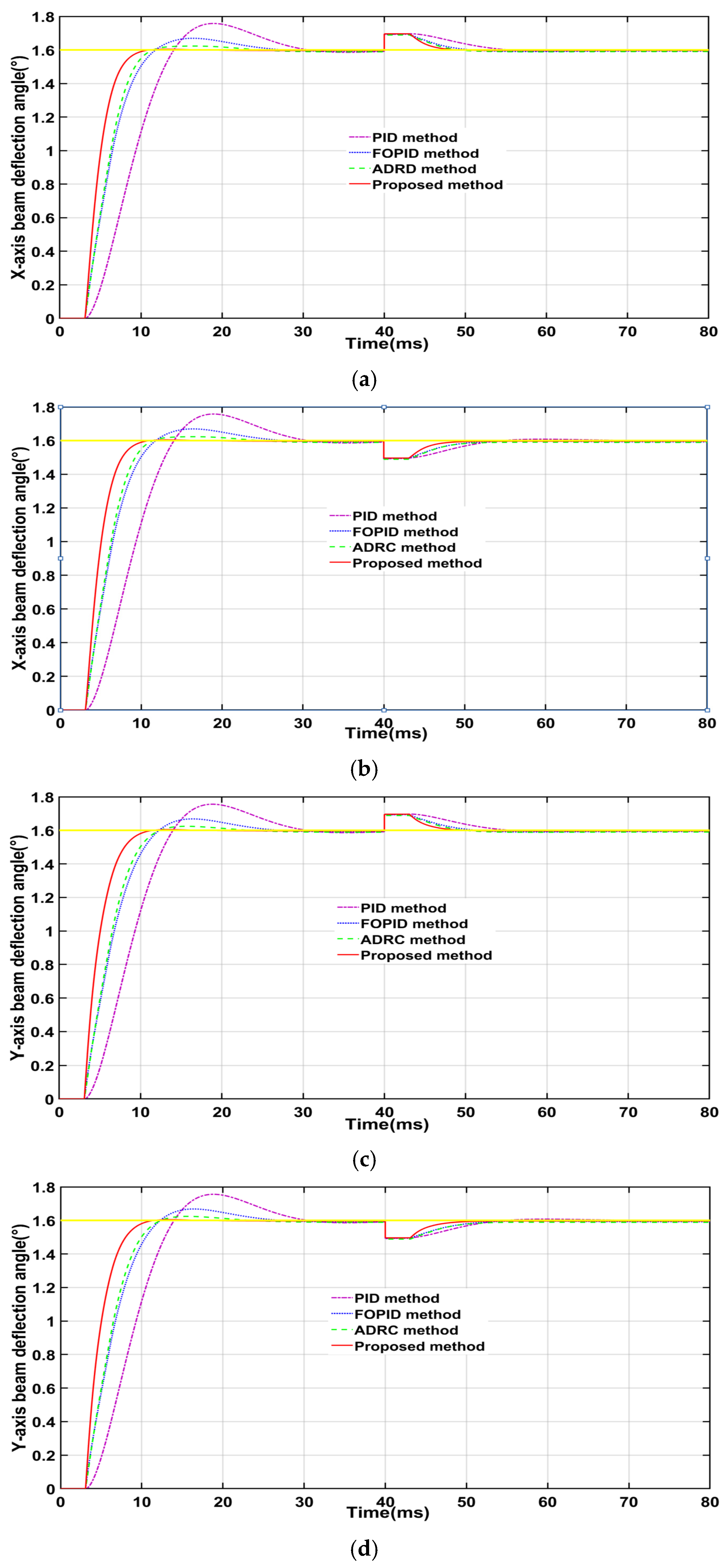
To verify robustness to external disturbances, the target deflection angle is held at 1.6°, and step disturbances of +0.1° and −0.1° are applied separately to the X- and Y-axis channels at 40 ms. The disturbance responses under PID, FOPID, ADRC and the proposed composite control are compared in Figure 12.

Figure 12 shows that all four methods stably track the target angle before the disturbance is applied. After the step disturbance, PID control produces a pronounced transient deviation and a relatively long recovery. FOPID reduces the disturbance-induced fluctuation, but a transient error of appreciable magnitude remains. ADRC estimates and compensates for disturbances, further reducing the output deviation caused by external disturbances and demonstrating good disturbance rejection performance. In contrast, the proposed composite method produces smaller output deviations in both channels and for both disturbance directions; the induced pointing error decays rapidly without visible recovery oscillation. The proposed method therefore effectively suppresses the effect of abrupt external disturbances on beam deflection and provides good disturbance rejection and pointing stability.

6.5. Ablation Analysis of the Composite Control Structure

To further investigate the contribution of each functional module in the proposed composite control structure to the overall system performance, four control configurations, namely FOPID, FOPID + Decoupling, FOPID + Smith, and FOPID + Decoupling + Smith, were constructed and evaluated under identical simulation conditions. 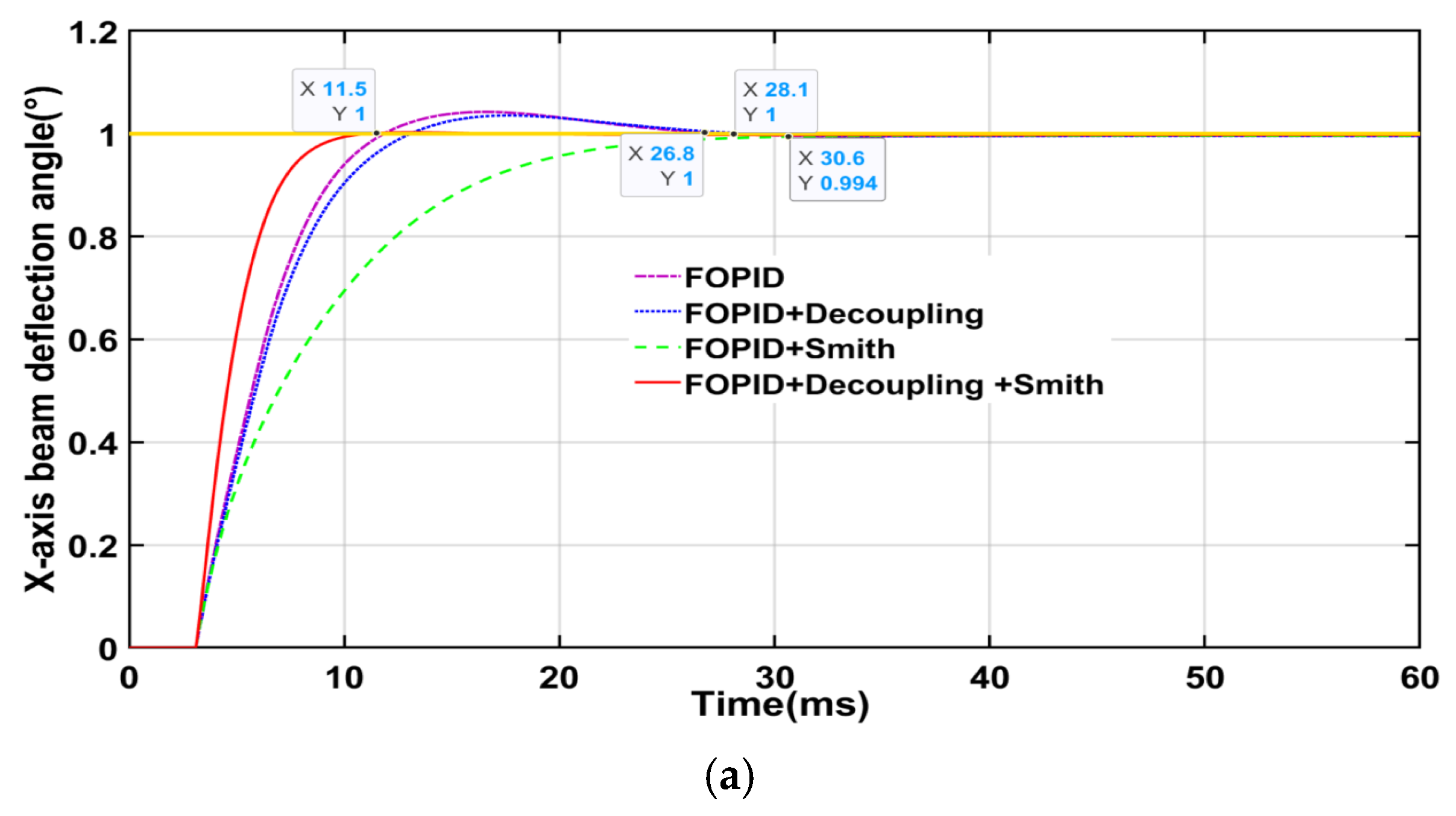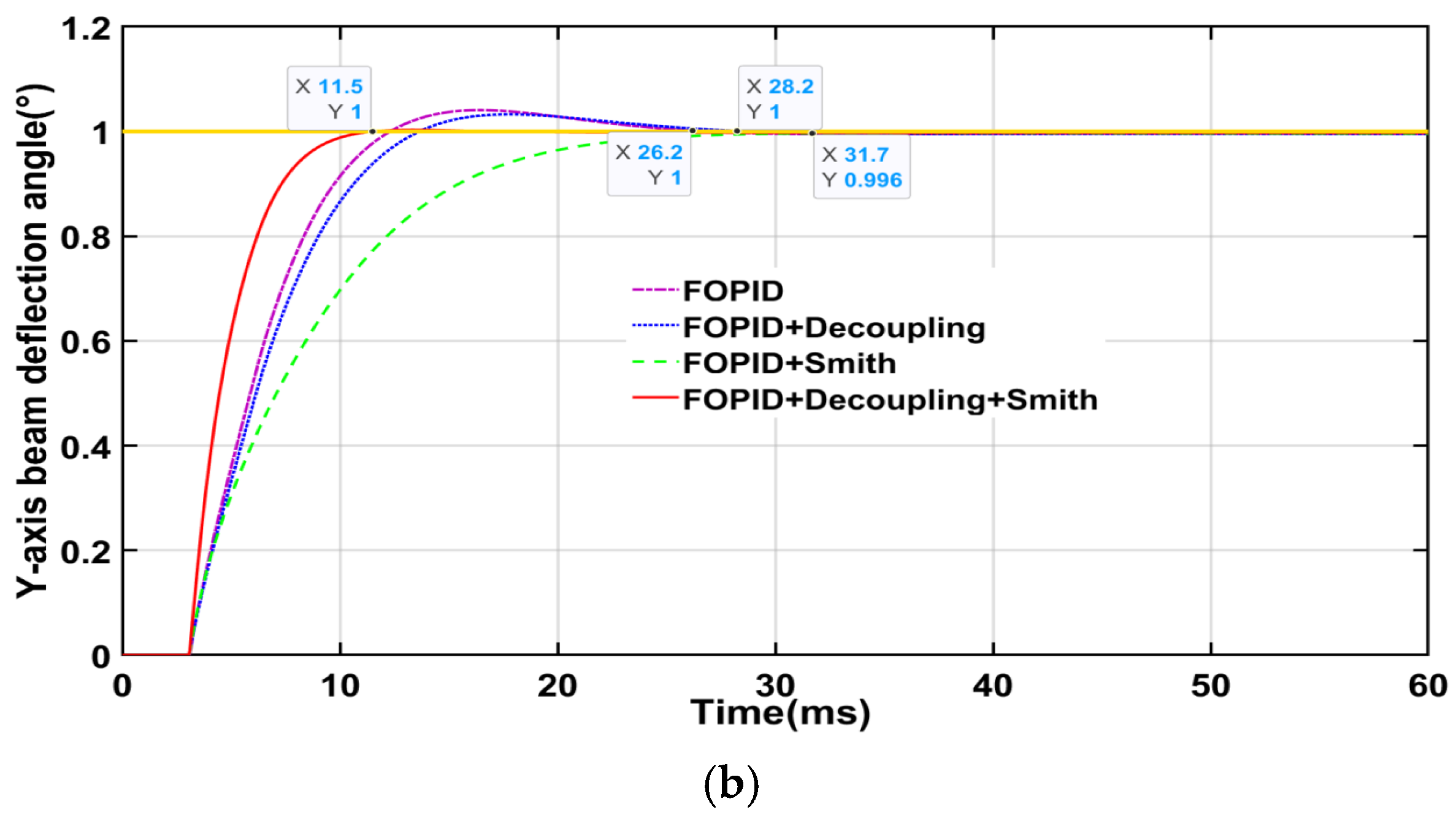Among them, FOPID serves as the baseline controller to regulate the main-channel dynamic characteristics; the diagonal decoupling compensator is employed to suppress the cross-coupling between the X- and Y-axis channels; and the Smith predictor is introduced to mitigate the adverse effects of system time delay on the closed-loop dynamic performance. By comparing the dynamic responses, steady-state errors, and maximum coupling deviations of the different control structures, the relative contribution of each functional module and their synergistic effects are evaluated. The dual-axis step responses under different control structures are shown in Figure 13.

As shown in Figure 13, the introduction of different compensation modules has a noticeable influence on the system dynamic response. When only FOPID control is employed, both the X- and Y-axis responses exhibit a certain amount of overshoot and require a relatively long time to reach steady state. After introducing the diagonal decoupling compensator, the overshoot and steady-state error are reduced, while the settling time changes only slightly, indicating that the primary role of the decoupling compensator is not to accelerate the main-channel response, but rather to suppress the cross-coupling between the two axes. With the Smith predictor introduced, the overshoot of both axes is nearly eliminated, and the steady-state error is further reduced, although the settling time increases. This indicates that the Smith predictor improves the closed-loop response characteristics in the presence of time delay, but does not achieve the best overall dynamic performance when used alone. When both the diagonal decoupling compensator and the Smith predictor are incorporated, faster responses and smaller steady-state errors are achieved for both the X- and Y-axis channels, demonstrating the synergistic effect of the different functional modules. To further quantitatively compare the performance of the different control structures, the settling time, overshoot, steady-state error, and maximum coupling deviation are summarized in

Table 8. Comparison of ablation simulation results for different control structures.

Control Scheme	Control Channel	Settling Time (ms)	Overshoot (%)	Steady-State Error (°)	Maximum Coupling Deviation (°)
FOPID	X-axis	26.80	4.33%	7.10 × 10−3	0.0501
	Y-axis	26.20	4.25%	7.05 × 10−3	0.0387
FOPID + Decoupling	X-axis	28.10	3.56%	4.73 × 10−3	0.0001
	Y-axis	28.20	3.28%	4.71 × 10−3	0.0001
FOPID + Smith	X-axis	31.60	0.00%	3.40 × 10−3	0.0292
	Y-axis	31.70	0.00%	3.31 × 10−3	0.0300
FOPID + Decoupling + Smith	X-axis	11.50	0.22%	2.38 × 10−3	0.0036
	Y-axis	11.50	0.26%	2.46 × 10−3	0.0030

.

As shown in Table 8, the diagonal decoupling compensator significantly reduces the maximum coupling deviation between the two axes, while the Smith predictor improves the overshoot and steady-state performance of the system. With the complete composite control structure, the settling times of both the X- and Y-axis channels are 11.50 ms, the steady-state errors are 2.38 × 10⁻³ and 2.46 × 10⁻³, respectively, and the maximum coupling deviations are 0.0036° and 0.0030°, respectively. The results demonstrate that the individual functional modules contribute differently to performance improvement, and their coordinated design achieves a favorable overall balance among dynamic response, steady-state accuracy, and coupling suppression.

7. Experimental Validation of the Beam-Steering System

To validate the proposed strategy on an actual LCOPA beam-steering system, a test platform is constructed, and experiments on decoupling and robustness are performed. Pointing accuracy is evaluated from the error between the actual and target deflection angles. External disturbances are also introduced to analyze changes in pointing error and verify system stability and robustness.

7.1. Experimental Platform

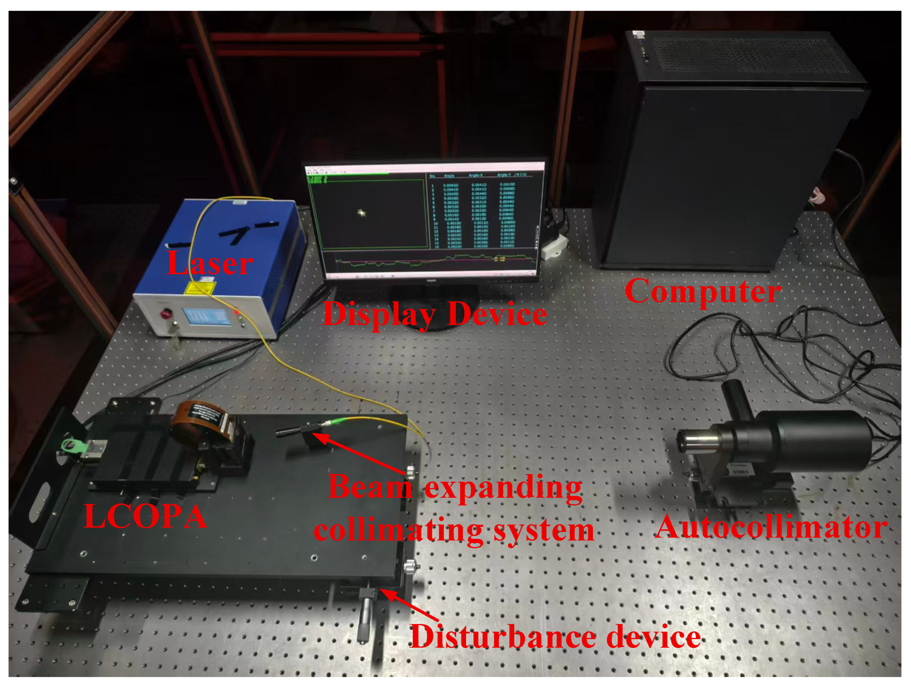
To evaluate the proposed method on an actual LCOPA beam-steering system, the platform shown in Figure 14 is constructed. It consists mainly of a laser, a beam-expansion and collimation assembly, an LCOPA, an autocollimator, a computer, and a display. The laser provides a stable input beam. The expansion and collimation assembly adjusts beam diameter and collimation and uses a linear polarizer to produce the linearly polarized light required by the LCOPA. Acting as the beam-steering actuator, the LCOPA spatially modulates the incident wavefront according to the loaded phase grayscale image and produces two-dimensional beam deflection. The autocollimator measures the actual deflection angle and sends the result to the computer over Ethernet. The computer executes the composite-control algorithm, generates steering commands, loads phase grayscale images, and acquires and processes experimental data. The display presents the control interface, target and measured angles, pointing error, and related information.

During an experiment, the computer calculates the phase distribution required for the target deflection angle and sends the corresponding grayscale image to the LCOPA. After beam expansion and collimation, the incident laser enters the LCOPA and is deflected by spatial phase modulation. The autocollimator measures the actual output-beam angle in real time and feeds it back to the computer. The computer updates the control command from the error between the target and measured angles, forming a closed-loop beam-pointing control system.

To further clarify the hardware configuration of the experimental platform and the operating conditions of the control system and to improve the reproducibility of the experimental results, the main hardware components and their key parameters are listed in

Table 9. Major equipment and parameters of the experimental platform for LCOPA beam steering.

Component	Technical Parameters
Laser	Operating wavelength: 1064 nm
Liquid crystal optical phased array	Number of array elements: 1920 × 1152; pixel pitch: 9.2 μm × 9.2 μm; maximum driving frequency: 845 Hz; operating wavelength: 600–1300 nm
Autocollimator	Angular measurement range: ±2.45° × ±2.7°; measurement accuracy: 3″; sampling frequency: 50 Hz
Computer	CPU: AMD Ryzen9 5900X (Advanced Micro Devices, Inc., Santa Clara, CA, USA); GPU: NVIDIA GeForce RTX 3070 (NVIDIA Corporation, Santa Clara, CA, USA); RAM: 64 GB
Precision adjustment stage	Adjustment range: ±10°; angular resolution: 0.01°

. The array parameters, operating wavelength, and response characteristics of the liquid crystal optical phased array determine its beam-steering capability. The collimator is used to measure the actual deflection angles along the two axes and provide closed-loop feedback, while the computer is responsible for executing the control algorithm, generating control commands, and processing the experimental data. During the experiments, the collimator acquires the actual beam deflection angles in the X- and Y-axis directions at a sampling frequency of 50 Hz, and the control program calculates the deflection errors based on each frame of feedback data and updates the control commands accordingly.

To further evaluate the real-time implementation capability of the proposed composite control method, the computational cost of the online closed-loop control process was assessed on the aforementioned computing platform. During online operation, the controller mainly performs dual-axis error calculation, fractional-order control, diagonal decoupling compensation, and Smith predictor compensation. The average computation time for a single control cycle is approximately 8 ms, with a maximum of approximately 10 ms. During online operation, the CPU utilization of the control program is approximately 3–5%, while the memory usage is approximately 100–300 MB. The autocollimator operates at a sampling frequency of 50 Hz, corresponding to a feedback sampling period of 20 ms. Since the computation time of a single control cycle is shorter than the feedback sampling period, the real-time closed-loop control requirements of the current experimental platform can be satisfied. It should be noted that both the offline parameter optimization and online closed-loop control computations in this study are performed entirely on the CPU, without GPU acceleration. The NVIDIA GeForce RTX 3070 installed on the experimental platform is not involved in the aforementioned computations.

7.2. Beam-Pointing and Decoupling Experiments

Two comparative experiments are performed, without and with the proposed composite method. Without composite control, the computer directly calculates and loads the phase grayscale image for the target angle, and the system corrects the command using autocollimator feedback. With composite control, the autocollimator measures the actual X- and Y-axis deflection angles in real time, and the computer updates the command from the error between the target and actual angles to achieve closed-loop pointing control. Both experiments use the same platform, target angles, initial state, and environmental conditions.

First, the Y-axis target is fixed at 0°, and a sequence of target angles is commanded on the X-axis. After the beam stabilizes, the autocollimator measures both actual angles; the X-axis pointing error and additional Y-axis deflection are recorded to evaluate improvements in X-axis accuracy and X-to-Y coupling. The X-axis target is then fixed at 0°, the Y-axis target is varied in the same manner, and the Y-axis main-channel error and additional X-axis deflection are measured to evaluate performance in the other steering direction.

The sampling frame rate of the autocollimator was 50 Hz. To reduce the influence of instantaneous measurement fluctuations on the experimental results, after the system output reached a steady state at each target deflection angle, 10 consecutive sets of angular data were collected and averaged to obtain the actual deflection angle for a single experimental trial. For each target deflection angle, five independent trials were conducted. The mean and standard deviation of the measured deflection angles obtained from the five independent trials were then calculated to evaluate the accuracy and repeatability of the beam-pointing control.

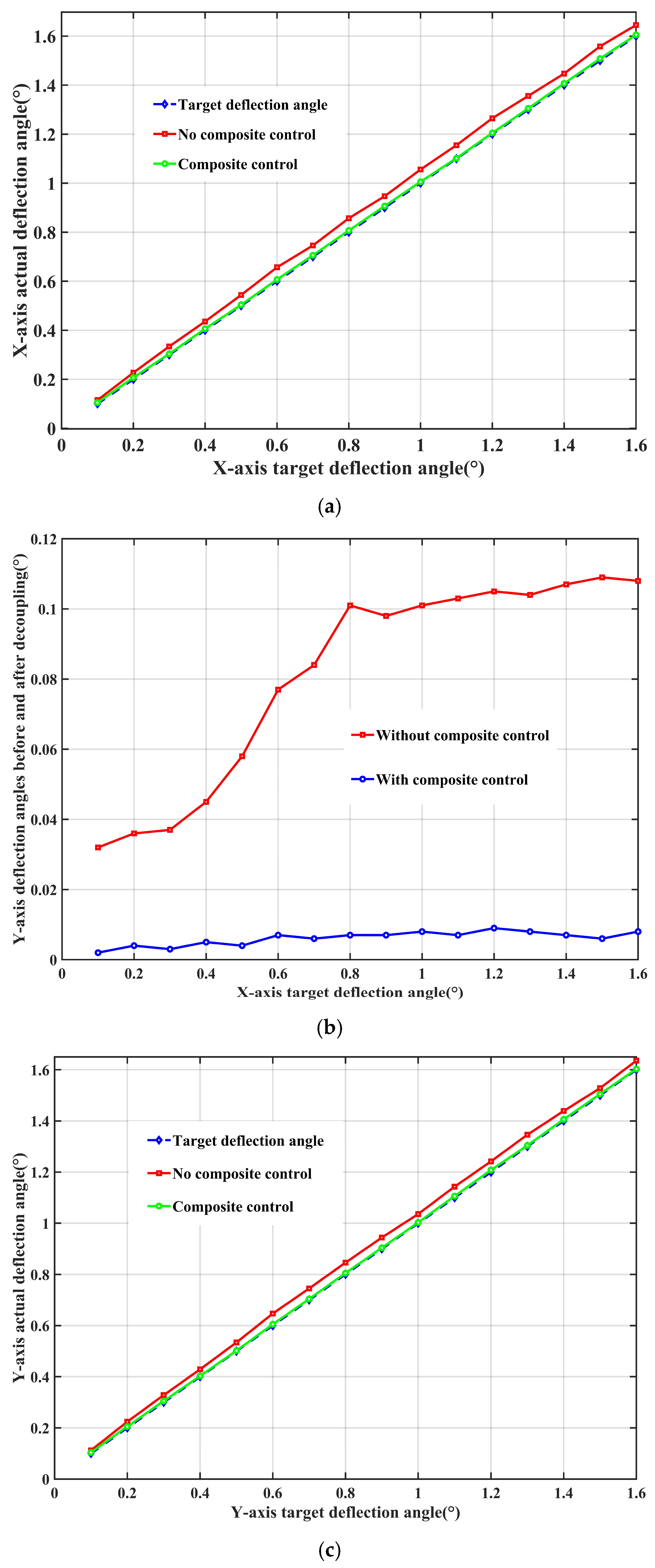
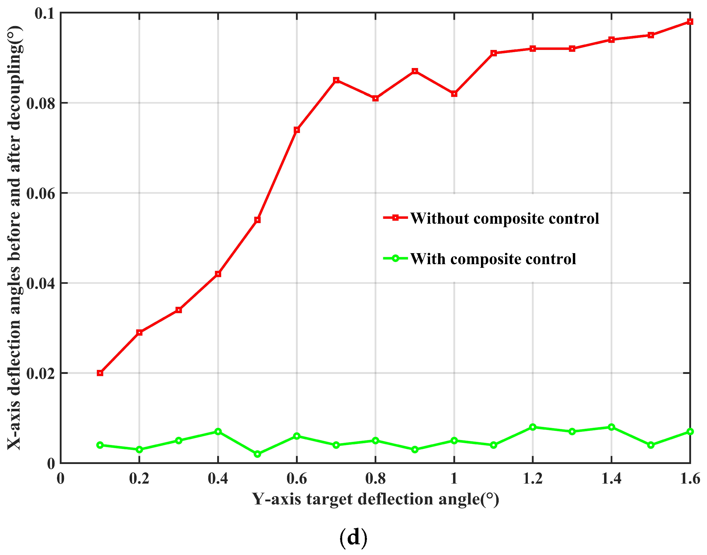
Figure 15 and

Table 10. Experimental results for two-axis decoupling control.

Steering Direction	Control Scheme	Mean Absolute Pointing Error on the Commanded Axis (°)	Mean Coupling Error (°)	Maximum Coupling Error (°)
X-axis input Y-axis held at 0°	Without composite control	0.0466	0.0816	0.1090
X-axis input Y-axis held at 0°	With composite control	0.0057	0.0061	0.0090
Y-axis input X-axis held at 0°	Without composite control	0.0362	0.0719	0.0980
Y-axis input X-axis held at 0°	With composite control	0.0045	0.0051	0.0080

show that without composite control, the measured X- and Y-axis angles deviate from their targets, and single-axis steering produces appreciable cross-coupled deflection in the other direction. With the proposed method, the mean absolute pointing errors on the X- and Y-axes decrease from 0.0466° and 0.0362° to 0.0057° and 0.0045°, respectively, demonstrating improved two-axis pointing accuracy. The mean Y-axis coupling error during X-axis steering decreases from 0.0816° to 0.0061°, while the mean X-axis coupling error during Y-axis steering decreases from 0.0719° to 0.0051°. The corresponding maximum coupling errors decrease to 0.0090° and 0.0080°, respectively. Thus, the proposed composite method improves main-channel pointing accuracy while effectively weakening coupling between the two axes.

7.3. Robustness Experiment

To verify robustness under actual external disturbances, an external disturbance-loading device is added to the platform. By changing the attitude of the optical system, the device introduces controlled angular disturbances along the beam-propagation direction, simulating pointing shifts caused by platform vibration, component installation error, and environmental disturbances.

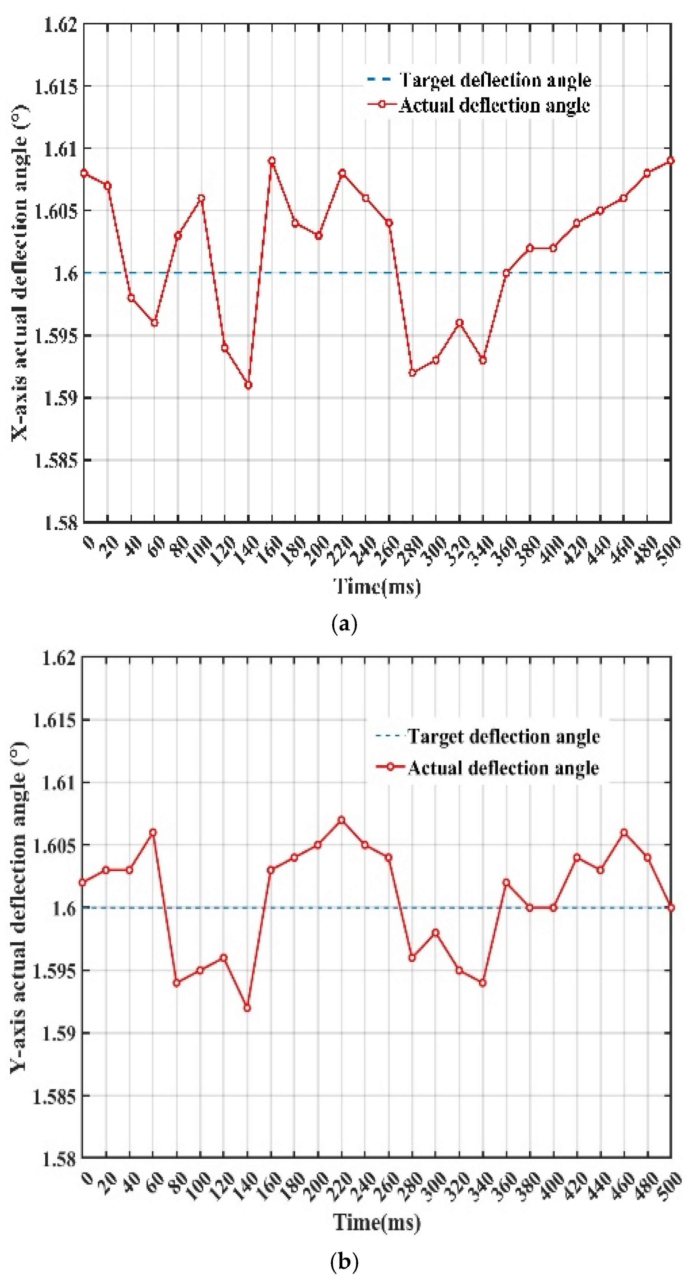
The target angle is first set, and the output was allowed to stabilize. Subsequently, angular disturbances of +0.1°and −0.1° were applied to the X- and Y-axis directions, respectively, using a precision adjustment stage with an angular scale. The disturbance amplitudes were set and controlled according to the angular scale of the precision adjustment stage to ensure consistent disturbance application under different experimental conditions. After the disturbances were applied, the autocollimator continuously measured the actual beam deflection angles at a sampling frame rate of 50 Hz and fed the measurement results back to the control system in real time. The composite controller updated the control commands in real time according to the error between the target and actual deflection angles, thereby suppressing beam-pointing deviations caused by external angular disturbances.

Figure 16 shows that under external disturbance, the measured X- and Y-axis deflection angles fluctuate only slightly around the 1.6° target, with no sustained deviation or pronounced oscillation. The root-mean-square pointing errors are 0.0060° and 0.0044° for the X- and Y-axes, respectively. The proposed composite method, therefore, effectively suppresses pointing shifts caused by external physical disturbances and holds both axis angles near their targets, providing good disturbance rejection and beam-pointing stability.

8. Conclusions

To address the time delay, channel coupling, and disturbances in liquid crystal optical phased array beam-steering systems, this paper proposes a beam-steering method based on fractional-order composite control. First, the liquid crystal optical phased array is modeled as a two-input two-output system, and a fractional-order time-delay dynamic model is established. Then, a composite control structure consisting of a fractional-order controller, a diagonal decoupling compensator, and a Smith predictor is designed. A multi-strategy fusion sparrow search algorithm is employed to optimize and tune the fractional-order controller parameters for both channels. Comparative simulations and experimental validation are conducted to evaluate the dynamic response, steady-state control accuracy, coupling suppression capability, and robustness of the proposed method.

Simulation results show that, compared with PID, FOPID, and ADRC, the proposed composite control method can further improve the dynamic response performance and steady-state control accuracy of the system. The settling times of the proposed method for both the X- and Y-axis channels are 11.50 ms, representing reductions of 62.54% and 62.30% when compared with the results for PID control, 57.09% and 56.11% compared with the results for FOPID control, and 51.68% and 48.89% compared with the results for ADRC, respectively. Meanwhile, the overshoots of the X- and Y-axis channels are 0.22% and 0.26%, respectively, while the corresponding steady-state errors are 2.38 × 10⁻³ and 2.46 × 10⁻³, both lower than those of the three comparative methods. In terms of dual-axis coupling suppression, the proposed method reduces the maximum coupling deviations from the X-axis to the Y-axis and from the Y-axis to the X-axis to 0.0036° and 0.0030°, respectively, corresponding to coupling degrees of only 0.23% and 0.19%, which are significantly lower than those achieved by PID, FOPID, and ADRC. Furthermore, under ±0.1° step disturbances, the proposed method effectively reduces the transient deviations of the beam deflection angle and enables the system to rapidly recover to the vicinity of the steady state, demonstrating good disturbance rejection capability and beam-pointing stability. In addition, to further investigate the contribution of each functional module within the composite control structure to the overall system performance, ablation simulations were conducted using different control configurations. The results show that the diagonal decoupling compensator can significantly suppress the cross-coupling between the two axes, while the Smith predictor can improve the closed-loop response characteristics in the presence of system time delay. When both modules operate in coordination with the FOPID controller, the system achieves favorable overall performance in terms of dynamic response speed, steady-state control accuracy, and coupling suppression, thereby validating the rationality of the proposed composite control structure.

The physical experiments further show that the proposed method reduces the mean absolute pointing errors on the X- and Y-axes from 0.0466° and 0.0362° to 0.0057° and 0.0045°, respectively. The mean Y-axis coupling error during X-axis steering decreases from 0.0816° to 0.0061°, and the mean X-axis coupling error during Y-axis steering decreases from 0.0719° to 0.0051°; the corresponding maximum coupling errors decrease to 0.0090° and 0.0080°, respectively. Under external physical disturbances, the X- and Y-axis root-mean-square pointing errors remain near the target at 0.0060° and 0.0044°, respectively. Overall, the proposed composite method improves LCOPA beam-pointing accuracy, weakens coupling between the two axis channels, and enhances pointing stability under external disturbances. It should be noted that the proposed method is primarily based on the coordinated design and targeted improvement of existing fractional-order control, decoupling compensation, Smith predictor compensation, and intelligent optimization methods. Its main contribution lies in the design and engineering implementation of a composite control architecture tailored to the complex dynamic characteristics of the liquid crystal optical phased array. Future work will further investigate adaptive regulation under model uncertainties to further enhance the robustness and applicability of the system.