Multiscale Fractal Feature Extraction and Identification of Fracture Images Using Complexity-Adaptive Box-Height Differential Box-Counting and SOM

Abstract

Fractures exhibit complex spatial structures and multiscale geometric characteristics, and their accurate characterization is fundamental to reservoir evaluation, fluid migration analysis, and rock mechanics. To address the limitations of single-scale local fractal methods in simultaneously capturing fracture details and global structures, as well as the dependence of supervised learning on labeled data, this study proposes an unsupervised fracture identification method integrating Complexity-Adaptive Box-Height Differential Box-Counting (CABH-DBC) with a self-organizing map (SOM). Local fractal features are extracted using fixed multiscale windows, while the box height along the gray-level dimension is adaptively refined according to the local grayscale standard deviation. The multiscale features are then fed into the SOM for clustering, with grayscale information assisting in fracture-cluster determination. Experiments on borehole image logs from ten depth intervals of the CCSD main borehole yield mean F1 and IoU values of 0.659 and 0.493, respectively. Compared with DBC-Kmeans, the proposed method improves F1 and IoU by 39.0% and 58.0%, respectively; compared with DBC-SOM, the strongest baseline in this study, the improvements are 16.6% and 24.8%. Ablation experiments further demonstrate the complementary contributions of complexity-adaptive box-height refinement, fixed multiscale fractal features, and SOM clustering.

1. Introduction

Fractures are important structural elements in complex rock masses and are widely distributed in hydrocarbon reservoirs and subsurface engineering media. Their spatial distribution, connectivity, and geometric complexity directly influence fluid migration, reservoir evaluation, and the mechanical behavior of rock masses [1,2,3]. Natural fractures are jointly controlled by multiple factors, including tectonic activity, fluid–rock interactions, and stress evolution, and therefore commonly exhibit pronounced multiscale characteristics and spatial heterogeneity [4,5,6]. Accurate characterization of fracture geometry is thus essential for fracture-network modeling, seepage analysis, and rock-mass stability assessment [7]. Borehole imaging provides continuous, high-resolution images of the borehole wall and serves as an effective data source for fracture morphology identification and quantitative analysis [8,9,10]. However, practical borehole images are often affected by complex background textures, grayscale variations, and substantial differences in fracture scale, making conventional interpretation methods that rely heavily on expert experience inadequate for large-scale quantitative fracture evaluation [11]. Moreover, effective extraction of fracture geometric characteristics requires not only the identification of fracture regions but also the characterization of their complex structural features, thereby providing reliable information for fracture-network analysis, fluid-migration simulation, and rock-mechanics studies [12,13,14,15].

Traditional geometric parameters, such as fracture length, width, and density, are insufficient to fully characterize the structural complexity of fractures. Owing to the pronounced irregularity and multiscale nature of natural fractures, fractal theory has gradually become an important mathematical tool for quantitatively describing complex fracture structures. The fractal theory introduced by Mandelbrot provides a unified framework for describing complex structures exhibiting self-similarity and scale invariance [16,17]. Fractal dimension can characterize the space-filling capacity and geometric complexity of a structure from the perspective of scale variation and has been widely applied to the analysis of fracture morphology, pore structures, and rock-surface characteristics [18,19,20]. In image analysis, Sarkar and Chaudhuri [21] proposed the differential box-counting (DBC) method, which estimates the fractal dimension of an image by counting the number of boxes required to cover its gray-level surface at different scales. The method was subsequently extended to the quantification of lacunarity in remote-sensing images [22]. Further studies improved the DBC method in terms of box-height calculation, scale-partitioning strategies, and fractal-dimension estimation accuracy [23,24], and its applications were subsequently extended to computed tomography (CT) image processing and fracture identification [25,26,27].

However, conventional DBC methods generally calculate local fractal features using a fixed-scale window, implicitly assuming that different image regions can be analyzed at the same spatial scale. This assumption is difficult to satisfy in complex fracture images containing structures at markedly different scales. When microfractures, macroscopic fractures, and complex backgrounds coexist, small-scale windows are advantageous for preserving local details but are more susceptible to noise, whereas large-scale windows provide greater stability but may cause the loss of microfracture information. Therefore, developing a fractal feature extraction method capable of accommodating variations in fracture scale while effectively balancing local details and global structural information remains a key challenge when applying DBC-based methods to complex borehole images [28].

After effective fracture features have been obtained, achieving automatic fracture identification represents another important research objective. Existing fracture identification methods mainly include conventional image-processing approaches, texture-analysis methods, and deep-learning techniques. Edge-detection- and threshold-segmentation-based methods have the advantages of simple implementation and high computational efficiency, but their performance is readily affected by noise and complex backgrounds [29]. Texture-based methods employing techniques such as the gray-level co-occurrence matrix (GLCM) and Gabor filtering can enhance the distinction between fractures and the background; however, they remain insufficiently adaptive to fracture structures exhibiting pronounced scale variations [30,31]. In recent years, deep-learning methods have achieved substantial progress in image segmentation and fracture detection because of their powerful feature-learning capabilities [32,33,34]. Nevertheless, such methods generally require large quantities of pixel-level labeled data, while fine-grained annotation of borehole images is labor-intensive and costly, thereby limiting their broader application. Consequently, combining mathematically interpretable feature descriptors with label-free learning strategies provides a promising direction for the automatic identification of fractures in complex borehole images.

The self-organizing map (SOM) is a representative unsupervised competitive-learning neural network capable of clustering high-dimensional features while preserving the topological relationships within the data, making it well suited for the analysis of complex structural data [35,36,37]. Owing to its unsupervised learning capability and topology-preserving property, SOM has been widely applied to water-resource analysis, remote-sensing image classification, and medical image processing [38,39,40]. Compared with the conventional K-means clustering algorithm [41], SOM is better able to preserve topological relationships among samples and is suitable for the analysis of nonlinear feature spaces [42].

Notably, current studies on fracture identification from borehole images still focus primarily on optimizing segmentation results. Systematic investigations into the integration of multiscale fractal features with unsupervised clustering for simultaneously characterizing fracture geometric complexity and achieving automatic fracture identification remain limited.

To address these issues, this study proposes an unsupervised fracture identification method that integrates Complexity-Adaptive Box-Height Differential Box-Counting (CABH-DBC) with a self-organizing map (SOM). The overall framework is illustrated in Figure 1.

From both methodological and practical perspectives, the main contributions of this study are twofold. First, within the DBC framework, a local grayscale-complexity-driven strategy is introduced to adaptively refine the box height, and fixed multiscale windows are employed to construct local fractal features. These features are designed to characterize the scale dependence, space-filling capacity, and geometric heterogeneity of fracture structures. Second, the multiscale fractal features are integrated with SOM-based unsupervised clustering, establishing a direct link between fractal characterization and automatic fracture identification in borehole images.

The direct mathematical foundation of this study lies in fractal geometry and fractal-dimension analysis and does not involve the formulation of fractional-order derivative or integral operators. Nevertheless, from the perspective of complex-medium modeling, the scale-dependent fractal structural information obtained in this study may provide a potential structural basis for characterizing medium heterogeneity in subsequent fractional-order transport, anomalous-diffusion, and nonlocal-flow models. The proposed method is directly intended for fracture identification in borehole images and quantitative characterization of fracture networks and may also provide supplementary information for fracture-connectivity analysis and related fluid-flow evaluation.

2. Experimental Data and Image Preprocessing

2.1. Fracture Borehole Imaging Dataset

The experimental data used in this study were obtained from borehole imaging logs acquired over the depth interval of 178–1090 m in the main hole of the Chinese Continental Scientific Drilling Project (CCSD). The data were acquired using the STAR II electrical borehole imaging system (Baker Atlas, Houston, TX, USA), with an original vertical sampling interval of 0.1 inch (approximately 2.54 mm). Experimental images were extracted interval by interval from the interpreted borehole image logs according to depth. Because the display scales of individual intervals were not completely identical, the image dimensions in pixels were not directly determined by the corresponding depth spans. Accordingly, all fractal calculations and quantitative evaluations in this study were performed in the pixel domain. The lithology within the investigated depth range is metamorphic rock. This study focuses specifically on fracture-structure identification and fractal feature extraction from borehole images and does not involve further lithological classification.

To evaluate the effectiveness of the proposed method, ten representative depth intervals within CCSD-MH (178–1090 m) were selected for quantitative experiments. These intervals contain various structural types, including microfractures, high-angle fractures, and complex fracture networks. All ten quantitative intervals were obtained from CCSD-MH and therefore represent observations from different depth intervals within a single borehole rather than mutually independent geological replicate samples. The CCSD-MH interval of 540–547 m was selected as a representative example for visualizing preprocessing and intermediate results, and the same preprocessing procedure was applied to all experimental data and all comparison methods. Information on the three representative depth intervals used in the main text for visualization of typical results and global-scale fractal analysis is summarized in

Table 1. Information on the principal representative depth intervals from CCSD-MH used in this study.

Depth Interval	Lithology	Image Size	Purpose in This Study
CCSD-MH (496–516 m)	Metamorphic rock	180 × 505 pixels	Sparse-fracture interval for global-scale fractal analysis
CCSD-MH (540–547 m)	Metamorphic rock	319 × 895 pixels	Visualization of preprocessing, multiscale features, and fracture identification
CCSD-MH (810–828 m)	Metamorphic rock	193 × 490 pixels	Dense-fracture interval for global-scale fractal analysis

.

All three representative depth intervals are located within the metamorphic-rock section investigated in this study and are used for typical visualization and analysis at different stages of the proposed workflow.

It should be noted that the same preprocessing procedure was uniformly applied to all experimental data and all comparison methods. Therefore, any effects of preprocessing on grayscale statistical characteristics are consistent across the different methods. Consequently, the reported performance differences reflect the relative performance of the methods under identical preprocessing conditions rather than absolute differences in fractal characteristics independent of the preprocessing procedure.

2.2. Image Preprocessing Procedure

Borehole images may be affected by random noise, nonuniform grayscale distributions, and insufficient local contrast. To obtain consistent input data for fractal calculations, the images were sequentially subjected to grayscale conversion, median filtering, contrast-limited adaptive histogram equalization (CLAHE), gamma correction, and final normalization.

First, the original RGB image was converted to a grayscale image:

$$I_{\mathrm{gray}}=0.299R+0.587G+0.114B,$$

(1)

where $R$, $G$ and $B$ denote the three RGB color channels, respectively, and the corresponding variable denotes the converted grayscale value [43]. The grayscale image was subsequently converted to double-precision format and mapped to the interval [0,1] [44,45]. A 3 × 3 median filter was then applied to suppress random noise [46,47]. On this basis, contrast-limited adaptive histogram equalization (CLAHE) was employed to enhance local contrast [48], followed by gamma correction to enhance details in low-grayscale regions [49,50]. After enhancement, min–max normalization was applied again so that both DBC and CABH-DBC directly operated on double-precision grayscale images with values in the range [0,1]. Therefore, the grayscale amplitude range used in the fractal calculations was [0,1], and the corresponding grayscale differences and local standard deviations were all calculated within this normalized grayscale domain.

After the above preprocessing steps, enhanced grayscale images suitable for subsequent fractal feature calculation were obtained. Taking the CCSD-MH interval of 540–547 m as an example, Figure 2 illustrates the complete image preprocessing procedure and the results obtained at each stage.

As shown in Figure 2, the sequential preprocessing steps effectively suppress noise in the original image while enhancing grayscale differences between fracture and background regions. It should be emphasized that this figure is intended solely to illustrate the preprocessing procedure and corresponds to the representative CCSD-MH interval of 540–547 m.

To intuitively illustrate the changes in grayscale distribution within the representative depth interval, Figure 3 presents the grayscale histograms before and after preprocessing.

Figure 3a shows the grayscale histogram before preprocessing, whereas Figure 3b shows the histogram after preprocessing. In both panels, the horizontal axis represents the normalized grayscale value (0–1, dimensionless), and the vertical axis represents the number of pixels falling within each grayscale interval. The notation ×10⁴ at the upper left of the vertical axis indicates the common multiplier applied to the tick values on that axis.

As shown in Figure 3, the grayscale standard deviation of the CCSD-MH (540–547 m) image increased from 0.167 before preprocessing to 0.219 after preprocessing, corresponding to an increase of approximately 31.1%. This result indicates that preprocessing broadens the grayscale distribution and improves the distinguishability between fracture and background regions, thereby providing a more stable input for subsequent fractal feature extraction.

The preprocessed borehole images obtained through the above procedure were subsequently used as the input images for multiscale fractal feature calculation and fracture identification.

3. Methodology

3.1. Differential Box-Counting Method

Differential Box-Counting (DBC) treats a two-dimensional grayscale image as a three-dimensional grayscale surface [21] and estimates its fractal dimension from the variation in the number of boxes required to cover the grayscale surface at different observation scales. For an object exhibiting fractal characteristics, the number of covering boxes $N\left(r\right)$ and the scale $r$ satisfy the following power-law relationship:

$$N(r)\propto r^{-D},$$

(2)

Taking the logarithm of both sides gives:

$$\log N(r)=-D\log r+C,$$

(3)

where $D$ denotes the fractal dimension, which quantitatively characterizes the geometric complexity of the object, and $C$ is a constant.

For a grayscale image of size $M\times M$, the pixel coordinates $\left(x,y\right)$ represent the two-dimensional spatial position, while the grayscale value $z$ is taken as the third dimension. The resulting grayscale surface can therefore be represented as:

$$I=\left(x,y,z\right),$$

(4)

At a spatial scale $s$, the image plane $\left(x,y\right)$ is partitioned into non-overlapping $s\times s$ grids, and the normalized scale is defined as:

$$r={\displaystyle \frac{s}{M}},$$

(5)

Each grid can then be regarded as being covered by a series of small boxes with dimensions $s\times s\times s$, as illustrated in Figure 4.

For the $\left(i,j\right)$-th grid, suppose that the maximum and minimum grayscale values fall into the $l$-th and $k$-th boxes, respectively, along the gray-level dimension. The number of boxes required to cover this grid is then:

$$n_r\left(i,j\right)=l-k+1,$$

(6)

Summing over all spatial grids gives:

$$N\left(r\right)={\displaystyle \sum n_r\left(i,j\right)},$$

(7)

By varying the scale $r$, a least-squares regression is performed between $\log N\left(r\right)$ and $\log \left(1/r\right)$ according to Equations (2) and (3), and the resulting slope gives the corresponding fractal dimension.

3.2. Complexity-Adaptive Box-Height Differential Box-Counting Method

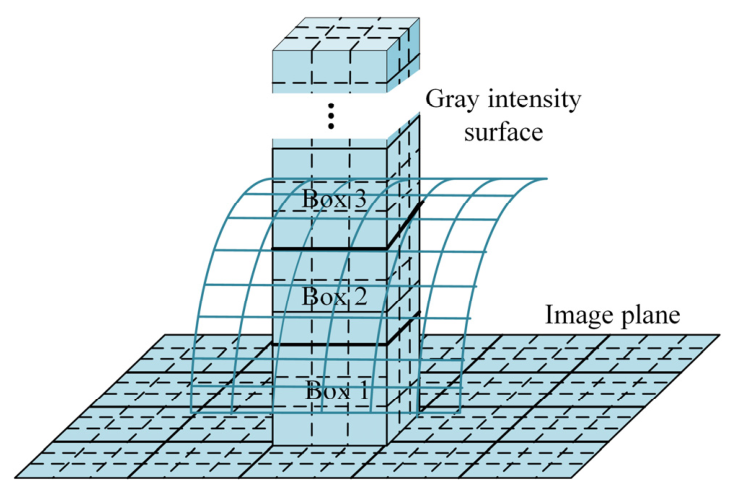
In local calculations, conventional DBC employs a fixed box height along the gray-level dimension, making it difficult to simultaneously accommodate variations in fracture scale and local grayscale complexity. In the proposed method, three analysis windows of 7 × 7, 13 × 13, and 25 × 25 pixels are evaluated at every pixel, while only the box height along the gray-level dimension is adaptively refined according to local grayscale complexity. This leads to the proposed Complexity-Adaptive Box-Height Differential Box-Counting (CABH-DBC) method.

It should be emphasized that the local complexity is not used to select, discard, or weight individual window scales on a pixel-by-pixel basis. Instead, all three windows are fully evaluated and jointly form a fixed three-dimensional feature vector.

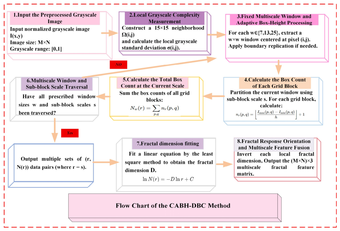
The implementation of CABH-DBC consists of four steps: (1) measurement of local grayscale complexity; (2) calculation of local fractal dimensions within multiscale windows; (3) orientation of local fractal responses; and (4) multiscale fractal feature fusion.

(1)

Local Grayscale Complexity Measurement;

Let the preprocessed grayscale image be denoted by $I\left(x,y\right)$. For an arbitrary pixel $\left(i,j\right)$, a 15 × 15 neighborhood $\mathsf{\Omega }\left(i,j\right)$ centered on that pixel is constructed. The local grayscale standard deviation is defined as:

$$\sigma \left(i,j\right)=\sqrt{{\displaystyle \frac{1}{\left|\mathsf{\Omega }\right|}}{{\displaystyle \sum _{\left(x,y\right)\in \mathsf{\Omega }\left(i,j\right)}\left[I\left(x,y\right)-\mu \left(i,j\right)\right]}}^2},$$

(8)

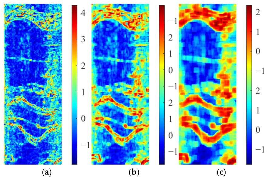
where $\mu \left(i,j\right)$ denotes the mean grayscale value within the neighborhood and $\left|\mathsf{\Omega }\right|=225$. Because the input grayscale values have been normalized to [0,1], $\sigma \left(i,j\right)$ is dimensionless and satisfies $0\le \sigma \left(i,j\right)\le 0.5$. The value of $\sigma \left(i,j\right)$ reflects the magnitude of local textural variation. Homogeneous regions generally exhibit relatively small values, whereas structurally varying regions, such as fracture edges, pore boundaries, and texture interfaces, tend to exhibit larger values.

It is important to distinguish the spatial meanings of these responses. High values of $\sigma$ occur predominantly within transition zones between fractures and the surrounding background, whereas the low local fractal-dimension values discussed below primarily occur within the interior of the dark fracture bands. Thus, the two quantities characterize different parts of the fracture structure.

(2)

Local Fractal-Dimension Calculation within Multiscale Windows;

Let the set of analysis-window sizes be $W=\left\{7,13,25\right\}$. For each scale $w\in W$ and each pixel $\left(i,j\right)$, a $w\times w$ analysis window $W_w\left(i,j\right)$ centered at that pixel is constructed. When the window extends beyond the image boundary, the out-of-bound region is padded by replicating the nearest boundary pixel values.

Within each analysis window, the sub-block scale s is varied. To adjust the quantization resolution along the gray-level dimension according to local grayscale complexity, the adaptive box height is defined as:

$$h={\displaystyle \frac{s/w}{1+2a\sigma (i,j)}},$$

(9)

where $s/w$ is the dimensionless normalized spatial scale, $\sigma \left(i,j\right)$ is the dimensionless local grayscale standard deviation, and $a$ is also a dimensionless parameter. Therefore, $h$ represents the box height within the normalized grayscale domain and is expressed on the same normalized scale as the grayscale range used in the equation.

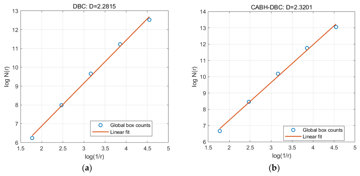
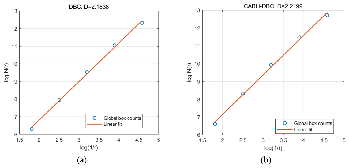
Because the actual differential box-counting procedure involves discrete rounding operations, variations in box height may alter the number of covering boxes at different scales and consequently change the estimated fractal dimension. Therefore, the proposed method does not assume a priori that adaptive box-height refinement necessarily improves fitting linearity or preserves the numerical value of the fractal dimension.

For each grid block within the window, the number of boxes required for coverage is calculated as:

$$n_r\left(i,j\right)=⌊{\displaystyle \frac{I_{\max }\left(i,j\right)-I_{\min }\left(i,j\right)}{h}}⌋+1,$$

(10)

where $I_{\max }$ and $I_{\min }$ are the maximum and minimum grayscale values within the corresponding grid block, respectively. The term +1 ensures that one box is still counted when the two extreme grayscale values fall within the same box.

Summing over all grid blocks within the analysis window yields

$$N_r={\displaystyle \sum _{i,j}{n}_r\left(i,j\right)},$$

(11)

The sub-block scale $s$ is varied within each window according to $s\in \{1,\dots ,⌊w/2⌋\}$. When more than six candidate scales are available, six scales are selected with logarithmically uniform spacing. The spatial scale is normalized as $r=s/w$. Taking logarithms of the power-law relationship in Equation (2) gives Equation (3). Least-squares fitting in log-log coordinates then yields the local fractal dimension $D_w\left(i,j\right)$ at pixel $\left(i,j\right)$ for window size $w$.

By traversing the entire image and performing the calculation separately at the three window scales, three local fractal-dimension feature maps are obtained $D_7\left(i,j\right)$, $D_{13}\left(i,j\right)$ and $D_{25}\left(i,j\right)$.

(3)

Orientation of Local Fractal Responses;

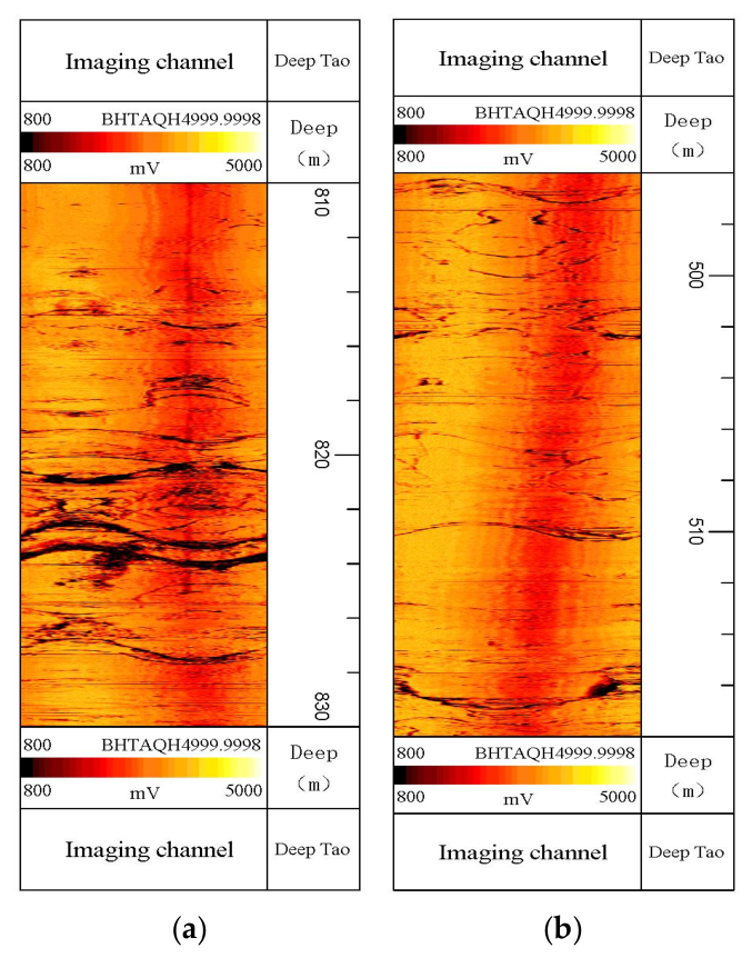
DBC estimates the local box dimension of a grayscale surface. For a locally self-affine grayscale surface, the local roughness can be described by $D=3-H$, where $H$ is the Hurst exponent. In the data analyzed in this study, fractures predominantly appear as continuous low-resistivity dark bands in the enhanced borehole images. Grayscale variations within these bands are relatively smooth, and their local fractal dimensions therefore tend to lie toward the lower end of the distribution for a given image. In contrast, background regions with more complex textures generally exhibit higher local fractal dimensions.

To ensure that larger responses consistently correspond to fractures in the subsequent classification procedure, the local fractal dimension at each scale is linearly inverted:

$$D_{w,inv}(i,j)=D_{w,\min }+D_{w,\max }-D_w(i,j),$$

(12)

where $D_{w,\min }$ and $D_{w,\max }$ are the minimum and maximum local fractal dimensions, respectively, for the image at scale $w$.

This operation is an affine transformation with a slope of -1 and preserves the absolute difference in fractal dimension between any two pixels. After Z-score standardization of the feature matrix, the transformation is exactly equivalent to negating the standardized feature and therefore constitutes an isometric transformation in Euclidean space. Consequently, the partitions obtained by K-means and SOM based on Euclidean distance are unaffected by this transformation; only the assignment of which cluster is interpreted as the fracture cluster is changed.

The inversion itself introduces no additional discriminative information, and the features supplied to the SOM remain entirely derived from the local fractal dimensions. Grayscale information is introduced only as auxiliary information for the semantic determination of the final fracture clusters, as described in Section 3.3.

The above criterion requires an analysis window to contain both a fracture and its adjacent background. When the fracture width exceeds the size of a small analysis window, the interior of the window may again become relatively homogeneous. The use of three fixed window sizes allows the larger windows to retain the possibility of spanning the boundary between a fracture and its neighboring background, thereby preserving structural information at different spatial scales.

Following response orientation, three local fractal response maps $D_{w,inv}(i,j)$ are obtained for subsequent multiscale feature fusion. It should be noted that the full-interval fitting performed in Section 4.1.1 directly uses the original $D$ values without inversion.

(4)

Multiscale Feature Fusion.

For each pixel $\left(i,j\right)$, the local fractal responses at the three scales are stacked to form a three-dimensional feature vector:

$$d\left(i,j\right)={\left[D_{7,inv}\left(i,j\right),D_{13,inv}\left(i,j\right),D_{25,inv}\left(i,j\right)\right]}^T,$$

(13)

The entire image therefore produces a fractal feature matrix of size $\left(M\times N\right)\times 3$, which serves as the input to the SOM described in Section 3.3. All three scales are fully retained. No specific window scale is assumed a priori to dominate a particular complexity regime; instead, the subsequent SOM organizes the feature space according to the joint distribution of the three-dimensional fractal responses.

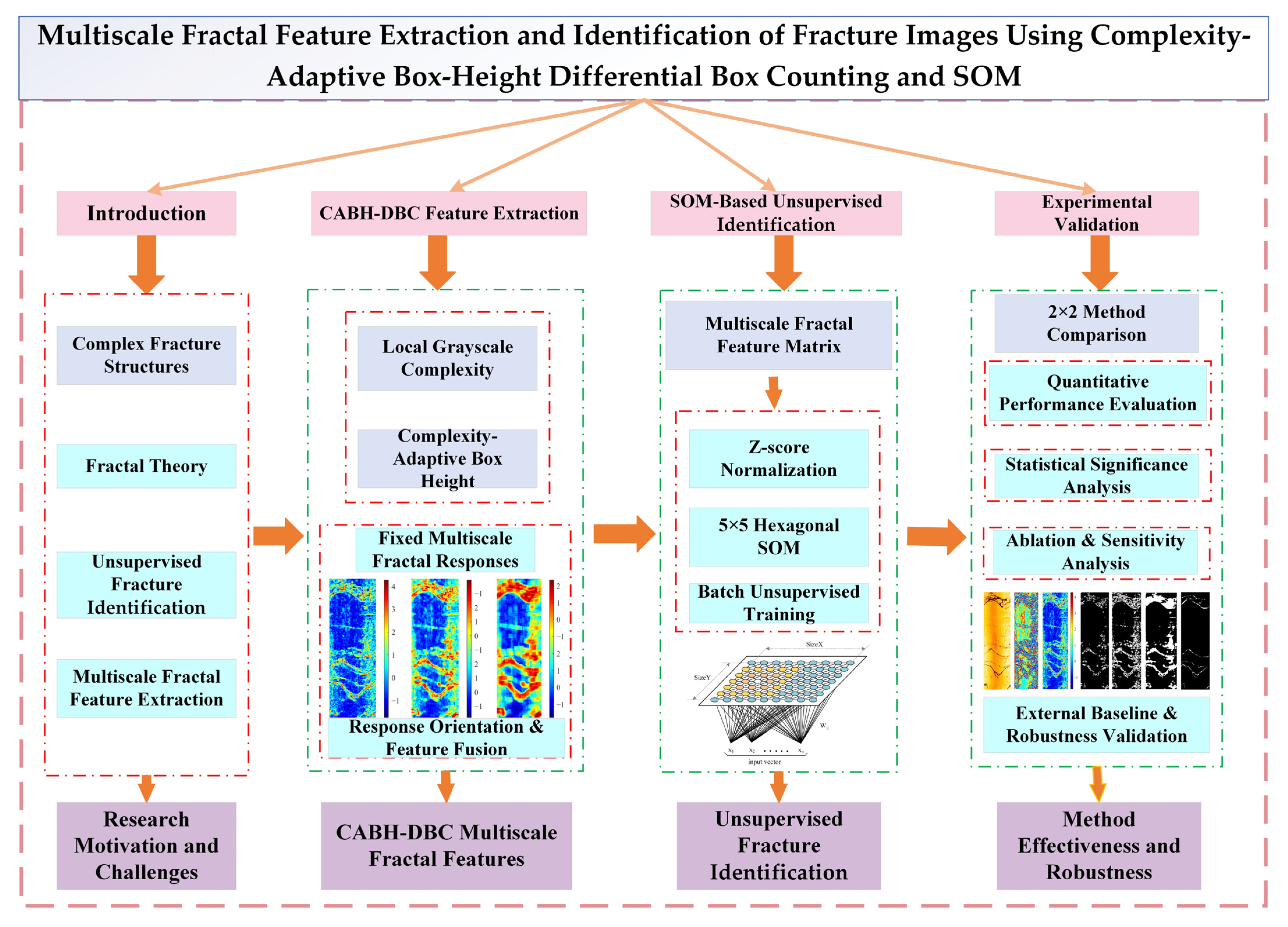
Figure 5 illustrates the overall workflow of the CABH-DBC algorithm. Through the above procedure, the inverted local fractal response maps are obtained and subsequently used as SOM input features for fracture identification.

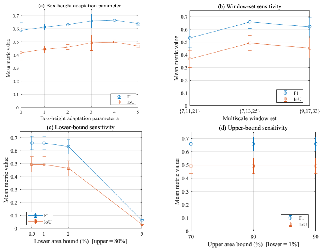
In this study, a 15 × 15 neighborhood for local complexity estimation and multiscale windows of $\left\{7,13,25\right\}$ are fixed throughout the main experiments. The box-height adaptation parameter was fixed a priori at $a=3$ before the quantitative evaluation and was kept unchanged throughout the main experiments. The 15 × 15 neighborhood provides a balance between the stability of standard-deviation estimation and spatial locality. The three windows, which approximately follow a doubling progression, cover local structural scales ranging from several pixels to several tens of pixels and are designed to accommodate both narrow and relatively wide fractures in the pixel domain.

The parameter $a$ controls the degree of box-height refinement. An excessively small $a$ weakens the effect of complexity adaptation, whereas an excessively large value may increase sensitivity to local noise. The corresponding sensitivity analysis is presented in Section 4.4.2.

3.3. Self-Organizing Map

The self-organizing map maps high-dimensional features onto a low-dimensional topological grid through competitive learning and neighborhood updating. For an input feature vector $x_i$, let $w_j$ denote the weight vector of the $j$-th neuron. The best matching unit (BMU) is defined as:

$$c=\arg \min ‖x-w_j‖,$$

(14)

where $c$ denotes the index of the winning neuron.

After the BMUs of all samples have been determined, the network weights are updated in batch mode. The neighborhood-weighted sample mean for the $j$-th neuron is given by:

$$m_j(t)={\displaystyle \frac{{\displaystyle \sum _i{\varphi }_{j,c(i)}}(t)x_i}{{\displaystyle \sum _i{\varphi }_{j,c(i)}}(t)}} ,$$

(15)

and the weight vector is updated as:

$$w_j(t+1)=[1-\eta (t)]w_j(t)+\eta (t)m_j(t),$$

(16)

where the neighborhood function is defined as:

$${\varphi }_{j,c}(t)=\exp \left[-{\displaystyle \frac{d^2(j,c)}{2{\rho }^2(t)}}\right],$$

(17)

here, $d\left(j,c\right)$ denotes the link distance between neurons $j$ and $c$ on the hexagonal grid, $\rho \left(t\right)$ is the neighborhood radius, and $\eta \left(t\right)$ is the learning rate.

Equation (16) performs a convex combination based on the batch neighborhood-weighted mean, with the combination controlled by $\eta \left(t\right)$. Feature standardization, clustering, and fracture-cluster determination are all performed independently for each image, and no parameters are shared across different depth intervals.

Before the three-dimensional CABH-DBC feature vectors are supplied to the SOM, each feature dimension is standardized using Z-score normalization to eliminate scale differences among feature dimensions:

$$X_k^{\prime }={\displaystyle \frac{X_k-{\mu }_k}{{\sigma }_k}},$$

(18)

where ${\mu }_k$ and ${\sigma }_k$ denote the mean and standard deviation of the $k$-th fractal feature dimension, respectively.

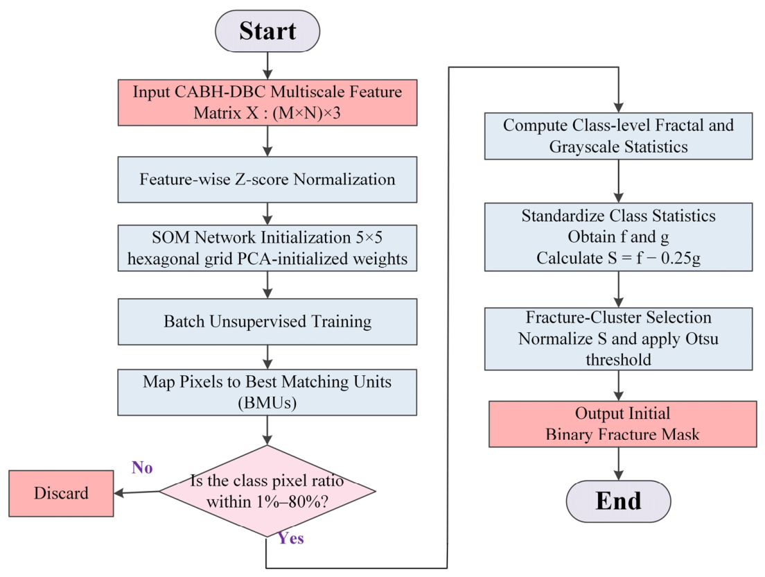
To obtain stable clustering results, a 5 × 5 hexagonal SOM is employed. The weights are initialized using principal components, followed by batch unsupervised training for 200 epochs. The neighborhood radius is geometrically decayed from 3 to 0.5, while the learning rate is geometrically decayed from 0.5 to 0.05.

After training, three statistics are calculated for each neuron-defined class: the proportion of pixels assigned to the class, the mean response of those pixels across the three Z-score-normalized feature dimensions, and the mean grayscale value of the corresponding pixels in the pre-enhancement grayscale image. Only classes with pixel proportions between 1% and 80% are retained, thereby excluding noise classes with excessively small areas and background classes with excessively large areas. This area-based screening range is fixed in the main experiments, and its sensitivity is evaluated in Section 4.4.2.

For the retained classes, the latter two quantities are separately Z-score standardized across classes and denoted by $f$ and $g$, respectively. A fracture-cluster score is then constructed as $S=f-0.25g$. Since $f$ and $g$ are separately standardized, the coefficient 0.25 serves as a relative weighting factor. It was empirically set a priori and was not tuned using the ten evaluation intervals. The relatively small value was intended to keep the fractal response as the primary criterion while retaining grayscale information only as an auxiliary term for semantic fracture-cluster determination. After normalization of the scores, Otsu’s thresholding method [51] is applied to distinguish candidate fracture classes from background classes. 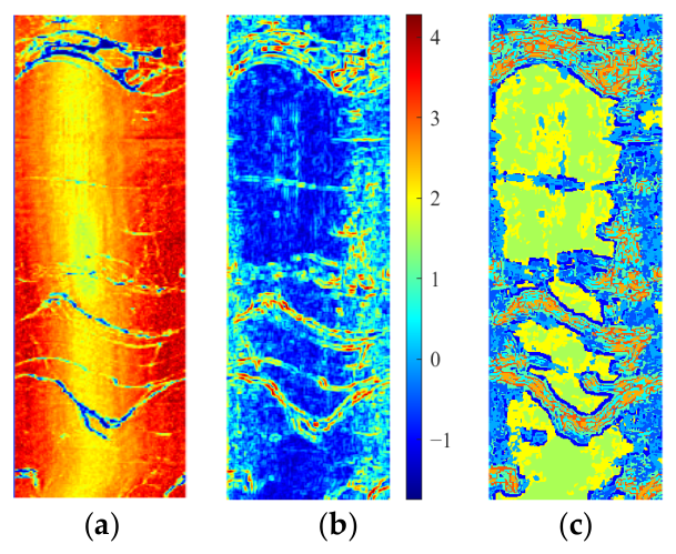Candidate classes are then accumulated in descending order of $S$, subject to the constraint that the total area proportion of the finally selected classes does not exceed 80%. Because the features at each scale have already undergone linear inversion, no additional grayscale inversion is performed at this stage, as illustrated in Figure 6.

In this study, the SOM is used to organize and partition the fractal feature space constructed by CABH-DBC rather than to replace the fractal feature extraction process. Through unsupervised topological mapping, it establishes an effective link between fractal characterization and automatic fracture identification.

4. Experimental Results and Analysis

4.1. Results and Analysis of CABH-DBC Multiscale Fractal Feature Extraction

4.1.1. Comparative Analysis of Global-Scale Fractal Dimensions

To investigate the influence of complexity-adaptive box height on the global fractal characterization of fracture images, two representative depth intervals exhibiting different degrees of fracture development were selected for comparative analysis. CCSD-MH (810–828 m) represents a relatively fracture-dense interval, whereas CCSD-MH (496–516 m) represents a relatively fracture-sparse interval, as shown in Figure 7.

Because CABH-DBC modifies the definition of the box height along the gray-level dimension, the absolute fractal-dimension values obtained using CABH-DBC should not be regarded as numerically equivalent to literature results obtained using the conventional DBC box-height definition. Therefore, this section focuses only on the relative characterization differences between the two box-height strategies under identical data and spatial-scale conditions.

This global analysis is independent of the pixel-wise local fractal feature calculation used for fracture identification in Section 3.2. Its purpose is to verify that, at the whole-image scale, the modified box-height strategy preserves the relative relationship whereby the fracture-dense interval exhibits a higher fractal dimension than the fracture-sparse interval; in other words, the modification does not destroy the monotonic relationship of the fractal characterization.

Let the size of the preprocessed image be $M\times N$, and define $L=\min \left(M,N\right)$ as the reference length. For the whole image, spatial box sizes increasing in powers of two are adopted: $q\in \left\{2,4,\dots ,2^K\right\}$, where the maximum scale satisfies $2^K\le L/4$ and the normalized scale is defined as $r=q/L$. For conventional DBC, a uniform box height along the gray-level dimension is used at scale $q$: $h_{DBC}=q/L$.

For global CABH-DBC, the local standard-deviation map $\sigma \left(x,y\right)$ is first calculated according to Section 3.2. For each spatial grid, the standard deviation at its center, ${\sigma }_{u,v}$, is taken as the representative local complexity, and the corresponding adaptive box height is defined as $h_{CABH}\left(q,u,v\right)={\displaystyle \frac{q/L}{1+2a{\sigma }_{u,v}}}$. The total number of covering boxes $N\left(r\right)$ over the entire image is then calculated at each scale, and linear fitting is performed according to $\log N\left(r\right)=D_{pool}\log \left(1/r\right)+C$ where the fitted slope $D_{pool}$ is taken as the global fractal dimension of the image.

The results are shown in Figure 8 and Figure 9.

As shown in Figure 8 and Figure 9, for the fracture-dense CCSD-MH interval of 810–828 m, the global fractal dimensions obtained using DBC and CABH-DBC are 2.2815 and 2.3201, respectively. For the relatively fracture-sparse CCSD-MH interval of 496–516 m, the corresponding values are 2.1838 and 2.2199. Both methods preserve the relative relationship in which the fracture-dense interval has a higher fractal dimension than the fracture-sparse interval.

Compared with conventional DBC, CABH-DBC increases the fractal dimensions of the two representative intervals by 0.0386 and 0.0361, respectively. This indicates that local-complexity-driven box-height adaptation alters the box-counting results at different spatial scales and consequently produces a modest numerical change in the estimated fractal dimension. This global-scale analysis is used only to compare the two box-height strategies; subsequent fracture identification continues to employ the three fixed local windows defined in Section 3.2.

4.1.2. Visualization of Multiscale Fractal Features

To further investigate the ability of the multiscale fractal features extracted by CABH-DBC to characterize fracture structures, local fractal dimensions were calculated for the CCSD-MH (540–547 m) borehole image using three window sizes, namely 7 × 7, 13 × 13, and 25 × 25. The corresponding response maps were then generated after orientation according to Equation (12).

As shown in Figure 10, the oriented local fractal responses at different scales exhibit clear scale complementarity, with high response values corresponding to the low-value end of the original local fractal-dimension distribution. The small-scale window preserves fine-scale fracture details; the intermediate-scale window provides a balance between local details and structural continuity; and the large-scale window emphasizes the overall spatial distribution of the fracture structures.

It should be noted that Figure 10 displays the inverted responses after Z-score standardization. The values on the color bars are dimensionless standardized quantities and may therefore be negative; they do not represent the original local fractal-dimension values.

Moreover, the global fractal dimension in Section 4.1.1 and the pixel-wise local fractal dimensions considered here correspond to different observation levels. The former characterizes the overall roughness of the grayscale surface of the entire image, whereas the latter is used to localize fracture-related responses. At the global scale, fractures introduce cross-scale structures and boundaries that increase the value of $D$ for the entire grayscale surface. Within a local window, however, the interior of a dark fracture band may exhibit relatively smooth grayscale variation, resulting in a lower local $D$. Therefore, the numerical trends of the global and local fractal dimensions are not required to be consistent.

Together, the three scale-dependent features constitute a multiscale fractal description space, allowing fracture structural information at different spatial scales to be jointly represented and providing a richer feature basis for subsequent SOM-based unsupervised clustering.

4.2. Visualization of SOM-Based Fracture Clustering and Segmentation

Based on the multiscale fractal features obtained in Section 4.1, SOM is further employed to perform unsupervised clustering of fracture-related feature patterns and generate the corresponding fracture identification results. The representative CCSD-MH (540–547 m) interval is selected for visualization, as shown in Figure 11.

During SOM clustering, pixels are organized according to their multiscale fractal features, enabling the spatial–structural differences in fracture regions to be represented and thereby improving the distinguishability between fracture and non-fracture regions in complex backgrounds.

To further improve the continuity of the binary result, a fixed morphological post-processing procedure is applied. First, a closing operation is performed using a disk-shaped structuring element with a radius of 1 pixel, followed by an opening operation using the same structuring element. Finally, 8-connected-component analysis is used to remove connected regions with areas smaller than 50 pixels. The resulting image is taken as the final binary mask for subsequent quantitative evaluation.

4.3. Comprehensive Comparative Analysis of Fracture Identification Performance

4.3.1. Experimental Design and Evaluation Metrics

To comprehensively evaluate the effectiveness of the proposed CABH-DBC-SOM method for fracture identification, ten representative depth intervals within the CCSD-MH depth range of 178–1090 m were selected for quantitative comparison.

All test images were processed using the preprocessing procedure described in Section 2.2. The ground-truth annotations used for quantitative evaluation were independently produced by two annotators. Based on continuous dark, low-resistivity bands in the images, together with fracture orientation and propagation direction, both annotators independently delineated fractures at the pixel level for all ten test intervals.

Before cross-review and consensus correction, the mean IoU between the two independent fracture masks was 0.848. The two annotators subsequently cross-reviewed the regions of disagreement and revised the annotations through consensus to generate the final ground truth.

To separately investigate the effects of the fractal feature extraction strategy and clustering method on fracture identification, a two-dimensional feature extraction method × clustering strategy experimental framework was constructed, comprising four combinations:

(1)

DBC-Kmeans: Conventional DBC with a fixed window is used to extract fractal features, followed by K-means clustering and segmentation. This combination serves as the baseline method.

(2)

DBC-SOM: DBC is retained for feature extraction, while K-means is replaced by SOM. This configuration is designed to isolate the effect of SOM relative to K-means under the same DBC feature representation.

(3)

CABH-DBC-Kmeans: The proposed CABH-DBC method is used for feature extraction, while K-means is retained as the clustering algorithm. This configuration is designed to evaluate, under a fixed K-means clustering strategy, the combined contribution of complexity-adaptive box height and fixed multiscale feature construction relative to conventional DBC.

(4)

CABH-DBC-SOM: CABH-DBC is used to extract multiscale fractal features, followed by SOM-based unsupervised clustering and segmentation. This configuration represents the complete proposed method.

This 2 × 2 experimental design makes it possible to separately evaluate the contributions of the CABH-DBC and SOM modules and to examine whether their combination provides complementary benefits.

For both DBC-Kmeans and CABH-DBC-Kmeans, the number of clusters is set to $k=2$, consistent with the binary fracture/non-fracture classification task considered in this study. To ensure consistency in the comparison between clustering methods, the K-means results employ the same class-area screening, combined fractal–grayscale scoring, and threshold-based decision rules described in Section 3.3.

The remaining major parameter settings are as follows: DBC uses a 13 × 13 window with a maximum of six sub-block scales per window; CLAHE uses 8 × 8 tiles and a clip limit of 0.02; the gamma exponent is set to 0.6; and K-means uses k-means++ initialization with five repetitions. Random seeds are deterministically specified for each image and method to ensure reproducibility.

Because fracture pixels generally occupy only a small fraction of a borehole image, the fracture identification task exhibits pronounced class imbalance. Therefore, Precision, Recall, F1-score, Intersection over Union (IoU), False Positive Rate (FPR), and False Negative Rate (FNR) are adopted as evaluation metrics.

F1 and IoU measure the agreement between predicted fractures and manually annotated ground truth. Precision and FPR characterize the ability to control false identifications, whereas Recall and FNR reflect the completeness of fracture-region extraction. Together, these complementary metrics enable a more comprehensive assessment of fracture identification performance in complex borehole images.

4.3.2. Visualization of Fracture Identification Results

Figure 12 presents the segmentation results obtained using the four methods for the representative CCSD-MH (540–547 m) interval.

As shown in Figure 12, the four methods exhibit different identification characteristics. DBC-Kmeans can identify some of the major fracture structures; however, because fixed-scale fractal features and conventional clustering have limited ability to distinguish complex backgrounds, a relatively large number of non-fracture regions are incorrectly identified as fractures.

When the DBC features are kept unchanged and SOM clustering is introduced, the DBC-SOM results become more spatially concentrated, and some background noise is suppressed, indicating that topology-preserving clustering can improve the partitioning of the feature space. Nevertheless, because the input features are still derived from fixed-scale DBC, their capacity to represent complex fracture structures remains limited, and discontinuities remain along some fracture boundaries.

After replacing DBC features with CABH-DBC features, CABH-DBC-Kmeans further reduces false identification of background regions and makes the principal fracture structures more prominent, indicating that the multiscale fractal features improve the distinguishability between fractures and the background. However, because K-means partitions the feature space primarily according to distance, it remains limited when handling fracture features with complex distributions, and the continuity of some local fractures can still be improved.

In comparison, CABH-DBC-SOM combines multiscale fractal feature extraction with topology-preserving clustering and exhibits better overall performance in terms of fracture structural integrity, boundary continuity, and background suppression. These observations indicate that CABH-DBC improves fracture feature representation, while SOM further improves the organization of the fractal feature space; their combination therefore produces more stable fracture identification results.

It should be noted that Figure 12 shows the result for only one representative CCSD-MH (540–547 m) depth interval, whereas

Table 2. Comprehensive performance comparison of different fracture identification methods.

Method	Precision	Recall	F1	IoU	FPR	FNR
DBC-Kmeans	0.403 ± 0.094	0.609 ± 0.093	0.474 ± 0.046	0.312 ± 0.040	0.0695 ± 0.0359	0.391 ± 0.093
DBC-SOM	0.534 ± 0.109	0.634 ± 0.097	0.565 ± 0.032	0.395 ± 0.031	0.0416 ± 0.0273	0.366 ± 0.097
CABH-DBC-Kmeans	0.486 ± 0.082	0.667 ± 0.088	0.554 ± 0.051	0.384 ± 0.049	0.0505 ± 0.0264	0.333 ± 0.088
CABH-DBC-SOM	0.633 ± 0.089	0.697 ± 0.065	0.659 ± 0.053	0.493 ± 0.060	0.0295 ± 0.0134	0.303 ± 0.065

reports the average performance over all ten test intervals. In addition, Recall depends on the pixel-wise overlap between the predicted fracture regions and the manually annotated ground truth rather than on the total area of the predicted fracture regions. Consequently, there is no simple one-to-one relationship between the apparent sparsity of the visual results and the mean Recall values reported in Table 2.

4.3.3. Quantitative Performance Evaluation

The quantitative results obtained by the four methods over the ten depth intervals are summarized in Table 2.

The four methods exhibit clear differences across the evaluation metrics. CABH-DBC-SOM achieves a mean F1-score of 0.659 and a mean IoU of 0.493. Relative to DBC-Kmeans, these values correspond to improvements of approximately 39.0% and 58.0%, respectively. Compared with DBC-SOM, the strongest-performing internal baseline, the corresponding improvements are approximately 16.6% and 24.8%.

Further comparison of the different module combinations shows that, when the clustering method is held constant, CABH-DBC provides better fracture identification performance than conventional DBC, indicating that the multiscale fractal feature extraction strategy provides a more effective representation of fracture structures. Conversely, when the feature extraction strategy is held constant, SOM outperforms K-means, indicating that topology-preserving clustering is more suitable for organizing and partitioning complex fractal feature spaces.

A Friedman test [52] was conducted to compare the F1-scores of the four methods over the ten depth intervals. The result was ${\chi }^2=20.4$, $p=1.4\times {10}^{-4}$.

As shown by the boxplots in Figure 13, the overall F1 distribution of CABH-DBC-SOM is shifted upward and exhibits the highest median, consistent with the statistically significant Friedman-test result.

Pairwise comparisons were subsequently conducted using the Wilcoxon signed-rank test [53], with Holm correction [54] applied for multiple comparisons. The results are presented in

Table 3. Pairwise significance tests of F1-scores among the different methods.

Comparison (A vs. B)	Mean Difference (A−B)	Wilcoxon $\mathit{p}$	Holm-Adjusted $\mathit{p}$	Significance
CABH-DBC-SOM vs. DBC-Kmeans	+0.185	0.0020	0.012	*
CABH-DBC-SOM vs. DBC-SOM	+0.094	0.0039	0.020	*
CABH-DBC-SOM vs. CABH-DBC-Kmeans	+0.105	0.0039	0.020	*
DBC-SOM vs. DBC-Kmeans	+0.091	0.0059	0.020	*
CABH-DBC-Kmeans vs. DBC-Kmeans	+0.080	0.0098	0.020	*
DBC-SOM vs. CABH-DBC-Kmeans	+0.012	0.557	0.557	ns

Note: The significance level is $\alpha =0.05$; * indicates $p<0.05$, and ns indicates a non-significant difference.

.

Within the ten depth intervals selected from the single CCSD-MH borehole, CABH-DBC-SOM achieves statistical significance relative to each of the other three methods after Holm correction. No significant difference is observed between DBC-SOM and CABH-DBC-Kmeans, with both methods exhibiting intermediate performance.

From a statistical perspective, this indicates that introducing SOM into conventional DBC and introducing complexity-adaptive box height together with fixed multiscale features into K-means provide gains of comparable magnitude. The best performance is obtained only when the two components are combined, consistent with the results in Table 2.

Furthermore, for a sample size of $n=10$, the minimum attainable two-sided $p$-value of the Wilcoxon signed-rank test is approximately 0.002. Therefore, the smallest $p$-value reported in Table 3 should be interpreted as the lower limit of the test resolution for the present sample size.

To examine relative performance across individual depth intervals, Figure 14 compares the F1-scores of the four methods over the ten test intervals.

Within the ten depth intervals selected from the single CCSD-MH borehole, the F1-scores of CABH-DBC-SOM indicate that its relative performance advantage is consistent across the tested intervals of this borehole. This conclusion is restricted to the current single-borehole sample and should not be interpreted as evidence of independent geological replication or cross-well generalization.

4.3.4. Ablation Study

Based on the 2 × 2 combination results reported in Table 2, the relative changes associated with the CABH-DBC feature extraction module and the SOM clustering module are averaged over the two levels of the other factor, yielding the results shown in

Table 4. Contributions of the CABH-DBC feature extraction module and SOM clustering module.

Factor	Mean Relative Improvement in F1	Mean Relative Improvement in IoU	Mean Reduction in FPR	Mean Reduction in FNR
CABH-DBC feature extraction module	≈16.8%	≈24.0%	≈28.2%	≈16.0%
SOM clustering module	≈19.1%	≈27.5%	≈40.9%	≈7.7%

. This table is intended to describe module contributions and does not constitute a formal statistical test of interaction effects.

CABH-DBC primarily improves the representation of multiscale fracture structures and reduces missed detections, whereas SOM produces a more pronounced improvement in feature-space organization and false-positive control. The two modules therefore contribute in different ways and exhibit complementary effects in the complete method.

It should be noted that the overall gain attributed to the CABH-DBC feature extraction module in Table 4 includes the combined effects of fixed multiscale feature construction and complexity-adaptive box height. These two effects are not separately isolated by the 2 × 2 experiment. The contribution of box-height adaptation alone is further evaluated in Section 4.4.2.

Overall, the ablation results verify that both core modules proposed in this study make independent contributions and further demonstrate that the combination of multiscale fractal feature extraction and topology-preserving unsupervised clustering is a key factor in improving fracture identification performance in complex borehole images.

4.4. Supplementary Validation and Sensitivity Analysis

4.4.1. Ablation Study of the Grayscale Auxiliary Term

To evaluate the influence of the grayscale auxiliary term in the fracture-cluster scoring function described in Section 3.3, the CABH-DBC features, SOM network, class-area screening, and morphological post-processing are all kept unchanged, while the scoring function of the complete method, $S=f-0.25g$, is replaced with $S=f$. This configuration forms the Fractal-only control, in which only the fractal response is used. The results are presented in

Table 5. Ablation results for the grayscale auxiliary term.

Method	Precision	Recall	F1	IoU	FPR	FNR
Fractal-only $(S=f$)	0.606 ± 0.110	0.658 ± 0.076	0.626 ± 0.078	0.460 ± 0.084	0.0312 ± 0.0148	0.342 ± 0.076
Full ($S=f-0.25g$)	0.633 ± 0.089	0.697 ± 0.065	0.659 ± 0.053	0.493 ± 0.060	0.0295 ± 0.0134	0.303 ± 0.065

.

Using only the fractal response still yields a mean F1-score of 0.626 and a mean IoU of 0.460, indicating that the CABH-DBC fractal features themselves possess substantial discriminative capability for fractures. After incorporating the grayscale auxiliary term, F1 and IoU increase to 0.659 and 0.493, respectively, while FNR decreases from 0.342 to 0.303. A paired Wilcoxon signed-rank test on the F1-scores across the ten depth intervals further indicated a statistically significant difference between the Fractal-only and full configurations ($p=0.032$).

These results indicate that grayscale information primarily serves as auxiliary information for the semantic determination of fracture clusters and provides a certain degree of improvement in identification performance; however, the final classification is not driven solely by grayscale features. This behavior is consistent with the weighting strategy described in Section 3.3, in which the grayscale term is assigned a smaller relative weight so that it supplements rather than dominates the fractal response.

4.4.2. Parameter Sensitivity Analysis

To evaluate the influence of the major parameter settings on fracture identification performance, the box-height adaptation parameter $a$, the multiscale window set, and the lower and upper bounds of fracture-cluster area screening are independently examined while all other conditions are held constant.

To further distinguish the contribution of fixed multiscale features from that of complexity-adaptive box height, an additional setting with $a=0$ is included in the sensitivity analysis as a control without box-height adaptation. Under this condition, the three spatial windows remain fixed at $\left\{7,13,25\right\}$ and only the local-complexity-driven box-height adjustment is disabled.

All parameter settings are evaluated on the same ten depth intervals. The means and standard deviations of F1 and IoU are presented in Figure 15.

As shown in Figure 15a, when $a=0$, the mean F1 and IoU are 0.587 and 0.417, respectively. Under the main experimental setting of $a=3$, they increase to 0.659 and 0.493, corresponding to relative improvements of approximately 12.2% and 18.3%, respectively. This demonstrates that, with the fixed multiscale windows held unchanged, complexity-adaptive box height provides an additional performance gain.

As $a$ is further varied, the identification performance changes non-monotonically. Values of $a$ between 3 and 4 generally correspond to a relatively high-performance range. Although $a=4$ produces slightly better mean performance than $a=3$, the difference is small.

Different combinations of multiscale windows also affect the results to some extent, with the $\left\{7,13,25\right\}$ set adopted in this study providing relatively strong overall performance. The results remain unchanged when the lower area-screening bound ranges from 0.5% to 1%. When the lower bound is increased further, performance decreases, indicating that an excessively high lower bound may filter out valid fracture classes with relatively small areas. In contrast, varying the upper bound between 70% and 90% produces no change in performance. It should be noted that no independent parameter-tuning dataset was used in this study. Therefore, the above experiments are intended only to evaluate the sensitivity of the predetermined parameters and their neighboring settings rather than to re-optimize the parameters using the evaluation dataset.

4.4.3. Comparison with an External Otsu Baseline

To provide a conventional-method reference independent of the internal ablation configurations used in this study, the Otsu automatic thresholding method [51] is additionally employed as an external baseline.

To ensure a fair comparison, Otsu and CABH-DBC-SOM use the same preprocessed images, the same ten test depth intervals, the same manually annotated ground truth, and the same morphological post-processing procedure. Because fractures appear predominantly as low-grayscale dark regions in the borehole images, pixels with grayscale values below the Otsu threshold are treated as fracture candidates. The quantitative results are presented in

Table 6. Comparison of identification performance between the external Otsu baseline and CABH-DBC-SOM.

Method	Precision	Recall	F1	IoU	FPR	FNR
Otsu	0.392 ± 0.038	0.440 ± 0.019	0.414 ± 0.025	0.261 ± 0.020	0.046 ± 0.017	0.560 ± 0.019
CABH-DBC-SOM	0.633 ± 0.089	0.697 ± 0.065	0.659 ± 0.053	0.493 ± 0.060	0.030 ± 0.013	0.303 ± 0.065

.

As shown in Table 6, the Otsu thresholding method performs worse than the proposed method across all six metrics. Its mean Precision and Recall are 0.392 and 0.440, respectively, indicating that both false positives and missed detections occur when fracture candidates are identified solely using a single global grayscale threshold. A paired Wilcoxon signed-rank test on the F1-scores across the ten depth intervals also indicated a statistically significant difference between CABH-DBC-SOM and Otsu ($p=0.002$).

On the one hand, low-grayscale texture regions in the background are incorrectly included as fractures; on the other hand, narrow fractures with insufficient grayscale contrast remain undetected. These results indicate substantial overlap between fracture and background regions in terms of grayscale magnitude, making it difficult for a single threshold to simultaneously control both types of errors.

By contrast, the multiscale fractal features characterize the scale dependence of the local grayscale surface rather than its absolute grayscale magnitude. When combined with SOM-based topology-preserving clustering, both false positives and missed detections can be reduced. This comparison therefore provides an external performance reference independent of the internal module combinations considered in this study.

4.5. Computational Cost Analysis

All algorithm implementations, linear fitting procedures, statistical tests, and graphical analyses in this study were performed in MATLAB R2022b (The MathWorks, Inc., Natick, MA, USA), without the use of separate econometric software. The experiments were conducted on a laptop equipped with an Intel Core i5-8265U CPU at 1.60 GHz, without GPU acceleration or explicit parallel computing.

Taking CCSD-MH (540–547 m) as an example, the complete CABH-DBC-SOM workflow requires approximately 292 s for a single depth-interval image, whereas DBC-Kmeans requires approximately 116 s. Thus, the computational time of CABH-DBC-SOM is approximately 2.5 times that of DBC-Kmeans.

The additional computational cost arises primarily from pixel-wise three-scale fractal feature calculation and SOM clustering. The current implementation is a single-threaded MATLAB prototype, while the pixel-wise fractal calculations are inherently highly parallelizable. Therefore, future implementation using multicore CPUs or GPU-based parallel computing may further reduce the runtime.

The proposed method is intended for offline fine-scale fracture identification and quantitative characterization of borehole images rather than real-time processing.

4.6. Geological Significance and Engineering Applications

The multiscale fractal features extracted in this study are not limited to fracture identification; they can also characterize the geometric heterogeneity of fracture networks from the perspectives of space-filling capacity and local complexity. Previous studies have shown that fracture density, connectivity, and geometric complexity are important parameters related to reservoir permeability and the degree of fracture development [55,56,57]. Therefore, the multiscale fractal features obtained using CABH-DBC can provide complementary structural descriptors for the quantitative characterization of fracture networks.

More specifically, previous studies have demonstrated systematic relationships between box-counting fractal dimension and the density and connectivity of fracture networks [58,59]. On this basis, the multiscale fractal features extracted by CABH-DBC may serve as potential auxiliary constraints on fracture density and connectivity probability in Discrete Fracture Network (DFN) modeling. The space-filling capacity characterized by fractal dimension may also serve as a candidate descriptor for heterogeneity correction terms in empirical permeability relationships.

However, DFN modeling and permeability inversion are not directly performed in the present study. Therefore, these applications should primarily be regarded as potential engineering extensions of the proposed approach. Further validation using multi-well and multi-source logging data would help assess the applicability of these fractal descriptors under different geological conditions.

Furthermore, for fractured media exhibiting pronounced geometric heterogeneity, the scale-dependent fractal parameters obtained in this study may provide potential structural inputs for subsequent fracture-network modeling, fluid-migration analysis, and descriptions of medium structure in fractional-order transport or nonlocal-flow models.

It should be emphasized that the direct objective of this study is to extract fracture geometry and multiscale fractal information from borehole images. The present work does not directly solve fluid-transport processes, rock-mechanical evolution, or the corresponding fractional-order governing equations. Therefore, the implications for fluid flow and rock mechanics discussed herein mainly concern the potential role of the extracted structural parameters in supporting subsequent physical modeling. Their quantitative coupling relationships require further validation using independent hydraulic and mechanical data.

5. Conclusions

This study proposed an unsupervised fracture identification method integrating CABH-DBC with SOM. The proposed method extracts local fractal responses at three fixed spatial scales and adaptively adjusts the box height along the gray-level dimension according to local grayscale complexity, thereby integrating multiscale fractal feature characterization with unsupervised clustering-based fracture identification. The main conclusions are as follows:

(1)

Global-scale analysis showed that CABH-DBC produces modest numerical changes in the estimated fractal dimension compared with conventional DBC. For the representative fracture-dense and fracture-sparse intervals, the fractal dimensions increased by 0.0386 and 0.0361, respectively, while preserving the relative relationship that the fracture-dense interval exhibits a higher fractal dimension than the fracture-sparse interval. This global analysis was conducted solely to compare the two box-height strategies, whereas actual fracture identification employed CABH-DBC features extracted using the three fixed local windows.

(2)

The SOM constructed from CABH-DBC multiscale fractal features effectively organizes the fracture-related feature space in an unsupervised manner. Within the depth intervals evaluated in this study, CABH-DBC and SOM improve fracture identification from two complementary perspectives: multiscale feature representation and feature-space organization, respectively. The ablation experiments further demonstrate the complementary contributions of these two components.

(3)

Across the ten test depth intervals from the single CCSD-MH borehole, CABH-DBC-SOM achieved a mean F1-score of 0.659 and a mean IoU of 0.493. Compared with DBC-Kmeans, the proposed method improved F1 and IoU by 39.0% and 58.0%, respectively; compared with DBC-SOM, the strongest internal baseline, the corresponding improvements were 16.6% and 24.8%. The Friedman test and Wilcoxon signed-rank tests further demonstrated statistically significant performance differences between the proposed method and the principal comparison methods within the tested single-borehole depth intervals.

Future work will incorporate multi-well and multi-source logging data to further evaluate the cross-well applicability and parameter transferability of the proposed method. More systematic parameter sensitivity analyses will also be conducted on independent datasets, together with broader comparisons against conventional image-processing and supervised-learning methods.