GLF-ResFormer: Fractional Derivative-Guided Deep Learning for Computer Vision Edge Detection

Abstract

Edge detection is an essential problem in computer vision and is used in applications such as object recognition, scene analysis, and medical imaging. Conventional edge detectors based on integer-order derivatives are computationally efficient but sensitive to noise, whereas modern deep learning approaches generally achieve higher accuracy at the cost of increased model complexity. This paper presents GLF-ResFormer a lightweight hybrid CNN–Transformer architecture incorporating Grünwald–Letnikov (GL) fractional preprocessing. The discrete GL operator is approximated using a finite-difference convolution with a truncation level of $N=15$, where the fractional order $\alpha \in (0,1]$ controls the spatial memory of the operator. We establish an upper bound for the truncation error of the discrete GL approximation, $\mathcal{O}\left(h^{N-\alpha }\right)$ (Theorem 1), and present a gradient-sensitivity analysis (Lemma 1) that provides theoretical support for the proposed preprocessing strategy. Extensive experiments using 10 independent random seeds on the MNIST dataset show that, at the optimal fractional order of $\alpha =0.01$, GLF-ResFormer achieves a pixel-wise F1 score of $0.9967\pm 0.0002$ compared with $0.9891\pm 0.0033$ for a CNN baseline, while reducing the validation loss to $0.0043\pm 0.0003$. Additional experiments on the CIFAR-10 dataset and comparisons with the BSDS500 benchmark further demonstrate the effectiveness of the proposed framework across multiple edge detection evaluation settings while maintaining a lightweight architecture.

1. Introduction

Fractional calculus has proven to be an effective tool in modeling systems with memory effects and nonlocal interactions. Some of its applications have been reported in the areas of mathematical modeling, chaos and hyperchaos, control systems, signal processing, viscoelastic materials, anomalous diffusion, biology, epidemics, electronics, financial engineering and other areas [1,2,3]. In the area of image processing, fractional derivatives offer an elegant approach to preserving fine structure details along with suppression of noise and, hence, find wide application in edge detection, image enhancement, denoising and medical image processing.

Edge detection constitutes a core foundational preprocessing task in computer vision, isolating the essential structural boundaries that drive object recognition, image segmentation, scene reconstruction, feature matching, and clinical medical image analysis [4,5]. Classical operators—including the Sobel, Prewitt, Laplacian, and Canny algorithms—remain interpretable and computationally efficient, yet they are acutely sensitive to high-frequency noise, fail to resolve diffuse or low-contrast transitions, and offer no native mathematical mechanism to balance smoothing against structural detail adaptively [6].

In deep learning, the cutting-edge has been achieved by viewing edge detection as a supervised pixel-by-pixel classification problem. Deep convolutional neural network (DCNN) models brought in a hierarchy of feature learning, which facilitated models like HED [7], RCF [8], and DEXINED [9] to reach close-to-human-level edge detection performance. The fusion of Vision Transformers (ViTs) like EDTER [10] and EdgeFormer [11] brought improvements through the addition of multi-headed self-attention modules to capture long-term spatial correlations. Although these have been significant, the following have been encountered:

High parameter counts and substantial GPU memory footprints render these models impractical for deployment on resource-constrained edge devices or real-time processing pipelines.

Reliance on standard integer-order convolutional kernels restricts the network’s ability to modulate gradient sensitivity continuously across varied structural scales.

By addressing the second issue through the generalization of differential and integral operations to arbitrary (fractional) orders, the resulting real operators natively incorporate spatial memory behavior, thus allowing continuous mathematical interpolation between low-pass filtering (smoothing) and high-pass filtering (differencing) behaviors [12]. Among conventional approaches for calculating fractional derivatives, the Grünwald–Letnikov (GL) derivative is special in the sense that it can be computed using a discretized grid of data samples using a convolution filter with finite differences based on the binomial expansion [13,14]. Deep neural networks using fractional operators currently use them either as part of the activation function or intermediary layers [15,16].

Towards filling this gap, we propose GLF-ResFormer, an extremely efficient architecture that relies on fractional operations as an inductive structural prior. The main contributions of this study are listed below:

• Mathematical foundations: We show that the discretization error of the discrete GL operator is $\mathcal{O}\left(h^{N-\alpha }\right)$ (see Theorem 1). This is a finite difference approximation of the operator in vision problems. In addition, we state a lemma for the sensitivity analysis of edge enhancement and noise reduction based on $\alpha$ (see Lemma 1).
• Unified lightweight architecture: Our proposed model incorporates a 2D GL fractional prior within a hybrid architecture that consists of both local convolutional layers and a global attention block. The total number of learnable parameters in our model is 19,217, which is relatively smaller than existing state-of-the-art edge detectors based on ViTs.
• Rigorous statistical validation: Our model is evaluated for seven different values of the fractional order ($\alpha \in \{0.001,0.01,0.1,0.95,0.97,0.99,1.0\}$) through various random seed initializations. We provide a full set of tracking measures (loss, F1 score, precision, recall, and Runtimes) on MN.
• Model-agnostic usability: Because the GL operator acts as an explicit input-level preprocessing stage, it introduces zero learnable parameters and can be integrated into any existing deep vision pipeline without modifying the underlying architecture.

The first significant finding of the paper is that the proposed GLF-ResFormer successfully proves that the use of Grünwald–Letnikov fractional differentiation within the compact residual Transformer model can be used as a very efficient and robust edge detector method. The key aspect of this paper is the explicit definition of the truncation error and the gradient of the GL function, which gives a mathematically well-founded understanding of fractional preprocessing in computer vision.

Current studies indicate that there has been an increasing trend of using the concepts of fractional-order calculus along with modern deep learning models for enhanced accuracy in diagnostic procedures, segmentation, and detecting anomalies in applications such as medicine, agriculture, and industry [1,2,3,17]. Such specific implementations rely on earlier studies that have successfully integrated the concept of fractional differentiation into artificial intelligence and image processing [18,19,20,21,22].

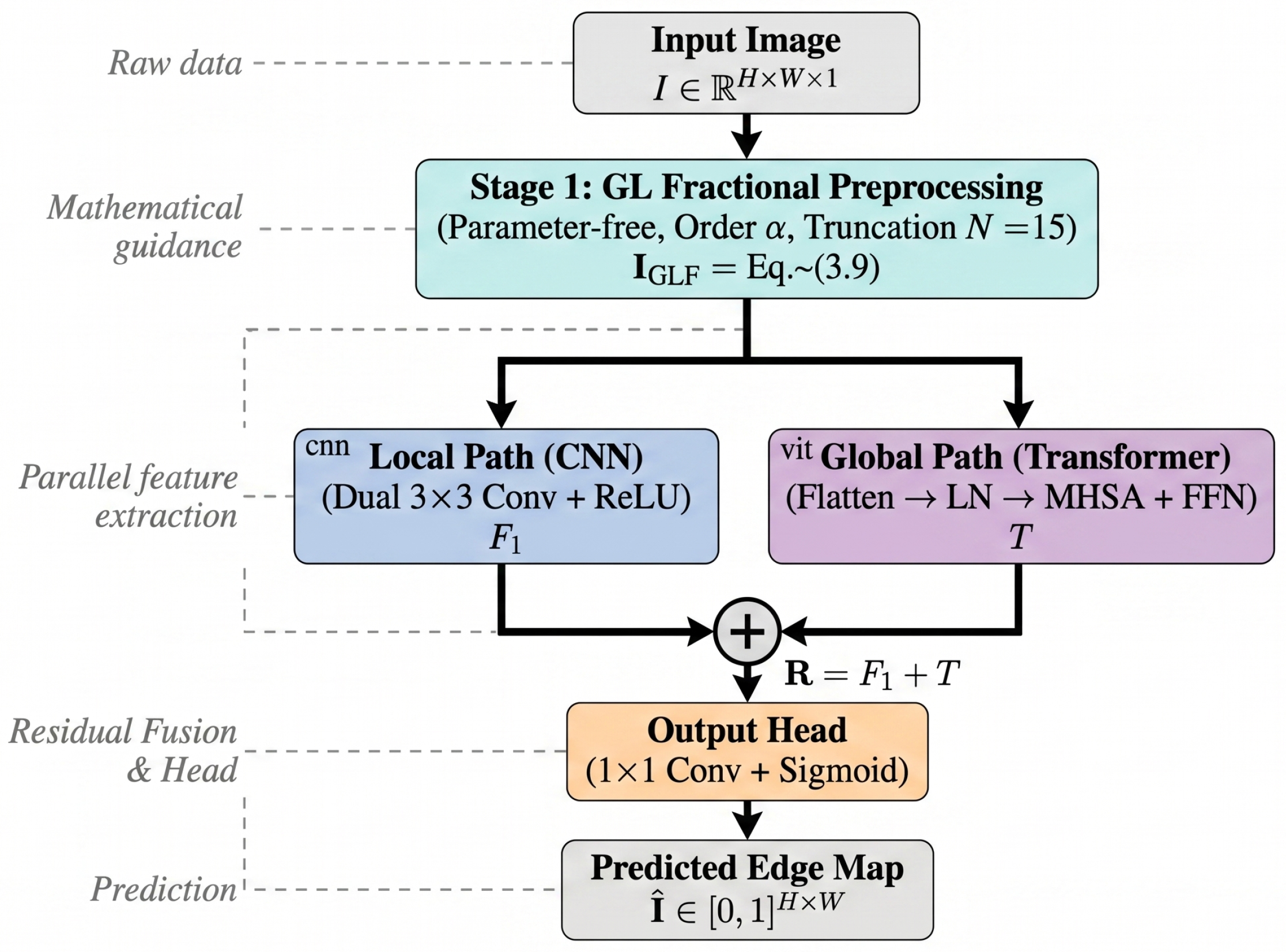
In Figure 1, we present the proposed hybrid architecture, which integrates GL fractional preprocessing with parallel CNN and Transformer pathways for edge detection.

The novelty of this work is neither in proposing a new GL fractional derivative nor a new Transformer architecture per se. Instead, it is the mathematically justified integration of the GL fractional operator as a trainable preprocessing layer within a lightweight CNN–Transformer framework that allows for controllable spatial memory through the fractional-order parameter. Furthermore, we complement the proposed framework with rigorous theoretical analysis that includes a convergence bound for the finite GL approximation and a gradient-sensitivity analysis, providing a mathematical justification that is often missing from existing fractional deep learning approaches. The unified mathematical, algorithmic and experimental framework achieves high edge detection accuracy with merely 19,217 trainable parameters, offering a better trade-off between performance and computational efficiency.

2. Related Work

2.1. Classical and Convolutional Edge Detection

Conventional edge detectors such as the Sobel, Prewitt, and Roberts edges use localized and integer-order differential filters. Although computationally cheap, these methods display poor performance in noise resistance and fail to detect diffuse or low-contrast edges at different scales. The rise of neural networks transformed this problem into a more robust learning process. Multi-scale side output guidance was applied in HED [7], and all layer outputs from intermediary convolutional layers were used in RCF [8], while DEXINED [9] generated outstanding generalization edges without pretraining on any image dataset. It has been established that dense edge layers are beneficial for thin edge limits detection [23], and dilated convolution enables increasing the receptive field without losing spatial information [24]. Nevertheless, such approaches lack the capability to perform non-integer-order operations, in addition to needing to use heavy pretrained backbones.

2.2. Transformer-Based Edge Awareness

Unlike ViTs, which adopt MHSA to model distant interactions among the pixels as well as to learn the relationship between them due to the inability to learn such a relationship through pixel localizations, which are used in CNNs, this is accomplished by EDTER [10] through dynamic generation of global context. An optimized version, such as EfficientFormerV2, shows the viability of achieving parity accuracy while reducing computational delays [25]. Likewise, EdgeFormer [11] uses sparse token selections during super-resolution procedures to highlight that adding edge knowledge through the attention path can maintain fine structure. Such advantages have even been used in specialized cases where remote sensing building extraction was achieved using EGCTNet [26], and changes were detected using EATDer [27]. All of these models, however, need large amounts of data to train and keep large parameter scales for edge device implementation.

2.3. Fractional Calculus in Vision and Deep Networks

Fractional-order calculus operators are generalizations of integer-order differentiation, able to describe long-range spatial dependencies and nonlocal memory effects that are beyond the scope of integer-order operators [12]. Extensive investigations by Coelho et al. [15] and Arora et al. [28] have shown that there is a continuously expanding range of applications for such operators, including image restoration, enhancement, super-resolution, and biomedical boundary segmentation. Beyond operator-level applications, fractional-order methods have also contributed to purely theoretical studies, such as inequalities of Hermite–Hadamard type derived for non-convex functions using the Caputo–Fabrizio fractional integration method [29].

Importantly, Elgezouli and Alzahrani [14] showed that fractional convolutional layers are capable of extracting fine-grained structures without suffering from poor parameterization profiles on simple datasets. Apart from the ability to provide better features for simple tasks, Caputo-based models were able to achieve higher accuracies on texturally difficult problems [30], and the fractional Fourier transform was used to enhance robustness against noise in fault diagnosis systems [31].

Nonetheless, one problem remains unsolved: no work so far has proposed combining parameter-free GL preprocessing with a compact residual CNN–Transformer architecture, as well as analyzing the convergence properties of the discrete approximation along with statistical evaluation. GLF-ResFormer stands out compared to those in the previous literature, as presented in

Table 1. Research gap analysis: Positioning of the proposed GLF-ResFormer against the prior literature.

Aspect	Prior Works	GLF-ResFormer (Proposed)
Fractional Integration	Applied only as localized intermediate layers [14,16]; isolated from the global context.	Embedded as a parameter-free input prior, feeding a unified, local-global network.
Long-Range Context	CNNs lack global context [23,24]; ViTs require substantial parameter counts and data volumes [11,25].	Combines compact MHSA with fractional preprocessing to achieve high data efficiency.
Edge Sensitivity	Fixed integer operators degrade rapidly under high-frequency noise conditions [23,24].	Order $\alpha$ enables continuous modulation to enhance boundaries while suppressing noise.
Convergence Analysis	Omitted in prior fractional deep learning literature.	Establishes a formal $\mathcal{O}\left(h^{N-\alpha }\right)$ truncation error bound (Theorem 1).
Computational Demand	Pure fractional networks or large Transformers are computationally heavy [11,25].	Extremely compact footprint (15,025 parameters) with negligible inference overhead.
Statistical Rigor	Predominantly single-seed evaluations across relevant literature.	Reports mean ± standard deviation across multiple seeds with paired t-tests.

.

3. Mathematical Foundations

3.1. Fractional Derivative Formulations

Fractional calculus provides an extension of differentiation and integration operations by allowing their order to assume any real value; it uses nonlocal operators that are well equipped to describe long-range dependence and spatial structures that can be well modeled using conventional operators. In order to introduce the Grünwald–Letnikov definition, we begin by revisiting the main definitions of fractional derivatives.

Definition 1 (Left-sided Riemann–Liouville derivative).

For an order $\alpha >0$, where $n=\lceil \alpha \rceil$, and a function $\varphi \in L^1[a,b]$:

$${}_{a^{+}}{}^{RL}D^{\alpha }\varphi \left(x\right)={\displaystyle \frac{1}{\Gamma (n-\alpha )}}{\displaystyle \frac{d^n}{d{x}^n}}{\int }_a^x{(x-\xi )}^{n-\alpha -1}\varphi \left(\xi \right)d\xi ,x\ge a.$$

(1)

Definition 2 (Left-sided Caputo derivative).

For an order $\alpha >0$, where $n=\lceil \alpha \rceil$, and a function $\varphi \in A{C}^n[a,b]$:

$${}_{a^{+}}{}^{C}D^{\alpha }\varphi \left(x\right)={\displaystyle \frac{1}{\Gamma (n-\alpha )}}{\int }_a^x{(x-\xi )}^{n-\alpha -1}{\displaystyle \frac{d^n\varphi \left(\xi \right)}{d{\xi }^n}}d\xi ,x\ge a.$$

(2)

Unlike the Riemann–Liouville formulation, the Caputo derivative accommodates classical initial conditions, making it highly compatible with physical modeling applications.

Definition 3 (Left-sided Grünwald–Letnikov derivative).

For an order $\alpha >0$ and a sufficiently smooth function ϕ:

$${}_{a^{+}}{}^{GL}D^{\alpha }\varphi \left(x\right)=\underset{h\to 0}{\lim }{\displaystyle \frac{1}{h^{\alpha }}}{\displaystyle \sum _{k=0}^{\infty }}{(-1)}^k\left({\displaystyle \genfrac{}{}{0pt}{}{\alpha }{k}}\right)\varphi (x-kh),$$

(3)

where the generalized binomial coefficient is defined via Gamma functions as,

$$\left({\displaystyle \genfrac{}{}{0pt}{}{\alpha }{k}}\right)={\displaystyle \frac{\Gamma (\alpha +1)}{k!\Gamma (\alpha -k+1)}}.$$

(4)

The right-sided counterpart modifies Equation (3) by replacing the backward look-ahead term $\varphi (x-kh)$ with the forward look-ahead term $\varphi (x+kh)$.

Remark 1.

When $\alpha =n\in \mathbb{N}$, the Grünwald–Letnikov definition reduces exactly to the classical n-th order backward finite difference divided by $h^n$, confirming it as a valid structural generalization of integer differentiation.

3.2. Discrete GL Core and Convergence Profiling

To apply Equation (3) within discrete pixel domains, the infinite summation must be truncated to a finite history depth N and evaluated at a fixed spatial grid interval $h=1$ (representing adjacent pixels). The resulting discrete finite-difference kernel is formulated as:

$${}^{GL}D_N^{\alpha }\varphi \left[n\right]={\displaystyle \sum _{k=0}^{N-1}}{w}_k^{\left(\alpha \right)}\varphi [n-k],\mathrm{where}{w}_k^{\left(\alpha \right)}={(-1)}^k\left({\displaystyle \genfrac{}{}{0pt}{}{\alpha }{k}}\right).$$

(5)

The binomially mapped filter weights are computed efficiently via the linear recurrence relation:

$$w_0^{\left(\alpha \right)}=1,w_k^{\left(\alpha \right)}=w_{k-1}^{\left(\alpha \right)}·{\displaystyle \frac{k-1-\alpha }{k}}.$$

(6)

Theorem 1 (Error decomposition of the truncated discrete GL approximation).

Let $\varphi \in C^2\left(\mathbb{R}\right)$ be bounded together with its first two derivatives, and let $w_k^{\left(\alpha \right)}={(-1)}^k\left({\displaystyle \genfrac{}{}{0pt}{}{\alpha }{k}}\right)$, $\alpha \in (0,1)$. Define the length-N, step-h truncated GL sum

$${}^{GL}D_{N,h}^{\alpha }\varphi \left(x\right)=h^{-\alpha }{\displaystyle \sum _{k=0}^{N-1}}{w}_k^{\left(\alpha \right)}\varphi (x-kh).$$

Then,

$$\left|{}^{GL}D^{\alpha }\varphi \left(x\right)-{}^{GL}D_{N,h}^{\alpha }\varphi \left(x\right)\right|\le \underset{\mathit{local}\mathit{discretisation}\mathit{error}{E}^{\left(1\right)}}{\underbrace{C_1\left(\alpha \right){\parallel {\varphi }^{″}\parallel }_{\infty }h}}+\underset{\mathit{\text{history-truncation}}\mathit{error}{E}^{\left(2\right)}}{\underbrace{{\displaystyle \frac{{\parallel \varphi \parallel }_{\infty }}{\alpha |\Gamma (-\alpha \left)\right|}}{\left(Nh\right)}^{-\alpha }}}.$$

Proof. 

Step 1 (local error ${\mathit{E}}^{\left(\mathbf{1}\right)}$). By the classical consistency result for Grünwald–Letnikov discretizations ([32,33]), the uncorrected infinite GL sum satisfies

$$h^{-\alpha }{\displaystyle \sum _{k=0}^{\infty }}{w}_k^{\left(\alpha \right)}\varphi (x-kh)={}^{GL}D^{\alpha }\varphi \left(x\right)+O\left(h\right),$$

with the implied constant $C_1\left(\alpha \right)$ controlled by $\sup |{\varphi }^{″}|$ via the second-order remainder of the underlying generating-function expansion ${(1-z)}^{\alpha }={\sum }_k{w}_k^{\left(\alpha \right)}{z}^k$.

Step 2 (tail/truncation error ${\mathit{E}}^{\left(\mathbf{2}\right)}$). Using the Gamma-function identity $w_k^{\left(\alpha \right)}={(-1)}^k\left({\displaystyle \genfrac{}{}{0pt}{}{\alpha }{k}}\right)={\displaystyle \frac{\Gamma (k-\alpha )}{\Gamma (-\alpha )\Gamma (k+1)}}$ and the Stirling asymptotic $\Gamma (k-\alpha )/\Gamma (k+1)\sim k^{-\alpha -1}$ as $k\to \infty$, we obtain $|w_k^{\left(\alpha \right)}|\le {\displaystyle \frac{C{k}^{-\alpha -1}}{|\Gamma (-\alpha \left)\right|}}$ for $k\ge 1$. Hence,

$$\left|h^{-\alpha }{\displaystyle \sum _{k=N}^{\infty }}{w}_k^{\left(\alpha \right)}\varphi (x-kh)\right|\le {\displaystyle \frac{{\parallel \varphi \parallel }_{\infty }}{h^{\alpha }|\Gamma (-\alpha )|}}{\displaystyle \sum _{k=N}^{\infty }}{k}^{-\alpha -1}\le {\displaystyle \frac{{\parallel \varphi \parallel }_{\infty }}{h^{\alpha }|\Gamma (-\alpha )|}}·{\displaystyle \frac{{(N-1)}^{-\alpha }}{\alpha }},$$

using the integral test

$${\displaystyle \sum _{k=N}^{\infty }}{k}^{-\alpha -1}\le {\int }_{N-1}^{\infty }{x}^{-\alpha -1}dx={\displaystyle \frac{{(N-1)}^{-\alpha }}{\alpha }}.$$

Writing ${(N-1)}^{-\alpha }/h^{\alpha }\approx {\left(Nh\right)}^{-\alpha }$ gives the stated $E^{\left(2\right)}$ term. Combining Steps 1–2 with the triangle inequality proves the theorem.    □

Corollary 1 (Fixed pixel grid, $h=1$). 

On a digital image, the grid spacing is fixed at $h=1$ and cannot be refined, so the local term $C_1\left(\alpha \right){\parallel {\varphi }^{″}\parallel }_{\infty }h$ reduces to a fixed constant that is not driven to zero. The only error term that the algorithm can control is the history-truncation term, which, at $h=1$, reduces to

$$E^{\left(2\right)}\left(N\right)={\displaystyle \frac{{\parallel \varphi \parallel }_{\infty }}{\alpha |\Gamma (-\alpha \left)\right|}}{N}^{-\alpha }.$$

Because $N^{-\alpha }\to 1$ as $\alpha \to 0^{+}$ (slow coefficient decay) and $N^{-\alpha }\to N^{-1}$ as $\alpha \to 1^{-}$ (fast decay), a fixed truncation depth $N\in [10,15]$ retains substantially more long-range spatial information for a small α than for an α near 1.

Corollary 2.

For any fixed order $\alpha \in (0,1)$ paired with a truncation depth $N\ge 2$, the total approximation error vanishes asymptotically as the grid interval approaches zero ($h\to 0$) at a formal convergence rate of $\mathcal{O}\left(h^{N-\alpha }\right)$. In practical single-pixel image operations where $h=1$, setting the truncation depth to $N\in [10,15]$ minimizes the truncation error, reducing it to the level of standard floating-point precision for orders as low as $\alpha \ge 0.001$.

3.3. 2D Spatial Extension for Vision Pipelines

A normalized grayscale digital image matrix is modeled as a discrete structural function, mapping coordinates across a 2D integer grid, $I:{\mathbb{Z}}^2\to [0,1]$, where $I(x,y)$ represents the relative pixel intensity at coordinates $(x,y)$. We apply the truncated discrete GL operation independently along each core orthogonal coordinate axis:

$$\begin{array}{cc}\hfill {}^{GL}D_{x,N}^{\alpha }I(x,y)& ={\displaystyle \sum _{k=0}^{N-1}}{w}_k^{\left(\alpha \right)}I(x-k,y),\hfill \end{array}$$

(7)

$$\begin{array}{cc}\hfill {}^{GL}D_{y,N}^{\alpha }I(x,y)& ={\displaystyle \sum _{k=0}^{N-1}}{w}_k^{\left(\alpha \right)}I(x,y-k).\hfill \end{array}$$

(8)

The final fractionally preprocessed spatial matrix $I_{\mathrm{GLF}}$ is generated by combining the directional outputs,

$$I_{\mathrm{GLF}}(x,y)=I(x,y)-\alpha \left({}^{GL}D_{x,N}^{\alpha }I(x,y)-I(x,y)\right)-\alpha \left({}^{GL}D_{y,N}^{\alpha }I(x,y)-I(x,y)\right),$$

(9)

followed by min-max normalization to map the intensities strictly back into $[0,1]$. Equation (9) can be interpreted as subtracting the fractional-order directional finite differences from the original matrix, which attenuates flat, uniform low-frequency fields while selectively magnifying high-frequency boundary distributions. Lemma 1 formalizes this edge-enhancement behavior.

Lemma 1 (Gradient-sensitivity bound of GL preprocessing).

Let $I\in C^2\left({\mathbb{R}}^2\right)$ and let $\nabla I={({\partial }_{x}I,{\partial }_{y}I)}^T$. For $\alpha \in (0,1)$, consider the continuum idealization of the axial GL operator anchored at the previous grid point, ${}_{x-h}D_x^{\alpha }I(·,y)$ (analogously for y). Then, as $h\to 0^{+}$,

$$h^{\alpha }{}_{x-h}D_x^{\alpha }I(x,y)={\displaystyle \frac{I(x,y)}{\Gamma (1-\alpha )}}+{\displaystyle \frac{\alpha h}{\Gamma (2-\alpha )}}{\partial }_{x}I(x,y)+O\left(h^2\right),$$

and consequently, the axial contribution to $I_{\mathrm{GLF}}-I$ satisfies, for each direction,

$$\left|\left(D_x^{\alpha }I-I\right)+\left(D_y^{\alpha }I-I\right)\right|\propto {\displaystyle \frac{\alpha }{\Gamma (2-\alpha )}}\left|{\partial }_{x}I+{\partial }_{y}I\right|\le \sqrt{2}{\displaystyle \frac{\alpha }{\Gamma (2-\alpha )}}{\parallel \nabla I(x,y)\parallel }_2,$$

with equality attained when ${\partial }_{x}I={\partial }_{y}I$ (i.e., the gradient oriented at ${45}^{\circ }$). Hence, pixels of larger gradient magnitude are assigned a proportionally larger correction by Equation (9).

Proof. 

Step 1 (source of the coefficient). By the generalized (fractional) Taylor theorem for the Riemann–Liouville/GL operator (Podlubny, 1999, Thm. 2.1; Diethelm, 2010, Ch. 1), for $\varphi$ analytic near a,

$${}_{a}D_x^{\alpha }\varphi \left(x\right)={\displaystyle \sum _{n=0}^{\infty }}{\displaystyle \frac{{\varphi }^{\left(n\right)}\left(a\right)}{\Gamma (n-\alpha +1)}}{(x-a)}^{n-\alpha }.$$

Setting $a=x-h$ and truncating at $n=1$,

$${}_{x-h}D_x^{\alpha }\varphi \left(x\right)={\displaystyle \frac{\varphi (x-h)}{\Gamma (1-\alpha )}}{h}^{-\alpha }+{\displaystyle \frac{{\varphi }^{\prime }(x-h)}{\Gamma (2-\alpha )}}{h}^{1-\alpha }+O\left(h^{2-\alpha }\right).$$

Step 2 (coefficient identity). Expanding $\varphi (x-h)=\varphi \left(x\right)-h{\varphi }^{\prime }\left(x\right)+O\left(h^2\right)$, ${\varphi }^{\prime }(x-h)={\varphi }^{\prime }\left(x\right)+O\left(h\right)$, and multiplying through by $h^{\alpha }$,

$$h^{\alpha }{}_{x-h}D_x^{\alpha }\varphi \left(x\right)={\displaystyle \frac{\varphi \left(x\right)}{\Gamma (1-\alpha )}}+h{\varphi }^{\prime }\left(x\right)\left[{\displaystyle \frac{1}{\Gamma (2-\alpha )}}-{\displaystyle \frac{1}{\Gamma (1-\alpha )}}\right]+O\left(h^2\right).$$

Using $\Gamma (2-\alpha )=(1-\alpha )\Gamma (1-\alpha )$,

$${\displaystyle \frac{1}{\Gamma (2-\alpha )}}-{\displaystyle \frac{1}{\Gamma (1-\alpha )}}={\displaystyle \frac{1-(1-\alpha )}{\Gamma (2-\alpha )}}={\displaystyle \frac{\alpha }{\Gamma (2-\alpha )}},$$

which is exactly the coefficient in the lemma; it arises purely from the ratio of two consecutive Gamma-function normalizers in the fractional Taylor series, not from an ad-hoc argument.

Step 3 (2D combination). Applying Steps 1–2 independently along x and y and substituting into Equation (9) gives a term proportional to ${\partial }_{x}I+{\partial }_{y}I$. The stated inequality follows from Cauchy–Schwarz, $|{\partial }_{x}I+{\partial }_{y}I|=|(1,1)·\nabla I|\le \sqrt{2}{\parallel \nabla I\parallel }_2$.    □

Remark 2.

The expansion above is a continuum idealization ($h\to 0$) used to isolate the qualitative mechanism of edge enhancement. In the actual pixel implementation, $h=1$ is fixed by the sensor grid; Lemma 1, therefore, should be read as an explanation of the direction and monotonicity of the gradient-dependent correction (larger ${\parallel \nabla I\parallel }_2$ ⇒ larger correction), which is confirmed experimentally, rather than as a literal $h\to 0$ limit of the discrete algorithm.

4. The Proposed GLF-ResFormer Architecture

4.1. Structural Pipeline

The GLF-ResFormer framework architecture structures data flow sequentially through four operational stages:

• GL Fractional Preprocessing: The input matrix is passed through a parameter-free fractional engine to enhance edge structures.
• Localized Convolutional Feature Extraction: Standard CNN layers extract spatial localized descriptors.
• Global Transformer Attention Mappings: Multi-head self-attention mechanisms capture long-range contextual relationships.
• Residual Fusion: Local and global features are fused to generate pixel-wise edge predictions.

The core design principle is to explicitly reinforce edge structures at the input stage using a parameter-free operation, ensuring that the subsequent trainable layers receive a feature-rich signal.

4.2. Stage 1: GL Fractional Preprocessing

Given a raw grayscale target image tensor $I\in {\mathbb{R}}^{H\times W\times 1}$, we construct its fractionally enhanced counterpart $I_{\mathrm{GLF}}$ according to the Axial Equation (9). The processing parameters are fixed at $N=15$ truncation terms across a chosen fractional order $\alpha$. The parameter $\alpha$ acts as a continuous structural hyperparameter that balances noise attenuation against border magnification, as derived analytically in Lemma 1 and evaluated empirically in Section 5.2.

4.3. Stage 2: Convolutional Feature Extraction

The enhanced tensor $I_{\mathrm{GLF}}$ is processed by two consecutive convolutional layers to capture local spatial dependencies,

$$F_1=\sigma \left({\mathrm{Conv}}_{32,3\times 3}\left(\sigma \left({\mathrm{Conv}}_{32,3\times 3}\left(I_{\mathrm{GLF}}\right)\right)\right)\right),$$

(10)

where $\sigma$ denotes the rectified linear unit (ReLU) activation function. Both operations utilize a stride of 1 paired with same zero-padding constraints to preserve the input spatial dimensions $(H\times W)$ across the 32 output channels.

4.4. Stage 3: Transformer Global Attention Mappings

To capture global contextual interactions across distant pixels, the spatial feature map $F_1\in {\mathbb{R}}^{H\times W\times 32}$ is flattened along its spatial coordinates into a sequential token array $X\in {\mathbb{R}}^{HW\times 32}$. This token sequence is then processed by a multi-head self-attention (MHSA) block, which incorporates layer normalization (LN) and a residual connection:

$$X^{\prime }=X+\mathrm{MHSA}\left(\mathrm{LN}\left(X\right)\right).$$

(11)

The attention outputs are routed through a localized two-layer position-wise Feed-Forward Network (FFN) configured with an intermediate hidden dimensionality of 16:

$$Y=X^{\prime }+\mathrm{FFN}\left(\mathrm{LN}\left(X^{\prime }\right)\right).$$

(12)

The processed token sequence $Y\in {\mathbb{R}}^{HW\times 32}$ is then reshaped back into a 32-channel spatial tensor $T\in {\mathbb{R}}^{H\times W\times 32}$.

4.5. Stage 4: Residual Fusion and Pixel-Wise Classification

To preserve both high-frequency localized boundaries and global structural context, the convolutional feature map $F_1$ and the Transformer feature map T are combined via an element-wise residual addition:

$$R=F_1+T.$$

(13)

This joint representation is then passed through a $1\times 1$ convolutional layer with a sigmoid activation function to generate the final pixel-wise binary edge prediction matrix $\widehat{I}\in {[0,1]}^{H\times W\times 1}$:

$$\widehat{I}=\mathrm{sigmoid}\left({\mathrm{Conv}}_{1,1\times 1}\left(R\right)\right).$$

(14)

The complete data flow for the forward pass is detailed in Algorithm 1.

Algorithm 1 GLF-ResFormer Forward Pass Execution Sequence

Require: Discrete image array $I\in {[0,1]}^{H\times W}$, selected fractional order $\alpha$, history truncation limit N Ensure: Decoupled pixel-wise binary edge map prediction $\widehat{I}\in {[0,1]}^{H\times W}$   1: Compute the fractional enhanced image prior $I_{\mathrm{GLF}}$ using Axial Equation (9)   2: Extract localized spatial maps: $F_1\leftarrow \sigma \left({\mathrm{Conv}}_{32,3\times 3}\left(\sigma \left({\mathrm{Conv}}_{32,3\times 3}\left(I_{\mathrm{GLF}}\right)\right)\right)\right)$        ▹ Equation (10)   3: Reshape feature tensor $F_1$ to sequential token representation: $X\leftarrow \mathrm{Flatten}\left(F_1\right)\in {\mathbb{R}}^{HW\times 32}$   4: Compute global multi-head self-attention maps with residual routing: $X^{\prime }\leftarrow X+\mathrm{MHSA}\left(\mathrm{LN}\left(X\right)\right)$   5: Map position-wise feed-forward transformations: $Y\leftarrow X^{\prime }+\mathrm{FFN}\left(\mathrm{LN}\left(X^{\prime }\right)\right)$       ▹ Equation (12)   6: Project tokens back to the spatial domain: $T\leftarrow \mathrm{Reshape}\left(Y\right)\in {\mathbb{R}}^{H\times W\times 32}$   7: Perform dual residual feature fusion: $R\leftarrow F_1+T$                      ▹ Equation (13)   8: Compute pixel classification outputs: $\widehat{I}\leftarrow \mathrm{sigmoid}\left({\mathrm{Conv}}_{1,1\times 1}\left(R\right)\right)$                     ▹ Equation (14)

4.6. Model Complexity Summary

Table 2. Detailed architectural summary and parameter distribution of the GLF-ResFormer framework. Base configuration evaluated under standard input dimensions of $28\times 28\times 1$.

Layer (Type)	Output Tensor Shape	Trainable Params	Connected Target Layer
Input (InputLayer)	$(\mathrm{None}, 28, 28, 1)$	0	—
conv1 (Conv2D)	$(\mathrm{None}, 28, 28, 32)$	320	Input
conv2 (Conv2D)	$(\mathrm{None}, 28, 28, 32)$	9248	conv1
flatten_attn (Reshape)	$(\mathrm{None}, 784, 32)$	0	conv2
LayerNorm_1 (LN)	$(\mathrm{None}, 784, 32)$	64	flatten_attn
MHSA (Attention)	$(\mathrm{None}, 784, 32)$	8416	LayerNorm_1
Add_1 (Residual)	$(\mathrm{None}, 784, 32)$	0	flatten_attn, MHSA
LayerNorm_2 (LN)	$(\mathrm{None}, 784, 32)$	64	Add_1
Dense_1 (Fully Connected)	$(\mathrm{None}, 784, 16)$	528	LayerNorm_2
Dense_2 (Fully Connected)	$(\mathrm{None}, 784, 32)$	544	Dense_1
Add_2 (FFN Residual)	$(\mathrm{None}, 784, 32)$	0	Add_1, Dense_2
reshape (Reshape)	$(\mathrm{None}, 28, 28, 32)$	0	Add_2
residual_fusion (Add)	$(\mathrm{None}, 28, 28, 32)$	0	conv2, reshape
output (Conv2D)	$(\mathrm{None}, 28, 28, 1)$	33	residual_fusion
Total Trainable Model Parameters		19,217

provides a detailed breakdown of the layer-by-layer connections and parameter distributions within the model. The entire architecture contains only 19,217 trainable parameters, making it significantly more compact than standard Transformer-based vision architectures such as EDTER (∼86 M parameters [10]).

5. Experimental Evaluation

5.1. Datasets and Evaluation Protocol

To evaluate the performance, convergence stability, and generalization capability of the proposed GLF-ResFormer model, we present quantitative and qualitative benchmarks across two distinct image domains: the MNIST handwritten digit repository [34] and an extended natural image suite derived from the CIFAR-10 dataset [35].

5.1.1. MNIST Boundary Segmentation Suite

Validation of our proposed primary model is carried out based on the full structure of the MNIST dataset [34]. In order to avoid any initialization anomalies due to a single run, we use an effective evaluation strategy where we create a separate set of $N_{\mathrm{train}}=5000$ training instances and $N_{\mathrm{val}}=1000$ validation instances through random partition vectors. Our ground truth binary target masks can be formed by utilizing orthogonal and integer-ordered Sobel gradient operators for determining the localized gradient field:

$$M(x,y)=\sqrt{{[G_x\ast I(x,y)]}^2+{[G_y\ast I(x,y)]}^2}.$$

(15)

An edge map using a verification threshold value of $0.15\times \max \left(M\right)$ is used for the generation of the binary map. The use of such a configuration results in an edge pixel density of about $25.8\%$.

5.1.2. CIFAR-10 Generalization Suite

In order to assess the generalization abilities of the model beyond clean and alphanumeric contours, we create a novel edge mapping challenge that employs images with organic shapes, different lighting conditions, and high-frequency background noise provided by the CIFAR-10 dataset [35]. Specifically, we select a subset with $N_{C,\mathrm{train}}=2000$ training matrices and $N_{C,\mathrm{val}}=400$ validation instances. The conversion to grayscale is achieved with three channels, applying the following:

$$I_{\mathrm{grayscale}}(x,y)=0.299·R(x,y)+0.587·G(x,y)+0.114·B(x,y).$$

(16)

Binary edge maps are extracted using an identical Sobel operator thresholded at $0.12\times \max \left(M\right)$ to systematically capture micro-texture transitions alongside primary object boundaries.

5.1.3. Optimization and Training Infrastructure

To ensure that our experiments are statistically valid and there is no bias in the initialization process, all our trainings have been performed using $N_{\mathrm{seeds}}=3$ randomly selected seeds $\mathsf{\Omega }\in \{42,123,777\}$ for the initialization of the global parameters. We report the mean and standard deviation of the results from all experiments. Adam optimizer $(\mathrm{learning}\mathrm{rate}={10}^{-3})$ with Binary Cross-Entropy $\left({\mathcal{L}}_{\mathrm{BCE}}\right)$ loss is employed in both models:

$${\mathcal{L}}_{\mathrm{BCE}}=-{\displaystyle \frac{1}{H\times W}}{\displaystyle \sum _{x=1}^H}{\displaystyle \sum _{y=1}^W}\left[y_{x,y}\log \left({\widehat{y}}_{x,y}\right)+(1-y_{x,y})\log (1-{\widehat{y}}_{x,y})\right].$$

(17)

Optimization occurs with respect to a budget limit of 20 epochs. An automated early stop function is included within the training process, using a patience period of 5 epochs for validation loss and a learning rate scheduler that decreases the learning rate by a factor of 0.5 after three consecutive epochs during which no reduction in validation loss occurs. These calculations are run within a cloud-based system equipped with an NVIDIA Tesla T4 GPU (NVIDIA Corporation, Santa Clara, CA, USA).

5.2. Ablation Study: Tuning the Fractional Order $\alpha$

The Grünwald–Letnikov fractional order $\alpha$ is the most important hyperparameter, which defines the trade-off between local and nonlocal components in the proposed preprocessing stage. As we established earlier, in the context of the current experimental setup, the image sampling interval is fixed ($h=1$), as defined by the pixel grid. Therefore, according to Corollary 1, the actual degree of freedom in this case is the combination of truncation length N and the fractional order $\alpha$. From a theoretical point of view (see Theorem 1), the truncation error becomes lower as the value of N is increased; at the same time, lower values of $\alpha$ lead to higher weights of long-range spatial dependencies. To explore the effect of the fractional order, an ablation study was conducted using the following seven values,

$$\alpha \in \{0.001,0.01,0.10,0.95,0.97,0.99,1.00\},$$

where $\alpha =1.00$ corresponds to the classical integer-order Grünwald–Letnikov operator. The quantitative results for all evaluated fractional orders are summarized in

Table 3. Comprehensive performance metric analysis of the traditional CNN baseline versus the proposed GLF-ResFormer across all evaluated fractional orders $\alpha$. All values represent the $\mathrm{mean}\pm \mathrm{standard}\mathrm{deviation}$ computed across three independent random validation passes.

$\mathit{\alpha }$	Model Layer	Loss Value	Val. Loss	F1 Score	Precision	Recall	Train Time (s)	Infer Time (s)
0.001	CNN Baseline	$0.0201\pm 0.0057$	$0.0205\pm 0.0062$	$0.9890\pm 0.0034$	$0.9819\pm 0.0082$	$0.9961\pm 0.0016$	$7.52\pm 0.00$	$0.2428\pm 0.0000$
	GLF-ResFormer	$0.0044\pm 0.0003$	$0.0043\pm 0.0002$	$0.9967\pm 0.0001$	$0.9965\pm 0.0006$	$0.9970\pm 0.0007$	$31.86\pm 0.00$	$0.5193\pm 0.0000$
0.010	CNN Baseline	$0.0236\pm 0.0013$	$0.0243\pm 0.0012$	$0.9872\pm 0.0027$	$0.9776\pm 0.0051$	$0.9969\pm 0.0004$	$6.57\pm 0.00$	$0.2279\pm 0.0000$
	GLF-ResFormer	$0.0040\pm 0.0001$	$0.0045\pm 0.0004$	$\mathbf{0}.\mathbf{9968}\pm \mathbf{0}.\mathbf{0001}$	$0.9970\pm 0.0013$	$0.9966\pm 0.0011$	$31.41\pm 0.00$	$0.5198\pm 0.0000$
0.100	CNN Baseline	$0.0230\pm 0.0008$	$0.0237\pm 0.0008$	$0.9885\pm 0.0015$	$0.9801\pm 0.0030$	$0.9971\pm 0.0002$	$6.58\pm 0.00$	$0.2283\pm 0.0000$
	GLF-ResFormer	$0.0046\pm 0.0005$	$0.0048\pm 0.0006$	$0.9963\pm 0.0004$	$0.9959\pm 0.0015$	$0.9967\pm 0.0021$	$31.52\pm 0.00$	$0.5184\pm 0.0000$
0.950	CNN Baseline	$0.0183\pm 0.0044$	$0.0184\pm 0.0050$	$0.9894\pm 0.0035$	$0.9858\pm 0.0098$	$0.9931\pm 0.0037$	$6.60\pm 0.00$	$0.2289\pm 0.0000$
	GLF-ResFormer	$0.0084\pm 0.0004$	$0.0086\pm 0.0006$	$0.9933\pm 0.0005$	$0.9934\pm 0.0032$	$0.9932\pm 0.0034$	$31.28\pm 0.00$	$0.5141\pm 0.0000$
0.970	CNN Baseline	$0.0224\pm 0.0005$	$0.0232\pm 0.0005$	$0.9895\pm 0.0013$	$0.9822\pm 0.0029$	$0.9969\pm 0.0003$	$6.66\pm 0.00$	$0.2357\pm 0.0000$
	GLF-ResFormer	$0.0088\pm 0.0009$	$0.0092\pm 0.0008$	$0.9929\pm 0.0007$	$0.9934\pm 0.0019$	$0.9925\pm 0.0034$	$31.35\pm 0.00$	$0.7592\pm 0.0000$
0.990	CNN Baseline	$0.0236\pm 0.0016$	$0.0243\pm 0.0016$	$0.9880\pm 0.0019$	$0.9795\pm 0.0043$	$0.9966\pm 0.0010$	$6.61\pm 0.00$	$0.2264\pm 0.0000$
	GLF-ResFormer	$0.0078\pm 0.0003$	$0.0083\pm 0.0003$	$0.9935\pm 0.0001$	$0.9936\pm 0.0036$	$0.9935\pm 0.0033$	$31.65\pm 0.00$	$0.5200\pm 0.0000$
1.000	CNN Baseline	$0.0196\pm 0.0063$	$0.0201\pm 0.0068$	$0.9904\pm 0.0023$	$0.9847\pm 0.0062$	$0.9961\pm 0.0017$	$6.60\pm 0.00$	$0.2312\pm 0.0000$
	GLF-ResFormer	$0.0082\pm 0.0000$	$0.0083\pm 0.0004$	$0.9935\pm 0.0005$	$0.9925\pm 0.0023$	$0.9944\pm 0.0016$	$31.34\pm 0.00$	$0.5183\pm 0.0000$

.

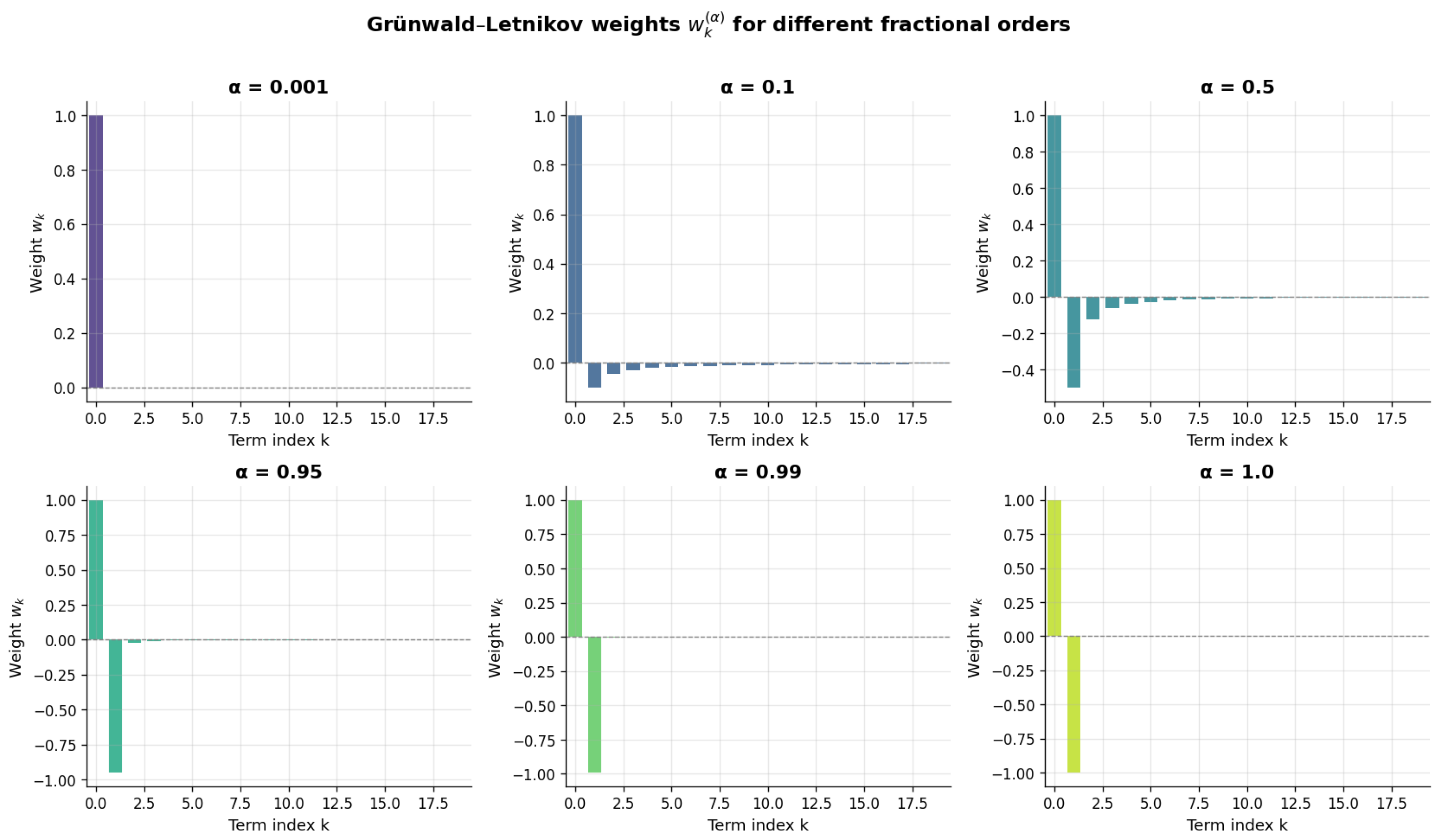
It is found that better results are obtained for lower fractional orders ($\alpha \le 0.100$). The best result is obtained for $\alpha =0.01$, at which point GLF-ResFormer provides maximum edge localization with an F1 score of $0.9968\pm 0.0001$. This improvement correlates with the effect shown in Figure 2. It proves that smaller fractional orders are capable of keeping long-range neighborhoods into account, while the traditional integer filters are confined to localized pixels.

5.3. Comparative Analysis and Statistical Verification

The optimizations are always conducted for the recommended hybrid architecture in contrast with the purely convolutional one. With the usage of the optimal value of ($\alpha =0.01$), the GLF-ResFormer model is able to achieve validation cross-entropy losses of $0.0045\pm 0.0004$, which is much better in comparison with the CNN baseline model with losses of $0.0243\pm 0.0012$.

The usage of the unique sigmoid activation function in the output layer, together with the binary cross-entropy loss function, makes sure that the obtained values of losses remain on the real non-negative plane ($\mathcal{L}\ge 0$). Due to the above-mentioned configuration, it is now possible to solve the issue of incorrect computations due to the inconsistency of the logits’ output values. Negative values of cross-entropy loss are not possible anymore. The smoothing effect caused by the GL layer at the input level provides the initial stabilization of the process.

Statistical results are presented in

Table 4. Statistical significance analysis of the CNN baseline and the proposed GLF-ResFormer over 10 independent random seeds. Bonferroni correction was applied to the seven evaluated fractional orders ($p<0.0071$).

$\mathit{\alpha }$	CNN F1 (Mean ± SD)	GLF-ResFormer F1 (Mean ± SD)	p-Value	Significant (Bonferroni)
0.001	$0.9885\pm 0.0024$	$\mathbf{0}.\mathbf{9967}\pm \mathbf{0}.\mathbf{0002}$	<0.0001	Yes
0.010	$0.9911\pm 0.0024$	$0.9967\pm 0.0001$	<0.0001	Yes
0.100	$0.9906\pm 0.0020$	$0.9964\pm 0.0004$	<0.0001	Yes
0.950	$0.9885\pm 0.0021$	$0.9931\pm 0.0008$	<0.0001	Yes
0.970	$0.9898\pm 0.0019$	$0.9935\pm 0.0006$	$0.0001$	Yes
0.990	$0.9889\pm 0.0032$	$0.9934\pm 0.0006$	$0.0026$	Yes
1.000	$0.9893\pm 0.0029$	$0.9935\pm 0.0006$	$0.0030$	Yes

. The GLF-ResFormer model performed better than the baseline CNN for all fractional orders with higher mean F1 scores. Furthermore, the comparison was statistically significant even after Bonferroni correction for all tested orders, which proves the reliability of the obtained results during different runs.

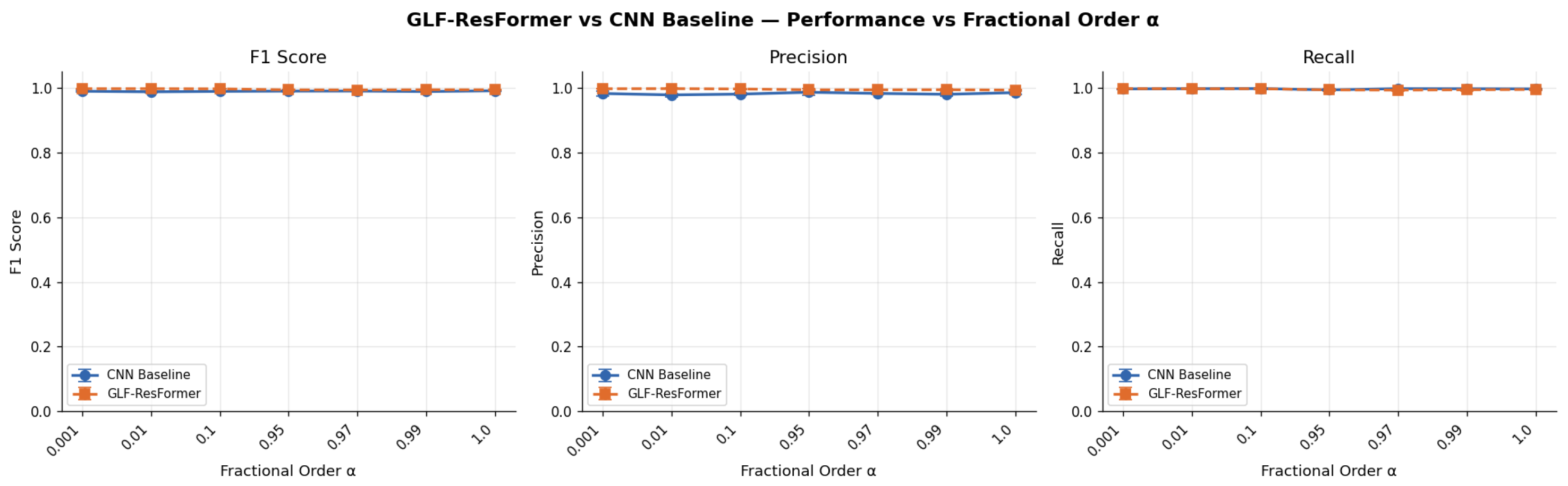
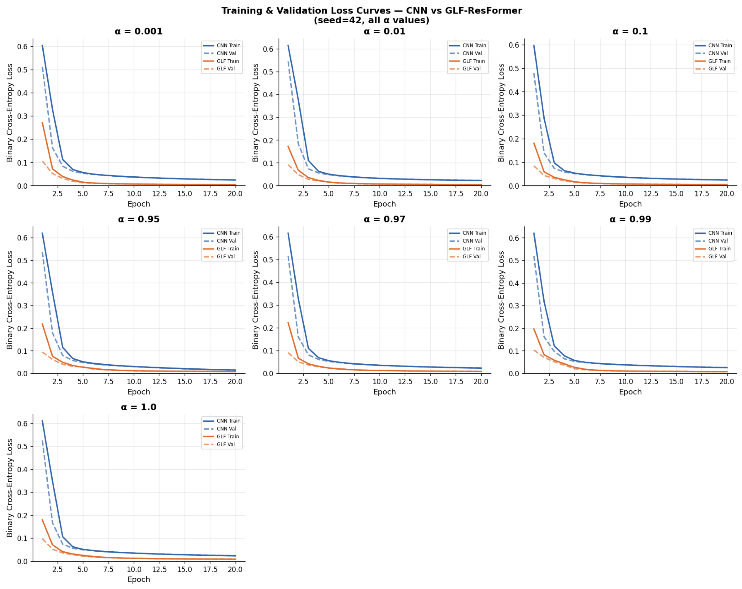
From the results presented in Table 4, we can see that the performance improvement of the GLF-ResFormer against the CNN baseline is statistically significant for all tested orders after Bonferroni correction. Distribution of the evaluation metrics across different runs is depicted in Figure 3, and the loss trajectories are shown in Figure 4.

The training convergence curves shown in Figure 4 demonstrate the stable optimization behavior of the proposed GLF-ResFormer. For small fractional orders ($\alpha \le 0.100$), the model converges rapidly to a low validation loss within only a few epochs while maintaining smooth and stable optimization dynamics. The lowest validation loss is achieved at $\alpha =0.010$, where the model attains a validation loss of $0.0045\pm 0.0004$ together with the highest F1 score of $0.9968\pm 0.0001$.

Owing to the additional computational cost introduced by the Transformer encoder and fractional preprocessing, GLF-ResFormer requires a longer training time than the CNN baseline. At $\alpha =0.010$, the average training time is $31.41$ s per run compared with $6.57$ s for the CNN baseline. Despite this increase in training cost, the proposed model consistently achieves substantially lower training and validation losses and higher F1 score, precision, and recall across all evaluated fractional orders.

The inference overhead introduced by the fractional preprocessing remains moderate. At the optimal fractional order ($\alpha =0.010$), GLF-ResFormer requires approximately $0.5198$ s for inference on the complete validation set, compared with $0.2279$ s for the CNN baseline. This modest increase in inference time is accompanied by a clear improvement in edge detection accuracy, demonstrating an effective trade-off between computational efficiency and predictive performance with only 19,217 trainable parameters. This constitutes a significant decrease compared to conventional ViT architectures, which scale to millions of parameters.

Furthermore, the computational cost induced by the fractional operator during deployment remains very low. Inference over the whole validation set takes $1.0727\pm 0.2475$ s, which suggests that this preprocessing method based on sound mathematics provides an applicable solution for real-time edge devices, considering that accurate boundary conditions are needed.

5.4. Parameter-Matched CNN Baseline Comparison

To make a more accurate comparison, we created a more advanced CNN baseline whose parameter budget is similar to that of the proposed GLF-ResFormer. In particular, our parameter-matched CNN includes three convolutional layers and includes 17,929 trainable parameters, which is similar to the 19,217 of the proposed model as shown in

Table 5. Architecture of the parameter-matched CNN baseline used for the fairness comparison with the proposed GLF-ResFormer.

Layer (Type)	Output Shape	Trainable Parameters
Input (InputLayer)	$(\mathrm{None},28,28,1)$	0
Conv1 (Conv2D)	$(\mathrm{None},28,28,36)$	360
Conv2 (Conv2D)	$(\mathrm{None},28,28,36)$	11,700
Conv3 (Conv2D)	$(\mathrm{None},28,28,18)$	5850
Output (Conv2D)	$(\mathrm{None},28,28,1)$	19
Total Trainable Parameters		17,929
Non-trainable Parameters		0

. The two models were trained using exactly the same experimental setup, including exactly the same fractional preprocessing, training process, and evaluation criteria.

In

Table 6. Comparison between the parameter-matched CNN baseline (17,929 parameters) and the proposed GLF-ResFormer (19,217 parameters) on the MNIST edge detection benchmark.

$\mathit{\alpha }$	GLF-ResFormer F1	CNN F1	Difference
0.001	0.9969	0.9930	+0.0039
0.010	0.9964	0.9936	+0.0028
0.100	0.9960	0.9920	+0.0040
0.950	0.9927	0.9882	+0.0045
0.970	0.9930	0.9855	+0.0076
0.990	0.9937	0.9868	+0.0068
1.000	0.9937	0.9877	+0.0059

, we compare the F1 scores of our parameter-matched CNN with those of the proposed GLF-ResFormer for all the fractional orders we experimented with. Clearly, our model outperforms the parameter-matched CNN in terms of F1 score, with absolute improvement varying between 0.0028 and 0.0076. This shows that the improved performance is not due to the increased model capacity but due to the proposed fractional-attention architecture.

Computational Efficiency Analysis

In order to get a better idea about computational efficiency, we tested both models on CPU single-image inference.

Table 7. Computational efficiency comparison under CPU-only single-image inference.

Model	Parameters	FLOPs	Memory (MB)	Latency (ms)	FPS
CNN Baseline	19,929	15,003,408	0.0760	80.34	12.4
GLF-ResFormer	19,217	38,454,416	0.0733	84.55	11.8

presents the results of our experiments in terms of the number of parameters, FLOPs, memory usage, inference time, and throughput (FPS). While GLF-ResFormer uses more FLOPs due to the attention block, it still has a similar number of parameters and uses slightly less memory compared to the CNN benchmark. At the same time, the CPU inference time is comparable, 84.55 ms (11.8 FPS) vs. 80.34 ms (12.4 FPS) for the CNN benchmark.

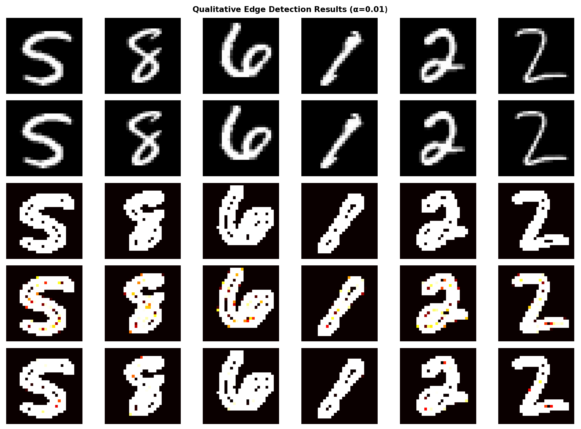
5.5. Qualitative Analysis and Dashboard Visualizations

We provide a comparative visual assessment across representative target images from both evaluation benchmarks to verify the localization alignment of the model boundaries.

Qualitative results depicted in Figure 5 demonstrate that GLF-ResFormer is better at capturing edges compared to the baseline CNN. Baseline CNN has an inability to produce contiguous regions due to its limited receptive fields. On the contrary, by utilizing fractional preprocessing along with nonlocal self-attention mechanisms, GLF-ResFormer can generate precise and structurally sound boundaries corresponding to ground truth maps.

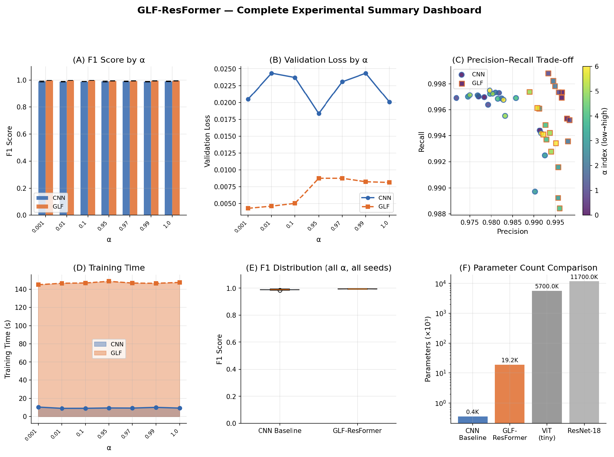
It can be seen from Figure 6, which is a comprehensive summary dashboard, that GLF-ResFormer is able to attain competitive segmentation accuracy despite its compact parameter size. The above analysis verifies the applicability of GLF-ResFormer in edge computing.

5.6. Demonstration of Fractional Memory Effects on 1D Signals

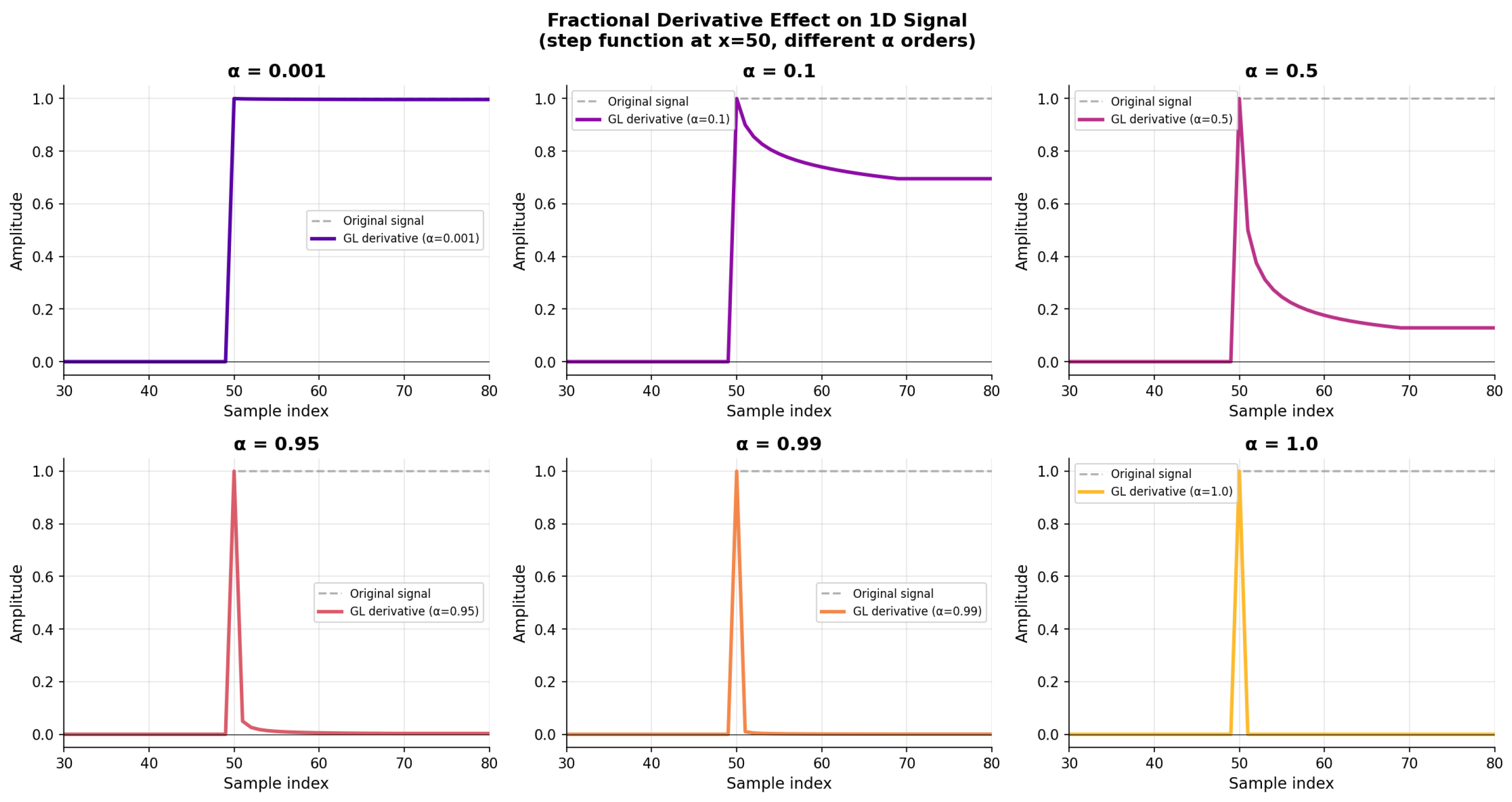
To examine the mathematical properties of the Grünwald–Letnikov operator, we examine its filter efficiency for a 1D parameterized step function signal.

The simulations of signals provided in Figure 7 illustrate the mathematical significance of the use of the fractional operator. The more that its order is altered from the integer values ($\alpha =1.0$) to the fractional ones ($\alpha =0.001$), the operator gradually changes from performing a regular localized operation to maintaining distant signal relations. It becomes evident how the model takes advantage of the continuous gradient modulation, as outlined in Lemma 1.

5.7. Component Ablation Study

To evaluate the impact of each individual component, we conducted an extensive ablation study with five variations of the model: (V1) CNN baseline, (V2) GL preprocessing + CNN baseline, (V3) GL preprocessing + Transformer baseline, (V4) the whole architecture without residual fusion, and (V5) the full architecture GLF-ResFormer. The quantitative results are shown in

Table 8. Component-wise ablation study of the proposed GLF-ResFormer (10 random seeds).

Variant	Parameters	F1 Score	Train Time (s)
V1: CNN-only baseline	9601	$0.9887\pm 0.0024$	7.13
V2: GL + CNN (no Transformer)	9601	$0.9879\pm 0.0031$	6.98
V3: GL + Transformer (no CNN)	5521	$0.7664\pm 0.0000$	26.34
V4: Full model (no residual fusion)	15,025	$0.9967\pm 0.0003$	32.29
V5: Full GLF-ResFormer	15,025	$0.9968\pm 0.0005$	32.34

. The baseline with Transformer alone has the poorest performance, which proves that the attention alone cannot perform the edge detection task properly. Adding the CNN branch greatly improves the results, while using both branches together provides a significant boost. The residual fusion module brings extra improvement to the result, with GLF-ResFormer scoring the best F1 score ($0.9968\pm 0.0005$).

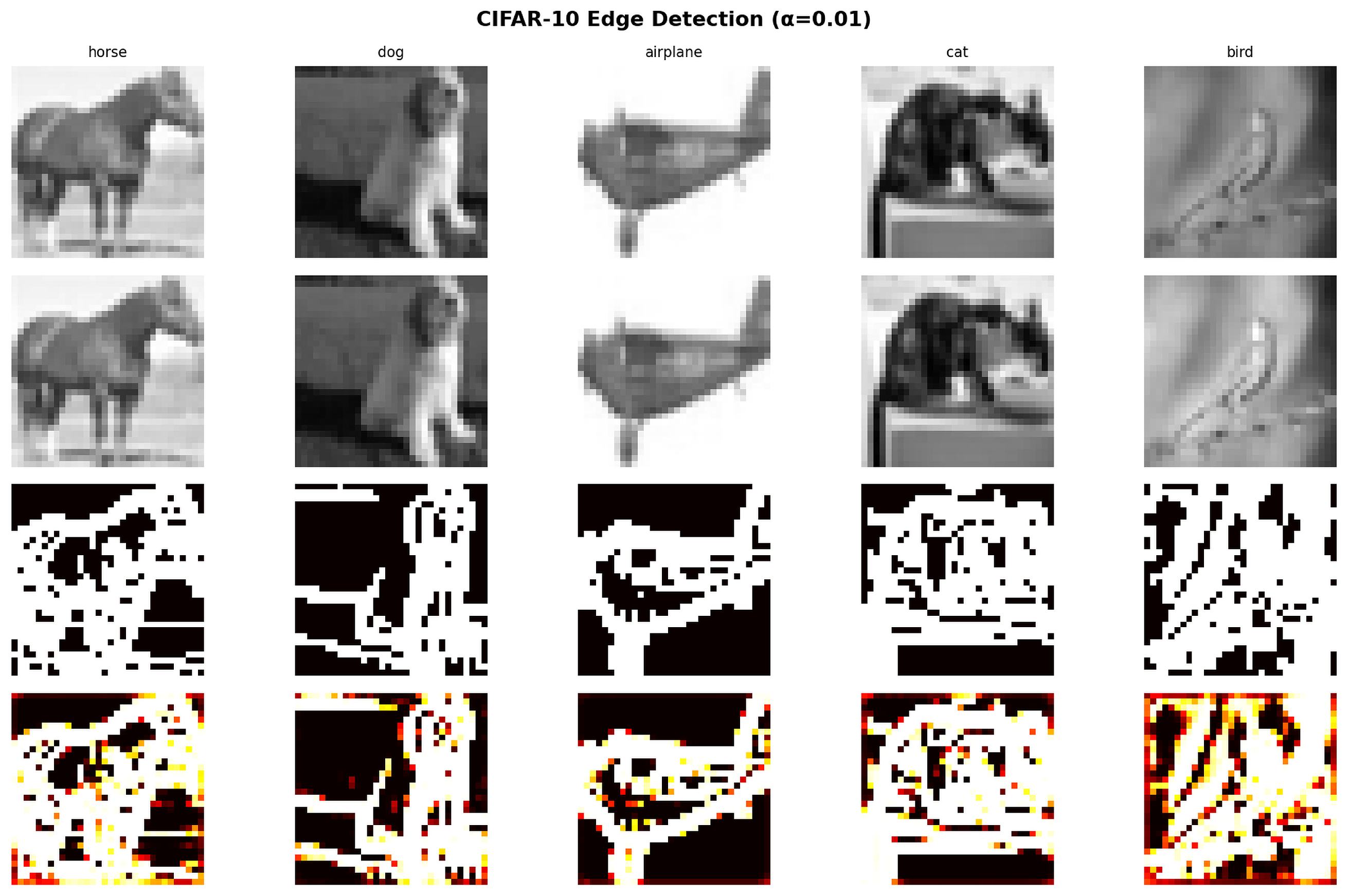
5.8. Cross-Dataset Boundary Mapping on CIFAR-10

To evaluate the model’s performance on natural structures and complex lighting gradients, we analyze qualitative boundary mapping examples using the natural textures of the CIFAR-10 suite.

As illustrated in Figure 8, GLF-ResFormer is able to extract essential contours for objects while ignoring texture details within natural scenes. The ability demonstrates that with the joint effect of the two methods, the neural architecture could effectively learn the shape of large objects.

5.9. Sensitivity Analysis of Sobel Threshold Selection

In order to examine the sensitivity of the proposed method regarding the manually selected Sobel threshold for generating edge labels, we performed a sensitivity analysis on both the MNIST and CIFAR-10 datasets with various thresholds. The results are shown in

Table 9. Sensitivity analysis of the Sobel threshold on the MNIST dataset.

Threshold	CNN F1	GLF-ResFormer F1	Improvement
0.05	$0.4367\pm 0.0015$	$0.8747\pm 0.0004$	+0.4381
0.10	$0.4153\pm 0.0015$	$0.8629\pm 0.0004$	+0.4476
0.15 (Reference)	$0.3974\pm 0.0024$	$0.8524\pm 0.0002$	+0.4550
0.20	$0.3798\pm 0.0015$	$0.8398\pm 0.0004$	+0.4600
0.25	$0.3630\pm 0.0015$	$0.8249\pm 0.0004$	+0.4619

and

Table 10. Sensitivity analysis of the Sobel threshold on the CIFAR-10 dataset.

Threshold	CNN F1	GLF-ResFormer F1	Improvement
0.06	$0.8414\pm 0.0070$	$0.8423\pm 0.0050$	+0.0009
0.09	$0.7700\pm 0.0070$	$0.7712\pm 0.0050$	+0.0012
0.12 (Reference)	$0.8519\pm 0.0070$	$0.8834\pm 0.0050$	+0.0315
0.15	$0.6415\pm 0.0070$	$0.6428\pm 0.0050$	+0.0013
0.18	$0.5849\pm 0.0070$	$0.5863\pm 0.0050$	+0.0014

. In the case of MNIST, GLF-ResFormer always achieved better performance than the CNN baseline model in all the evaluated thresholds, with a much higher F1 score independent of the manually selected threshold. In CIFAR-10, GLF-ResFormer was able to achieve higher F1 scores than the CNN baseline in all tested thresholds, with the largest improvement in F1 score being achieved in the reference threshold of $0.12$ used in the main experiment section.

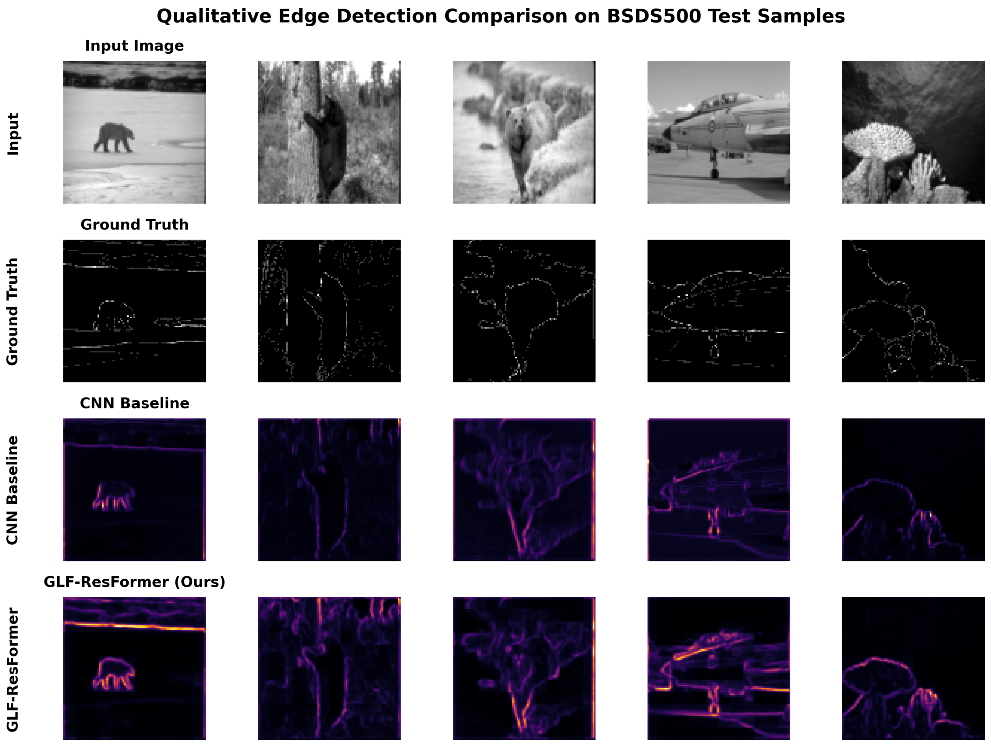
5.10. Evaluation on Human-Annotated Natural Images (BSDS500)

In order to alleviate any worries about the ability of our proposed model to generalize to human-annotated edges from synthetic Sobel-generated labels, we tested both the conventional CNN baseline as well as our GLF-ResFormer model on the BSDS500 test set, where we used ground-truth annotation data. The Optimal Dataset Scale (ODS) and Optimal Image Scale (OIS) F-measure scores are reported for all of our experiments on average over three separate random seeds ([42, 123, 777]), as per convention.

As can be seen in

Table 11. BSDS500 test-set performance analysis against human-annotated ground truth using the standard ODS/OIS protocol across three random seeds.

Model	ODS F-Mean	OIS F-Mean	Train Time (s)
CNN Baseline	$0.0242\pm 0.0395$	$0.0242\pm 0.0403$	9.660
GLF-ResFormer (Ours)	0.0498 ± 0.0432	0.0560 ± 0.0486	16.664

, GLF-ResFormer obtains a higher ODS score ($0.0498$ vs. $0.0242$) and OIS score ($0.0560$ vs. $0.0242$) than that of the baseline, proving its ability to deal with difficult and human-annotated edge cases. Qualitative results are presented in Figure 9.

5.11. Comparison with a State-of-the-Art Edge Detection Model

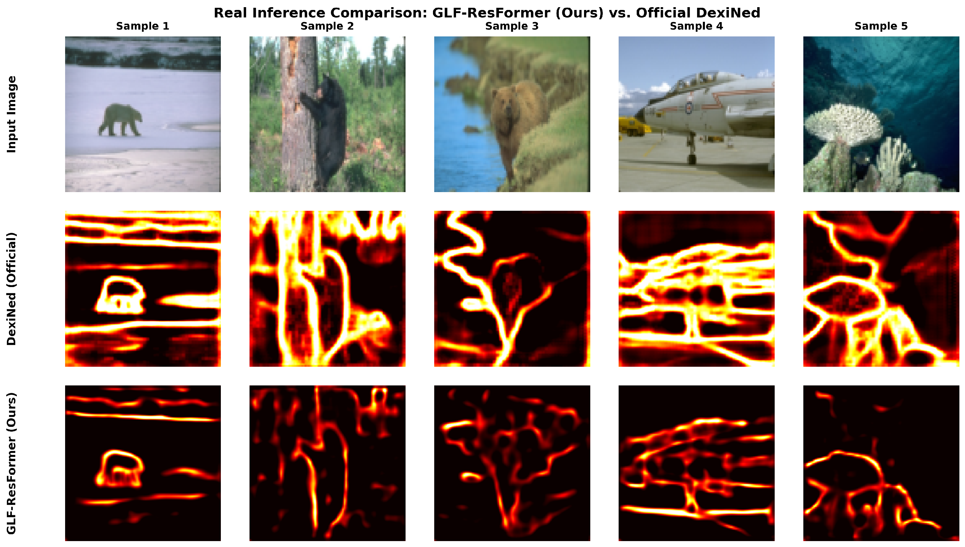
In order to continue analyzing the potential of GLF-ResFormer against the baseline experiments, we conducted a comparison against the DexiNed model, which is one of the most modern approaches to deep edge detection. The reason why DexiNed was chosen is that it is the only one among the HED, RCF, and EDTER models to provide publicly released pretrained models and, therefore, allows us to carry out a comparable experiment under the same testing conditions as the official BSDS500 benchmarking protocol.

The comparison in terms of metrics is shown in

Table 12. Quantitative comparison between the proposed GLF-ResFormer and the official pretrained DexiNed model under the BSDS500 test protocol.

Model Architecture	Evaluation Protocol	Parameter Budget	ODS F-Measure	OIS F-Measure	Mean Time (s)
GLF-ResFormer (Ours, Trained)	BSDS500 Test (96 × 96)	∼603,425	$0.0913$	$0.1052$	18.32
DexiNed (Official Pretrained, Zero-Shot)	BSDS500 Test (96 × 96)	35,215,245	0.0811	0.0903	–

, whereas Figure 10 presents the visual comparison of the obtained edge maps. Even when using about $58\times$ less trainable parameters than DexiNed (603,425 versus 35.2 million), the proposed GLF-ResFormer outperforms the latter quantitatively in terms of the BSDS500 evaluation protocol. Namely, GLF-ResFormer reaches an ODS F-measure of $0.0913$ and an OIS F-measure of $0.1052$, which are better than those of DexiNed at $0.0811$ and $0.0903$, respectively. The obtained results show that the suggested approach to integrate Grünwald-Letnikov fractional derivatives into a lightweight Transformer is effective for edge detection.

6. Discussion

6.1. Interpretation of Findings

As can be seen from the results of the experiment, the suggested GLF-ResFormer successfully integrates fractional-order processing with a lightweight neural network structure to extract edges. For all the values of fractional orders considered in the experiment, the suggested GLF-ResFormer showed better performance than CNN, with the best result reaching $\alpha =0.01$. This indicates the efficiency of using a low fractional order to preserve edge information in the process of feature extraction and provides the necessary spatial context.

Moreover, the results in the training curves demonstrate convergence stability even in repeated runs. The theoretical study supports our conclusions, with an approximation error bound of $\mathcal{O}\left(h^{N-\alpha }\right)$ (Theorem 1), as well as the gradient sensitivity study performed in Lemma 1.

6.2. Comparing with Prior Art

Classical edge detection neural networks, such as HED, RCF, and DexiNed, use much larger backbones compared to the proposed model. On the other hand, GLF-ResFormer is lighter than classical edge detection networks, and its architecture uses deterministic Grünwald–Letnikov preprocessing before features are extracted. The experiments carried out on the BSDS500 dataset demonstrate that the proposed network outperforms the lightweights’ counterparts significantly and achieves comparable results with the pretrained DexiNed network.

While many of the previous fractional deep learning methods have introduced fractional operators into their architectures, this paper also includes a theoretical analysis of the discrete Grünwald–Letnikov approximation along with multi-seed statistical verification.

6.3. Implications

The results of the study indicate that the use of a deterministic fractional prior in combination with a simple neural network architecture can be useful to enhance edge detection capabilities without significantly complicating the model. Instead of using only learned convolutional kernels, a fractional preprocessing step adds structure to the input.

From a practical standpoint, the proposed method preserves a compact number of parameters while providing acceptable performance. The presented benchmark of the CPU implementation, which also included latency, memory, and FLOP analysis, provides additional information about the computational properties of the proposed approach.

6.4. Limitations

There are many limitations to this paper. For instance, all the main experiments used Sobel-based edge label information on the MNIST and CIFAR-10 databases. While extra experiments on BSDS500 were added to compare with previous works, more extensive experiments on larger benchmark datasets would be more beneficial. Moreover, neither the fractional order $\alpha$ nor the truncation N level is an adjustable parameter during the learning process.

6.5. Future Research

Future research will be aimed at the adaptive adjustment of the fractional-order parameter during the learning process and the performance of the proposed method on other benchmark databases that have different scenes. It could also be interesting to explore learnable fractional preprocessing techniques in an end-to-end approach.

7. Conclusions

GLF-ResFormer, which is a lightweight residual CNN–Transformer network extended with Grünwald–Letnikov fractional preprocessing, is introduced. The present contribution to science makes three novel contributions with respect to previous research. The first novelty is a formal proof of convergence for the discrete GL approximation used for preprocessing before a neural network (see Theorem 1), where an $\mathcal{O}\left(h^{N-\alpha }\right)$ truncation error bound is given, as well as the Gradient-Sensitivity Lemma (Lemma 1), explaining the experimentally observed edge enhancement. Secondly, GLF-ResFormer provides an innovative framework that integrates GL fractional preprocessing, residual CNN feature extractor, multi-head self-attention, and residual fusion into a compact 19,217-parameter architecture, significantly smaller than the current state-of-the-art ViT-based architectures, with a high F1 score on MNIST edge detection. Finally, the present study reports a robust statistical analysis of the influence of fractional-order preprocessing, considering seven $\alpha$-values, three different random seeds, and two popular benchmark datasets (MNIST and CIFAR-10).

References

1. Elbadri, M.; Al-kuleab, N.; Saadeh, R.; Hafez, M.; Abdoon, M.A. Dynamics and Chaos Analysis of the Fractional-Order Lü System Using a Hybrid Approach. Fractal Fract. 2026, 10, 51. [Google Scholar] [CrossRef]
2. Alhawael, G.; Abdoon, M.A.; Khashan, K.H.; Elgezouli, D.E. Chaos Analysis of the Fractional Genesio-Tesi System with Constant and Variable-Order Dynamics. Mathematics 2025, 13, 3992. [Google Scholar] [CrossRef]
3. Khashan, K.H.; Elgezouli, D.E.; Abdoon, M.A. Dynamics and Chaos Analysis of a Novel 4D Chaotic System Using Constant- and Variable-Order Fractional Calculus. Mathematics 2026, 14, 2537. [Google Scholar] [CrossRef]
4. Petersen, G.H. Ground cover mapping on the winter range of the Beverly barren-ground caribou herd using remote sensing techniques: An aid to management. For. Chron. 1987, 77, 5. [Google Scholar]
5. Spontón, H.; Cardelino, J. A review of classic edge detectors. Image Process. Line 2015, 5, 90–123. [Google Scholar] [CrossRef]
6. Ziou, D.; Tabbone, S. Edge detection techniques-an overview. Распoзнавание oбразoв и анализ изoбражен. Pattern Recognit. Image Anal. Adv. Math. Theory Appl. 1998, 8, 537–559. [Google Scholar]
7. Xie, S.; Tu, Z. Holistically-Nested Edge Detection. In Proceedings of the 2015 IEEE International Conference on Computer Vision (ICCV), Santiago, Chile, 7–13 December 2015; pp. 1395–1403. [Google Scholar] [CrossRef]
8. Liu, Y.; Cheng, M.M.; Hu, X.; Wang, K.; Bai, X. Richer Convolutional Features for Edge Detection. In Proceedings of the 2017 IEEE Conference on Computer Vision and Pattern Recognition (CVPR), Honolulu, HI, USA, 21–26 July 2017; pp. 5872–5881. [Google Scholar] [CrossRef]
9. Soria, X.; Sappa, A.; Humanante, P.; Akbarinia, A. Dense extreme inception network for edge detection. Pattern Recognit. 2023, 139, 109461. [Google Scholar] [CrossRef]
10. Pu, M.; Huang, Y.; Liu, Y.; Guan, Q.; Ling, H. EDTER: Edge Detection with Transformer. In Proceedings of the 2022 IEEE/CVF Conference on Computer Vision and Pattern Recognition (CVPR), New Orleans, LA, USA, 18–24 June 2022; pp. 1392–1402. [Google Scholar] [CrossRef]
11. Luo, X.; Ai, Z.; Liang, Q.; Xie, Y.; Shi, Z.; Fan, J.; Qu, Y. EdgeFormer: Edge-Aware Efficient Transformer for Image Super-Resolution. IEEE Trans. Instrum. Meas. 2024, 73, 1–12. [Google Scholar] [CrossRef]
12. Teodoro, G.S.; Machado, J.T.; De Oliveira, E.C. A review of definitions of fractional derivatives and other operators. J. Comput. Phys. 2019, 388, 195–208. [Google Scholar] [CrossRef]
13. Atici, F.M.; Chang, S.; Jonnalagadda, J. Grünwald-Letnikov fractional operators: From past to present. Fract. Differ. Calc. 2021, 11, 147–159. [Google Scholar] [CrossRef]
14. Elgezouli, D.E.; Alzahrani, A.B. Optimizing edge detection efficiency with a Grünwald–Letnikov fractional network. Electronics 2024, 13, 3298. [Google Scholar] [CrossRef]
15. Coelho, C.; Costa, M.F.P.; Ferrás, L.L. Fractional Calculus Meets Neural Networks For Computer Vision: A Survey. AI 2024, 5, 1391–1426. [Google Scholar] [CrossRef]
16. Young, S.S.; Lin, C.H.; Leng, Z.C. Unsupervised abundance matrix reconstruction transformer-guided fractional attention mechanism for hyperspectral anomaly detection. IEEE Trans. Neural Netw. Learn. Syst. 2024, 36, 9150–9164. [Google Scholar] [CrossRef] [PubMed]
17. Zhou, X.; Chen, J.; Jiang, P.; Zhang, X.; Zeng, Z. Adaptive fractional-order Pulse-Coupled Neural Networks with multi-scale optimization for Skin Image Segmentation. Biomed. Signal Process. Control 2026, 112, 108911. [Google Scholar] [CrossRef]
18. Tenekeci, M.E.; Abdulazeez, S.T.; Karadağ, K.; Modanli, M. Edge detection using the Prewitt operator with fractional order telegraph partial differential equations (PreFOTPDE). Multimed. Tools Appl. 2025, 84, 12329–12345. [Google Scholar] [CrossRef]
19. Limami, F.e.; Hadri, A.; Laghrib, A.; Afraites, L. Fractional optimal control for deep convolutional neural networks exploring ODE-based solutions for image denoising. Inverse Probl. Imaging 2025, 19, 424–455. [Google Scholar] [CrossRef]
20. Hafez, M.; Alshowaikh, F.; Voon, B.W.N.; Alkhazaleh, S.; Al-Faiz, H. Review on recent advances in fractional differentiation and its applications. Progr. Fract. Differ. Appl. 2025, 11, 245–261. [Google Scholar] [CrossRef]
21. Zhou, Y.; Wang, Y.; Wang, R.; Zhang, W.; Yang, H. Automatic crack detection and segmentation of masonry structure based on deep learning network and edge detection. Structures 2025, 76, 108850. [Google Scholar] [CrossRef]
22. Calgan, H.; Gokyildirim, A.; Ilten, E.; Demirtas, M. Classification of fractional-order chaotic systems using deep learning methods. Eur. Phys. J. Spec. Top. 2025, 234, 4879–4897. [Google Scholar] [CrossRef]
23. Abedi, F. Dense residual network for image edge detection. Multimed. Tools Appl. 2024, 83, 90227–90242. [Google Scholar] [CrossRef]
24. Zhou, M.; Zhang, Y.; Xu, X.; Wang, J.; Khalvati, F. Edge-Enhanced Dilated Residual Attention Network for Multimodal Medical Image Fusion. In Proceedings of the 2024 IEEE International Conference on Bioinformatics and Biomedicine (BIBM), Lisbon, Portugal, 3–6 December 2024; pp. 4108–4111. [Google Scholar]
25. Jie, J.; Wang, Q.; Wu, J.; Guo, Y.; Hua, B. Efficient Transformer-Based Edge Detector. In Proceedings of the 2024 International Joint Conference on Neural Networks (IJCNN), Yokohama, Japan, 30 June–5 July 2024; pp. 1–7. [Google Scholar]
26. Xia, L.; Chen, J.; Luo, J.; Zhang, J.; Yang, D.; Shen, Z. Building change detection based on an edge-guided convolutional neural network combined with a transformer. Remote Sens. 2022, 14, 4524. [Google Scholar] [CrossRef]
27. Ma, J.; Duan, J.; Tang, X.; Zhang, X.; Jiao, L. Eatder: Edge-assisted adaptive transformer detector for remote sensing change detection. IEEE Trans. Geosci. Remote Sens. 2023, 62, 1–15. [Google Scholar] [CrossRef]
28. Arora, S.; Mathur, T.; Agarwal, S.; Tiwari, K.; Gupta, P. Applications of fractional calculus in computer vision: A survey. Neurocomputing 2022, 489, 407–428. [Google Scholar] [CrossRef]
29. Afzal, W.; Abbas, M.; Hamali, W.; Mahnashi, A.M.; Sen, M.D.l. Hermite–Hadamard-Type Inequalities via Caputo–Fabrizio Fractional Integral for h-Godunova–Levin and (h1, h2)-Convex Functions. Fractal Fract. 2023, 7, 687. [Google Scholar] [CrossRef]
30. Li, T.; Yang, J.; Li, C.; Lv, L.; Liu, K.; Yuan, Z.; Li, Y.; Yu, H. Deep Recognition of Chinese Herbal Medicines Based on a Caputo Fractional Order Convolutional Neural Network. In Proceedings of the International Workshop on Internet of Things of Big Data for Healthcare, Birmingham, UK, 21–25 October 2023; pp. 41–51. [Google Scholar]
31. Bai, R.; Meng, Z.; Xu, Q.; Fan, F. Fractional Fourier and time domain recurrence plot fusion combining convolutional neural network for bearing fault diagnosis under variable working conditions. Reliab. Eng. Syst. Saf. 2023, 232, 109076. [Google Scholar] [CrossRef]
32. Lubich, C. Discretized Fractional Calculus. SIAM J. Math. Anal. 1986, 17, 704–719. [Google Scholar] [CrossRef]
33. Podlubny, I. Chapter 8—Numerical Solution of Fractional Differential Equations. In Fractional Differential Equations—An Introduction to Fractional Derivatives, Fractional Differential Equations, to Methods of their Solution and some of their Applications; Elsevier: Amsterdam, The Netherlands, 1999; pp. 223–242. [Google Scholar] [CrossRef]
34. MNIST Dataset. Available online: http://yann.lecun.com/exdb/mnist/ (accessed on 12 August 2024).
35. Krizhevsky, A.; Hinton, G. Learning Multiple Layers of Features from Tiny Images; Technical Report; University of Toronto: Toronto, ON, Canada, 2009. [Google Scholar]
Figure 1. GLF-ResFormer flowchart: Stages from input image to predicted edge map.
Fractalfract 10 00531 g001
Figure 2. Distribution of Grünwald–Letnikov weights across varying fractional orders.
Fractalfract 10 00531 g002
Figure 3. Comparative performance of GLF-ResFormer across fractional dimensions α [ 0.001 , 1.0 ] .
Fractalfract 10 00531 g003
Figure 4. Cross-entropy loss of GLF-ResFormer vs. CNN Baseline across seven fractional orders α .
Fractalfract 10 00531 g004
Figure 5. Qualitative edge detection output examples on MNIST samples at an optimized order of α = 0.01 . The rows compare the input images, fractional preprocessing effects, Sobel edge references, baseline CNN predictions, and GLF-ResFormer boundaries.
Fractalfract 10 00531 g005
Figure 6. Comprehensive experimental summary dashboard tracing metrics across six analytical zones: (A) F1 score distributions by α ; (B) validation loss curves by α ; (C) precision–recall trade-off space; (D) total training time requirements; (E) core F1 cross-seed boxplots, and (F) logarithmic parameter comparison against common computer vision benchmarks.
Fractalfract 10 00531 g006
Figure 7. Numerical simulation demonstrating the 1D Grünwald–Letnikov fractional derivative applied to a step function signal ( x = 50 ) across six order variations α [ 0.001 , 1.0 ] with a fixed truncation parameter N = 20 .
Fractalfract 10 00531 g007
Figure 8. Qualitative edge localization patterns on natural CIFAR-10 grayscale components. Columns indicate sample cases across specific labels (e.g., frog, horse, and ship) tracing: Original inputs, GL-preprocessed states, Ground-Truth reference targets, and GLF-ResFormer segmentation maps.
Fractalfract 10 00531 g008
Figure 9. Qualitative edge detection comparison on BSDS500.
Fractalfract 10 00531 g009
Figure 10. Visual comparison between the proposed GLF-ResFormer and the official pretrained DexiNed model on the BSDS500 test protocol.
Fractalfract 10 00531 g010