Existence, Uniqueness, and Continuous Dependence on Initial/Final Values for Liouville–Caputo Fractional Difference Equations

Abstract

This paper develops a unified qualitative framework for four classes of Liouville–Caputo fractional difference equations arising from different combinations of fractional sums and integer-order differences. Based on the equivalence between initial/final value problems and Volterra-type summation equations, sufficient conditions for the existence and uniqueness of solutions are established by applying the Banach contraction mapping principle together with refined combinatorial estimates. Furthermore, the continuous dependence of solutions on prescribed initial or final data is investigated. By deriving explicit error estimates through a discrete fractional Gronwall-type inequality, we prove that Lipschitz solutions depend continuously on perturbations of boundary data. Numerical experiments for a representative case are presented to verify the theoretical results, including the influence of the fractional order and the sensitivity with respect to boundary data, while additional examples illustrate the applicability of the framework. The obtained results extend the unified discrete fractional calculus framework by providing a rigorous well-posedness analysis and offering a theoretical foundation for further applications of discrete fractional models with memory effects and diverse boundary conditions.

1. Introduction

Fractional calculus has become an important framework in modern applied mathematics due to its capability of describing memory and hereditary properties in complex systems. Since the introduction of the Liouville–Caputo fractional derivative [1], fractional-order models have attracted extensive attention and have been successfully applied in various areas, including memristive circuits [2], infectious disease modeling [3], control theory [4,5], and economic dynamics [6]. Meanwhile, difference equations have played a fundamental role in the analysis and modeling of discrete-time systems, with classical contributions in stability theory [7,8] and systematic treatments provided in the monographs of Kocic and Ladas [9] and Agarwal [10]. Comprehensive introductions to fractional calculus and fractional differential equations can be found in the classical monographs by Oldham and Spanier [11], Kilbas et al. [12], and Podlubny [13].

The combination of fractional calculus and discrete analysis has led to the rapid development of discrete fractional calculus. Several discrete fractional operators, including the Grünwald–Letnikov [14], Riemann–Liouville [15], and Liouville–Caputo [16] formulations, have been introduced. Among them, Goodrich and Peterson [17] provided a systematic foundation for discrete fractional calculus, particularly emphasizing forward fractional differences. Subsequently, different qualitative and numerical aspects of discrete fractional equations have been investigated. For instance, Laledj et al. [18] studied implicit fractional q-difference equations using fixed-point methods, while Allouch et al. [19] and Alili et al. [20] considered boundary value problems and fractional difference inclusion problems, respectively. Hattaf [21] further investigated numerical schemes for nonlinear fractional models.

A Liouville–Caputo fractional difference operator can be interpreted as the composition of a fractional sum and an integer-order difference operator. Since fractional sums can be defined through variable upper-limit and variable lower-limit formulations, while integer-order differences can be constructed in forward and backward directions, four distinct Liouville–Caputo fractional difference formulations naturally arise. However, these four formulations have not yet been systematically studied within a unified theoretical framework. Early developments of discrete fractional calculus mainly focused on the variable upper-limit fractional sum combined with the forward difference operator [17]. Cheng and Chu [22] considered a formulation involving the variable upper-limit fractional sum and the backward difference operator, but a general framework covering all combinations of fractional sums and difference directions was not established.

To overcome this limitation, our previous work [23] developed a unified framework for the four Liouville-Caputo fractional difference formulations with variable bounds. In that work, the four definitions were introduced, their fundamental properties were established, their equivalence with corresponding Volterra-type summation equations was proved, and explicit solution representations were obtained. These results provide the necessary analytical foundation for further investigation of the qualitative properties of the corresponding solutions. However, the existence, uniqueness, and continuous dependence of solutions, which are essential aspects of well-posedness, remain open problems.

In the continuous setting, the qualitative analysis of fractional equations, especially existence and uniqueness theory, has been extensively investigated. Various techniques have been developed for different classes of fractional differential equations. For example, Salem and Mshary [24] studied fractional Langevin equations, Nanware and Dhaigude [25] considered fractional equations with integral boundary conditions, Ahmad and Alsaedi [26] investigated coupled fractional systems, and Ardjouni and Djoudi [27] established results for nonlinear Liouville–Caputo fractional differential equations. More recently, Baroudi et al. [28], Benzenati et al. [29], Azzouz and Beddani [30], Promsakon et al. [31], Graef et al. [32], and Ezugorie et al. [33] extended existence, uniqueness, and stability analyses to various fractional models. Of particular relevance to the present work, Islam et al. [34] investigated Caputo fractional differential equations by transforming the problems into equivalent Volterra integral equations and applying contraction arguments. Their work also highlighted the potential extension of such qualitative analysis to discrete fractional calculus. Motivated by these developments, this paper establishes a unified well-posedness theory for the four Liouville–Caputo fractional difference formulations introduced in [23]. By utilizing the equivalent Volterra-type summation equations, each initial/final value problem is reformulated as a fixed-point problem in a Banach space. The Banach contraction mapping principle is then applied to derive sufficient conditions for the existence and uniqueness of solutions. Furthermore, the continuous dependence of solutions on initial/final data is established through explicit Lipschitz-type estimates obtained from a discrete fractional Gronwall-type inequality. Compared with [23], which focused on the construction of the operators and the representation of solutions, the present work investigates their qualitative properties and completes an essential part of the unified discrete fractional calculus framework. Numerical examples are also provided to illustrate and validate the theoretical results. The remainder of this paper is organized as follows. Section 2 introduces preliminary definitions and auxiliary results. Section 3 presents the main theoretical results on existence, uniqueness, and continuous dependence. Section 4 provides numerical examples, and Section 5 concludes the paper.

2. Preliminaries

In this section, we will introduce fundamental concepts essential for the remainder of the paper. These include the Gamma function, fractional order difference and sum, initial and terminal value problems of solutions, as well as contraction mapping and the fixed point theorem. Familiarizing oneself with these preliminaries will provide a solid basis for understanding the subsequent discussions and methodologies. At the end of this section, we also provide a brief comparison between the present work and our companion paper [23] to clarify the distinct contributions of each study.

2.1. Basic Definitions and Tools

Definition 1

([23]). Let $x\in {\mathbb{R}}_{+}$, and the Gamma function is defined as

$$\Gamma \left(x\right)={\int }_0^{+\infty }{e}^{-t}{t}^{x-1}dt,$$

(1)

with the convention that $0!=1$. It possesses the following properties:

1. 

$\Gamma (x+1)=x\Gamma \left(x\right)$,

2. 

$\Gamma \left(n\right)=(n-1)!$, where $n\in {\mathbb{N}}_{+}$.

Definition 2

([23]). Let $x,\alpha \in {\mathbb{R}}_{+}$, and the fractional factorial is defined as

$$x^{\overline{\alpha }}={\displaystyle \frac{\Gamma (x+\alpha )}{\Gamma \left(x\right)}},x^{\underline{\alpha }}={\displaystyle \frac{\Gamma (x+1)}{\Gamma (x-\alpha +1)}}.$$

(2)

Definition 3

([23], Fractional forward variable upper limit sum). Let $a\in \mathbb{Z}$ be a constant, $n\in {\mathbb{Z}}_a$ and $\alpha \in {\mathbb{R}}^{+}$, we call

$${}_a{}^{ }\Delta _{ }^{-\alpha }x\left(n\right)={\displaystyle \frac{1}{\Gamma \left(\alpha \right)}}{\displaystyle \sum _{i=a}^{n-\alpha }}{(n-i-1)}^{\underline{\alpha -1}}x\left(i\right)={\displaystyle \frac{1}{\Gamma \left(\alpha \right)}}{\displaystyle \sum _{i=a}^{n-\alpha }}{\displaystyle \frac{\Gamma (n-i)}{\Gamma (n-i-\alpha +1)}}x\left(i\right)$$

(3)

the α-order forward variable upper limit sum of $x\left(n\right)$.

Here, ${\mathbb{Z}}_a=\{a+1,a+2,\dots \}$.

Definition 4

([23], Fractional forward variable lower limit sum). Let $b\in \mathbb{Z}$ be a constant, $n\in {\mathbb{Z}}_{-\infty ,b}$ and $\alpha \in {\mathbb{R}}^{+}$, we call

$${\mathsf{\nabla }}_b^{-\alpha }x\left(n\right)={\displaystyle \frac{1}{\Gamma \left(\alpha \right)}}{\displaystyle \sum _{i=n}^{b-1}}{(i-n+1)}^{\overline{\alpha -1}}x\left(i\right)={\displaystyle \frac{1}{\Gamma \left(\alpha \right)}}{\displaystyle \sum _{i=n}^{b-1}}{\displaystyle \frac{\Gamma (i-n+\alpha )}{\Gamma (i-n+1)}}x\left(i\right)$$

(4)

the α-order forward variable lower limit sum of $x\left(n\right)$.

Here, ${\mathbb{Z}}_{-\infty ,b}=\{\dots ,b-2,b-1\}$.

Definition 5

([23], Fractional backward variable upper limit sum). Let $a\in \mathbb{Z}$ be a constant, $n\in {\mathbb{Z}}_a$ and $\alpha \in {\mathbb{R}}^{+}$, we call

$${}_a{}^{ }\mathsf{\nabla }_{ }^{-\alpha }x\left(n\right)={\displaystyle \frac{1}{\Gamma \left(\alpha \right)}}{\displaystyle \sum _{i=a+1}^n}{(n-i+1)}^{\overline{\alpha -1}}x\left(i\right)={\displaystyle \frac{1}{\Gamma \left(\alpha \right)}}{\displaystyle \sum _{i=a+1}^n}{\displaystyle \frac{\Gamma (n-i+\alpha )}{\Gamma (n-i+1)}}x\left(i\right)$$

(5)

the α-order backward variable upper limit sum of $x\left(n\right)$.

Definition 6

([23], Fractional backward variable lower limit sum). Let $b\in \mathbb{Z}$ be a constant, $n\in {\mathbb{Z}}_{-\infty ,b}$ and $\alpha \in {\mathbb{R}}^{+}$, we call

$${\mathsf{\nabla }}_b^{-\alpha }x\left(n\right)={\displaystyle \frac{1}{\Gamma \left(\alpha \right)}}{\displaystyle \sum _{i=n+\alpha }^b}{(i-n-1)}^{\underline{\alpha -1}}x\left(i\right)={\displaystyle \frac{1}{\Gamma \left(\alpha \right)}}{\displaystyle \sum _{i=n+\alpha }^b}{\displaystyle \frac{\Gamma (i-n)}{\Gamma (i-n-\alpha +1)}}x\left(i\right)$$

(6)

the α-order backward variable lower limit sum of $x\left(n\right)$.

To clarify the notation introduced in Definitions 3–6, the four fractional sum operators are summarized in

Table 1. Summary of the four fractional sum operators.

Operator	Type of Sum	Difference Direction	Domain of n	Summation Range	Associated Problem
${}_a{}^{ }\Delta _{ }^{-\alpha }$	Variable upper-limit	Forward ($\Delta$)	${\mathbb{Z}}_a$	$i=a$ to $n-\alpha$	Initial value
${\Delta }_b^{-\alpha }$	Variable lower-limit	Forward ($\Delta$)	${\mathbb{Z}}_{-\infty ,b}$	$i=n$ to $b-1$	Final value
${}_a{}^{ }\mathsf{\nabla }_{ }^{-\alpha }$	Variable upper-limit	Backward (∇)	${\mathbb{Z}}_a$	$i=a+1$ to n	Initial value
${\mathsf{\nabla }}_b^{-\alpha }$	Variable lower-limit	Backward (∇)	${\mathbb{Z}}_{-\infty ,b}$	$i=n+\alpha$ to b	Final value

. The table presents the summation type (variable upper-limit or variable lower-limit), the corresponding difference operator (forward difference $\Delta$ or backward difference ∇), the domain of n, the explicit summation range, and the associated initial or final value problem. This table provides a concise reference for the operators used in the subsequent sections.

Definition 7

([23], Fractional difference). Let $n\in \mathbb{Z},\alpha >0$, and assume that $m=\left[\alpha \right]+1$. Define

$${}_{ }{}^{C}D_{ }^{\alpha }x\left(n\right)=D^{-(m-\alpha )}{D}^{m}x\left(n\right)$$

(7)

as the α order Liouville–Caputo-type fractional difference, where ${}_{ }{}^{C}D_{ }^{\alpha }$ is the difference operator of order α.

Note: The superscript C stands for “Liouville–Caputo”. $[·]$ denotes rounding to the nearest integer towards zero.

Lemma 1

([23]). For any $\alpha >0,\beta \in \mathbb{R}$, it follows that

$$D^{\alpha }{D}^{\beta }=D^{\alpha +\beta }.$$

(8)

where $D^{\alpha }$ is the difference operator of order α.

Lemma 2

([23]). Let $a\in \mathbb{Z}$ be a constant, $n\in {\mathbb{Z}}_a$ and $\alpha \in {\mathbb{R}}^{+}$, $m=\left[\alpha \right]+1$. $f[n+\alpha -1,u(n+\alpha -1\left)\right]\in \mathbb{R}$ is a given function. The forward fractional difference equation is defined as

$$\left\{\begin{array}{c}{\Delta }^{\alpha }u\left(n\right)=f\left[n+\alpha -1,u(n+\alpha -1)\right],\hfill \\ {\Delta }^{k}u\left(a\right)=u_k,k=1,2,3,\cdots ,m-1.\hfill \end{array}\right.$$

(9)

The Cauchy initial value problem (Equation (9)) is equivalent to the Volterra sum equation

$$u\left(n\right)={\displaystyle \sum _{k=0}^{m-1}}{\displaystyle \frac{{(n-a)}^{\underline{k}}}{k!}}{u}_k+{\displaystyle \frac{1}{\Gamma \left(\alpha \right)}}{\displaystyle \sum _{i=a}^{n-1}}{(n-i)}^{\overline{\alpha -1}}f\left[i,u\left(i\right)\right]m=\left[\alpha \right]+1.$$

(10)

Lemma 3

([23]). Let $b\in \mathbb{Z}$ be a constant, $n\in {\mathbb{Z}}_{-\infty ,b}$ and $\alpha \in {\mathbb{R}}^{+}$, $m=\left[\alpha \right]+1$. $f[n,u(n\left)\right]\in \mathbb{R}$ is a given function. The negative forward fractional difference equation is defined as

$$\left\{\begin{array}{c}{(-\Delta ) }^{\alpha }u\left(n\right)=f\left[n,u\left(n\right)\right],\hfill \\ {(-\Delta ) }^{k}u\left(b\right)=u_k,k=0,1,2,\cdots ,m-1.\hfill \end{array}\right.$$

(11)

The Cauchy initial value problem (Equation (11)) equivalent to the Volterra sum equation

$$u\left(n\right)={\displaystyle \sum _{k=0}^{m-1}}{\displaystyle \frac{{(b-n)}^{\overline{k}}}{k!}}{u}_k+{\displaystyle \frac{1}{\Gamma \left(\alpha \right)}}{\displaystyle \sum _{i=n}^{b-1}}{(i-n+1)}^{\overline{\alpha -1}}f\left[i,u\left(i\right)\right]m=\left[\alpha \right]+1.$$

(12)

Lemma 4

([23]). Let $a\in \mathbb{Z}$ be a constant, $n\in {\mathbb{Z}}_a$ and $\alpha \in {\mathbb{R}}^{+}$, $m=\left[\alpha \right]+1$. $f[n,u(n\left)\right]\in \mathbb{R}$ is a given function. The backward fractional difference equation is defined as

$$\left\{\begin{array}{c}{\mathsf{\nabla }}^{\alpha }u\left(n\right)=f\left[n,u\left(n\right)\right],\hfill \\ {\mathsf{\nabla }}^{k}u\left(a\right)=u_k,k=0,1,2,\cdots ,m-1.\hfill \end{array}\right.$$

(13)

The Cauchy initial value problem (Equation (13)) equivalent to the Volterra sum equation

$$u\left(n\right)={\displaystyle \sum _{k=0}^{m-1}}{\displaystyle \frac{{(n-a)}^{\overline{k}}}{k!}}{u}_k+{\displaystyle \frac{1}{\Gamma \left(\alpha \right)}}{\displaystyle \sum _{i=a+1}^n}{(n-i+1)}^{\overline{\alpha -1}}f\left[i,u\left(i\right)\right]m=\left[\alpha \right]+1.$$

(14)

Lemma 5

([23]). Let $b\in \mathbb{Z}$ be a constant, $n\in {\mathbb{Z}}_{-\infty ,b}$ and $\alpha \in {\mathbb{R}}^{+}$, $m=\left[\alpha \right]+1$. $f[n-\alpha +1,u(n-\alpha +1\left)\right]\in \mathbb{R}$ is a given function. The negative backward fractional difference equation is defined as

$$\left\{\begin{array}{c}{(-\mathsf{\nabla }) }^{\alpha }u\left(n\right)=f\left[n-\alpha +1,u(n-\alpha +1)\right],\hfill \\ {(-\mathsf{\nabla }) }^{k}u\left(b\right)=u_k,k=0,1,2,\cdots ,m-1.\hfill \end{array}\right.$$

(15)

The Cauchy final value problem (Equation (15)) equivalent to the Volterra sum equation

$$u\left(n\right)={\displaystyle \sum _{k=0}^{m-1}}{\displaystyle \frac{{(b-n)}^{\underline{k}}}{k!}}{u}_k+{\displaystyle \frac{1}{\Gamma \left(\alpha \right)}}{\displaystyle \sum _{i=n+1}^b}{(i-n)}^{\overline{\alpha -1}}f\left[i,u\left(i\right)\right]m=\left[\alpha \right]+1.$$

(16)

Lemma 6

([23]). Let $\alpha >0$ and $m,n\in \mathbb{N}$. Then, the following two equalities hold:

1. 

${\displaystyle \sum _{k=0}^n}{\displaystyle \frac{{\alpha }^{\overline{k}}}{k!}}={\displaystyle \sum _{k=0}^n}{\displaystyle \frac{\alpha (\alpha +1)\cdots (\alpha +k-1)}{k!}}={\displaystyle \frac{{(\alpha +1)}^{\overline{n}}}{n!}}$,

2. 

${\displaystyle \sum _{k=0}^n}{\displaystyle \frac{{\alpha }^{\overline{n-k}}}{(n-k)!}}{\displaystyle \frac{{(m\alpha +1)}^{\overline{k}}}{k!}}={\displaystyle \frac{{\left[\right(m+1)\alpha +1]}^{\overline{n}}}{n!}}$.

Definition 8

([26], Contraction Mapping). Let $(X,d)$ be a metric space. A mapping $T:X\to X$ is called a contraction mapping if there exists a constant $k\in [0,1)$ such that for all $x,y\in X$,

$$d\left(T\right(x),T(y\left)\right)⩽k·d(x,y).$$

(17)

The constant k is referred to as the contraction coefficient.

Lemma 7

(Banach Fixed-Point Theorem [26]). Let $(X,d)$ be a complete metric space, and let $T:X\to X$ be a contraction mapping. Then the following hold:

1. 

Existence and uniqueness: There exists a unique fixed point $x^{*}\in X$ such that $T\left(x^{*}\right)=x^{*}$;

2. 

Convergence: For any initial point $x_0\in X$, the sequence $\left\{x_n\right\}$ generated by the iteration $x_{n+1}=T\left(x_n\right)$ converges to $x^{*}$;

3. 

Error estimate: The convergence rate satisfies the following inequality:

$$d(x_n,x^{*})⩽{\displaystyle \frac{k^n}{1-k}}d(x_0,x_1),$$

(18)

where k is the contraction coefficient.

Lemma 8

(Discrete Gronwall-type inequality). Let $u\left(n\right)$ be a nonnegative sequence, and let $C,A\ge 0$, $\alpha \in (0,1]$.

1. 

(Forward form) If for a fixed interval ${(a,N]}_{\mathbb{Z}}$,

$$u\left(n\right)\le C+{\displaystyle \frac{A}{\Gamma \left(\alpha \right)}}{\displaystyle \sum _{i=a}^{n-1}}{(n-i)}^{\overline{\alpha -1}}u\left(i\right),n\in {(a,N]}_{\mathbb{Z}},$$

then there exists a constant $K_1=K_1(A,\alpha ,N-a)>0$ such that

$$u\left(n\right)\le K_{1}C,\forall n\in {(a,N]}_{\mathbb{Z}}.$$

2. 

(Backward form) If for a fixed interval ${[M,b)}_{\mathbb{Z}}$,

$$u\left(n\right)\le C+{\displaystyle \frac{A}{\Gamma \left(\alpha \right)}}{\displaystyle \sum _{i=n+1}^b}{(i-n)}^{\overline{\alpha -1}}u\left(i\right),n\in {[M,b)}_{\mathbb{Z}},$$

then there exists a constant $K_2=K_2(A,\alpha ,b-M)>0$ such that

$$u\left(n\right)\le K_{2}C,\forall n\in {[M,b)}_{\mathbb{Z}}.$$

Proof. 

Forward: Since $n\le N$, the kernel sum is bounded by

$$C_{\alpha }\left(N\right):={\displaystyle \frac{1}{\Gamma \left(\alpha \right)}}{\displaystyle \sum _{k=1}^{N-a}}{k}^{\overline{\alpha -1}}<\infty ,$$

where the finiteness follows because the sum is over a finite set. Substituting this bound into the original inequality yields

$$u\left(n\right)\le C+A{C}_{\alpha }\left(N\right){\displaystyle \sum _{i=a}^{n-1}}u\left(i\right),n\in {(a,N]}_{\mathbb{Z}}.$$

This is the classical discrete Gronwall inequality (see, e.g., Agarwal [10], Theorem 2.1.1, p. 13). Applying it gives

$$u\left(n\right)\le C{(1+A{C}_{\alpha }\left(N\right))}^{n-a}\le C{(1+A{C}_{\alpha }\left(N\right))}^{N-a}=:K_{1}C,$$

where

$$K_1=K_1(A,\alpha ,N-a):={(1+A{C}_{\alpha }\left(N\right))}^{N-a}.$$

Backward: Set $v\left(m\right):=u(b-m)$ for $m\in {(0,b-M]}_{\mathbb{Z}}$. Then, the backward inequality becomes a forward inequality for v:

$$v\left(m\right)\le C+{\displaystyle \frac{A}{\Gamma \left(\alpha \right)}}{\displaystyle \sum _{j=0}^{m-1}}{(m-j)}^{\overline{\alpha -1}}v\left(j\right),m\in {(0,b-M]}_{\mathbb{Z}}.$$

Applying the forward result just proved to v on the interval ${(0,b-M]}_{\mathbb{Z}}$, we obtain

$$v\left(m\right)\le K_{2}C,m\in {(0,b-M]}_{\mathbb{Z}},$$

with

$$K_2=K_2(A,\alpha ,b-M):={\left(1+{\displaystyle \frac{A}{\Gamma \left(\alpha \right)}}{\displaystyle \sum _{k=1}^{b-M}}{k}^{\overline{\alpha -1}}\right)}^{b-M}.$$

Since $u\left(n\right)=v(b-n)$, we have $u\left(n\right)\le K_{2}C$ for all $n\in {[M,b)}_{\mathbb{Z}}$. □

Note: The constants $K_1,K_2$ depend on the interval length, so this lemma is valid only on finite intervals and cannot be directly extended to infinite intervals. This is consistent with the finite-interval setting of the continuous dependence theorems (Theorems 5–8).

2.2. Comparison with the Previous Work [23]

Before presenting the main results, we briefly clarify the relationship between the present work and our previous study [23]. The main differences and complementary aspects of the two works are summarized in

Table 2. Comparison between the previous work [23] and the present paper.

Aspect	Li et al. [23]	Present Paper
Primary focus	Solution representations and operator framework	Qualitative properties of solutions
Main objectives	Introduction of four definitions; equivalence with Volterra sum equations; explicit solution representations	Existence, uniqueness, and Lipschitz continuous dependence on initial/final data for all four formulations
Mathematical tools	Fractional sum identities and combinatorial transformations	Banach contraction mapping principle and discrete fractional Gronwall-type inequality

.

The previous work [23] established the analytical framework and solution representations for the four Liouville–Caputo fractional difference formulations, whereas the present paper focuses on their qualitative properties, including existence, uniqueness, and continuous dependence on prescribed boundary data. Therefore, these two studies address different but complementary aspects of the unified discrete fractional calculus framework and together provide an essential theoretical foundation for further analysis.

3. Theoretical Proof and Extended Discussion on the Existence and Uniqueness of Solutions

In this section, we establish and rigorously prove four theorems concerning the existence and uniqueness of solutions for the four types of Liouville–Caputo fractional difference equations introduced in Section 2, utilizing the Banach fixed point theorem combined with refined estimates and combinatorial identities.

3.1. Theoretical Proof of the Existence and Uniqueness of Solutions

This subsection focuses on the existence and uniqueness of solutions to fractional-order difference equations under four different definitions. We propose and rigorously prove four theorems, each corresponding to one of the four definition scenarios. This not only consolidates the theoretical framework of fractional-order difference equations but also provides a basis for their practical applications, thus promoting the development of research in this field.

Theorem 1

(Forward fractional difference equation with initial value). Let $a\in \mathbb{Z}$ be a constant, and let $N\in \mathbb{Z}$ with $a<N<\infty$. Consider the initial value problem for a Liouville–Caputo fractional difference equation of order $\alpha (0<\alpha \le 1)$ on the finite interval ${(a,N]}_{\mathbb{Z}}$:

$$\left\{\begin{array}{c}{\Delta }^{\alpha }y\left(n\right)=f\left[n+\alpha -1,y(n+\alpha -1)\right],\hfill \\ y\left(a\right)=y_0,\hfill \end{array}\right.$$

(19)

where ${\Delta }^{\alpha }$ denotes the Liouville–Caputo fractional difference operator of order α, $f:{(a,N]}_{\mathbb{Z}}\times \mathbb{R}\to \mathbb{R}$ is a given function, and $y_0$ is the initial value. Assume that:

(H1) 

There exists a constant $K>0$ such that $\left|f\right(n,y\left)\right|\le K$ for all $n\in {(a,N]}_{\mathbb{Z}},y\in \mathbb{R}$;

(H2) 

f satisfies a Lipschitz condition with respect to the second variable, i.e., there exists a constant $A>0$ such that

$$|f(n,y_1)-f(n,y_2)| \le A|y_1-y_2|,\forall n\in {(a,N]}_{\mathbb{Z}},y_1,y_2\in \mathbb{R},$$

and moreover, $0<A<1$.

Then, problem (19) possesses a unique solution $y\left(n\right)$ on ${(a,N]}_{\mathbb{Z}}$.

Proof. 

By Lemma 2, the initial value problem (19) is equivalent to the Volterra sum equation

$$y\left(n\right)=y_0+{\displaystyle \frac{1}{\Gamma \left(\alpha \right)}}{\displaystyle \sum _{i=a}^{n-1}}{(n-i)}^{\overline{\alpha -1}}f\left[i,y\left(i\right)\right],n\in {(a,N]}_{\mathbb{Z}}.$$

(20)

(For $n=a$, the sum is empty and the equality reduces to $y\left(a\right)=y_0$.) This equivalence is guaranteed by the corresponding lemma in [23]. Hence, it suffices to prove that (20) admits a unique solution on ${(a,N]}_{\mathbb{Z}}$.

Existence. 

Define a sequence ${\left\{y_l\left(n\right)\right\}}_{l\ge 0}$ by

$$y_0\left(n\right)\equiv y_0,y_l\left(n\right)=y_0+{\displaystyle \frac{1}{\Gamma \left(\alpha \right)}}{\displaystyle \sum _{i=a}^{n-1}}{(n-i)}^{\overline{\alpha -1}}f\left[i,y_{l-1}\left(i\right)\right],l=1,2,\dots ,n\in {(a,N]}_{\mathbb{Z}}.$$

We first estimate the differences $|y_l\left(n\right)-y_{l-1}\left(n\right)|$. For $l=1$, using (H1) and the identity (see Lemma 6)

$${\displaystyle \frac{1}{\Gamma \left(\alpha \right)}}{\displaystyle \sum _{i=a}^{n-1}}{(n-i)}^{\overline{\alpha -1}}={\displaystyle \frac{{(\alpha +1)}^{\overline{n-a-1}}}{(n-a-1)!}},$$

we obtain, for every $n\in {(a,N]}_{\mathbb{Z}}$,

$$|y_1\left(n\right)-y_0\left(n\right)|\le {\displaystyle \frac{K}{\Gamma \left(\alpha \right)}}{\displaystyle \sum _{i=a}^{n-1}}{(n-i)}^{\overline{\alpha -1}}=K{\displaystyle \frac{{(\alpha +1)}^{\overline{n-a-1}}}{(n-a-1)!}}.$$

For $l=2$, by the Lipschitz condition (H2) and the previous estimate,

$$\begin{array}{cc}\hfill |y_2\left(n\right)-y_1\left(n\right)|& \le {\displaystyle \frac{A}{\Gamma \left(\alpha \right)}}{\displaystyle \sum _{i=a}^{n-1}}{(n-i)}^{\overline{\alpha -1}}|y_1\left(i\right)-y_0\left(i\right)|\hfill \\ & \le {\displaystyle \frac{AK}{\Gamma \left(\alpha \right)}}{\displaystyle \sum _{i=a}^{n-1}}{(n-i)}^{\overline{\alpha -1}}{\displaystyle \frac{{(\alpha +1)}^{\overline{i-a-1}}}{(i-a-1)!}}\hfill \\ & =AK{\displaystyle \frac{{(2\alpha +1)}^{\overline{n-a-1}}}{(n-a-1)!}}(\mathrm{by}\mathrm{Lemma}6).\hfill \end{array}$$

Assume inductively that for some $l\ge 2$, for all $n\in {(a,N]}_{\mathbb{Z}}$,

$$|y_{l-1}\left(n\right)-y_{l-2}\left(n\right)|\le K{A}^{l-2}{\displaystyle \frac{{((l-1)\alpha +1)}^{\overline{n-a-1}}}{(n-a-1)!}}.$$

Then,

$$\begin{array}{cc}\hfill |y_l\left(n\right)-y_{l-1}\left(n\right)|& \le {\displaystyle \frac{A}{\Gamma \left(\alpha \right)}}{\displaystyle \sum _{i=a}^{n-1}}{(n-i)}^{\overline{\alpha -1}}|y_{l-1}\left(i\right)-y_{l-2}\left(i\right)|\hfill \\ & \le {\displaystyle \frac{K{A}^{l-1}}{\Gamma \left(\alpha \right)}}{\displaystyle \sum _{i=a}^{n-1}}{(n-i)}^{\overline{\alpha -1}}{\displaystyle \frac{{((l-1)\alpha +1)}^{\overline{i-a-1}}}{(i-a-1)!}}\hfill \\ & =K{A}^{l-1}{\displaystyle \frac{{(l\alpha +1)}^{\overline{n-a-1}}}{(n-a-1)!}}.\hfill \end{array}$$

Consequently, for every $n\in {(a,N]}_{\mathbb{Z}}$ and all $l\ge 1$,

$$|y_l\left(n\right)-y_{l-1}\left(n\right)|\le K{A}^{l-1}{\displaystyle \frac{{(l\alpha +1)}^{\overline{n-a-1}}}{(n-a-1)!}}.$$

Now consider the series ${\displaystyle {\displaystyle \sum _{l=1}^{\infty }}|y_l\left(n\right)-y_{l-1}\left(n\right)|}$. Since $\alpha \in (0,1]$, we have $l\alpha +1\le l+1$ and therefore

$${\displaystyle \frac{{(l\alpha +1)}^{\overline{n-a-1}}}{(n-a-1)!}}={\displaystyle \frac{\Gamma (l\alpha +1+n-a-1)}{\Gamma (l\alpha +1)\Gamma (n-a)}}\le {\displaystyle \frac{\Gamma (l+1+n-a-1)}{\Gamma (l+1)\Gamma (n-a)}}={\displaystyle \frac{{(n-a)}^{\overline{l}}}{l!}}.$$

Hence,

$${\displaystyle \sum _{l=1}^{\infty }}K{A}^{l-1}{\displaystyle \frac{{(l\alpha +1)}^{\overline{n-a-1}}}{(n-a-1)!}}\le {\displaystyle \frac{K}{A}}{\displaystyle \sum _{l=1}^{\infty }}{A}^l{\displaystyle \frac{{(n-a)}^{\overline{l}}}{l!}}={\displaystyle \frac{K}{A}}\left[{\left({\displaystyle \frac{1}{1-A}}\right)}^{n-a}-1\right]<\infty ,$$

where the convergence follows from $0<A<1$. Thus, the series converges absolutely, and the sequence $\left\{y_l\left(n\right)\right\}$ converges pointwise to some limit $y^{*}\left(n\right)$ for each $n\in {(a,N]}_{\mathbb{Z}}$.

To see that $y^{*}$ satisfies (20), fix $n\in {(a,N]}_{\mathbb{Z}}$ and let $l\to \infty$ in the recurrence defining $y_l\left(n\right)$. Because the sum is finite, we may interchange the limit with the summation. The continuity of f (implied by the Lipschitz condition) yields

$$y^{*}\left(n\right)=y_0+{\displaystyle \frac{1}{\Gamma \left(\alpha \right)}}{\displaystyle \sum _{i=a}^{n-1}}{(n-i)}^{\overline{\alpha -1}}f\left[i,y^{*}\left(i\right)\right],$$

which shows that $y^{*}$ is a solution of (20) on ${(a,N]}_{\mathbb{Z}}$.

Uniqueness. 

Let X be the space of functions on ${(a,N]}_{\mathbb{Z}}$ equipped with the supremum norm $\parallel y\parallel ={sup}_{n\in {(a,N]}_{\mathbb{Z}}}\left|y\left(n\right)\right|$. Then, $(X,\parallel ·\parallel )$ is a Banach space. Define an operator $T:X\to X$ by

$$\left(Ty\right)\left(n\right)=y_0+{\displaystyle \frac{1}{\Gamma \left(\alpha \right)}}{\displaystyle \sum _{i=a}^{n-1}}{(n-i)}^{\overline{\alpha -1}}f\left[i,y\left(i\right)\right],n\in {(a,N]}_{\mathbb{Z}}.$$

Thanks to (H1), $Ty$ is bounded, so T is well defined. A solution of (20) is exactly a fixed point of T.

Take any $y_1,y_2\in X$. Using (H2) and the fact that ${\displaystyle \frac{{(\alpha +1)}^{\overline{n-a-1}}}{(n-a-1)!}}\le 1$ for all $n\in {(a,N]}_{\mathbb{Z}}$, we have

$$\begin{array}{cc}\hfill |\left(T{y}_1\right)\left(n\right)-\left(T{y}_2\right)\left(n\right)|& \le {\displaystyle \frac{A}{\Gamma \left(\alpha \right)}}{\displaystyle \sum _{i=a}^{n-1}}{(n-i)}^{\overline{\alpha -1}}|y_1\left(i\right)-y_2\left(i\right)|\hfill \\ & \le A\parallel y_1-y_2\parallel {\displaystyle \frac{1}{\Gamma \left(\alpha \right)}}{\displaystyle \sum _{i=a}^{n-1}}{(n-i)}^{\overline{\alpha -1}}\hfill \\ & =A\parallel y_1-y_2\parallel {\displaystyle \frac{{(\alpha +1)}^{\overline{n-a-1}}}{(n-a-1)!}}\hfill \\ & \le A\parallel y_1-y_2\parallel .\hfill \end{array}$$

Taking the supremum over $n\in {(a,N]}_{\mathbb{Z}}$ gives $\parallel T{y}_1-T{y}_2\parallel \le A\parallel y_1-y_2\parallel$. Since $A<1$, T is a contraction mapping.

By the Banach fixed-point theorem, T possesses a unique fixed point in X. Consequently, problem (19) has a unique solution on ${(a,N]}_{\mathbb{Z}}$. □

Theorem 2

(Forward fractional difference equation with final value). Let $b\in \mathbb{Z}$ be a constant, and let $M\in \mathbb{Z}$ with $-\infty <M<b$. Consider the final value problem for a Liouville–Caputo fractional difference equation of order $\alpha (0<\alpha \le 1)$ on the finite interval ${[M,b)}_{\mathbb{Z}}$:

$$\left\{\begin{array}{c}{(-\Delta ) }^{\alpha }y\left(n\right)=f\left[n,y\left(n\right)\right],\hfill \\ y\left(b\right)=y_0,\hfill \end{array}\right.$$

(21)

where ${(-\Delta ) }^{\alpha }$ denotes the Liouville–Caputo fractional difference operator of order α, $f:{[M,b)}_{\mathbb{Z}}\times \mathbb{R}\to \mathbb{R}$ is a given function, and $y_0$ is the final value. Assume that:

(H1) 

There exists a constant $K>0$ such that $\left|f\right(n,y\left)\right|\le K$ for all $n\in {[M,b)}_{\mathbb{Z}},y\in \mathbb{R}$;

(H2) 

f satisfies a Lipschitz condition with respect to the second variable, i.e., there exists a constant $A>0$ such that

$$|f(n,y_1)-f(n,y_2)| \le A|y_1-y_2|,\forall n\in {[M,b)}_{\mathbb{Z}},y_1,y_2\in \mathbb{R},$$

and moreover, $0<A<1$.

Then, problem (21) possesses a unique solution $y\left(n\right)$ on ${[M,b)}_{\mathbb{Z}}$.

Proof. 

By Lemma 3, (21) is equivalent to the Volterra sum equation

$$y\left(n\right)=y_0+{\displaystyle \frac{1}{\Gamma \left(\alpha \right)}}{\displaystyle \sum _{i=n}^{b-1}}{(i-n+1)}^{\overline{\alpha -1}}f\left[i,y\left(i\right)\right],n\in {[M,b)}_{\mathbb{Z}}.$$

(22)

(For $n=b$, the sum is empty and the equality reduces to $y\left(b\right)=y_0$.)

The proof is exactly parallel to that of Theorem 1, with the summation direction reversed and rising factorials replaced accordingly. Following the same iterative construction $y_{l+1}=T{y}_l$ and applying the combinatorial identity from Lemma 6, we obtain, for every $n\in {[M,b)}_{\mathbb{Z}}$,

$$|y_l\left(n\right)-y_{l-1}\left(n\right)|\le K{A}^{l-1}{\displaystyle \frac{{(l\alpha +1)}^{\overline{b-1-n}}}{(b-1-n)!}},l\ge 1.$$

Since ${\displaystyle \frac{{(l\alpha +1)}^{\overline{b-1-n}}}{(b-1-n)!}}\le {\displaystyle \frac{{(b-n)}^{\overline{l}}}{l!}}$ and $0<A<1$, the series ${\sum }_l|y_l-y_{l-1}|$ converges, ensuring pointwise convergence to a solution of (22).

For uniqueness, define T on the Banach space of functions on ${[M,b)}_{\mathbb{Z}}$ with the supremum norm by the right-hand side of (22). For any $y_1,y_2$, using (H2),

$$|\left(T{y}_1\right)\left(n\right)-\left(T{y}_2\right)\left(n\right)| \le A\parallel y_1-y_2\parallel {\displaystyle \frac{{(\alpha +1)}^{\overline{b-1-n}}}{(b-1-n)!}}\le A\parallel y_1-y_2\parallel .$$

Since $A<1$, T is a contraction. The Banach fixed-point theorem yields a unique fixed point, which is the unique solution of (21) on ${[M,b)}_{\mathbb{Z}}$. □

Theorem 3

(Backward fractional difference equation with initial value). Let $a\in \mathbb{Z}$ be a constant, and let $N\in \mathbb{Z}$ with $a<N<\infty$. Consider the initial value problem for a Liouville–Caputo fractional difference equation of order $\alpha (0<\alpha \le 1)$ on the finite interval ${(a,N]}_{\mathbb{Z}}$:

$$\left\{\begin{array}{c}{\mathsf{\nabla }}^{\alpha }y\left(n\right)=f\left[n,y\left(n\right)\right],\hfill \\ y\left(a\right)=y_0,\hfill \end{array}\right.$$

(23)

where ${\mathsf{\nabla }}^{\alpha }$ denotes the Liouville–Caputo fractional difference operator of order α, $f:{(a,N]}_{\mathbb{Z}}\times \mathbb{R}\to \mathbb{R}$ is a given function, and $y_0$ is the initial value. Assume that:

(H1) 

There exists a constant $K>0$ such that $\left|f\right(n,y\left)\right|\le K$ for all $n\in {(a,N]}_{\mathbb{Z}},y\in \mathbb{R}$;

(H2) 

f satisfies a Lipschitz condition with respect to the second variable, i.e., there exists a constant $A>0$ such that

$$|f(n,y_1)-f(n,y_2)| \le A|y_1-y_2|,\forall n\in {(a,N]}_{\mathbb{Z}},y_1,y_2\in \mathbb{R},$$

and moreover, $0<A<1$.

Then, problem (23) possesses a unique solution $y\left(n\right)$ on ${(a,N]}_{\mathbb{Z}}$.

Proof. 

By Lemma 4, (23) is equivalent to the Volterra sum equation

$$y\left(n\right)=y_0+{\displaystyle \frac{1}{\Gamma \left(\alpha \right)}}{(n-i+1)}^{\overline{\alpha -1}}f\left[i,y\left(i\right)\right],n\in {(a,N]}_{\mathbb{Z}}.$$

(24)

(For $n=a$, the sum is empty and the equality reduces to $y\left(a\right)=y_0$.)

The proof follows exactly the same iterative construction as in Theorem 1, with the summation limits adjusted from $i=a$ to $i=n-1$ to $i=a+1$ to $i=n$. Following the same inductive argument and applying Lemma 6, we obtain, for every $n\in {(a,N]}_{\mathbb{Z}}$,

$$|y_l\left(n\right)-y_{l-1}\left(n\right)|\le K{A}^{l-1}{\displaystyle \frac{{(l\alpha +1)}^{\overline{n-a-1}}}{(n-a-1)!}},l\ge 1.$$

Since ${\displaystyle \frac{{(l\alpha +1)}^{\overline{n-a-1}}}{(n-a-1)!}}\le {\displaystyle \frac{{(n-a)}^{\overline{l}}}{l!}}$ and $0<A<1$, the series ${\sum }_l|y_l-y_{l-1}|$ converges. Thus, $\left\{y_l\left(n\right)\right\}$ converges pointwise to a solution of (24) on ${(a,N]}_{\mathbb{Z}}$.

For uniqueness, define T on the Banach space of functions on ${(a,N]}_{\mathbb{Z}}$ by the right-hand side of (24). For any $y_1,y_2$, using (H2),

$$|\left(T{y}_1\right)\left(n\right)-\left(T{y}_2\right)\left(n\right)| \le A\parallel y_1-y_2\parallel {\displaystyle \frac{{(\alpha +1)}^{\overline{n-a-1}}}{(n-a-1)!}}\le A\parallel y_1-y_2\parallel ,$$

since $A<1$. Thus, T is a contraction, and the Banach fixed-point theorem yields the unique solution of (23) on ${(a,N]}_{\mathbb{Z}}$. □

Theorem 4

(Backward fractional difference equation with final value). Let $b\in \mathbb{Z}$ be a constant, and let $M\in \mathbb{Z}$ with $-\infty <M<b$. Consider the final value problem for a Liouville–Caputo fractional difference equation of order $\alpha (0<\alpha \le 1)$ on the finite interval ${[M,b)}_{\mathbb{Z}}$:

$$\left\{\begin{array}{c}{(-\mathsf{\nabla }) }^{\alpha }y\left(n\right)=f\left[n-\alpha +1,y(n-\alpha +1)\right],\hfill \\ y\left(b\right)=y_0,\hfill \end{array}\right.$$

(25)

where ${(-\mathsf{\nabla }) }^{\alpha }$ denotes the Liouville–Caputo fractional difference operator of order α, $f:{[M,b)}_{\mathbb{Z}}\times \mathbb{R}\to \mathbb{R}$ is a given function, and $y_0$ is the final value. Assume that:

(H1) 

There exists a constant $K>0$ such that $|f(n,y)|\le K$ for all $n\in {[M,b)}_{\mathbb{Z}},y\in \mathbb{R}$;

(H2) 

f satisfies a Lipschitz condition with respect to the second variable, i.e., there exists a constant $A>0$ such that

$$|f(n,y_1)-f(n,y_2)| \le A|y_1-y_2|,\forall n\in {[M,b]}_{\mathbb{Z}},y_1,y_2\in \mathbb{R},$$

and moreover, $0<A<1$.

Then, problem (25) possesses a unique solution $y\left(n\right)$ on ${[M,b)}_{\mathbb{Z}}$.

Proof. 

By Lemma 5, (25) is equivalent to the Volterra sum equation

$$y\left(n\right)=y_0+{\displaystyle \frac{1}{\Gamma \left(\alpha \right)}}{\displaystyle \sum _{i=n+1}^b}{(i-n)}^{\overline{\alpha -1}}f\left[i,y\left(i\right)\right],n\in {[M,b)}_{\mathbb{Z}}.$$

(26)

(For $n=b$, the sum is empty and the equality reduces to $y\left(b\right)=y_0$.)

The proof is exactly parallel to that of Theorem 1, with the summation direction reversed and the kernel ${(i-n+1)}^{\overline{\alpha -1}}$ replaced by ${(i-n)}^{\overline{\alpha -1}}$. The shifted argument of f in the original equation is a direct consequence of the equivalence proof in Lemma 5 (see also [23]). Following the same iterative construction and applying Lemma 6, we obtain, for every $n\in {[M,b)}_{\mathbb{Z}}$,

$$|y_l\left(n\right)-y_{l-1}\left(n\right)|\le K{A}^{l-1}{\displaystyle \frac{{(l\alpha +1)}^{\overline{b-n-1}}}{(b-n-1)!}},l\ge 1.$$

Since ${\displaystyle \frac{{(l\alpha +1)}^{\overline{b-n-1}}}{(b-n-1)!}}\le {\displaystyle \frac{{(b-n)}^{\overline{l}}}{l!}}$ and $0<A<1$, the series ${\sum }_l|y_l-y_{l-1}|$ converges, ensuring pointwise convergence to a solution of (26) on ${[M,b)}_{\mathbb{Z}}$.

For uniqueness, define T on the Banach space of functions on ${[M,b)}_{\mathbb{Z}}$ with the supremum norm by the right-hand side of (26). For any $y_1,y_2$, using (H2),

$$|\left(T{y}_1\right)\left(n\right)-\left(T{y}_2\right)\left(n\right)| \le A\parallel y_1-y_2\parallel {\displaystyle \frac{{(\alpha +1)}^{\overline{b-n-1}}}{(b-n-1)!}}\le A\parallel y_1-y_2\parallel .$$

Since $A<1$, T is a contraction. The Banach fixed-point theorem yields a unique fixed point, which is the unique solution of (25) on ${[M,b)}_{\mathbb{Z}}$. □

Remark 1

(On the shifted arguments of the nonlinearity). The different arguments of the nonlinearity f appearing in Theorems 1–4 result naturally from the index shifts involved in the Caputo fractional difference definitions and their equivalent Volterra sum formulations.

For instance, in Theorem 1 (the forward initial value problem) with $0<\alpha \le 1$, the Caputo fractional difference is defined as

$${\Delta }^{\alpha }y\left(n\right)=f[n+\alpha -1,y(n+\alpha -1)].$$

Applying the fractional summation operator ${}_a{}^{ }\Delta _{ }^{-\alpha }$ to both sides and using the identity

$${}_a{}^{ }\Delta _{ }^{-\alpha }{\Delta }^{\alpha }y\left(n\right)=y\left(n\right)-y\left(a\right),$$

valid for $0<\alpha \le 1$ (see [23], Theorem 19, with $m=1$), shifts the argument of f from $n+\alpha -1$ to the summation variable i, leading to the Volterra sum equation

$$y\left(n\right)=y\left(a\right)+{\displaystyle \frac{1}{\Gamma \left(\alpha \right)}}{\displaystyle \sum _{i=a}^{n-1}}{(n-i)}^{\overline{\alpha -1}}f[i,y\left(i\right)].$$

A similar index shift occurs in Theorem 4 (the backward final value problem), where the argument $n-\alpha +1$ is transformed into the summation variable i. In contrast, Theorems 2 and 3 do not involve such shifts because the summation variable naturally coincides with the argument of f.

The precise form of these shifts follows directly from the equivalence results established in [23] (Theorems 22–25), where the four Caputo fractional difference equations are converted into their corresponding Volterra sum equations for $0<\alpha \le 1$. Thus, the shifted arguments in the original formulations ensure that the resulting Volterra equations take the standard form with f evaluated at the unshifted summation index i.

3.2. Continuous Dependence on Initial/Final Values

In this subsection, we establish that the unique solutions obtained in Theorems 1–4 depend continuously on the prescribed initial or final data. This property is indispensable for practical applications, since boundary data in real-world models are inevitably subject to measurement errors. Owing to the structural symmetry of the four formulations, we provide detailed proofs for the forward initial value problem (Theorem 5) and the backward final value problem (Theorem 8), while the remaining two cases (Theorems 6 and 7) follow by completely analogous arguments; we state the corresponding estimates without repeating the identical derivations.

Theorem 5

(Continuous dependence on initial value for forward type). Let $a\in \mathbb{Z}$ be a constant, $n\in {(a,N]}_{\mathbb{Z}}$ with $N<\infty$, and let $0<\alpha \le 1$. Suppose that $f:{\mathbb{Z}}_a\times \mathbb{R}\to \mathbb{R}$ satisfies the Lipschitz condition (H2) with constant $A>0$. Let $y\left(n\right)$ and $\tilde{y}\left(n\right)$ be the unique solutions of the initial value problem (19) corresponding to the initial values $y\left(a\right)=y_0$ and $\tilde{y}\left(a\right)={\tilde{y}}_0$, respectively. Then, there exists a constant $K_1>0$, depending only on α, A, N, and a, such that

$$\underset{a<n\le N}{max}|y\left(n\right)-\tilde{y}\left(n\right)|\le K_1|y_0-{\tilde{y}}_0|.$$

In particular, the solution depends Lipschitz continuously on the initial datum.

Proof. 

By Lemma 2, the solutions y and $\tilde{y}$ satisfy the Volterra sum equations

$$y\left(n\right)=y_0+{\displaystyle \frac{1}{\Gamma \left(\alpha \right)}}{\displaystyle \sum _{i=a}^{n-1}}{(n-i)}^{\overline{\alpha -1}}f(i,y\left(i\right)),$$

and

$$\tilde{y}\left(n\right)={\tilde{y}}_0+{\displaystyle \frac{1}{\Gamma \left(\alpha \right)}}{\displaystyle \sum _{i=a}^{n-1}}{(n-i)}^{\overline{\alpha -1}}f(i,\tilde{y}\left(i\right)).$$

Subtracting the two equations and defining the error $e\left(n\right):=y\left(n\right)-\tilde{y}\left(n\right)$, we obtain

$$e\left(n\right)=(y_0-{\tilde{y}}_0)+{\displaystyle \frac{1}{\Gamma \left(\alpha \right)}}{\displaystyle \sum _{i=a}^{n-1}}{(n-i)}^{\overline{\alpha -1}}\left[f(i,y\left(i\right))-f(i,\tilde{y}\left(i\right))\right].$$

Taking absolute values and applying the Lipschitz condition (H2), we have

$$|e\left(n\right)|\le |y_0-{\tilde{y}}_0| + {\displaystyle \frac{A}{\Gamma \left(\alpha \right)}}{\displaystyle \sum _{i=a}^{n-1}}{(n-i)}^{\overline{\alpha -1}}|e\left(i\right)|.$$

Let $C:= |y_0-{\tilde{y}}_0|$. Then, the above inequality reads

$$|e\left(n\right)|\le C+{\displaystyle \frac{A}{\Gamma \left(\alpha \right)}}{\displaystyle \sum _{i=a}^{n-1}}{(n-i)}^{\overline{\alpha -1}}|e\left(i\right)|,n\in {(a,N]}_{\mathbb{Z}}.$$

By the forward version of the discrete Gronwall-type inequality (Lemma 8 (1)), there exists a constant $K_1>0$, depending only on $\alpha$, A, N, and a, such that

$$|e\left(n\right)|\le K_{1}C=K_1|y_0-{\tilde{y}}_0|,\forall n\in {(a,N]}_{\mathbb{Z}}.$$

Taking the maximum over $n\in {(a,N]}_{\mathbb{Z}}$ yields the desired estimate. This completes the proof. □

Theorem 6

(Continuous dependence on final value for forward type). Let $b\in \mathbb{Z}$ be a constant, $n\in {[M,b)}_{\mathbb{Z}}$ with $M>-\infty$, and let $0<\alpha \le 1$. Suppose that $f:{\mathbb{Z}}_{-\infty ,b}\times \mathbb{R}\to \mathbb{R}$ satisfies the Lipschitz condition (H2) with constant $A>0$. Let $y\left(n\right)$ and $\tilde{y}\left(n\right)$ be the unique solutions of the final value problem (21) corresponding to the final values $y\left(b\right)=y_0$ and $\tilde{y}\left(b\right)={\tilde{y}}_0$, respectively. Then, there exists a constant $K_2>0$, depending only on α, A, M, and b, such that

$$\underset{M\le n<b}{max}|y\left(n\right)-\tilde{y}\left(n\right)|\le K_2|y_0-{\tilde{y}}_0|.$$

Proof. 

By Lemma 3, the solutions satisfy the Volterra sum Equation (22). Setting $e\left(n\right):=y\left(n\right)-\tilde{y}\left(n\right)$ and subtracting the corresponding equations, we obtain

$$|e\left(n\right)|\le |y_0-{\tilde{y}}_0| + {\displaystyle \frac{A}{\Gamma \left(\alpha \right)}}{\displaystyle \sum _{i=n}^{b-1}}{(i-n+1)}^{\overline{\alpha -1}}|e\left(i\right)|,n\in {[M,b)}_{\mathbb{Z}}.$$

Applying the backward version of Lemma 8 (2) to the above inequality yields a constant $K_2>0$ such that $|e\left(n\right)|\le K_2|y_0-{\tilde{y}}_0|$ for all $n\in {[M,b)}_{\mathbb{Z}}$. Taking the supremum over the interval completes the proof. □

Theorem 7

(Continuous dependence on initial value for backward type). Let $a\in \mathbb{Z}$ be a constant, $n\in {(a,N]}_{\mathbb{Z}}$ with $N<\infty$, and let $0<\alpha \le 1$. Suppose that $f:{\mathbb{Z}}_a\times \mathbb{R}\to \mathbb{R}$ satisfies the Lipschitz condition (H2) with constant $A>0$. Let $y\left(n\right)$ and $\tilde{y}\left(n\right)$ be the unique solutions of the initial value problem (23) corresponding to the initial values $y\left(a\right)=y_0$ and $\tilde{y}\left(a\right)={\tilde{y}}_0$, respectively. Then there exists a constant $K_3>0$, depending only on α, A, N, and a, such that

$$\underset{a<n\le N}{max}|y\left(n\right)-\tilde{y}\left(n\right)|\le K_3|y_0-{\tilde{y}}_0|.$$

Proof. 

By Lemma 4, the solutions satisfy the Volterra sum Equation (24). Defining $e\left(n\right):=y\left(n\right)-\tilde{y}\left(n\right)$ and subtracting, we have

$$|e\left(n\right)|\le |y_0-{\tilde{y}}_0| + {\displaystyle \frac{A}{\Gamma \left(\alpha \right)}}{\displaystyle \sum _{i=a+1}^n}{(n-i+1)}^{\overline{\alpha -1}}|e\left(i\right)|,n\in {(a,N]}_{\mathbb{Z}}.$$

Applying the forward version of Lemma 8 (1) yields a constant $K_3>0$ such that $|e\left(n\right)|\le K_3|y_0-{\tilde{y}}_0|$ for all $n\in {(a,N]}_{\mathbb{Z}}$. Taking the supremum over n concludes the proof. □

Theorem 8

(Continuous dependence on final value for backward type). Let $b\in \mathbb{Z}$ be a constant, $n\in {[M,b)}_{\mathbb{Z}}$ with $M>-\infty$, and let $0<\alpha \le 1$. Suppose that $f:{[M,b)}_{\mathbb{Z}}\times \mathbb{R}\to \mathbb{R}$ satisfies the Lipschitz condition (H2) with constant $A>0$. Let $y\left(n\right)$ and $\tilde{y}\left(n\right)$ be the unique solutions of the final value problem (25) corresponding to the final values $y\left(b\right)=y_0$ and $\tilde{y}\left(b\right)={\tilde{y}}_0$, respectively. Then there exists a constant $K_4>0$, depending only on α, A, M, and b, such that

$$\underset{M\le n<b}{max}|y\left(n\right)-\tilde{y}\left(n\right)|\le K_4|y_0-{\tilde{y}}_0|.$$

In other words, the solution depends Lipschitz continuously on the final datum.

Proof. 

By Lemma 5, the solutions satisfy the Volterra sum Equation (26). Letting $e\left(n\right):=y\left(n\right)-\tilde{y}\left(n\right)$ and subtracting, we get

$$e\left(n\right)=(y_0-{\tilde{y}}_0)+{\displaystyle \frac{1}{\Gamma \left(\alpha \right)}}{\displaystyle \sum _{i=n+1}^b}{(i-n)}^{\overline{\alpha -1}}\left[f(i,y\left(i\right))-f(i,\tilde{y}\left(i\right))\right].$$

Taking absolute values and applying (H2), we have

$$|e\left(n\right)|\le |y_0-{\tilde{y}}_0| + {\displaystyle \frac{A}{\Gamma \left(\alpha \right)}}{\displaystyle \sum _{i=n+1}^b}{(i-n)}^{\overline{\alpha -1}}|e\left(i\right)|,n\in {[M,b]}_{\mathbb{Z}}.$$

Let $C:= |y_0-{\tilde{y}}_0|$. Then,

$$|e\left(n\right)|\le C+{\displaystyle \frac{A}{\Gamma \left(\alpha \right)}}{\displaystyle \sum _{i=n+1}^b}{(i-n)}^{\overline{\alpha -1}}|e\left(i\right)|.$$

By the backward version of Lemma 8 (2), there exists a constant $K_4>0$ such that

$$|e\left(n\right)|\le K_{4}C=K_4|y_0-{\tilde{y}}_0|,\forall n\in {[M,b)}_{\mathbb{Z}}.$$

Taking the maximum over $n\in {[M,b)}_{\mathbb{Z}}$ yields the desired estimate. The proof is complete. □

Theorems 5–8 collectively establish the continuous dependence of solutions on the boundary data for all four types of Liouville–Caputo fractional difference equations. Together with the existence and uniqueness results in Theorems 1–4, this completes the qualitative analysis of the unified discrete fractional calculus framework. These results are indispensable for sensitivity analysis, parameter identification, and numerical approximation in practical applications where boundary data are inevitably subject to measurement errors.

3.3. Discussion

The results obtained in Section 3 establish a unified qualitative framework for the four Liouville–Caputo fractional difference formulations introduced in [23]. Theorems 1–4 provide sufficient conditions for the existence and uniqueness of solutions for the corresponding initial and final value problems, while Theorems 5–8 establish the Lipschitz continuous dependence of solutions on prescribed boundary data. These results extend the operator framework developed in [23] from solution representations to the well-posedness analysis of the associated fractional difference equations.

All results in this paper are established on finite discrete intervals, namely ${(a,N]}_{\mathbb{Z}}$ or ${[M,b)}_{\mathbb{Z}}$. This restriction is closely related to the discrete fractional Gronwall-type inequality used in the continuous dependence analysis, since the corresponding estimates generally depend on the length of the interval. Extending the results to infinite domains would require additional uniform estimates and remains an interesting direction for future research.

The assumptions on the nonlinear term f, including boundedness (H1) and global Lipschitz continuity with $A<1$ in (H2), are sufficient conditions that allow the application of the Banach contraction mapping principle. They are adopted to establish a unified theory for the four formulations and may be weakened in future investigations. In particular, local Lipschitz conditions, monotonicity assumptions, or other growth conditions may lead to broader existence and uniqueness results.

Although the present work focuses on the case $0<\alpha \le 1$, the extension to higher-order fractional differences is an important open problem. For $\alpha >1$, the decomposition $D^{\alpha }=D^{\delta }{D}^m$ with $\alpha =m+\delta$ suggests that multiple initial or final conditions are required, and a corresponding well-posedness theory needs to be developed. Other possible directions include stability, periodicity, asymptotic behavior, and numerical approximation theories for variable-bound discrete fractional systems.

4. Examples

Example 1

(Forward initial value problem). Consider the initial value problem for the forward fractional difference equation of order $\alpha \in (0,1]$,

$$\left\{\begin{array}{c}{\Delta }^{\alpha }y\left(n\right)={\displaystyle \frac{1}{10}}sin(n-1+\alpha ),n\in {[3,N]}_{\mathbb{Z}},\hfill \\ y\left(2\right)=y_0,\hfill \end{array}\right.$$

(27)

where N is a fixed positive integer, $y_0>0$ is the initial value, and α is the fractional order. By Lemma 2 (see also [23], Theorem 24), problem (27) is equivalent to the Volterra sum equation

$$y\left(n\right)=y_0+{\displaystyle \frac{1}{\Gamma \left(\alpha \right)}}{\displaystyle \sum _{i=2}^{n-1}}{(n-i)}^{\overline{\alpha -1}}·{\displaystyle \frac{1}{10}}sini,n=3,4,\dots ,N.$$

(28)

Numerical simulations.

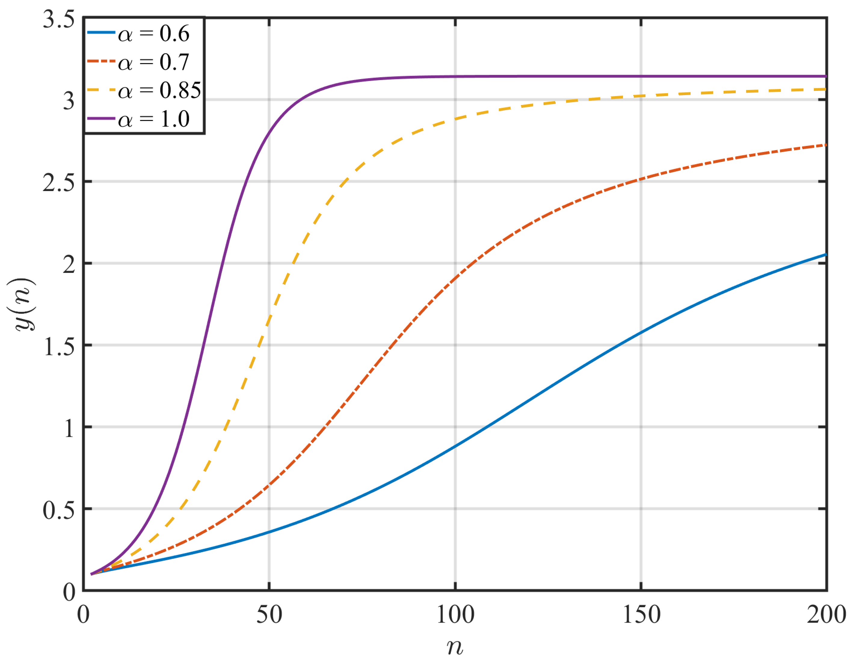
Using the iterative scheme derived from (28), we compute the numerical solution on ${[2,200]}_{\mathbb{Z}}$. First, we fix the initial value $y_0=0.1$ and vary the fractional order $\alpha \in \{0.6,0.7,0.85,1.0\}$ to examine the effect of the fractional order on the solution. The numerical results are displayed in Figure 1 and summarized in

Table 3. Numerical values of $y\left(n\right)$ for different fractional orders $\alpha$ with $y_0=0.1$.

n	$\mathit{\alpha }=0.6$	$\mathit{\alpha }=0.7$	$\mathit{\alpha }=0.85$	$\mathit{\alpha }=1.0$
5	0.117260	0.121061	0.126991	0.133026
10	0.139882	0.153509	0.179639	0.213805
20	0.184343	0.229437	0.341985	0.544411
30	0.233859	0.330486	0.627434	1.268744
40	0.291234	0.466286	1.083118	2.221098
50	0.358391	0.645216	1.654605	2.795671
60	0.436969	0.870663	2.156293	3.019729
70	0.528283	1.134517	2.488305	3.099047
80	0.633094	1.413794	2.686287	3.126756
90	0.751246	1.678530	2.805164	3.136419
100	0.881304	1.906856	2.879795	3.139789
120	1.164146	2.237763	2.963345	3.141373
140	1.446382	2.441840	3.006770	3.141566
160	1.695161	2.571926	3.032748	3.141589
180	1.896972	2.659914	3.049937	3.141592
200	2.054701	2.722810	3.062157	3.141593

. It is observed that for higher fractional orders, the solution grows rapidly in the early stage but eventually tends to a steady value; for lower orders, the solution grows more slowly and consistently stays below the higher-order solutions throughout the entire interval. This is consistent with the memory effect of fractional calculus: lower-order fractional differences possess stronger memory, resulting in smoother and slower evolution of the solution.

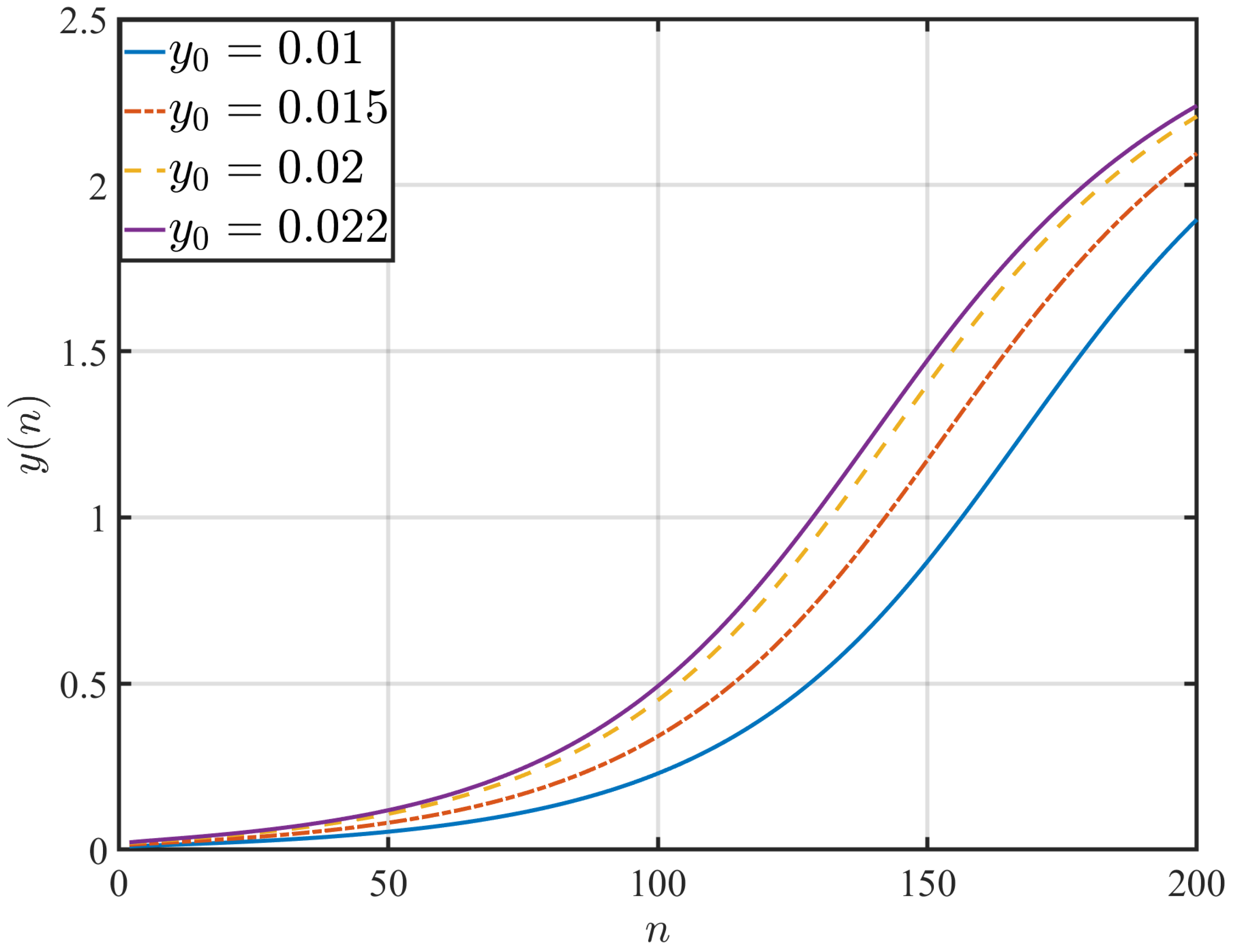
Second, we fix the fractional order $\alpha =2/3$ and vary the initial value $y_0\in \{0.01,0.015,0.02,0.022\}$ to investigate the sensitivity of the solution with respect to perturbations in the initial data. The numerical results are displayed in Figure 2 and summarized in

Table 4. Numerical values of $y\left(n\right)$ for different initial values $y_0$ with $\alpha =2/3$.

n	${\mathit{y}}_0=0.01$	${\mathit{y}}_0=0.015$	${\mathit{y}}_0=0.02$	${\mathit{y}}_0=0.022$
5	0.011982	0.017973	0.023963	0.026360
10	0.014881	0.022322	0.029762	0.032738
20	0.021309	0.031962	0.042614	0.046874
30	0.029450	0.044170	0.058884	0.064768
40	0.040072	0.060095	0.080103	0.088101
50	0.054068	0.081068	0.108027	0.118797
60	0.072581	0.108784	0.144885	0.159289
70	0.097103	0.145441	0.193526	0.212671
80	0.129591	0.193870	0.257541	0.282797
90	0.172582	0.257643	0.341273	0.374233
100	0.229320	0.341089	0.449579	0.491870
120	0.400749	0.586106	0.756191	0.819538
140	0.680089	0.953242	1.174453	1.249898
160	1.078253	1.396965	1.612418	1.678990
180	1.522246	1.800067	1.963325	2.011124
200	1.896430	2.095378	2.206667	2.238961

. It is clearly observed that the solution depends continuously on the initial value: small perturbations in $y_0$ lead to small, uniformly controlled deviations in the solution.

Verification of continuous dependence on initial data (Theorem 5).

To verify the Lipschitz continuous dependence of the solution on the initial data as established in Theorem 5, we fix the reference solution with $y_0=0.01$ and compute the maximum deviation ${max}_{n\in [2,200]}|y\left(n\right)-y_{\mathrm{ref}}\left(n\right)|$ for each perturbation $\delta = |y_0-0.01|$. The results are summarized in

Table 5. Sensitivity analysis: numerical deviations with theoretical Lipschitz bound.

Initial Perturbation $\mathit{\delta }$	Max Deviation	Ratio (Max Deviation/$\mathit{\delta }$)
0.005	0.318713	63.74
0.010	0.538308	53.83
0.012	0.609109	50.76

. For $\delta =0.005,0.010,0.012$, the ratios ${\displaystyle \frac{\mathrm{Max}\mathrm{deviation}}{\delta }}$ are $63.74$, $53.83$, and $50.76$, respectively. These values remain bounded as $\delta \to 0$, indicating that the solution depends Lipschitz continuously on the initial data, in agreement with Theorem 5. Moreover, by Lemma 8, the theoretical Lipschitz constant is explicitly given by $K={\left(1+{\displaystyle \frac{A}{\Gamma \left(\alpha \right)}}{\sum }_{k=1}^{N-a}{k}^{\overline{\alpha -1}}\right)}^{N-a}$, which is finite, thereby ensuring the existence of a uniform bound. This confirms that the numerical results are consistent with the theoretical prediction.

The ratio ${\displaystyle \frac{\mathrm{Max}\mathrm{deviation}}{\delta }}$ remains bounded (between 50 and 64) for all perturbations, indicating that the solution depends Lipschitz continuously on the initial data as predicted by Theorem 5.

Verification of the assumptions of Theorem 1.

Now consider the specific initial value problem

$$\left\{\begin{array}{c}{\Delta }^{{\displaystyle \frac{2}{3}}}y\left(n\right)={\displaystyle \frac{1}{10}}sin\left(n-{\displaystyle \frac{1}{3}}\right),n\in {[3,11]}_{\mathbb{Z}},\hfill \\ y\left(2\right)=0.1,\hfill \end{array}\right.$$

(29)

where $f[n,y\left(n\right)]={\displaystyle \frac{1}{10}}siny\left(n\right)$ for $n\in {[3,11]}_{\mathbb{Z}}$ and $y\left(n\right)\in \mathbb{R}$. The function f satisfies the Lipschitz condition with constant $L={\displaystyle \frac{1}{10}}$, since

$$|f(n,y_1)-f(n,y_2)| ={\displaystyle \frac{1}{10}}|sin{y}_1-sin{y}_2| \le {\displaystyle \frac{1}{10}}|y_1-y_2|.$$

Moreover, $|f(n,y)|\le {\displaystyle \frac{1}{10}}$, so the boundedness condition holds with $K={\displaystyle \frac{1}{10}}$. To verify the condition of Theorem 1, we note that for $a=2$, $\alpha ={\displaystyle \frac{2}{3}}$, and all $n\in [3,11]$, we have

$${\displaystyle \frac{{(\alpha +1)}^{\overline{n-a-1}}}{(n-a-1)!}}={\displaystyle \frac{{\left(\frac{5}{3}\right)}^{\overline{n-3}}}{(n-3)!}}\le 1,$$

and consequently $L={\displaystyle \frac{1}{10}}<1$ trivially satisfies the required inequality. Therefore, by Theorem 1, problem (29) possesses a unique solution on ${[3,11]}_{\mathbb{Z}}$.

Remark 2

(on numerical simulations for other examples). The other three types of fractional difference equations, namely the forward final value problem, backward initial value problem, and backward final value problem, can be treated similarly by using the iterative schemes derived from their corresponding Volterra-type summation equations (Theorems 2–4). Numerical validations for the four formulations have already been discussed in [23]. Since the main purpose of the present work is to establish the qualitative properties, including existence, uniqueness, and continuous dependence on initial/final data, Example 1 is presented as a representative numerical illustration of the continuous dependence result (Theorem 5). Similar simulations can be performed for the remaining cases to verify the corresponding theoretical results.

Example 2.

Consider the final value problem of the forward fractional difference equation

$$\left\{\begin{array}{c}{(-\Delta ) }^{{\displaystyle \frac{3}{4}}}y\left(n\right)={\displaystyle \frac{1}{20}}{\displaystyle \frac{y\left(n\right)}{1+|y(n)|}},n\in {[1,14]}_{\mathbb{Z}},\hfill \\ y\left(15\right)=0.1,\hfill \end{array}\right.$$

(30)

where $f[n,y\left(n\right)]={\displaystyle \frac{1}{20}}{\displaystyle \frac{y\left(n\right)}{1+|y(n)|}}$ for $n\in {[1,14]}_{\mathbb{Z}}$ and $y\left(n\right)\in \mathbb{R}$. The function f satisfies the Lipschitz condition with constant $L={\displaystyle \frac{1}{20}}$, because the mapping $g\left(y\right)=y/(1+|y|)$ is Lipschitz with constant 1 (its derivative is bounded by 1). Indeed,

$$|f(n,y_1)-f(n,y_2)| \le {\displaystyle \frac{1}{20}}|y_1-y_2|.$$

Clearly, $|f(n,y)|\le {\displaystyle \frac{1}{20}}$, so the boundedness condition holds with $M={\displaystyle \frac{1}{20}}$. For Theorem 2, with $b=15$, $\alpha ={\displaystyle \frac{3}{4}}$, and any $n\in [1,14]$, we have

$${\displaystyle \frac{{(\alpha +1)}^{\overline{b-n-1}}}{(b-n-1)!}}={\displaystyle \frac{{\left(\frac{7}{4}\right)}^{\overline{14-n}}}{(14-n)!}}\le 1,$$

which implies that the contraction condition $L<1$ is automatically satisfied. Thus, by Theorem 2, problem (30) admits a unique solution on ${[1,14]}_{\mathbb{Z}}$.

Example 3.

Consider the initial value problem of the backward fractional difference equation

$$\left\{\begin{array}{c}{\mathsf{\nabla }}^{{\displaystyle \frac{1}{2}}}y\left(n\right)={\displaystyle \frac{1}{5}}arctany\left(n\right),n\in {[2,10]}_{\mathbb{Z}},\hfill \\ y\left(1\right)=0.1,\hfill \end{array}\right.$$

(31)

where $f[n,y\left(n\right)]={\displaystyle \frac{1}{5}}arctany\left(n\right)$ for $n\in {[2,10]}_{\mathbb{Z}}$ and $y\left(n\right)\in \mathbb{R}$. The function f satisfies the Lipschitz condition with constant $L={\displaystyle \frac{1}{5}}$, because $|arctan{y}_1-arctan{y}_2| \le |y_1-y_2|$ (the derivative of arctan is bounded by 1). Thus,

$$|f(n,y_1)-f(n,y_2)| \le {\displaystyle \frac{1}{5}}|y_1-y_2|.$$

Moreover, $|f(n,y)|\le {\displaystyle \frac{\pi }{10}}\le {\displaystyle \frac{1}{2}}$, so the boundedness condition holds with $M={\displaystyle \frac{1}{2}}$. For Theorem 3, with $a=1$, $\alpha ={\displaystyle \frac{1}{2}}$, and any $n\in [2,10]$, we have

$${\displaystyle \frac{{(\alpha +1)}^{\overline{n-a-1}}}{(n-a-1)!}}={\displaystyle \frac{{\left(\frac{3}{2}\right)}^{\overline{n-2}}}{(n-2)!}}\le 1,$$

hence $L={\displaystyle \frac{1}{5}}<1$ guarantees the contraction property. Consequently, by Theorem 3, problem (31) has a unique solution on ${[2,10]}_{\mathbb{Z}}$.

Example 4.

Consider the final value problem of the backward fractional difference equation

$$\left\{\begin{array}{c}{(-\mathsf{\nabla }) }^{{\displaystyle \frac{4}{5}}}y\left(n\right)={\displaystyle \frac{1}{15}}{\displaystyle \frac{y\left(n-\frac{1}{5}\right)}{1+\left|y\left(n-\frac{1}{5}\right)\right|}},n\in {[1,9]}_{\mathbb{Z}},\hfill \\ y\left(10\right)=0.1,\hfill \end{array}\right.$$

(32)

where $f[n,y\left(n\right)]={\displaystyle \frac{1}{15}}{\displaystyle \frac{y\left(n\right)}{1+|y(n)|}}$ for $n\in {[1,9]}_{\mathbb{Z}}$ and $y\left(n\right)\in \mathbb{R}$. As argued in Example 2, the function $g\left(y\right)=y/(1+|y|)$ is Lipschitz with constant 1, so

$$|f(n,y_1)-f(n,y_2)| \le {\displaystyle \frac{1}{15}}|y_1-y_2|,$$

i.e., the Lipschitz constant is $L={\displaystyle \frac{1}{15}}$. Clearly $|f(n,y)|\le {\displaystyle \frac{1}{15}}$, so boundedness holds with $M={\displaystyle \frac{1}{15}}$. For Theorem 4, with $b=10$, $\alpha ={\displaystyle \frac{4}{5}}$, and any $n\in [1,9]$, we have

$${\displaystyle \frac{{(\alpha +1)}^{\overline{b-n-1}}}{(b-n-1)!}}={\displaystyle \frac{{\left(\frac{9}{5}\right)}^{\overline{9-n}}}{(9-n)!}}\le 1,$$

which together with $L<1$ satisfies the conditions of Theorem 4. Hence, problem (32) possesses a unique solution on ${[1,9]}_{\mathbb{Z}}$.

These four examples cover all four types of Liouville–Caputo fractional difference equations discussed in Section 3 and demonstrate the applicability of the corresponding existence and uniqueness theorems. In each case, the chosen nonlinearities satisfy the required Lipschitz and boundedness conditions, and the inequalities involving the fractional factorials are automatically fulfilled due to the elementary estimate ${\displaystyle \frac{{(\alpha +1)}^{\overline{k}}}{k!}}\le 1$ for all $k\ge 0$ and $\alpha \in (0,1]$.

Example 5

(Economics: fractional inventory adjustment with memory). Consider the initial value problem of the forward fractional difference equation

$$\left\{\begin{array}{c}{\Delta }^{{\displaystyle \frac{1}{2}}}Q\left(n\right)=0.2·{\displaystyle \frac{Q\left(n+\frac{1}{2}\right)}{1+\left|Q\left(n+\frac{1}{2}\right)\right|}}·\left(1-e^{-\left|Q(n+{\displaystyle \frac{1}{2}})\right|}\right),n\in {[0,3]}_{\mathbb{Z}},\hfill \\ Q\left(0\right)=10,\hfill \end{array}\right.$$

(33)

where $Q\left(n\right)$ denotes the inventory level (in thousand units) at week n. Define $f(n,Q)=0.2{\displaystyle \frac{Q}{1+|Q|}}(1-e^{-|Q|})$. It is clear that $|f(n,Q)|\le 0.2$ for all Q, so condition (H1) holds with $M=0.2$. Moreover, the function f is Lipschitz with constant $A=0.4$ because the derivative of ${\displaystyle \frac{Q}{1+|Q|}}(1-e^{-|Q|})$ is bounded by 2. Hence, $|f(n,Q_1)-f(n,Q_2)| \le 0.4|Q_1-Q_2|$. For Theorem 1 (with $a=0$, $\alpha ={\displaystyle \frac{1}{2}}$), one verifies that for every $n=1,2,3,4$ the inequality $0.4<{\displaystyle \frac{(n-1)!}{{\left(1.5\right)}^{\overline{n-1}}}}$ holds (the smallest right-hand side is about $0.667$ at $n=2$, still larger than $0.4$), and $A=0.4<1$. Thus, all assumptions of Theorem 1 are satisfied, guaranteeing a unique solution $Q\left(n\right)$ for $n=0,1,2,3,4$.

Example 6

(Economics: inflation deviation with terminal condition). Consider the final value problem of the forward fractional difference equation of order $\alpha =0.8$, describing the evolution of inflation deviation $\pi \left(n\right)$ (in percentage points) over $n=0,1,2,3,4$ with terminal condition at $b=5$:

$$\left\{\begin{array}{c}{(-\Delta ) }^{0.8}\pi \left(n\right)=0.1·{\displaystyle \frac{\pi \left(n\right)}{1+|\pi (n)|}}·\left(1-e^{-|\pi (n)|}\right),n\in {[0,4]}_{\mathbb{Z}},\hfill \\ \pi \left(5\right)=1.5,\hfill \end{array}\right.$$

(34)

where $\pi \left(n\right)$ denotes the deviation of inflation from a target value (e.g., 2%). The nonlinear function $f(n,\pi )=0.1{\displaystyle \frac{\pi }{1+|\pi |}}(1-e^{-|\pi |})$ models a central bank’s bounded adjustment rule. Clearly $|f(n,\pi )|\le 0.1$ (condition (H1)), and f is Lipschitz with constant $A=0.2$ because the derivative of ${\displaystyle \frac{\pi }{1+|\pi |}}(1-e^{-|\pi |})$ is bounded by 2. Hence, $|f(n,{\pi }_1)-f(n,{\pi }_2)| \le 0.2|{\pi }_1-{\pi }_2|$.

For Theorem 2, we set $b=5$, $\alpha =0.8$ ($\alpha +1=1.8$). For each $n=0,1,2,3,4$, one easily checks that $0.2<{\displaystyle \frac{(b-1-n)!}{{\left(1.8\right)}^{\overline{b-1-n}}}}$ holds (the smallest right-hand side is about $0.261$ at $n=0$, still larger than $0.2$). Also, $A=0.2<1$. Therefore, all conditions of Theorem 2 are satisfied, and the problem possesses a unique solution $\pi \left(n\right)$ for $n=0,\dots ,5$. This means that given a known future inflation deviation $\pi \left(5\right)=1.5\%$ (e.g., a policy target), the past path $\pi \left(n\right)$ is uniquely determined. Such backward analysis is valuable for policy evaluation and calibration.

5. Conclusions

In this paper, we have established a unified well-posedness framework for four Liouville–Caputo fractional difference formulations on finite discrete intervals, including forward and backward difference operators with variable upper- and lower-limit fractional sums. By using the equivalence between the considered problems and their associated Volterra-type summation equations, sufficient conditions for the existence and uniqueness of solutions have been obtained via the Banach contraction mapping principle. Moreover, the Lipschitz continuous dependence of solutions on prescribed initial or final data has been proved through explicit estimates derived from a discrete fractional Gronwall-type inequality. The numerical experiments further illustrate the theoretical results, particularly the sensitivity of solutions with respect to the fractional order and boundary data. These results complement the unified operator framework developed in [23] by providing essential qualitative properties of the corresponding solutions. Future work will focus on relaxing the assumptions on the nonlinear term, extending the analysis to higher-order fractional differences with multiple initial or final conditions, and investigating stability and numerical approximation theories for broader classes of discrete fractional systems.

References

1. Caputo, M. Linear models of dissipation whose Q is almost frequency independent—II. Geophys. J. R. Astron. Soc. 1967, 13, 529–539. [Google Scholar] [CrossRef] [Scilit]
2. Yang, B.; Wang, Z.; Tian, H.; Liu, J. Symplectic Dynamics and Simultaneous Resonance Analysis of Memristor Circuit Based on Its Van der Pol Oscillator. Symmetry 2022, 14, 1251. [Google Scholar] [CrossRef] [Scilit]
3. Berkal, M.; Almatrafi, M.B.; Semmar, B.; Navarro, J.F. Dynamical analysis of a generalized conformable incommensurate fractional-order modified SIR epidemic model. J. Appl. Math. Comput. 2026, 72, 30. [Google Scholar]
4. Zhang, R.; Xi, X.; Tian, H.; Wang, Z. Dynamical analysis and finite-time synchronization for a chaotic system with hidden attractor and surface equilibrium. Axioms 2022, 11, 579. [Google Scholar] [CrossRef] [Scilit]
5. Yang, R.; Tian, H.; Wang, Z.; Wang, W.; Zhang, Y. Dynamical Analysis and Synchronization of Complex Network Dynamic Systems under Continuous-Time. Symmetry 2024, 16, 687. [Google Scholar] [CrossRef] [Scilit]
6. Cheow, Y.H.; Ng, K.H.; Phang, C.; Ng, K.H. The application of fractional calculus in economic growth modelling. Heliyon 2024, 10, e35379. [Google Scholar] [CrossRef] [Scilit] [PubMed]
7. Shaikhet, L. Lyapunov Functionals and Stability of Stochastic Functional Differential Equations; Springer: Berlin/Heidelberg, Germany, 2013. [Google Scholar]
8. Wang, Z.; Tian, H.; Krejcar, O.; Namazi, H. Synchronization in a network of map-based neurons with memristive synapse. Eur. Phys. J. Spec. Top. 2022, 231, 4057–4064. [Google Scholar] [CrossRef] [Scilit]
9. Kocic, V.L.; Ladas, G. Global Behavior of Nonlinear Difference Equations of Higher Order with Applications; Springer: Berlin/Heidelberg, Germany, 1993. [Google Scholar]
10. Agarwal, R.P. Difference Equations and Inequalities: Theory, Methods, and Applications; CRC Press: Boca Raton, FL, USA, 2000. [Google Scholar]
11. Oldham, K.; Spanier, J. The Fractional Calculus: Theory and Applications of Differentiation and Integration to Arbitrary Order; Elsevier: Amsterdam, The Netherlands, 1974. [Google Scholar]
12. Kilbas, A.A.; Srivastava, H.M.; Trujillo, J.J. Theory and Applications of Fractional Differential Equations; Elsevier: Amsterdam, The Netherlands, 2006. [Google Scholar]
13. Podlubny, I. Fractional Differential Equations; Academic Press: Cambridge, MA, USA, 1999. [Google Scholar]
14. Yao, Z.; Yang, Z.; Gao, J. Unconditional stability analysis of Grunwald Letnikov method for fractional-order delay differential equations. Chaos Solitons Fractals 2023, 177, 114193. [Google Scholar] [CrossRef] [Scilit]
15. Wu, G.C.; Baleanu, D.; Xie, H.P. Riesz Riemann-Liouville difference on discrete domains. Chaos Interdiscip. J. Nonlinear Sci. 2016, 26, 084308. [Google Scholar] [CrossRef] [Scilit]
16. Abdeljawad, T. On Riemann and Caputo fractional differences. Comput. Math. Appl. 2011, 62, 1602–1611. [Google Scholar] [CrossRef] [Scilit]
17. Goodrich, C.; Peterson, A.C. Discrete Fractional Calculus; Springer: Berlin/Heidelberg, Germany, 2015. [Google Scholar]
18. Laledj, N.; Salim, A.; Lazreg, J.E.; Abbas, S.; Ahmad, B.; Benchohra, M. On implicit fractional q-difference equations: Analysis and stability. Math. Methods Appl. Sci. 2022, 45, 10775–10797. [Google Scholar] [CrossRef] [Scilit]
19. Allouch, N.; Graef, J.R.; Hamani, S. Boundary Value Problem for Fractional q-Difference Equations with Integral Conditions in Banach Spaces. Fractal Fract. 2022, 6, 237. [Google Scholar] [CrossRef] [Scilit]
20. Alili, F.; Amara, A.; Zennir, K.; Radwan, T. On Hybrid and Non-Hybrid Discrete Fractional Difference Inclusion Problems for the Elastic Beam Equation. Fractal Fract. 2024, 8, 486. [Google Scholar] [CrossRef] [Scilit]
21. Hattaf, K. On the Stability and Numerical Scheme of Fractional Differential Equations with Application to Biology. Computation 2022, 10, 97. [Google Scholar] [CrossRef] [Scilit]
22. Cheng, J.F.; Chu, Y.M. Fractional Difference Equations with Real Variable. Abstr. Appl. Anal. 2012, 2012, 918529. [Google Scholar] [CrossRef] [Scilit]
23. Li, X.; Tian, H.; Zhang, P.; Ma, J. Unified framework of four Caputo fractional differences for initial and final value problems in discrete fractional calculus with variable bounds. Adv. Differ. Equ. Control Process. 2026, 33, 3725. [Google Scholar]
24. Salem, A.; Mshary, N. On the Existence and Uniqueness of Solution to Fractional-Order Langevin Equation. Adv. Math. Phys. 2020, 2020, 8890575. [Google Scholar] [CrossRef] [Scilit]
25. Nanware, J.A.; Dhaigude, D.B. Existence and uniqueness of solutions of differential equations of fractional order with integral boundary conditions. J. Nonlinear Sci. Appl. 2014, 7, 246–254. [Google Scholar] [CrossRef] [Scilit]
26. Ahmad, B.; Alsaedi, A. Existence and uniqueness of solutions for coupled systems of higher-order nonlinear fractional differential equations. Fixed Point Theory Appl. 2010, 2010, 364560. [Google Scholar] [CrossRef] [Scilit]
27. Ardjouni, A.; Djoudi, A. Existence and uniqueness of positive solutions for first-order nonlinear Liouville–Caputo fractional differential equations. São Paulo J. Math. Sci. 2020, 14, 381–390. [Google Scholar]
28. Baroudi, S.; Kassidi, A.; El Mfadel, A.; Elomari, M. Coincidence degree theory for higher order nonlinear fractional differential equations: Existence and uniqueness results. Commun. Nonlinear Sci. Numer. Simul. 2025, 147, 108847. [Google Scholar] [CrossRef] [Scilit]
29. Benzenati, D.; Bouriah, S.; Salim, A.; Benchohra, M. Existence and uniqueness of periodic solutions for some nonlinear ψ-fractional coupled systems. Vietnam J. Math. 2025, 53, 389–406. [Google Scholar]
30. Azzouz, B.; Beddani, M. Existence and uniqueness of solutions for a class from fractional differential equations involving a left χ-Hilfer derivative. Math. Methods Appl. Sci. 2025, 48, 15132–15139. [Google Scholar] [CrossRef] [Scilit]
31. Promsakon, C.; Ansari, I.; Wetsah, M.; Kumar, A.; Karthikeyan, K.; Sitthiwiratttham, T. Existence and uniqueness of solutions for fractional-differential equation with boundary condition using nonlinear multi-fractional derivatives. Math. Probl. Eng. 2024, 2024, 6844686. [Google Scholar] [CrossRef] [Scilit]
32. Graef, J.R.; Kong, L.; Wang, M. Existence and uniqueness of solutions for a fractional boundary value problem on a graph. Fract. Calc. Appl. Anal. 2014, 17, 499–510. [Google Scholar] [CrossRef] [Scilit]
33. Ezugorie, I.G.; Ahman, Q.O.; Agbata, B.C.; Atabo, V.O.; Senewo, E.O.; Micheal, B.D. Analysis of existence and uniqueness of solutions of fractional-order mathematical model of HIV/AIDS. J. Basics Appl. Sci. Res. 2025, 3, 40–51. [Google Scholar] [CrossRef] [Scilit]
34. Islam, M.N.; Koyuncuoglu, H.C.; Raffoul, Y.N. A note on the existence of solutions for Caputo fractional differential equations. J. Integral Equ. Appl. 2024, 36, 437–446. [Google Scholar] [CrossRef] [Scilit]
Figure 1. Numerical solutions y ( n ) for different fractional orders α in Example 1 with y 0 = 0.1 .
Fractalfract 10 00504 g001
Figure 2. Numerical solutions y ( n ) for different initial values y 0 in Example 1 with α = 2 / 3 .
Fractalfract 10 00504 g002