Implicit Fractional Differential Equation with Time-Varying State-Dependent Feedback

Abstract

The present article introduces and investigates a class of implicit fractional differential equations with time-varying state-dependent feedback, a setting that significantly extends existing fractional delay models. Existence and uniqueness results are established via the Banach fixed-point theorem, while sharp exponential growth estimates for the solutions are derived using a generalized Gronwall-type inequality. These results provide new analytical insights into the qualitative behavior of fractional systems with dynamically evolving feedback mechanisms.

1. Introduction

Delay differential equations play a fundamental role in modeling and predicting processes in the life sciences, including population dynamics, immunology, and neural networks. Fractional delay systems exhibit rich dynamical behavior arising from the combined effects of memory and temporal shifts, leading to nonlocal temporal dynamics. Such models naturally describe immune responses and viral dynamics, as fractional memory captures biological history dependence. In addition, fractional delay formulations are effective in modeling viscoelastic aftereffects, distributed transport, processing delays, and may induce complex phenomena such as Hopf bifurcation at non-integer delays; see [1,2,3] and their references. A delay differential system with fixed delay is independent of the past state of the system. In contrast, past dependence on a variable is captured through state-dependent delays. Unlike constant or time-dependent delays, state-dependent delays evolve dynamically with the solution itself, rendering the system highly nonlinear and more realistic for modeling complex processes involving memory and feedback mechanisms. Such equations naturally arise in situations where the reaction time of a system depends on its current state, including population dynamics with density-dependent maturation periods, physiological and neural models with adaptive response delays, control systems with feedback-dependent latency, and economic systems in which decision delays are influenced by prevailing market conditions. Recently, there has been growing interest in the study of state-dependent delays due to their strong modeling capabilities and wide range of applications. For instance, Darwish [4] investigated the existence of solutions for initial value problems associated with fractional functional differential equations and neutral functional differential equations with state-dependent delay. Benchohra et al. [5] established the existence of mild solutions for semilinear fractional integro-differential inclusions involving state-dependent delay. Furthermore, Belmekki et al. [6] examined the existence of mild solutions for semilinear functional differential equations of fractional order with state-dependent delay. For more related studies we refer the reader to [7,8,9,10,11] and references within.

In 2025, Baleg et al. [12] employed fixed-point theorems and theoretical analytical techniques to investigate a class of fractional delay differential equations. As an application, Arthur et al. [13] studied the controllability of a stochastic fractional system with state-dependent feedback and impulsive effect. Liang et al. [14] proved the existence of unique regular solutions for a fractional integro-differential equation with state-dependent feedback. For similar results, see [15,16] and the references therein, which highlight both theoretical developments and applications of state-dependent delay systems.

The present paper investigates an implicit time-varying delay variable for an implicit fractional differential equation. Precisely, we consider

$$\begin{array}{c}\hfill \left\{\begin{array}{c}{}^C\mathcal{D}_t^{\alpha }x(t)={\lambda }_{1}f(t,x(t),{}^C\mathcal{D}_t^{\alpha }x(t))+{\lambda }_{2}g(t,x(t-\tau (t,x(t))),{}^C\mathcal{D}_t^{\alpha }x(t)),t\in (0,T],\hfill \\ \\ x(t)=h(t),t\in [-{\tau }^{*},0],{\tau }^{*}>0,\hfill \end{array}\right.\end{array}$$

(1)

where ${}^C\mathcal{D}_t^{\alpha },\alpha \in (0,1)$ is a Caputo fractional differential operator, $f,g:[0,T]\times {\mathbb{R}}^2\to \mathbb{R}$ are Lipschitz continuous functions, and $h\in C([-{\tau }^{*},0],\mathbb{R})$ and ${\lambda }_1,{\lambda }_2$ are positive parameters. The state-dependent delay function $\tau \in C([0,T]\times \mathbb{R},\mathbb{R})$ is assumed to be positive and bounded, and the maximum delay ${\tau }^{*}$ such that

$$\tau (t,x(t))\le {\tau }^{*}.$$

Define $C^{*}=C([-{\tau }^{*},T],\mathbb{R})$ — a Banach space of continuous functions equipped with a norm

$$\parallel x\parallel =\underset{t\in [-{\tau }^{*},T]}{sup}|x(t)|.$$

Alternatively, for each t, one defines the maximum delay ${\tau }^{*}$ by

$${\tau }^{*}=\underset{x\in C^{*}}{sup}\tau (t,x).$$

(2)

Remark 1.

Here, we give some insights into the formulation:

1.

Note that the supremum in Equation (2) is taken over a range of real valued functions for each t.

2.

The model studied in Equation (1) assumes that the delay function depends on the current state $x(t)$ rather than the delayed state $x(t-\tau )$. This formulation is particularly appropriate in situations where the present state determines the duration of a future process or where the current state directly governs future delays through environmental, physiological, or operational effects. Such state-dependent delays arise naturally in a variety of applications. For example, in population dynamics, the current population density may influence the maturation period of newborns, as overcrowding or limited resources can retard development. In epidemiology, the current immune status or pathogen load may affect the incubation period of an infectious disease. In manufacturing systems, the current workload determines processing or waiting times, while in traffic flow models, the prevailing traffic density influences drivers’ reaction times and travel delays. Consequently, modeling the delay as a function of the current state provides a realistic representation of systems in which present conditions regulate future temporal responses.

3.

The model in Equation (1) encompasses both delayed and non-delayed implicit fractional differential equations. Specifically, it reduces to a non-delayed implicit fractional differential equation when ${\lambda }_2=0$, and to a delayed implicit fractional differential equation when ${\lambda }_1=0$.

4.

The implicit formulation naturally captures situations in which the evolution of the system depends simultaneously on both the current and delayed states through nonlinear relationships. This framework provides greater modeling flexibility by accommodating complex interactions, state-dependent constraints, memory effects, and nonlinear feedback mechanisms that may not be adequately represented by explicit formulations. Consequently, implicit partial differential equations offer a more general and realistic mathematical model for describing phenomena in continuum mechanics, porous media flow, biological systems, epidemiology, and stochastic fractional dynamics, where the underlying governing equations often arise in an implicit form.

The structure of the paper is organized as follows: Section 2 introduces the preliminary concepts required for the subsequent analysis. Section 3 presents the auxiliary results that serve as essential tools for establishing the main findings. Section 4 contains the principal results of the paper, including formal statements and detailed proofs. Finally, Section 5 provides a summary of the results and concluding remarks.

2. Preliminary Concepts

Definition 1.

The Riemann–Liouville (R-L) fractional integral of order $\alpha >0$ for $u\in C([0,\infty ),\mathbb{R})$ is defined by

$${\mathcal{I}}_t^{\alpha }u(t)={\displaystyle \frac{1}{\mathrm{\Gamma }(\alpha )}}{\int }_0^t{(t-s)}^{\alpha -1}u(s)ds,t>0.$$

Definition 2.

The Caputo fractional derivative of order $\alpha \in (0,1)$ for $u\in C([0,\infty ),\mathbb{R})$ is defined by

$${}^C\mathcal{D}_t^{\alpha }u(t)={\displaystyle \frac{1}{\mathrm{\Gamma }(1-\alpha )}}{\int }_0^t{(t-s)}^{-\alpha }{u}^{\prime }(s)ds,t>0.$$

Lemma 1

(Lemma 2.2 in [17], Generalized Gronwall Inequality). Suppose $\alpha >0,\theta (t)$ is a nonnegative function locally integrable on $[0,T],T\le \infty$, and $\hslash (t)$ is a nonnegative, nondecreasing continuous function defined on $[0,T]$, $\hslash (t)\le M$, and suppose $\psi (t)$ is nonnegative and locally integrable on $[0,T]$ with

$$\psi (t)\le \theta (t)+\hslash (t){\int }_0^t{(t-s)}^{\alpha -1}\psi (s)ds,$$

then

$$\psi (t)\le \theta (t)+\hslash (t){\int }_0^t{\displaystyle \sum _{k=1}^{\infty }}\left[{\displaystyle \frac{{(\hslash (t)\mathrm{\Gamma }(\alpha ))}^k}{\mathrm{\Gamma }(k\alpha )}}{(t-s)}^{k\alpha -1}\theta (s)\right]ds,t\in [0,T].$$

Corollary 1.

Under the hypothesis of Lemma 1, let θ be a nondecreasing function on $[0,T]$, then

$$\psi (t)\le \theta (t)E_{\alpha }[\hslash (t)\mathrm{\Gamma }(\alpha )t^{\alpha }],t\in [0,T].$$

3. Auxiliary Results

Here, we present some results that will be needed to prove our major results. The following conditions are imposed to ensure the well-posedness of the problem:

Condition 1.

The nonlinear functions $f,g:[0,T]\times {\mathbb{R}}^2\to \mathbb{R}$ are said to satisfy the following Lipschitz condition

$$|f(t,x_1,x_2)-f(t,y_1,y_2)|\le {\ell }_f(|x_1-y_1|+|x_2-y_2|),\forall t\in [0,T],$$

and consequently,

$$|f(t,x_1,x_2)|\le |f(t,0,0)|+{\ell }_f(|x_1|+|x_2|)\le c_0+{\ell }_f(|x_1|+|x_2|),$$

where $c_0$ is some positive constant. The function g also satisfies the same conditions.

Lemma 2

(Continuity of the differential operator). For $0<{\lambda }_1{\ell }_f+{\lambda }_2{\ell }_g<1$, the fractional derivative operator satisfies the following:

$$\begin{array}{cc}\hfill |{}^C\mathcal{D}_t^{\alpha }x(t)-{}^C\mathcal{D}_t^{\alpha }y(t)|\le & {\displaystyle \frac{{\lambda }_1{\ell }_f}{1-({\lambda }_1{\ell }_f+{\lambda }_2{\ell }_g)}}|x(t)-y(t)|\hfill \\ & +{\displaystyle \frac{{\lambda }_2{\ell }_g}{1-({\lambda }_1{\ell }_f+{\lambda }_2{\ell }_g)}}|x(t-\tau (t,x(t)))-y(t-\tau (t,y(t)))|.\hfill \end{array}$$

Furthermore,

$$\begin{array}{cc}\hfill |{}^C\mathcal{D}_t^{\alpha }x(t)|\le {\displaystyle \frac{({\lambda }_1+{\lambda }_2)c_0}{1-({\lambda }_1{\ell }_f+{\lambda }_2{\ell }_g)}}& +{\displaystyle \frac{{\lambda }_1{\ell }_f}{1-({\lambda }_1{\ell }_f+{\lambda }_2{\ell }_g)}}|x(t)|\hfill \\ & +{\displaystyle \frac{{\lambda }_2{\ell }_g}{1-({\lambda }_1{\ell }_f+{\lambda }_2{\ell }_g)}}|x(t-\tau (t,x(t)))|.\hfill \end{array}$$

Proof. 

The proof is obtained by applying Condition 1. We proceed as follows:

$$\begin{array}{cc}\hfill |{}^C\mathcal{D}_t^{\alpha }x(t)-{}^C\mathcal{D}_t^{\alpha }y(t)|\le & {\lambda }_1|f(t,x(t),{}^C\mathcal{D}_t^{\alpha }x(t))-f(t,y(t),{}^C\mathcal{D}_t^{\alpha }y(t))|\hfill \\ \hfill +& {\lambda }_2|g(t,x(t-\tau (t,x(t))),{}^C\mathcal{D}_t^{\alpha }x(t))-g(t,y(t-\tau (t,y(t))),{}^C\mathcal{D}_t^{\alpha }y(t))|\hfill \\ \hfill \le & {\lambda }_1{\ell }_f\left[|x(t)-y(t)|+|{}^C\mathcal{D}_t^{\alpha }x(t)-{}^C\mathcal{D}_t^{\alpha }y(t)|\right]\hfill \\ \hfill +& {\lambda }_2{\ell }_g\left[|x(t-\tau (t,x(t)))-y(t-\tau (t,x(t)))|+|{}^C\mathcal{D}_t^{\alpha }x(t)-{}^C\mathcal{D}_t^{\alpha }y(t)|\right].\hfill \end{array}$$

Collecting like terms, one arrives at

$$\begin{array}{cc}\hfill |{}^C\mathcal{D}_t^{\alpha }x(t)-{}^C\mathcal{D}_t^{\alpha }y(t)|\left[1-({\lambda }_1{\ell }_f+{\lambda }_2{\ell }_g)\right]\le & {\lambda }_1{\ell }_f|x(t)-y(t)|\hfill \\ & +{\lambda }_2{\ell }_g|x(t-\tau (t,x(t)))-y(t-\tau (t,x(t)))|,\hfill \end{array}$$

and the first part follows. To prove the second part, let $y(t)=0$ to obtain

$$\begin{array}{cc}\hfill |{}^C\mathcal{D}_t^{\alpha }x(t)|\le & {\lambda }_1|f(t,x(t),{}^C\mathcal{D}_t^{\alpha }x(t))-f(t,0,0)|+{\lambda }_2|g(t,x(t-\tau (t,x(t))),{}^C\mathcal{D}_t^{\alpha }x(t))-g(t,0,0)|\hfill \\ \hfill \le & {\lambda }_1|f(t,x(t),{}^C\mathcal{D}_t^{\alpha }x(t))|+{\lambda }_1|f(t,0,0)|+{\lambda }_2|g(t,x(t-\tau (t,x(t))),{}^C\mathcal{D}_t^{\alpha }x(t))|\hfill \\ & +{\lambda }_2|g(t,0,0)|\hfill \\ \hfill \le & {\lambda }_1{\ell }_f|x(t)|+{\lambda }_1{\ell }_f|{}^C\mathcal{D}_t^{\alpha }x(t))|+2{\lambda }_1|f(t,0,0)|+{\lambda }_2{\ell }_g|x(t-\tau (t,x(t)))|\hfill \\ & +{\lambda }_2{\ell }_g|{}^C\mathcal{D}_t^{\alpha }x(t))|+2{\lambda }_2|g(t,0,0)|\hfill \\ \hfill \le & {\lambda }_1|f(t,x(t),{}^C\mathcal{D}_t^{\alpha }x(t))|+{\lambda }_1|f(t,0,0)|+{\lambda }_2|g(t,x(t-\tau (t,x(t))),{}^C\mathcal{D}_t^{\alpha }x(t))|\hfill \\ & +{\lambda }_2|g(t,0,0)|\hfill \\ \hfill \le & {\lambda }_1{\ell }_f|x(t)|+{\lambda }_1{\ell }_f|{}^C\mathcal{D}_t^{\alpha }x(t))|+{\lambda }_1{c}_0+{\lambda }_2{\ell }_g|x(t-\tau (t,x(t)))|+{\lambda }_2{\ell }_g|{}^C\mathcal{D}_t^{\alpha }x(t))|\hfill \\ & +{\lambda }_2{c}_0.\hfill \end{array}$$

Now, collect like terms to arrive at

$$\begin{array}{c}\hfill |{}^C\mathcal{D}_t^{\alpha }x(t)|[1-({\lambda }_1{\ell }_f+{\lambda }_2{\ell }_g)]\le ({\lambda }_1+{\lambda }_2)c_0+{\lambda }_1{\ell }_f|x(t)|+{\lambda }_2{\ell }_g|x(t-\tau (t,x(t)))|,\end{array}$$

and the proof follows immediately.  □

We make further assumptions as follows

(H₁)

Assume $t-\tau (t,x(t))\le 0,\forall t\in [0,{\tau }^{*}].$

This implies that the delay term preserves the system state in the initial history region or interval.

(H₂)

Define the following set:

$$\begin{array}{c}\hfill D=\left\{\begin{array}{c}x\in C^{*}:|x(t-\tau (t,x(t)))|\le h(t)|x(t)|\mathrm{with}\parallel h\parallel \le {\gamma }_1,\forall t\in [0,{\tau }^{*}],\hfill \\ \\ x\in C^{*}:|x(t-\tau (t,x(t)))|\le q(t)|x(t)|\mathrm{with}\parallel q\parallel \le {\gamma }_2,\forall t\in [{\tau }^{*},T].\hfill \end{array}\right.\end{array}$$

Remark 2.

The idea of the assumption is as follows:

1.

In $(H_1)$: since $\tau (t,x(t))\le {\tau }^{*}$, then for $t\in [0,{\tau }^{*}]$, one gets $-{\tau }^{*}\le t-{\tau }^{*}\le t-\tau (t,x(t))\le 0,$ and thus, $t-\tau (t,x(t))\in [-{\tau }^{*},0].$

2.

For $(H_2)(a),$ let $t\in [0,{\tau }^{*}]$, and since $t-\tau (t,x(t))\in [-{\tau }^{*},0],$ then $x(t-\tau (t,x(t)))=h(t-\tau (t,x(t)))$ with h a history function. Hence, the assumption that $|x(t-\tau (t,x(t)))|\le h(t)|x(t)|.$

3.

Similarly, for $(H_2)(b)$, let $t\in [{\tau }^{*},T]$ which implies that $t-{\tau }^{*}\in [0,T-{\tau }^{*}]\subset [0,T]$. Since $\tau (t,x(t))\le {\tau }^{*}$ it follows that $0\le t-{\tau }^{*}\le t-\tau (t,x(t))\le t\le T$, thus, we assume that $|x(t-\tau (t,x(t)))|\le q(t)|x(t)|$ for some continuous function q.

4.

As a direction for future research, we intend to characterize the set D in terms of the delay function τ and construct explicit example of such a delay function.

Next, we formulate and make sense of the solution to Equation (1).

Theorem 1.

Let Condition 1 and Lemma 2 hold. Then, $x\in C^{*}$ is a solution to Equation (1) if and only if x satisfies

$$\begin{array}{c}\hfill \left\{\begin{array}{c}{\displaystyle x(t)=h(0)+\frac{{\lambda }_1}{\mathrm{\Gamma }(\alpha )}{\int }_0^t{(t-s)}^{\alpha -1}f(s,x(s),{}^C\mathcal{D}_s^{\alpha }x(s))ds}\hfill \\ {\displaystyle +\frac{{\lambda }_2}{\mathrm{\Gamma }(\alpha )}{\int }_0^t{(t-s)}^{\alpha -1}g(s,x(s-\tau (s,x(s))),{}^C\mathcal{D}_s^{\alpha }x(s))ds,t\in [0,T],}\hfill \\ \\ x(t)=h(t),t\in [-{\tau }^{*},0],{\tau }^{*}>0.\hfill \end{array}\right.\end{array}$$

(3)

Proof. 

We begin by assuming x is a solution of Equation (1). Let $t\in [-{\tau }^{*},0]$, it follows that $x(t)=h(t)$ in Equation (1), which holds in Equation (3). Furthermore, for $t\in [0,T]$ and application of ${\mathcal{I}}_t^{\alpha }$ on both sides of Equation (1), we obtain

$${\mathcal{I}}_t^{\alpha }({}^C\mathcal{D}_t^{\alpha }x(t))={\lambda }_1{\mathcal{I}}_t^{\alpha }f(t,x(t),{}^C\mathcal{D}_t^{\alpha }x(t))+{\lambda }_2{\mathcal{I}}_t^{\alpha }g(t,x(t-\tau (t,x(t))),{}^C\mathcal{D}_t^{\alpha }x(t)).$$

On account of the fundamental theorem of calculus, we have

$$\begin{array}{cc}\hfill x(t)=x(0)+& {\displaystyle \frac{{\lambda }_1}{\mathrm{\Gamma }(\alpha )}{\int }_0^t{(t-s)}^{\alpha -1}f(s,x(s),{}^C\mathcal{D}_s^{\alpha }x(s))ds}\hfill \\ \hfill & {\displaystyle +\frac{{\lambda }_2}{\mathrm{\Gamma }(\alpha )}{\int }_0^t{(t-s)}^{\alpha -1}g(s,x(s-\tau (s,x(s))),{}^C\mathcal{D}_s^{\alpha }x(s))ds}\hfill \\ \hfill =h(0)+& {\displaystyle \frac{{\lambda }_1}{\mathrm{\Gamma }(\alpha )}{\int }_0^t{(t-s)}^{\alpha -1}f(s,x(s),{}^C\mathcal{D}_s^{\alpha }x(s))ds}\hfill \\ \hfill & {\displaystyle +\frac{{\lambda }_2}{\mathrm{\Gamma }(\alpha )}{\int }_0^t{(t-s)}^{\alpha -1}g(s,x(s-\tau (s,x(s))),{}^C\mathcal{D}_s^{\alpha }x(s))ds.}\hfill \end{array}$$

Therefore, x satisfies Equation (3). On the other hand, assuming x solves Equation (3). The equation is obviously true for $t\in [-{\tau }^{*},0]$. Now, for $t\in [0,T]$ and applying ${}^{RL}\mathcal{D}_t^{\alpha }$ to both sides of Equation (3), we arrive at

$$\begin{array}{cc}\hfill {}^{RL}\mathcal{D}_t^{\alpha }x(t)=& {}^{RL}\mathcal{D}_t^{\alpha }h(0)+{\lambda }_{1}f(t,x(t),{}^C\mathcal{D}_t^{\alpha }x(t))+{\lambda }_{2}g(t,x(t-\tau (t,x(t))),{}^C\mathcal{D}_t^{\alpha }x(t)),\hfill \\ \hfill =& h(0){\displaystyle \frac{t^{-\alpha }}{\mathrm{\Gamma }(1-\alpha )}}+{\lambda }_{1}f(t,x(t),{}^C\mathcal{D}_t^{\alpha }x(t))+{\lambda }_{2}g(t,x(t-\tau (t,x(t))),{}^C\mathcal{D}_t^{\alpha }x(t)).\hfill \end{array}$$

Thus, by the relationship between $R-L$ and Caputo fractional derivatives,

$${}^C\mathcal{D}_t^{\alpha }x(t)={\lambda }_{1}f(t,x(t),{}^C\mathcal{D}_t^{\alpha }x(t))+{\lambda }_{2}g(t,x(t-\tau (t,x(t))),{}^C\mathcal{D}_t^{\alpha }x(t)),$$

where ${}^C\mathcal{D}_t^{\alpha }x(t)={}^{RL}\mathcal{D}_t^{\alpha }x(t)-h(0){\displaystyle \frac{t^{-\alpha }}{\mathrm{\Gamma }(1-\alpha )}}$, the result follows.  □

Now, we are ready to establish the main results.

4. Results

In this section, we state and prove the key results of this work.

4.1. Existence and Uniqueness Result

In this subsection, we establish the well-posedness for Equation (1). We define the operator $\mathcal{A}:C^{*}\to C^{*}$ by

$$\begin{array}{c}\hfill \left\{\begin{array}{c}{\displaystyle \mathcal{A}x(t)=h(0)+\frac{{\lambda }_1}{\mathrm{\Gamma }(\alpha )}{\int }_0^t{(t-s)}^{\alpha -1}f(s,x(s),{}^{RL}\mathcal{D}_t^{\alpha }x(s))ds}\hfill \\ {\displaystyle +\frac{{\lambda }_2}{\mathrm{\Gamma }(\alpha )}{\int }_0^t{(t-s)}^{\alpha -1}g(s,x(s-\tau (s,x(s))),{}^{RL}\mathcal{D}_t^{\alpha }x(s))ds,t\in [0,T],}\hfill \\ \\ \mathcal{A}x(t)=h(t),t\in [-{\tau }^{*},0].\hfill \end{array}\right.\end{array}$$

(4)

Now, we give some useful lemma(s) to help establish the existence and uniqueness result.

Lemma 3

(Boundedness of solution operator). Let $x(t)$ be a solution of Equation (1). Suppose Condition 1 and Lemma 2 hold. Suppose further that $(H_1)$ and $(H_2)$ are satisfied, then for $t\in [0,{\tau }^{*}]$

$$\parallel \mathcal{A}x\parallel \le |h(0)|+(c_3+c_4\parallel x\parallel )T^{\alpha },$$

and for $t\in [{\tau }^{*},T]$,

$$\parallel \mathcal{A}x\parallel \le |h(0)|+(c_3+c_5\parallel x\parallel )T^{\alpha },$$

where

$$c_3={\displaystyle \frac{c_0}{\mathrm{\Gamma }(\alpha +1)}}{\displaystyle \frac{{\lambda }_1+{\lambda }_2}{1-({\lambda }_1{\ell }_f+{\lambda }_2{\ell }_g)}},c_4={\displaystyle \frac{{\lambda }_1{\ell }_f+{\lambda }_2{\ell }_g{\gamma }_1}{1-({\lambda }_1{\ell }_f+{\lambda }_2{\ell }_g)}}{\displaystyle \frac{1}{\mathrm{\Gamma }(\alpha +1)}},$$

and

$$c_5={\displaystyle \frac{{\lambda }_1{\ell }_f+{\lambda }_2{\ell }_g({\gamma }_1+{\gamma }_2)}{\mathrm{\Gamma }(\alpha +1)\left[1-({\lambda }_1{\ell }_f+{\lambda }_2{\ell }_g)\right]}}.$$

Proof. 

Let $t\in [-{\tau }^{*},0],$ then from Equation (4), we have $\mathcal{A}x(t)=h(t)$ and

$$\parallel \mathcal{A}x\parallel \le \parallel h\parallel <\infty .$$

For $t\in [0,T]$, then take absolute value of the solution in Equation (4) to get

$$\begin{array}{cc}\hfill |\mathcal{A}x(t)|\le |h(0)|+& {\lambda }_1{\mathcal{I}}_t^{\alpha }(|f(t,x(t),{}^C\mathcal{D}_t^{\alpha }x(t))|)+{\lambda }_2{\mathcal{I}}_t^{\alpha }(|g(t,x(t-\tau (t,x(t))),{}^C\mathcal{D}_t^{\alpha }x(t))|)\hfill \\ \hfill \le |h(0)|+& {\lambda }_1{\mathcal{I}}_t^{\alpha }(c_0+{\ell }_f(|x(t)|+|{}^C\mathcal{D}_t^{\alpha }x(t)|))\hfill \\ & +{\lambda }_2{\mathcal{I}}_t^{\alpha }(c_0+{\ell }_g(|x(t-\tau (t,x(t)))|+|{}^C\mathcal{D}_t^{\alpha }x(t)|))\hfill \\ \hfill =|h(0)|+& ({\lambda }_1+{\lambda }_2){\mathcal{I}}_t^{\alpha }(c_0)+{\lambda }_1{\ell }_f{\mathcal{I}}_t^{\alpha }(|x(t)|)+{\lambda }_2{\ell }_g{\mathcal{I}}_t^{\alpha }(|x(t-\tau (t,x(t)))|)\hfill \\ & +({\lambda }_1{\ell }_f+{\lambda }_2{\ell }_g){\mathcal{I}}_t^{\alpha }(|{}^C\mathcal{D}_t^{\alpha }x(t)|).\hfill \end{array}$$

On account of Lemma 2, we obtain

$$\begin{array}{cc}\hfill |\mathcal{A}x(t)|\le |h(0)|+& ({\lambda }_1+{\lambda }_2)\left[1+{\displaystyle \frac{{\lambda }_1{\ell }_f+{\lambda }_2{\ell }_g}{1-({\lambda }_1{\ell }_f+{\lambda }_2{\ell }_g)}}\right]{\mathcal{I}}_t^{\alpha }(c_0)\hfill \\ & +{\lambda }_1{\ell }_f\left[1+{\displaystyle \frac{{\lambda }_1{\ell }_f+{\lambda }_2{\ell }_g}{1-({\lambda }_1{\ell }_f+{\lambda }_2{\ell }_g)}}\right]{\mathcal{I}}_t^{\alpha }(|x(t)|)\hfill \\ & +{\lambda }_2{\ell }_g\left[1+{\displaystyle \frac{{\lambda }_1{\ell }_f+{\lambda }_2{\ell }_g}{1-({\lambda }_1{\ell }_f+{\lambda }_2{\ell }_g)}}\right]{\mathcal{I}}_t^{\alpha }(|x(t-\tau (t,x(t)))|)\hfill \\ \hfill =|h(0)|+& {\displaystyle \frac{{\lambda }_1+{\lambda }_2}{1-({\lambda }_1{\ell }_f+{\lambda }_2{\ell }_g)}}{\mathcal{I}}_t^{\alpha }(c_0)+{\displaystyle \frac{{\lambda }_1{\ell }_f}{1-({\lambda }_1{\ell }_f+{\lambda }_2{\ell }_g)}}{\mathcal{I}}_t^{\alpha }(|x(t)|)\hfill \\ & +{\displaystyle \frac{{\lambda }_2{\ell }_g}{1-({\lambda }_1{\ell }_f+{\lambda }_2{\ell }_g)}}{\mathcal{I}}_t^{\alpha }(|x(t-\tau (t,x(t)))|).\hfill \end{array}$$

Next, we take $t\in [0,{\tau }^{*}]$ and using assumptions $(H_1)$ and $(H_2)$, it follows that

$$\begin{array}{cc}\hfill |\mathcal{A}x(t)|\le |h(0)|+& {\displaystyle \frac{c_0}{\mathrm{\Gamma }(\alpha )}}{\displaystyle \frac{{\lambda }_1+{\lambda }_2}{1-({\lambda }_1{\ell }_f+{\lambda }_2{\ell }_g)}}{\int }_0^t{(t-s)}^{\alpha -1}ds\hfill \\ & +{\displaystyle \frac{{\lambda }_1{\ell }_f+{\lambda }_2{\ell }_g\parallel h\parallel }{1-({\lambda }_1{\ell }_f+{\lambda }_2{\ell }_g)}}{\displaystyle \frac{1}{\mathrm{\Gamma }(\alpha )}}{\int }_0^t{(t-s)}^{\alpha -1}|x(s)|ds\hfill \\ \hfill \le |h(0)|+& c_3{t}^{\alpha }+{\displaystyle \frac{{\lambda }_1{\ell }_f+{\lambda }_2{\ell }_g{\gamma }_1}{1-({\lambda }_1{\ell }_f+{\lambda }_2{\ell }_g)}}{\displaystyle \frac{1}{\mathrm{\Gamma }(\alpha )}}{\int }_0^t{(t-s)}^{\alpha -1}|x(s)|ds\hfill \\ \hfill \le |h(0)|+& c_3{t}^{\alpha }+{\displaystyle \frac{{\lambda }_1{\ell }_f+{\lambda }_2{\ell }_g{\gamma }_1}{1-({\lambda }_1{\ell }_f+{\lambda }_2{\ell }_g)}}{\displaystyle \frac{1}{\mathrm{\Gamma }(\alpha )}}\parallel x\parallel {\int }_0^t{(t-s)}^{\alpha -1}ds\hfill \\ \hfill =|h(0)|+& c_3{t}^{\alpha }+c_4\parallel x\parallel t^{\alpha }.\hfill \end{array}$$

Now, take supremum over $t\in [-{\tau }^{*},T]$ to obtain $\parallel \mathcal{A}x\parallel \le |h(0)|+(c_3+c_4\parallel x\parallel )T^{\alpha }.$

Finally, for $t\in [{\tau }^{*},T]$ and applying assumptions $(H_1)$ and $(H_2)$, we have

$$\begin{array}{cc}\hfill |\mathcal{A}x(t)|\le |h(0)|+& {\displaystyle \frac{c_0}{\mathrm{\Gamma }(\alpha )}}{\displaystyle \frac{{\lambda }_1+{\lambda }_2}{1-({\lambda }_1{\ell }_f+{\lambda }_2{\ell }_g)}}{\int }_0^t{(t-s)}^{\alpha -1}ds\hfill \\ & +{\displaystyle \frac{{\lambda }_1{\ell }_f+{\lambda }_2{\ell }_g(\parallel h\parallel +\parallel q\parallel )}{1-({\lambda }_1{\ell }_f+{\lambda }_2{\ell }_g)}}{\displaystyle \frac{1}{\mathrm{\Gamma }(\alpha )}}{\int }_0^t{(t-s)}^{\alpha -1}|x(s)|ds\hfill \\ \hfill \le |h(0)|+& c_3{t}^{\alpha }+{\displaystyle \frac{{\lambda }_1{\ell }_f+{\lambda }_2{\ell }_g({\gamma }_1+{\gamma }_2)}{1-({\lambda }_1{\ell }_f+{\lambda }_2{\ell }_g)}}{\displaystyle \frac{1}{\mathrm{\Gamma }(\alpha )}}\parallel x\parallel {\int }_0^t{(t-s)}^{\alpha -1}ds\hfill \\ \hfill =|h(0)|+& c_3{t}^{\alpha }+c_5\parallel x\parallel t^{\alpha }.\hfill \end{array}$$

By taking supremum over $t\in [-{\tau }^{*},T],$ one obtains $\parallel \mathcal{A}x\parallel \le |h(0)|+(c_3+c_5\parallel x\parallel )T^{\alpha }.$  □

Lemma 4

(Uniqueness of solution operator). Let $x(t)$ and $y(t)$ be solutions of Equation (1). Suppose Condition 1 and Lemma 2 hold. Suppose further that $(H_1)$ and $(H_2)$ are satisfied, then for $t\in [0,{\tau }^{*}]$,

$$\parallel \mathcal{A}x-\mathcal{A}y\parallel \le c_4{T}^{\alpha }\parallel x-y\parallel ,$$

and for $t\in [{\tau }^{*},T]$,

$$\parallel \mathcal{A}x-\mathcal{A}y\parallel \le c_5{T}^{\alpha }\parallel x-y\parallel ,$$

where $c_4={\displaystyle \frac{{\lambda }_1{\ell }_f+{\lambda }_2{\ell }_g{\gamma }_1}{\mathrm{\Gamma }(\alpha +1)\left[1-({\lambda }_1{\ell }_f+{\lambda }_2{\ell }_g)\right]}}$ and $c_5={\displaystyle \frac{{\lambda }_1{\ell }_f+{\lambda }_2{\ell }_g({\gamma }_1+{\gamma }_2)}{\mathrm{\Gamma }(\alpha +1)\left[1-({\lambda }_1{\ell }_f+{\lambda }_2{\ell }_g)\right]}}$.

Proof. 

Given that $x(t)$ and $y(t)$ are two different solutions of Equation (1). Then, for $t\in [-{\tau }^{*},0]$, we have $|\mathcal{A}x(t)-\mathcal{A}y(t)|=|h(t)-h(t)|=0,$ and therefore $\parallel \mathcal{A}x-\mathcal{A}y\parallel =0.$ Next, consider $t\in [0,T]$. Then by Condition 1, one gets

$$\begin{array}{cc}\hfill |\mathcal{A}x(t)-\mathcal{A}y(t)|\le & {\lambda }_1{\mathcal{I}}_t^{\alpha }(|f(t,x(t),{}^C\mathcal{D}_t^{\alpha }x(t))-f(t,y(t),{}^C\mathcal{D}_t^{\alpha }y(t))|)\hfill \\ \hfill +& {\lambda }_2{\mathcal{I}}_t^{\alpha }(|g(t,x(t-\tau (t,x(t))),{}^C\mathcal{D}_t^{\alpha }x(t))-g(t,y(t-\tau (t,y(t))),{}^C\mathcal{D}_t^{\alpha }y(t))|)\hfill \\ \hfill \le & {\lambda }_1{\mathcal{I}}_t^{\alpha }({\ell }_f|x(t)-y(t)|+{\ell }_f|{}^C\mathcal{D}_t^{\alpha }x(t)-{}^C\mathcal{D}_t^{\alpha }y(t)|)\hfill \\ \hfill +& {\lambda }_2{\mathcal{I}}_t^{\alpha }({\ell }_g|x(t-\tau (t,x(t)))-y(t-\tau (t,y(t)))|+{\ell }_g|{}^C\mathcal{D}_t^{\alpha }x(t)-{}^C\mathcal{D}_t^{\alpha }y(t)|)\hfill \\ \hfill =& {\lambda }_1{\ell }_f{\mathcal{I}}_t^{\alpha }(|x(t)-y(t)|)+{\lambda }_2{\ell }_g{\mathcal{I}}_t^{\alpha }(|x(t-\tau (t,x(t)))-y(t-\tau (t,y(t)))|)\hfill \\ & +({\lambda }_1{\ell }_f+{\lambda }_2{\ell }_g){\mathcal{I}}_t^{\alpha }(|{}^C\mathcal{D}_t^{\alpha }x(t)-{}^C\mathcal{D}_t^{\alpha }y(t)|).\hfill \end{array}$$

First, we consider $t\in [0,{\tau }^{*}]$, that is, $-{\tau }^{*}\le t-{\tau }^{*}\le 0$. On account of Lemma 2, one obtains

$$\begin{array}{cc}\hfill |\mathcal{A}x(t)-\mathcal{A}y(t)|\le & {\lambda }_1{\ell }_f{\mathcal{I}}_t^{\alpha }(|x(t)-y(t)|)+{\lambda }_2{\ell }_g{\mathcal{I}}_t^{\alpha }(|x(t-\tau (t,x(t)))-y(t-\tau (t,y(t)))|)\hfill \\ & +{\displaystyle \frac{{\lambda }_1{\ell }_f({\lambda }_1{\ell }_f+{\lambda }_2{\ell }_g)}{1-({\lambda }_1{\ell }_f+{\lambda }_2{\ell }_g)}}{\mathcal{I}}_t^{\alpha }(|x(t)-y(t)|)\hfill \\ & +{\displaystyle \frac{{\lambda }_2{\ell }_g({\lambda }_1{\ell }_f+{\lambda }_2{\ell }_g)}{1-({\lambda }_1{\ell }_f+{\lambda }_2{\ell }_g)}}{\mathcal{I}}_t^{\alpha }(|x(t-\tau (t,x(t)))-y(t-\tau (t,y(t)))|)\hfill \\ \hfill =& {\displaystyle \frac{{\lambda }_1{\ell }_f}{1-({\lambda }_1{\ell }_f+{\lambda }_2{\ell }_g)}}{\mathcal{I}}_t^{\alpha }(|x(t)-y(t)|)\hfill \\ & +{\displaystyle \frac{{\lambda }_2{\ell }_g}{1-({\lambda }_1{\ell }_f+{\lambda }_2{\ell }_g)}}{\mathcal{I}}_t^{\alpha }(|x(t-\tau (t,x(t)))-y(t-\tau (t,y(t)))|).\hfill \end{array}$$

Let $\vartheta (t)=x(t)-y(t)$. By $(H_1)$, it follows that $-{\tau }^{*}\le t-{\tau }^{*}\le t-\tau (t,x(t))\le 0$. Note also that $-{\tau }^{*}\le t-{\tau }^{*}\le t-\tau (t,x(t))\le t\le T$. Since $t-\tau (t,x(t))\in [-{\tau }^{*},0],$ then by $(H_2)$, we get

$$\begin{array}{cc}\hfill |\mathcal{A}x(t)-\mathcal{A}y(t)|\le & {\displaystyle \frac{{\lambda }_1{\ell }_f}{1-({\lambda }_1{\ell }_f+{\lambda }_2{\ell }_g)}}{\mathcal{I}}_t^{\alpha }(|\vartheta (t)|)+{\displaystyle \frac{{\lambda }_2{\ell }_g}{1-({\lambda }_1{\ell }_f+{\lambda }_2{\ell }_g)}}{\mathcal{I}}_t^{\alpha }(h(t)|\vartheta (t)|)\hfill \\ \hfill \le & {\displaystyle \frac{{\lambda }_1{\ell }_f}{1-({\lambda }_1{\ell }_f+{\lambda }_2{\ell }_g)}}{\mathcal{I}}_t^{\alpha }(|\vartheta (t)|)+{\displaystyle \frac{{\lambda }_2{\ell }_g\parallel h\parallel }{1-({\lambda }_1{\ell }_f+{\lambda }_2{\ell }_g)}}{\mathcal{I}}_t^{\alpha }(|\vartheta (t)|)\hfill \\ \hfill \le & {\displaystyle \frac{{\lambda }_1{\ell }_f+{\lambda }_2{\ell }_g{\gamma }_1}{1-({\lambda }_1{\ell }_f+{\lambda }_2{\ell }_g)}}{\mathcal{I}}_t^{\alpha }(|\vartheta (t)|)\le c_4\parallel \vartheta \parallel t^{\alpha },\hfill \end{array}$$

where

$$c_4={\displaystyle \frac{{\lambda }_1{\ell }_f+{\lambda }_2{\ell }_g{\gamma }_1}{\mathrm{\Gamma }(\alpha +1)\left[1-({\lambda }_1{\ell }_f+{\lambda }_2{\ell }_g)\right]}}.$$

Taking supremum over $t\in [-{\tau }^{*},T]$ leads to

$$\parallel \mathcal{A}x-\mathcal{A}y\parallel \le c_4\parallel x-y\parallel T^{\alpha }.$$

Finally, for $t\in [{\tau }^{*},T]$, we have

$$\begin{array}{cc}\hfill |\mathcal{A}x(t)-\mathcal{A}y(t)|\le & {\displaystyle \frac{{\lambda }_1{\ell }_f}{\mathrm{\Gamma }(\alpha )\left[1-({\lambda }_1{\ell }_f+{\lambda }_2{\ell }_g)\right]}}{\int }_0^t{(t-s)}^{\alpha -1}|\vartheta (s)|ds\hfill \\ & +{\displaystyle \frac{{\lambda }_2{\ell }_g}{\mathrm{\Gamma }(\alpha )\left[1-({\lambda }_1{\ell }_f+{\lambda }_2{\ell }_g)\right]}}{\int }_0^{{\tau }^{*}}{(t-s)}^{\alpha -1}|\vartheta (s-\tau (s,x(s))|ds\hfill \\ & +{\displaystyle \frac{{\lambda }_2{\ell }_g}{\mathrm{\Gamma }(\alpha )\left[1-({\lambda }_1{\ell }_f+{\lambda }_2{\ell }_g)\right]}}{\int }_{{\tau }^{*}}^t{(t-s)}^{\alpha -1}|\vartheta (s-\tau (s,x(s))|ds.\hfill \end{array}$$

Following assumptions $(H_1)$ and $(H_2)$ we arrive at

$$\begin{array}{cc}\hfill |\mathcal{A}x(t)-\mathcal{A}y(t)|\le & {\displaystyle \frac{{\lambda }_1{\ell }_f}{\mathrm{\Gamma }(\alpha )\left[1-({\lambda }_1{\ell }_f+{\lambda }_2{\ell }_g)\right]}}{\int }_0^t{(t-s)}^{\alpha -1}|\vartheta (s)|ds\hfill \\ & +{\displaystyle \frac{{\lambda }_2{\ell }_g\parallel h\parallel }{\mathrm{\Gamma }(\alpha )\left[1-({\lambda }_1{\ell }_f+{\lambda }_2{\ell }_g)\right]}}{\int }_0^{{\tau }^{*}}{(t-s)}^{\alpha -1}|\vartheta (s)|ds\hfill \\ & +{\displaystyle \frac{{\lambda }_2{\ell }_g\parallel q\parallel }{\mathrm{\Gamma }(\alpha )\left[1-({\lambda }_1{\ell }_f+{\lambda }_2{\ell }_g)\right]}}{\int }_{{\tau }^{*}}^t{(t-s)}^{\alpha -1}|\vartheta (s)|ds\hfill \\ \hfill \le & {\displaystyle \frac{{\lambda }_1{\ell }_f+{\lambda }_2{\ell }_g({\gamma }_1+{\gamma }_2)}{\mathrm{\Gamma }(\alpha )\left[1-({\lambda }_1{\ell }_f+{\lambda }_2{\ell }_g)\right]}}{\int }_0^t{(t-s)}^{\alpha -1}|\vartheta (s)|ds\hfill \\ \hfill \le & {\displaystyle \frac{{\lambda }_1{\ell }_f+{\lambda }_2{\ell }_g({\gamma }_1+{\gamma }_2)}{\mathrm{\Gamma }(\alpha )\left[1-({\lambda }_1{\ell }_f+{\lambda }_2{\ell }_g)\right]}}\parallel \vartheta \parallel {\int }_0^t{(t-s)}^{\alpha -1}ds=c_5\parallel \vartheta \parallel t^{\alpha },\hfill \end{array}$$

where

$$c_5={\displaystyle \frac{{\lambda }_1{\ell }_f+{\lambda }_2{\ell }_g({\gamma }_1+{\gamma }_2)}{\mathrm{\Gamma }(\alpha +1)\left[1-({\lambda }_1{\ell }_f+{\lambda }_2{\ell }_g)\right]}}.$$

Applying supremum over $t\in [-{\tau }^{*},T]$, we obtain $\parallel \mathcal{A}x-\mathcal{A}y\parallel \le c_5\parallel x-y\parallel T^{\alpha }.$  □

Now, we state and prove the main existence and uniqueness result for Equation (1).

Theorem 2

(Well-posedness Result). Suppose Condition 1 and Lemma 2 are satisfied. Suppose further that $(H_1)$ and $(H_2)$ hold, then Equation (1) has a unique solution whenever $0<c_4,c_5<{\displaystyle \frac{1}{T^{\alpha }}}$.

Proof. 

For $t\in [-{\tau }^{*},0],$ let $\mathcal{A}x(t)=x(t)$ and $\parallel \mathcal{A}x\parallel =\parallel x\parallel \le \parallel h\parallel <\infty .$ We will consider two cases for $t\in [0,T]$: from Lemma 3, we have $\parallel \mathcal{A}x\parallel \le |h(0)|+(c_3+c_4\parallel x\parallel )T^{\alpha }$ for $t\in [0,{\tau }^{*}]$. Let there exists $x\in C^{*}$ such that $\mathcal{A}x(t)=x(t)$ and

$$\parallel x\parallel \le |h(0)|+(c_3+c_4\parallel x\parallel )T^{\alpha },$$

from which we get

$$\parallel x\parallel \le {\displaystyle \frac{|h(0)|+c_3{T}^{\alpha }}{1-c_4{T}^{\alpha }}}<\infty ,$$

if and only if $c_4<{\displaystyle \frac{1}{T^{\alpha }}}$. Similarly, for $t\in [{\tau }^{*},T]$, one obtains

$$\parallel x\parallel \le {\displaystyle \frac{|h(0)|+c_3{T}^{\alpha }}{1-c_5{T}^{\alpha }}}<\infty ,$$

whenever $c_5<{\displaystyle \frac{1}{T^{\alpha }}}$. Next, suppose $x(t)$ and $y(t)$ are solutions of Equation (1). Then, for $t\in [-{\tau }^{*},0],$ we arrive at

$$\parallel \mathcal{A}x-\mathcal{A}y\parallel =\parallel x-y\parallel =0.$$

Hence, $x(t)=y(t).$ For $t\in [0,{\tau }^{*}],$ it follows from Lemma 4 that

$$\parallel \mathcal{A}x-\mathcal{A}y\parallel =\parallel x-y\parallel \le c_4{T}^{\alpha }\parallel x-y\parallel .$$

Therefore, $\parallel x-y\parallel (1-c_4{T}^{\alpha })\le 0.$ Moreso, for $t\in [{\tau }^{*},T]$, it follows that $\parallel x-y\parallel (1-c_5{T}^{\alpha })\le 0.$ So, for $0<c_4,c_5<{\displaystyle \frac{1}{T^{\alpha }}}$, one gets $x(t)=y(t)$. Hence, $x\in C^{*}$ is unique for all t.  □

Theorem 3

(Boundedness of solution). Suppose Condition 1 and Lemma 2 hold. Suppose further that $(H_1)$ and $(H_2)$ hold, then Equation (1) has a solution with the following bound

$$|x(t)|\le (|h(0)|+c_3{t}^{\alpha })E_{\alpha }\left[{\displaystyle \frac{{\lambda }_1{\ell }_f+{\lambda }_2{\ell }_g({\gamma }_1+{\gamma }_2)}{\left[1-({\lambda }_1{\ell }_f+{\lambda }_2{\ell }_g)\right]}}{t}^{\alpha }\right]=(|h(0)|+c_3{t}^{\alpha })E_{\alpha }\left[c_5\mathrm{\Gamma }(\alpha +1)t^{\alpha }\right],t\in [0,T].$$

Proof. 

For $t\in [-{\tau }^{*},0],$ then $|x(t)|\le |h(t)|\le \parallel h\parallel <\infty .$ For $t\in [0,T]$, then take absolute value of the solution in Equation (3) to get

$$\begin{array}{cc}\hfill |x(t)|\le |h(0)|+& {\lambda }_1{\mathcal{I}}_t^{\alpha }(|f(t,x(t),{}^C\mathcal{D}_t^{\alpha }x(t))|)+{\lambda }_2{\mathcal{I}}_t^{\alpha }(|g(t,x(t-\tau (t,x(t))),{}^C\mathcal{D}_t^{\alpha }x(t))|)\hfill \\ \hfill \le |h(0)|+& {\lambda }_1{\mathcal{I}}_t^{\alpha }(c_0+{\ell }_f(|x(t)|+|{}^C\mathcal{D}_t^{\alpha }x(t)|))\hfill \\ & +{\lambda }_2{\mathcal{I}}_t^{\alpha }(c_0+{\ell }_g(|x(t-\tau (t,x(t)))|+|{}^C\mathcal{D}_t^{\alpha }x(t)|))\hfill \\ \hfill =|h(0)|+& ({\lambda }_1+{\lambda }_2){\mathcal{I}}_t^{\alpha }(c_0)+{\lambda }_1{\ell }_f{\mathcal{I}}_t^{\alpha }(|x(t)|)+{\lambda }_2{\ell }_g{\mathcal{I}}_t^{\alpha }(|x(t-\tau (t,x(t)))|)\hfill \\ & +({\lambda }_1{\ell }_f+{\lambda }_2{\ell }_g){\mathcal{I}}_t^{\alpha }(|{}^C\mathcal{D}_t^{\alpha }x(t)|).\hfill \end{array}$$

Then, by Lemma 2, we get

$$\begin{array}{cc}\hfill |x(t)|\le |h(0)|+& ({\lambda }_1+{\lambda }_2)\left[1+{\displaystyle \frac{{\lambda }_1{\ell }_f+{\lambda }_2{\ell }_g}{1-({\lambda }_1{\ell }_f+{\lambda }_2{\ell }_g)}}\right]{\mathcal{I}}_t^{\alpha }(c_0)\hfill \\ & +{\lambda }_1{\ell }_f\left[1+{\displaystyle \frac{{\lambda }_1{\ell }_f+{\lambda }_2{\ell }_g}{1-({\lambda }_1{\ell }_f+{\lambda }_2{\ell }_g)}}\right]{\mathcal{I}}_t^{\alpha }(|x(t)|)\hfill \\ & +{\lambda }_2{\ell }_g\left[1+{\displaystyle \frac{{\lambda }_1{\ell }_f+{\lambda }_2{\ell }_g}{1-({\lambda }_1{\ell }_f+{\lambda }_2{\ell }_g)}}\right]{\mathcal{I}}_t^{\alpha }(|x(t-\tau (t,x(t)))|)\hfill \\ \hfill =|h(0)|+& {\displaystyle \frac{{\lambda }_1+{\lambda }_2}{1-({\lambda }_1{\ell }_f+{\lambda }_2{\ell }_g)}}{\mathcal{I}}_t^{\alpha }(c_0)+{\displaystyle \frac{{\lambda }_1{\ell }_f}{1-({\lambda }_1{\ell }_f+{\lambda }_2{\ell }_g)}}{\mathcal{I}}_t^{\alpha }(|x(t)|)\hfill \\ & +{\displaystyle \frac{{\lambda }_2{\ell }_g}{1-({\lambda }_1{\ell }_f+{\lambda }_2{\ell }_g)}}{\mathcal{I}}_t^{\alpha }(|x(t-\tau (t,x(t)))|).\hfill \end{array}$$

Take $t\in [0,{\tau }^{*}]$, then by $(H_1)$ and $(H_2)$,

$$\begin{array}{cc}\hfill |x(t)|\le |h(0)|+& {\displaystyle \frac{c_0}{\mathrm{\Gamma }(\alpha )}}{\displaystyle \frac{{\lambda }_1+{\lambda }_2}{1-({\lambda }_1{\ell }_f+{\lambda }_2{\ell }_g)}}{\int }_0^t{(t-s)}^{\alpha -1}ds\hfill \\ & +{\displaystyle \frac{{\lambda }_1{\ell }_f+{\lambda }_2{\ell }_g\parallel h\parallel }{1-({\lambda }_1{\ell }_f+{\lambda }_2{\ell }_g)}}{\displaystyle \frac{1}{\mathrm{\Gamma }(\alpha )}}{\int }_0^t{(t-s)}^{\alpha -1}|x(s)|ds\hfill \\ \hfill \le |h(0)|+& c_3{t}^{\alpha }+c_1{\int }_0^t{(t-s)}^{\alpha -1}|x(s)|ds,\hfill \end{array}$$

with $c_3={\displaystyle \frac{c_0}{\mathrm{\Gamma }(\alpha +1)}}{\displaystyle \frac{{\lambda }_1+{\lambda }_2}{1-({\lambda }_1{\ell }_f+{\lambda }_2{\ell }_g)}}$ and $c_1={\displaystyle \frac{{\lambda }_1{\ell }_f+{\lambda }_2{\ell }_g{\gamma }_1}{1-({\lambda }_1{\ell }_f+{\lambda }_2{\ell }_g)}}{\displaystyle \frac{1}{\mathrm{\Gamma }(\alpha )}}$. Applying Lemma 1 therefore,

$$\begin{array}{cc}\hfill |x(t)|\le & \left[|h(0)|+c_3{t}^{\alpha }\right]E_{\alpha }\left[c_1\mathrm{\Gamma }(\alpha )t^{\alpha }\right]\le \left[|h(0)|+c_3{t}^{\alpha }\right]E_{\alpha }\left[{\displaystyle \frac{{\lambda }_1{\ell }_f+{\lambda }_2{\ell }_g{\gamma }_1}{1-({\lambda }_1{\ell }_f+{\lambda }_2{\ell }_g)}}{t}^{\alpha }\right].\hfill \end{array}$$

Furthermore, for $t\in [{\tau }^{*},T]$ and applying $(H_1)$ and $(H_2)$, and following similar lines of proof in the previous result,

$$\begin{array}{cc}\hfill |x(t)|\le |h(0)|+& {\displaystyle \frac{c_0}{\mathrm{\Gamma }(\alpha )}}{\displaystyle \frac{{\lambda }_1+{\lambda }_2}{1-({\lambda }_1{\ell }_f+{\lambda }_2{\ell }_g)}}{\int }_0^t{(t-s)}^{\alpha -1}ds\hfill \\ & +{\displaystyle \frac{{\lambda }_1{\ell }_f+{\lambda }_2{\ell }_g(\parallel h\parallel +\parallel q\parallel )}{1-({\lambda }_1{\ell }_f+{\lambda }_2{\ell }_g)}}{\displaystyle \frac{1}{\mathrm{\Gamma }(\alpha )}}{\int }_0^t{(t-s)}^{\alpha -1}|x(s)|ds\hfill \\ \hfill \le |h(0)|+& c_3{t}^{\alpha }+c_2{\int }_0^t{(t-s)}^{\alpha -1}|x(s)|ds,\hfill \end{array}$$

with $c_2={\displaystyle \frac{{\lambda }_1{\ell }_f+{\lambda }_2{\ell }_g({\gamma }_1+{\gamma }_2)}{\mathrm{\Gamma }(\alpha )\left[1-({\lambda }_1{\ell }_f+{\lambda }_2{\ell }_g)\right]}}$. Now, applying Lemma 1 to have,

$$\begin{array}{cc}\hfill |x(t)|\le & \left[|h(0)|+c_3{t}^{\alpha }\right]E_{\alpha }\left[c_2\mathrm{\Gamma }(\alpha )t^{\alpha }\right]\le \left[|h(0)|+c_3{t}^{\alpha }\right]E_{\alpha }\left[{\displaystyle \frac{{\lambda }_1{\ell }_f+{\lambda }_2{\ell }_g({\gamma }_1+{\gamma }_2)}{\left[1-({\lambda }_1{\ell }_f+{\lambda }_2{\ell }_g)\right]}}{t}^{\alpha }\right].\hfill \end{array}$$

This completes the proof.    □

Remark 3.

If one takes the supremum over $t\in [-{\tau }^{*},T]$ on both sides, the norm on the bound of the solution becomes

$$\parallel x\parallel \le \left[|h(0)|+c_3{T}^{\alpha }\right]E_{\alpha }\left[{\displaystyle \frac{{\lambda }_1{\ell }_f+{\lambda }_2{\ell }_g({\gamma }_1+{\gamma }_2)}{\left[1-({\lambda }_1{\ell }_f+{\lambda }_2{\ell }_g)\right]}}{T}^{\alpha }\right].$$

4.2. Numerical Illustration

We consider the following example to illustrate the growth estimate of the solution.

Example 1.

Take ${\lambda }_1={\lambda }_2={\displaystyle \frac{1}{4}}$ and $\alpha ={\displaystyle \frac{2}{3}}$ to define

$$\left\{\begin{array}{l}{}^C\mathcal{D}_t^{{\displaystyle \frac{2}{3}}}x(t)={\displaystyle \frac{1}{4}}f(t,x(t),{}^C\mathcal{D}_t^{{\displaystyle \frac{2}{3}}}x(t))+{\displaystyle \frac{1}{4}}g(t,x(t-\tau (t,x(t))),{}^C\mathcal{D}_t^{{\displaystyle \frac{2}{3}}}x(t)),t\in (0,T],\hfill \\ \\ x(t)=h(t),t\in [-{\tau }^{*},0],{\tau }^{*}>0,\hfill \end{array}\right.$$

with $f(t,x,y)=ct+cosx+siny$ on $[0,T]\times {\mathbb{R}}^2$ and $g(t,x,y)=\sqrt{t^2+x^2+y^2}$ on the domain $\mathbb{D}=\{(t,x,y):t^2+x^2+y^2\le 1\}\subset [0,T]\times {\mathbb{R}}^2\setminus \{0,0\}.$ Define $h(t)=2|cost|$ and $q(t)=2$.

Given that ${\ell }_f={\ell }_g=1$, and ${\gamma }_1={\gamma }_2=2,h(0)=2.$ Take $c_0=1$ (for convenience) to obtain $c_3={\displaystyle \frac{1}{\mathrm{\Gamma }(\alpha +1)}}$ resulting in the following growth estimate:

$$|x(t)|\le \left[2+{\displaystyle \frac{t^{\alpha }}{\mathrm{\Gamma }(\alpha +1)}}\right]E_{\alpha }\left[{\displaystyle \frac{\frac{1}{4}+\frac{1}{4}(4)}{\left[1-\frac{1}{2}\right]}}{t}^{\alpha }\right]=\left[2+{\displaystyle \frac{t^{\alpha }}{\mathrm{\Gamma }(\alpha +1)}}\right]E_{\alpha }\left[{\displaystyle \frac{5}{2}}{t}^{\alpha }\right],$$

for $\alpha \in (0,1)$ and $t\in [-{\tau }^{*},T]$.

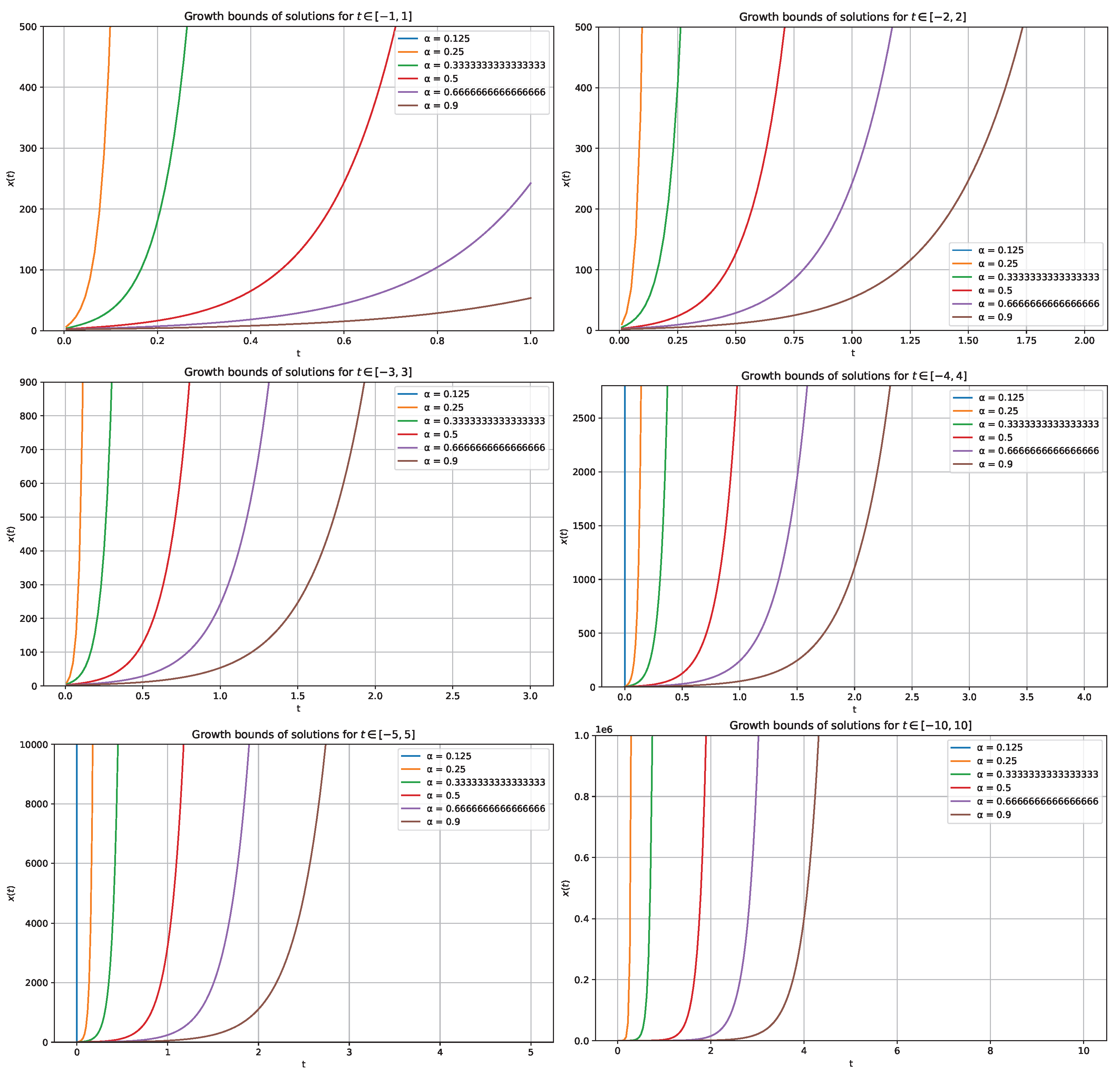
The plots in Figure 1 below illustrate the growth behaviours and corresponding bounds of the solution for various values of the parameter α over different time intervals. It is observed that the curves become progressively steeper as the time interval increases positively, indicating that the solution exhibits standard exponential growth behavior for all values of α and for all $t\ge 0$. Moreover, as α approaches zero, the solution demonstrates a slower growth rate and, consequently, a larger growth bound. However, for $t\in [-{\tau }^{*},0],{\tau }^{*}>0$, he solution trajectories associated with different values of α tend to exhibit zero exponential growth or remains constant over the history interval. This indicates that the system exhibits no growth over the initial history interval, as the solution is completely determined by the prescribed history function on $[-{\tau }^{*},0]$.

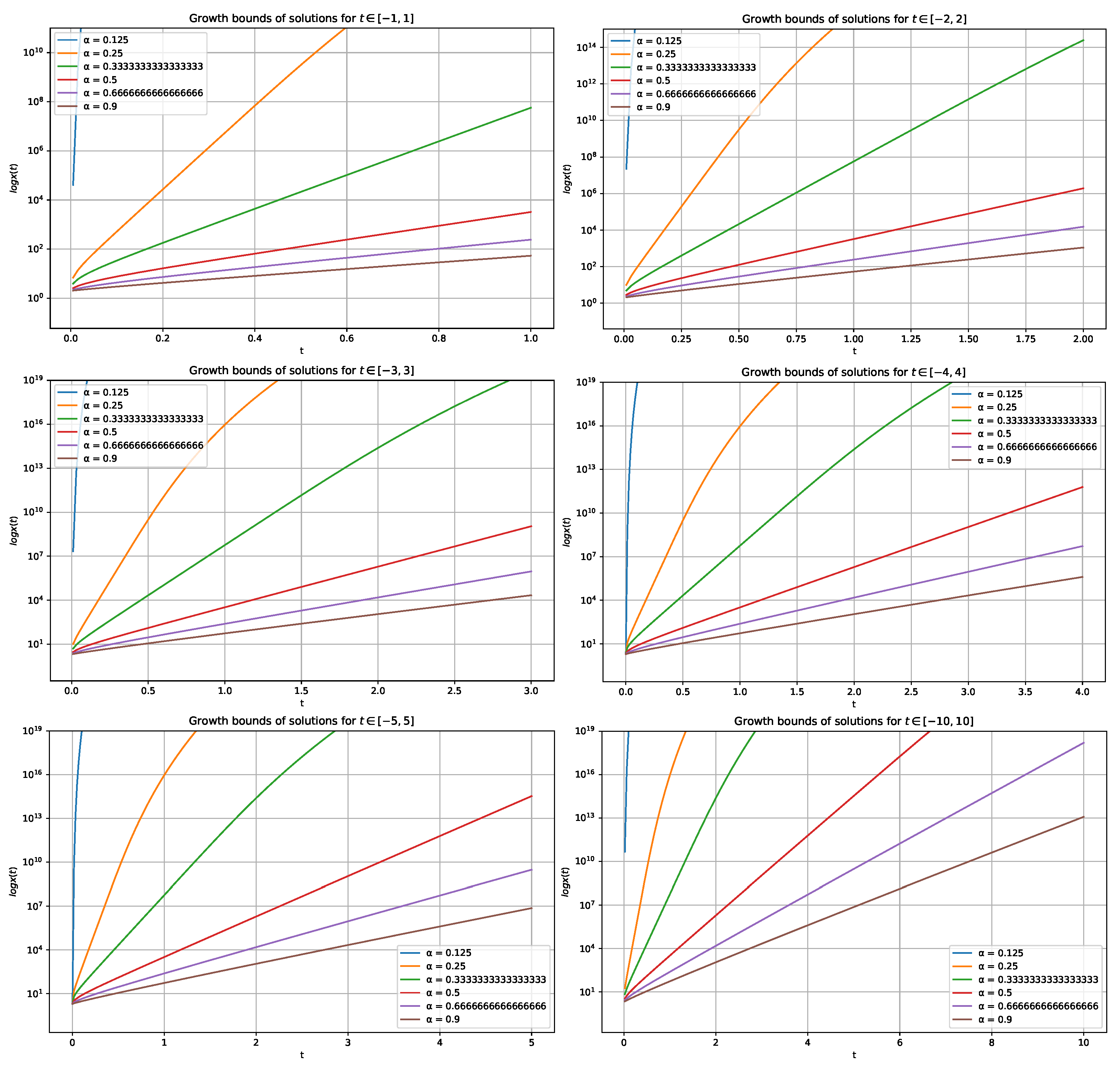
To clearly visualize and better illustrate the growth bounds of each solution, the logarithm (of the absolute value) of the solution function is plotted in Figure 2, as shown below.

An interesting insight is to investigate the effect of varying the Lipschitz constants, ${\ell }_f$ and ${\ell }_g$, on the growth behaviour of the solution. Consider for $\alpha ={\displaystyle \frac{2}{3}}$, with other paramters as above to obtain

$$|x(t)|\le \left[2+{\displaystyle \frac{t^{\frac{2}{3}}}{\mathrm{\Gamma }(\frac{5}{3})}}\right]E_{{\displaystyle \frac{2}{3}}}\left[{\displaystyle \frac{\frac{{\ell }_f}{4}+{\ell }_g}{1-(\frac{{\ell }_f}{4}+\frac{{\ell }_g}{4})}}{t}^{{\displaystyle \frac{2}{3}}}\right].$$

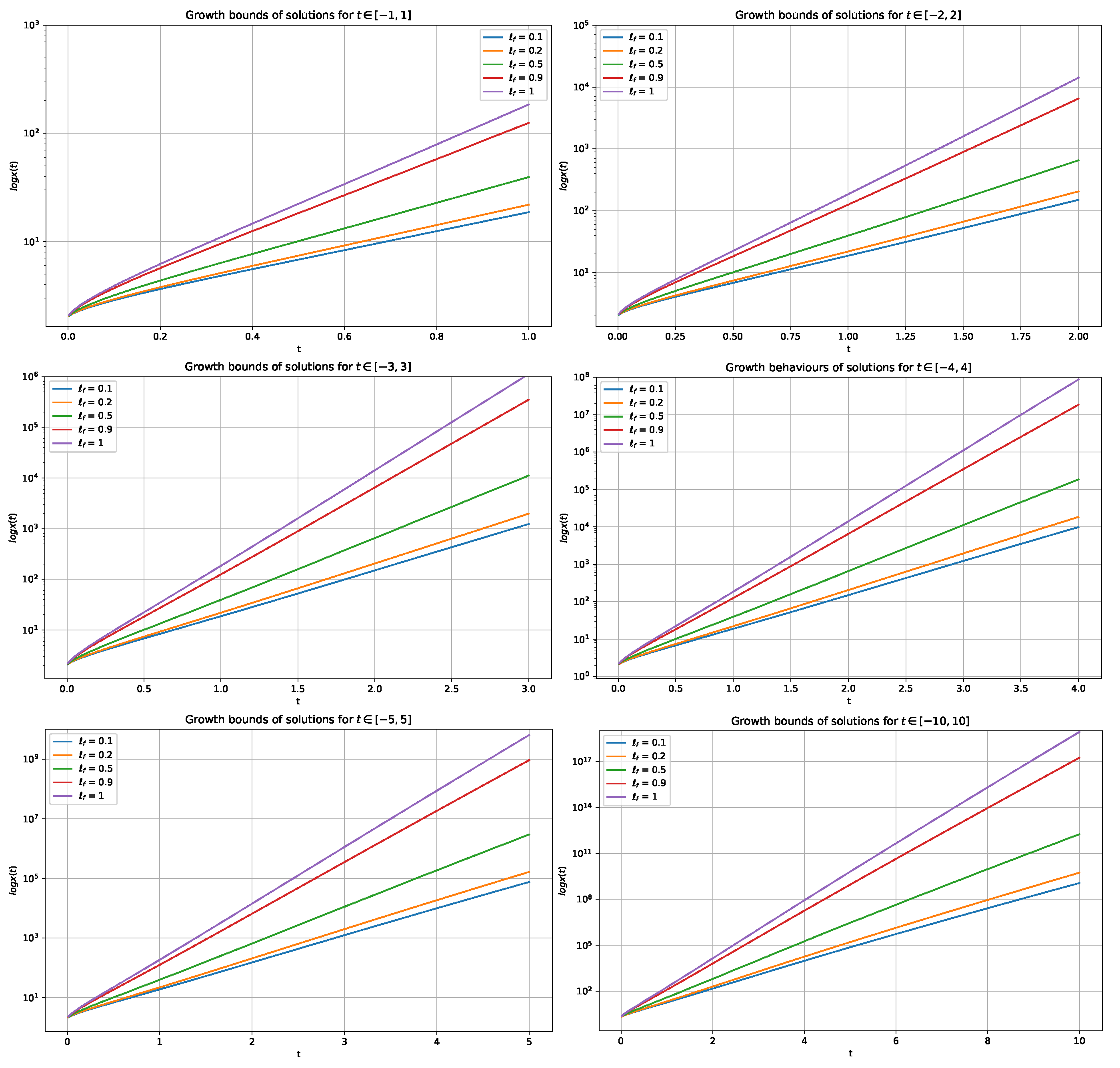
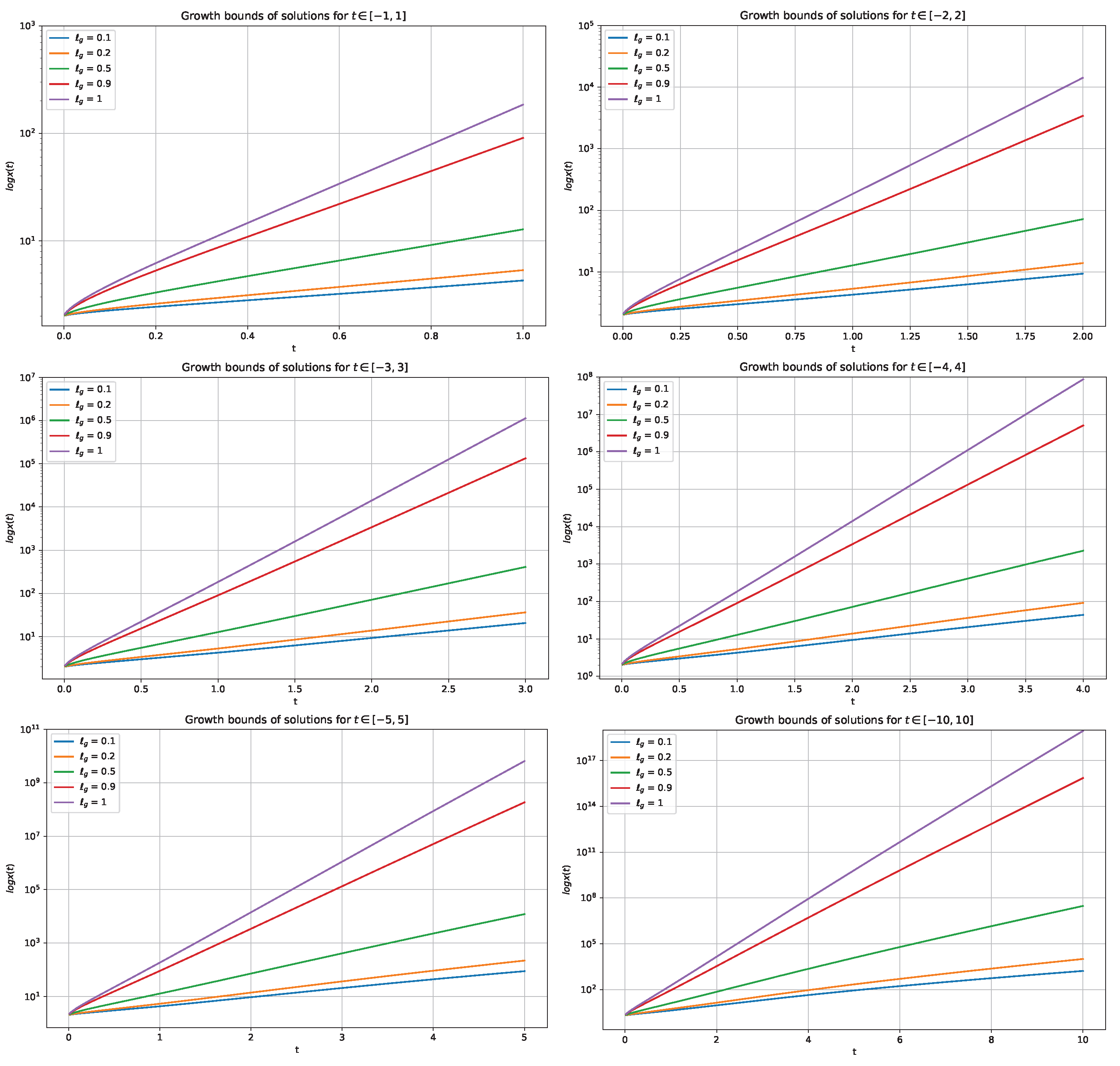
In Figure 3, we fix ${\ell }_f=1$ and vary ${\ell }_g$. Similarly, in Figure 4, we fix ${\ell }_g=1$ and vary ${\ell }_f$. Numerical simulations indicate that changes in these constants have little or no significant influence on the exponential growth behaviour or the corresponding growth bounds of the solution within the parameter ranges considered. See Figure 3 and Figure 4.

5. Conclusions

This research focused on a class of implicit fractional differential equations with state-dependent delay. These equations have applications in modeling real-world phenomena in control theory, biology and medicine, and economics and finance. They have the ability of simultaneously capturing memory, hereditary, and time-delay effects. The main results cover the existence and uniqueness of solution and an exponential growth bound. For future research or open problem, one could consider the problem for an implicitly defined delay $\tau (x(t-\tau ))$ where the state at the initiating event determines the duration of the delay. Furthermore, one could also consider the more general model $\tau (x(t),x(t-\tau )),$ as well as extending the approach developed by the authors in [18] to our present work. Another promising direction is to generalize the model to incorporate multiple state-dependent delays or fractional derivatives of different orders. Finally, it would be worthwhile to investigate the continuous dependence of solutions on the state-dependent delay function and the prescribed history, establish Ulam–Hyers stability, and study the long-term asymptotic behaviour and other qualitative properties of the solution.

References

1. Bhalekar, S.; Gupta, D. Stability and bifurcation analysis of a fractional order differential equation involving cubic nonlinearity. Chaos Solitons Fractal 2022, 162, 112483. [Google Scholar] [CrossRef]
2. Bhalekar, S.; Dutta, P. Analysis of a class of two-delay fractional differential equation. Chaos An. Interdiscip. J. Nonlinear Sci. 2025, 35, 013155. [Google Scholar] [CrossRef]
3. Debbouche, A.; Torres, D.F.M. Approximate controllability of fractional nonlocal delay semilinear systems in Hilbert Spaces. Int. J. Control 2013, 86, 1577–1585. [Google Scholar] [CrossRef]
4. Darwish, M.A.; Ntouyas, S.K. Functional differential equations of Fractional order with state-dependent delay. Dyn. Syst. Appl. 2009, 18, 539–550. [Google Scholar]
5. Benchohra, M.; Berhoun, F. Impulsive fractional differential equations with state-dependent delay. Commun. Appl. Anal. 2010, 14, 213–224. [Google Scholar]
6. Belmekki, M.; Mekhalfi, K. On fractional differential equations with state-dependent delay via Kuratowski Measure of Noncompactness. Filomat 2017, 31, 451–460. [Google Scholar] [CrossRef]
7. Chahdane, H.; Khennouf, S. Existence Results for Fractional Integro-differential Equations (FRIDE) with state-dependent delays and infinite delay in Frechet spaces. J. Comput. Anal. Appl. 2024, 33, 1254–1266. [Google Scholar]
8. Damag, F.H.; Qurtam, A.A.; Ali, A.; Elsayed, A.; Adam, A.; Aldwoah, K.; Ali, S.O. Fractal–Fractional coupled systems with constant and state-dependent delays: Existence Theory and Ecological Applications. Fractal Fract. 2025, 9, 652. [Google Scholar] [CrossRef]
9. Pradeepa, R.; Jayaraman, R. Controllability of fractional stochastic neutral integro-differential equations with state-dependent delay in Frechet spaces. Trans. Theor. Math. Phys. 2025, 2, 54–65. [Google Scholar]
10. dos Santos, J.P.C.; Cuevas, C.; Andrade, B. Existence results for a fractional equation with state-dependent delay. Adv. Differ. Equ. 2011, 2011, 642013. [Google Scholar] [CrossRef]
11. dos Santos, J.P.C.; Arjunan, M.M.; Cuevas, C. Existence results for fractional neutral integro-differential equations with state-dependent delay. Comput. Math. With Appl. 2011, 62, 1275–1283. [Google Scholar] [CrossRef]
12. Baleg, M.; Ghezal, A. Theoretical analysis and applications of fixed-point theorems in delay fractional differential equations. J. Appl. Math. Comput. 2025, 71, 867–881. [Google Scholar] [CrossRef]
13. Arthur, G.; Vaanmathi, M.; Ma, Y.-K. Controllability of Stochastic fractional systems involving state-dependent delay and impulsive effects. Adv. Contin. Discret. Model. 2024, 2024, 4. [Google Scholar] [CrossRef]
14. Liang, Y.; Fan, Z.; Li, G. Existence, Uniqueness and Regularity of Solutions for fractional integro-differential equations with state-dependent delay. J. Appl. Anal. Comput. 2023, 14, 623–641. [Google Scholar]
15. Benchohra, M.; Litimein, S.; N’Guerekata, G. On fractional integro-differential inclusion with state-dependent delay in Banach space. Appl. Anal. 2011, 92, 335–350. [Google Scholar] [CrossRef]
16. Mahmudov, N.I. Relative controllability of linear state-delay fractional systems. Fract. Calc. Appl. Anal. 2024, 27, 987–1016. [Google Scholar] [CrossRef]
17. Wang, F.F.; Chen, D.Y.; Zhang, X.G.; Wu, Y. The existence and uniqueness theorem of the solution to a class of nonlinear fractional order system with time delay. Appl. Math. Lett. 2016, 53, 45–51. [Google Scholar] [CrossRef]
18. Vivek, D.; Sunmitha, S.; Elsayed, E.M. Studies on convergence and stability of iterative learning control in impulsive fractional systems with Hilfer fractional derivative. Calcolo 2026, 63, 2. [Google Scholar]
Figure 1. Growth Behaviours of the solution for various values of t and parameter α .
Fractalfract 10 00503 g001
Figure 2. Growth Behaviours of the l o g of solution for various values of t and parameter α .
Fractalfract 10 00503 g002
Figure 3. Growth Behaviours of the l o g of solution for various values of t and Lipschitz constant f .
Fractalfract 10 00503 g003
Figure 4. Growth Behaviours of the l o g of solution for various values of t and Lipschitz constant g .
Fractalfract 10 00503 g004
Disclaimer/Publisher’s Note: The statements, opinions and data contained in all publications are solely those of the individual author(s) and contributor(s) and not of MDPI and/or the editor(s). MDPI and/or the editor(s) disclaim responsibility for any injury to people or property resulting from any ideas, methods, instructions or products referred to in the content.