Construction and Parameter Identification of Two-Dimensional Coupled Fractional-Order Dynamic Model for LCOPA

Abstract

Aiming at the limitation that the traditional integer-order dynamic model of a liquid crystal optical phased array (LCOPA) cannot simultaneously characterize the liquid crystal deformation memory effect, cross-coupling of two-dimensional deflection channels and time-delay characteristics, this paper proposes a two-dimensional coupled fractional-order dynamic modeling and parameter identification method based on fractional calculus. First, the two-dimensional beam deflection mechanism of LCOPA is analyzed to establish a static beam propagation model. Then, a fractional-order generalized Kelvin constitutive equation is adopted to construct a coupled dynamic model integrating multi-element coupling, channel cross-coupling and time-delay characteristics. A Legendre wavelet integral operational matrix is constructed to simplify fractional operations, combined with the least squares algorithm to achieve synchronous high-precision identification of multiple parameters. Finally, an experimental platform is built for verification. The results show that the proposed model achieves a fitting degree of 98% for beam deflection dynamics, with steady-state prediction error less than 0.15% and dynamic RMSE no more than 0.00020 rad, significantly outperforming integer-order models. This research provides theoretical support and engineering reference for modeling and controller design of high-precision non-mechanical beam steering systems.

1. Introduction

A liquid crystal optical phased array (LCOPA) is an electro-optic modulation device capable of achieving non-mechanical beam deflection [1,2,3]. Featuring small size, light weight, low power consumption, and high flexibility [4,5,6], it effectively overcomes the limitations of traditional mechanical rotating components, including slow deflection speed, low pointing accuracy, complex control systems, beam jitter, and difficulty in miniaturization and lightweight design [7,8]. At present, optical phased arrays have become a cutting-edge research hotspot in the field of laser regulation. Among various types of optical phased arrays, liquid crystals have been widely applied due to their excellent dielectric anisotropy and electro-optic birefringence characteristics [9,10]. In LCOPA, liquid crystal molecules are coupled with each other. The synchronous out-of-phase regulation of multiple elements induces viscoelastic coupled deformation of liquid crystal molecules, forming diverse molecular arrangements and enabling high-precision and agile beam pointing. It has broad application prospects in fields such as laser radar [11,12,13], free-space optical communication [14,15], adaptive optics [16], and beam shaping [17,18].

However, the two-dimensional beam deflection performance of LCOPA is restricted by multiple factors, and three core challenges remain in practical applications. First, the viscoelastic properties of liquid crystal molecules endow their dynamic response with fractional-order characteristics, making it difficult for traditional integer-order models to accurately describe the deflection dynamic process [19]. Second, the spatial overlap of liquid crystal molecules and electrode mutual interference between the horizontal and pitch channels lead to significant cross-coupling effects, which destroy the independence of single-channel deflection and degrade the deflection accuracy. Third, fractional-order models contain fractional-order integral terms with high computational complexity, making it difficult to achieve high-precision parameter identification through traditional methods, which further limits the improvement of deflection control accuracy [20].

At present, scholars at home and abroad have conducted extensive research on beam deflection modeling of LCOPA. Based on the Oseen–Frank equation and Ericksen–Leslie equation, studies [21,22] describe the entire dynamic evolution process of the equilibrium orientation distribution of liquid crystal molecules under external field stabilization and their orientation dynamic behavior under electric field action and a model between driving voltage and liquid crystal response time through numerical analysis has been established [23]. Ref. [24] uses exponential function fitting to describe the relaxation process of liquid crystals. Ref. [25] establishes a wave control model of LCOPA based on blazed grating theory and the Fraunhofer propagation principle, but this method can only obtain the corresponding relationship between beam control angle and steady-state phase delay and cannot characterize the dynamic change of far-field spot angle. Lin et al. [26] acquire light intensity image sequences using a high-speed CCD camera and resolve the spot centroid, then establish an integer-order dynamic model combined with a first-order inertial link to describe the dynamic response of LCOPA. However, they ignore the fractional-order viscoelastic characteristics of liquid crystal molecules, resulting in limited model accuracy. Li Lanting [27] establishes a relaxation model of LCOPA by analyzing its equivalent circuit model, builds a beam deflection experimental platform to accurately measure the beam deflection angle, and solves the parameters of the beam deflection system relaxation model using the least squares method. Ref. [28] starts from the deformation characteristics of liquid crystals, constructs a fractional-order beam deflection model of LCOPA through fractional calculus theory, and solves the unknown parameters of the model combined with system identification methods. This makes the fractional-order model more accurately match the characteristics of the actual system and obtain a more accurate system description, but it does not consider inter-channel coupling effects and deviates from the actual device characteristics. Zhang Y, et al. [29] conducted an in-depth analysis of the dynamic response characteristics and far-field diffraction model of the liquid crystal optical phased array. By investigating the beam deflection characteristics during the dynamic response process, they provided a theoretical foundation for high-precision beam deflection control.

In summary, existing studies mostly focus on one-dimensional deflection models of LCOPA, failing to fully consider the cross-coupling effect between azimuth and pitch angles under actual working conditions. Most models are established based on a single element, either integer-order or fractional-order, and cannot comprehensively characterize the coupling influence of multi-element cooperative operation. To address these key challenges, including the difficulty of integer-order models in describing the viscoelastic memory characteristics of liquid crystals, the difficulty in accurate modeling of two-dimensional channel coupling, and the complexity of fractional-order parameter identification, this paper systematically conducts research on two-dimensional coupled fractional-order dynamic modeling and parameter identification. First, the two-dimensional beam deflection mechanism under multi-element cooperation is revealed, a static propagation model based on the radar phased array principle is established, and the quantitative mapping relationship between deflection angles and electrode phase differences is clarified. On this basis, combined with fractional calculus and the generalized Kelvin constitutive equation, a two-dimensional fractional-order dynamic model that simultaneously accounts for multi-element coupling, channel cross-coupling, and time delay is constructed for the first time, effectively solving the problem of limited accuracy of integer-order models. Furthermore, an identification method based on the Legendre wavelet integral operational matrix is proposed, which converts fractional-order operations into pure algebraic operations and achieves synchronous high-precision identification of model order, coefficients, and time delay. Finally, the effectiveness of the proposed two-dimensional coupled fractional-order dynamic model construction and parameter identification method for LCOPA is verified through experiments. The research results provide theoretical support and engineering reference for high-precision non-mechanical beam steering systems and have important engineering application value.

2. Two-Dimensional Beam Deflection Method Based on LCOPA

2.1. LCOPA Beam Deflection Method Based on Radar Phased Array Principle

Based on the Huygens–Fresnel principle, the secondary wavelets from each point on the wavefront undergo coherent superposition in the far field, jointly determining the propagation direction and the intensity distribution of the light beam. For an observation point $P$, the complex amplitude produced by a continuous wavefront $\Sigma$ can be expressed as:

$$E\left(P\right)=K{\displaystyle {\iint }_{\Sigma }F}\left({\theta }_0,\theta \right)E_0(Q){\displaystyle \frac{\exp (jkr)}{r}}d\Sigma$$

(1)

where $d\Sigma$ is the wavefront surface element, $E_0(Q)$ is the initial amplitude of the secondary source, ${\displaystyle \frac{\exp (jkr)}{r}}$ is the phase and amplitude attenuation term of spherical wave propagation, $F({\theta }_0,\theta )$ is the obliquity factor, and $K$ is a proportionality constant.

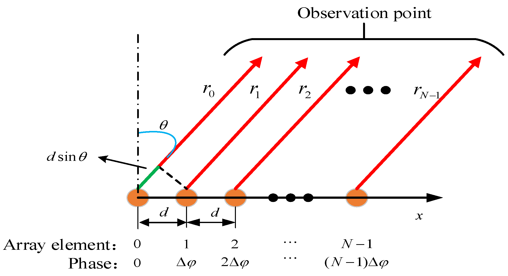
For the discrete electrode structure of the LCOPA, by discretizing the continuous wavefront integral into the coherent superposition of $N$ equally spaced array elements, the far-field complex amplitude expression for a linear array LCOPA can be obtained. The structure of the $N$-dimensional uniform LCOPA is shown in Figure 1, with an element spacing of $d$.

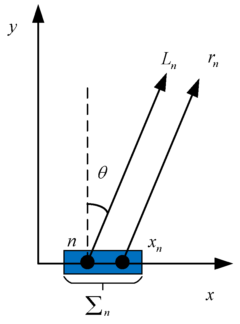
If we consider the $n$-th array element individually, its radiation source model and coordinate relationship are shown in Figure 2. In the figure, ${\Sigma }_n$ denotes the equivalent radiation surface of the $n$-th array element, $x_n$ is the position coordinate of this array element in the $x$-direction, $L_n$ is the reference distance, and $r_n$ is the actual propagation distance from the $n$-th array element to the observation point $P$.

From the geometric relationship in Figure 2, we obtain: $r_n=L_n-x_n\sin \theta$. Substituting this path difference relation into Equation (1) and performing a discrete summation over the $N$ array elements yields the far-field complex amplitude expression for the one-dimensional linear-array LCOPA:

$$E(\theta )={\displaystyle \sum _{n=0}^{N-1}{A}_n}\exp (j{\phi }_n)\exp (-jk{r}_n)$$

(2)

where $A_n$ is the amplitude of the radiation source and ${\phi }_n$ is the phase of the radiation source.

Neglecting the amplitude differences among different array elements and the influence of the constant phase term $\exp (-jk{r}_n)$, we obtain:

$$E(\theta )={\displaystyle \sum _{n=0}^{N-1}{A}_n}\exp (j{\phi }_n)\exp (-jknd\sin \theta )$$

(3)

Setting the phase difference between adjacent phased array elements as $\Delta \phi$, i.e., ${\phi }_n=n\Delta \phi$, and substituting this into Equation (3), then summing and simplifying the arithmetic phase sequence, the normalized far-field intensity distribution can be obtained as:

$$\left|E_n(\theta )\right|={\displaystyle \frac{1}{N}}\left|{\displaystyle \frac{\sin \frac{kNd(\sin {\theta }_s-\sin \theta )}{2}}{\sin \frac{kd(\sin {\theta }_s-\sin \theta )}{2}}}\right|$$

(4)

When $\theta ={\theta }_s$, the intensity reaches its main-lobe maximum, and at this time the phase difference and the beam deflection angle satisfy the following mapping relation:

$$\sin {\theta }_s={\displaystyle \frac{\lambda }{2\pi d}}\Delta \varphi$$

(5)

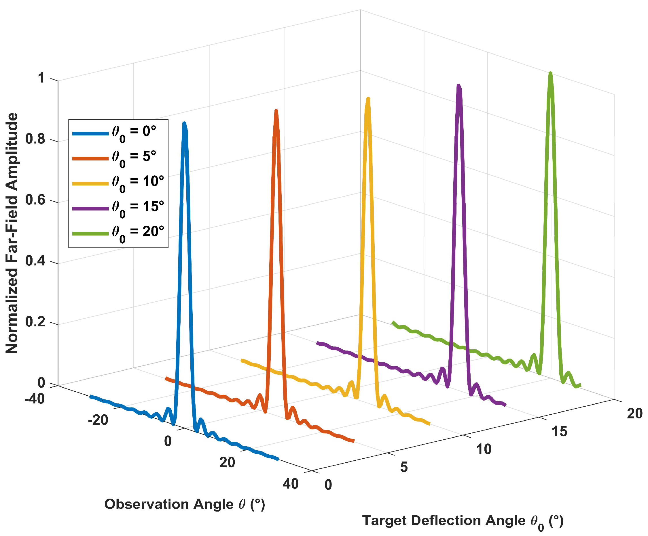
Equation (5) describes the fundamental steering law of the LCOPA beam. It can be seen that the pointing angle of the far-field main lobe can be continuously adjusted by controlling the phase difference $\Delta \phi$ between adjacent array elements. In this work, the incident wavelength of the liquid crystal optical phased array is set to 1064 nm, the number of array elements $N=32$, and the element spacing $d=1.2\lambda$. The selected element spacing reflects the current manufacturing level of LCOPA devices. Ideally, grating lobes can be completely eliminated when $d<\lambda /2$, yet this ideal condition cannot be realized with current fabrication techniques due to engineering limitations including electrode lithography precision and wiring density. Therefore, $d=1.2\lambda$ is adopted as a compromise parameter balancing theoretical performance and practical manufacturability. Under this structural parameter, grating lobes inevitably exist, but they only redistribute the output optical energy without shifting the spatial pointing of the main lobe. Moreover, the system proposed in this paper only operates within a tiny deflection range of $0~10°$, where our research focuses on the static pointing accuracy and dynamic deflection evolution of the main lobe [30]. Within such small-angle working conditions, the peak intensity of side lobes induced by high-order diffraction components is far lower than that of the main lobe. Neither grating lobes nor high-order diffraction side lobes spatially overlap with the target scanning main lobe, and their disturbances to main-lobe position, dynamic response and overall modeling conclusions are negligible [29]. Accordingly, only the dominant 0-th diffraction order is retained in the subsequent derivation of diffraction integrals to realize simplified modeling. Optical field simulations are carried out with the above parameters, and the results are presented in Figure 3.

The simulation results show that the LCOPA can achieve precise beam pointing within the target deflection range of $0~20°$, and the far-field main lobe corresponding to each target deflection angle can be accurately focused at the preset angle, verifying the effective regulation of the far-field intensity distribution by phase modulation under ideal conditions.

2.2. Construction of Two-Dimensional Beam Propagation Model for LCOPA

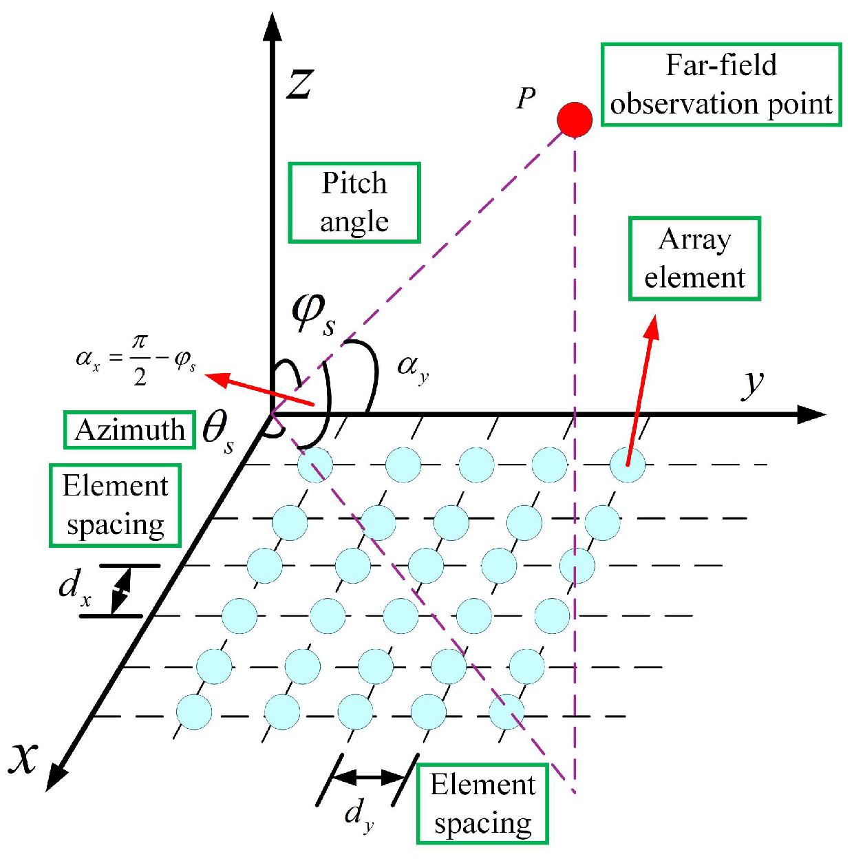
Combining the derivation of one-dimensional LCOPA beam deflection in Section 2.1, and considering that two mutually perpendicular one-dimensional LCOPAs are combined to form a planar LCOPA surface, a liquid-crystal-based two-dimensional beam propagation model can be established, as shown in Figure 4 below. Its radiation sources are arranged in a two-dimensional array. The light emitted by each radiation source in the two-dimensional array also interferes in the far field, ultimately forming a scanning beam. This matrix-array optical phased array can steer the beam in two directions.

In Figure 4 above, the element spacing in the $x$-direction is $d_x$, with a total number of elements $M$; the element spacing in the $y$-direction is $d_y$, with a total number of elements $N$. Taking the element at the origin as the reference element, the spatial coordinates of any element numbered $(m,n)$ are $(m{d}_x,n{d}_y)$. When the beam emitted by this element reaches the far-field observation point $P(\theta ,\phi )$, the optical path difference relative to the reference element is formed by the superposition of the spatial offsets in the two orthogonal directions $x$ and $y$. The geometric optical path difference expression is:

$$L_{mn}=L_0-(m{d}_x\sin \theta \cos \phi +n{d}_y\sin \theta \sin \phi )$$

(6)

where $\theta$ represents the pitch scanning angle, and $\phi$ represents the azimuth scanning angle; $m=0,1,2,\dots M-1$, and $n=0,1,2,\dots N-1$.

This formula is a direct extension of the one-dimensional optical path difference formula to multiple dimensions, indicating that the optical path difference from any array element in the two-dimensional array to the far-field observation point can be decomposed into the sum of the optical path difference in the $x$-direction and that in the $y$-direction, providing the geometric basis for two-dimensional far-field superposition.

If a driving phase ${\phi }_{mn}$ can be independently applied to each array element, the light propagation process will introduce a phase delay term $\exp (-jk{L}_{mn})$. The radiated optical fields from all array elements undergo coherent superposition in the far field; therefore, the total complex amplitude of the two-dimensional array at the far-field observation point $P(\theta ,\phi )$ can be expressed as:

$$E(\theta ,\phi )={\displaystyle \sum _{m=0}^{M-1}{\displaystyle \sum _{n=0}^{N-1}{A}_{mn}}}\exp (j{\phi }_{mn})\exp (-jk{L}_{mn})$$

(7)

Substituting Equation (6) into Equation (7), we obtain:

$$\begin{array}{ll}E(\theta ,\phi )& ={\displaystyle \sum _{m=0}^{M-1}{\displaystyle \sum _{n=0}^{N-1}{A}_{mn}}}\exp [j{\phi }_{mn}]\exp \{-jk[L_0-(m{d}_x\sin \theta \cos \phi +n{d}_y\sin \theta \sin \phi )]\}\\ & ={\displaystyle \sum _{m=0}^{M-1}{\displaystyle \sum _{n=0}^{N-1}{A}_{mn}}}\exp [j{\phi }_{mn}]\exp (-jk{L}_0)\cdot \exp [jk(m{d}_x\sin \theta \cos \phi +n{d}_y\sin \theta \sin \phi )]\end{array}$$

(8)

The term $\exp (-\mathrm{j}k{L}_0)$ only contains the fixed reference optical path $L_0$. This phase factor does not involve the row and column indices m, n of the array and remains constant regardless of the position of any array element. It acts as a global constant phase and can be factored out of the double summation. Thus, Equation (8) can be rewritten as:

$$\begin{array}{ll}E(\theta ,\phi )& ={\displaystyle \sum _{m=0}^{M-1}{\displaystyle \sum _{n=0}^{N-1}{A}_{mn}}}\exp [j{\phi }_{mn}]\exp \{-jk[L_0-(m{d}_x\sin \theta \cos \phi +n{d}_y\sin \theta \sin \phi )]\}\\ & =\exp (-jk{L}_0)\cdot {\displaystyle \sum _{m=0}^{M-1}{\displaystyle \sum _{n=0}^{N-1}{A}_{mn}}}\exp [j{\phi }_{mn}]\exp [jk(m{d}_x\sin \theta \cos \phi +n{d}_y\sin \theta \sin \phi )]\end{array}$$

(9)

Beam deflection angle, main-lobe position and side-lobe distribution are solely determined by the relative phase differences between array elements. The term $\exp (-\mathrm{j}k{L}_0)$ exerts no influence on the relative phase differences among distinct elements. Therefore, this constant term can be directly omitted during the derivation of far-field complex amplitude, and Equation (9) can be further simplified as:

$$E(\theta ,\phi )={\displaystyle \sum _{m=0}^{M-1}{\displaystyle \sum _{n=0}^{N-1}{A}_{mn}}}\exp [j{\phi }_{mn}]\exp [-jk(m{d}_x\sin \theta \cos \phi +n{d}_y\sin \theta \sin \phi )]$$

(10)

In the formula, $A_{mn}$ denotes the output optical amplitude of the $(m,n)$-th array element, the wave number is defined as $k=2\pi /\lambda$, and ${\phi }_{mn}$ represents the electrically controlled phase loaded on the array element.

To simplify the solution of the two-dimensional optical field, this section adopts the ideal assumption that the $x$ and $y$ channels are mutually independent: the electric field crosstalk caused by the spatial overlap of electrodes is neglected, and the driving phases of the two dimensions do not affect each other. In this case, the total phase of the array element can be decomposed into the sum of the independent phases of the two dimensions:

$${\phi }_{mn}=m\Delta {\phi }_x+n\Delta {\phi }_y$$

(11)

where $\Delta {\phi }_x$ and $\Delta {\phi }_y$ are the phase differences between adjacent array elements in the $x$- and $y$-directions, respectively.

For an ideal LCOPA, all array elements emit uniform light intensity, i.e., $A_{mn}=A_0$. The constant amplitude term can be factored out of the summation operators to simplify calculation. Substitute Equation (11) into Equation (10); the exponential term can be decomposed into the product of two independent exponential functions corresponding to the $x$ and $y$ axes, and the double summation is further separated into the product of two one-dimensional summations. The complete transformation procedure is given as follows:

$$\begin{array}{ll}E(\theta ,\phi )& ={\displaystyle \sum _{m=0}^{M-1}{\displaystyle \sum _{n=0}^{N-1}{A}_{mn}}}\exp [j(m\Delta {\phi }_x+n\Delta {\phi }_y)]\exp [-jk(m{d}_x\sin \theta \cos \phi +n{d}_y\sin \theta \sin \phi )]\\ & ={\displaystyle \sum _{m=0}^{M-1}{\displaystyle \sum _{n=0}^{N-1}{A}_{mn}}}\exp [jm\Delta {\phi }_x]·\exp [jn\Delta {\phi }_y]·\exp [-jk(m{d}_x\sin \theta \cos \phi )]·\exp [-jk(n{d}_y\sin \theta \sin \phi )]\\ & =A_0{\displaystyle \sum _{m=0}^{M-1}{\displaystyle \sum _{n=0}^{N-1}\exp [jm\Delta {\phi }_x]\exp [-jk(m{d}_x\sin \theta \cos \phi )]·\exp [jn\Delta {\phi }_y]\exp [-jk(n{d}_y\sin \theta \sin \phi )]}}\\ & =A_0{\displaystyle \sum _{m=0}^{M-1}{\displaystyle \sum _{n=0}^{N-1}\exp [jm\Delta {\phi }_x-jk(m{d}_x\sin \theta \cos \phi )]·\exp [jn\Delta {\phi }_y-jk(n{d}_y\sin \theta \sin \phi )]}}\\ & =A_0\left[{\displaystyle \sum _{m=0}^{M-1}\exp }(jm(\Delta {\phi }_x-k{d}_x\sin \theta \cos \phi ))\right]·\left[{\displaystyle \sum _{n=0}^{N-1}\exp }(jn(\Delta {\phi }_y-k{d}_y\sin \theta \sin \phi ))\right]\end{array}$$

(12)

The above Equation (12) shows that the far-field radiation pattern of an ideal uncoupled two-dimensional array is equivalent to the product of the one-dimensional linear array patterns in the $x$- and $y$-directions.

When the main lobe of the beam is precisely aligned with the preset target angle $({\theta }_s,{\phi }_s)$, the two summation terms in the $x$- and $y$-directions simultaneously reach their maxima, and the phase differences within each group are completely canceled. The constraint equations relating the phase differences and the scanning angles in the two dimensions are derived as:

$$\left\{\begin{array}{l}\Delta {\phi }_x={\displaystyle \frac{2\pi d_x}{\lambda }}\sin {\theta }_s\cos {\phi }_s\\ \Delta {\phi }_y={\displaystyle \frac{2\pi d_y}{\lambda }}\sin {\theta }_s\sin {\phi }_s\end{array}\right.$$

(13)

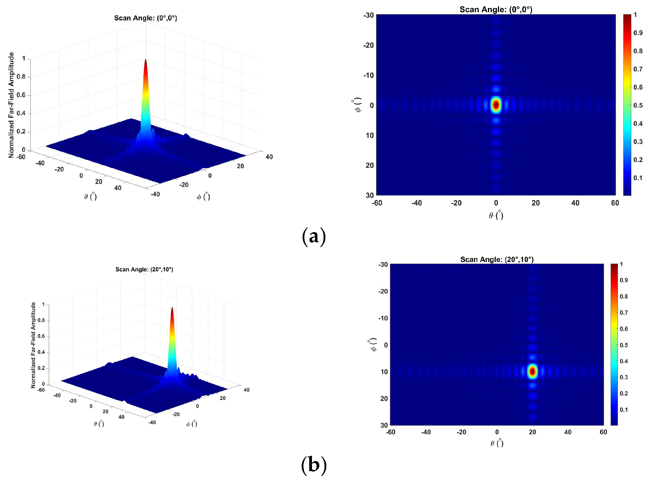
The above Equation (13) shows that the pointing angle of the two-dimensional beam can be uniquely determined by applying phase differences in the $x$- and $y$-directions. The incident wavelength of the liquid crystal optical phased array is set to $1064 \mathrm{nm}$, the element spacing $d$ in both the $x$- and $y$-directions is set to $1.2\lambda$, and the number of array elements is $32\times 32$. Two typical scanning angles, $(0°,0°)$ and $(20°,10°)$, are selected for two-dimensional far-field simulations. The intensity distribution results at different angles are shown in Figure 5.

The simulation results show that, under ideal uncoupled conditions, by independently regulating the electrode phase differences in the two orthogonal directions $x$ and $y$, two-dimensional precise beam pointing can be achieved. The static mapping relationship derived in this section provides static theoretical support for the subsequent two-dimensional fractional-order dynamic model with coupling and time delay.

3. Fractional-Order Characteristics and Coupling Model Construction of LCOPA

The two-dimensional static propagation model derived in Section 2 is established on the ideal assumptions of no crosstalk between the $x$ and $y$ channel electric fields and independent deformation of liquid crystal molecules, clarifying the fundamental mapping relationship between phase difference and deflection angle as well as the operating mechanism of two-dimensional beam deflection in LCOPA. However, in actual LCOPA devices, the electrodes in the $x$- and $y$-directions spatially overlap, the deformations of liquid crystal molecules across multiple array elements are mutually coupled, and there exists non-negligible cross-coupling effects between channels. Therefore, this section takes the proposed two-dimensional static ideal model as the benchmark framework and further introduces multi-element coupled viscoelastic terms, system time-delay characteristics, and inter-channel cross-coupling terms. Combined with the fractional-order generalized Kelvin constitutive equation, a two-dimensional coupled fractional-order dynamic model that better reflects the actual device characteristics is constructed to achieve high-precision control of the far-field beam in LCOPA.

3.1. Fractional-Order Characteristics and Dynamic Constitutive Model of LCOPA

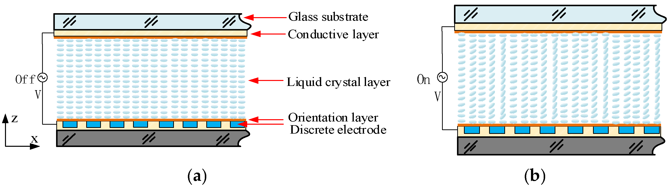
The LCOPA possesses a multi-layer structure, which sequentially consists of cover glass, transparent electrode, alignment layer, liquid crystal layer, reflecting mirror, control electrode array and silicon-based integrated circuit chip from top to bottom. When no driving voltage is applied, liquid crystal molecules align parallel to the cover glass substrate. Under the coordinated driving voltage of multiple array elements, liquid crystal molecules undergo splay, twist and bend deformations. The deformation of liquid crystal manifests as the director vector of liquid crystal molecules tilting toward the direction perpendicular to the glass substrate under the electric field force, i.e., the deflection of liquid crystal molecules. After the external voltage is removed, the liquid crystal molecules recover to the initial state from the current inclined position. Its structural schematic diagram is shown in Figure 6.

The dynamic behavior of the liquid crystal under the action of the electric field force is reflected in the process of the liquid crystal molecules transitioning from one equilibrium state to another, i.e., the liquid crystal undergoes deformation. Since the liquid crystal is viscoelastic, its deformation can be regarded as the simultaneous work of an elastic body and a viscous body. The parameters characterizing the elasticity of the liquid crystal are called elastic coefficients, which can be denoted as $k_1$, $k_2$, and $k_3$ for the splay, twist, and bend elastic coefficients, respectively, according to the deformation characteristics. Similarly, the parameters characterizing the viscosity of the liquid crystal are called viscosity coefficients, denoted as ${\eta }_1$, ${\eta }_2$, and ${\eta }_3$ for the splay, twist, and bend viscosity coefficients, respectively. This deformation process of the liquid crystal is not only related to the current strain rate but also to the historical process of strain, indicating that the deformation possesses history dependence and memory, which conforms to the characteristics of fractional calculus.

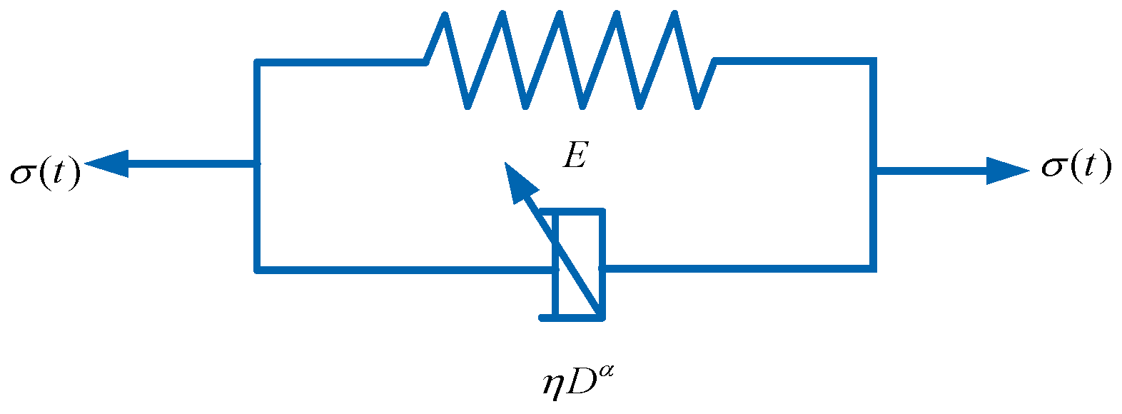
In LCOPA, when multiple array elements work cooperatively, the electric fields of each element spatially overlap. Consequently, the liquid crystal molecular deformation deviates from the ideal deformation under a single element. Affected by adjacent array elements, the liquid crystal of a single element also bears twist deformation and elastic forces generated by deformations of other elements. To characterize such coupled deformation, the Kelvin model, consisting of an elastic element connected in parallel with a viscous element (its structure is shown in Figure 7), can effectively describe this viscoelastic behavior. It is suitable for dynamic modeling of liquid crystal materials under external field excitation and can well reflect the dynamic response of liquid crystal molecules driven by electric fields. Its fractional-order Kelvin viscoelastic model is expressed as:

$$\sigma (t)=E\epsilon (t)+\eta D^{\alpha }\epsilon (t)$$

(14)

where $\sigma (t)$ is the stress, $\epsilon (t)$ is the strain, $E$ is the elastic modulus, $\eta D^{\alpha }\epsilon (t)$ is the fractional-order viscous resistance, $\eta$ is the viscosity coefficient, $D^{\alpha }$ is the fractional-order differential operator, and $\alpha$ is the fractional order. $D^{\alpha }f(t)$ is the Riemann–Liouville fractional derivative, which is defined as [31]:

$$D^{\alpha }f(t)={\displaystyle \frac{1}{\Gamma (n-\alpha )}}{\left({\displaystyle \frac{\mathrm{d}}{\mathrm{d}t}}\right)}^n{\displaystyle {\int }_0^t\frac{f(\tau )}{{(t-\tau )}^{1+\alpha -n}}}\mathrm{d}\tau$$

(15)

where it satisfies $n-1<\alpha <n,n\in \mathbb{N}$, and $\Gamma (\cdot )$ is the Gamma function.

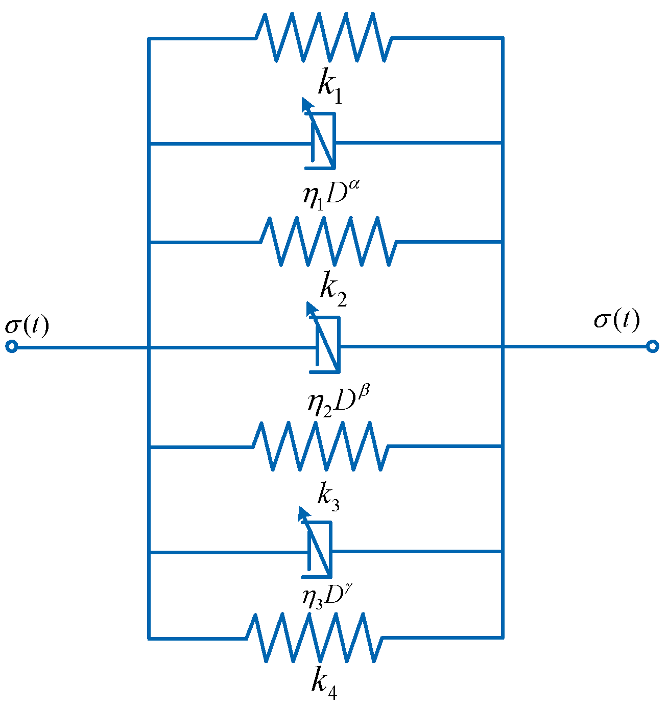
To describe the response behavior of liquid crystals under multi-element coupling during electric field variation, the process can be characterized by a parallel combination of three viscous elements and four elastic elements, forming a fractional-order generalized Kelvin constitutive equation under multi-element coupling. Its structure is illustrated in Figure 8.

Herein, the viscous property corresponding to splay deformation is characterized by the fractional-order viscous element ${\eta }_1{D}^{\alpha }\theta (t)$, the viscous term of twist deformation is ${\eta }_2{D}^{\beta }\theta (t)$, and the viscous term of bend deformation is ${\eta }_3{D}^{\gamma }\theta (t)$. Similarly, the splay elastic effect is described by $k_1\theta (t)$, the twist elastic effect by $k_2\theta (t)$, and the bend elastic effect by $k_3\theta (t)$. The elastic interaction induced by deformation coupling from other adjacent array elements is represented by $k_4\theta (t)$.

Thus, the generalized Kelvin viscoelastic constitutive equation for a single-pixel element of the LCOPA is obtained as follows:

$$F(t)={\eta }_1{D}^{\alpha }\theta (t)+{\eta }_2{D}^{\beta }\theta (t)+{\eta }_3{D}^{\gamma }\theta (t)+k_1\theta (t)+k_2\theta (t)+k_3\theta (t)+k_4\theta (t)$$

(16)

where $\theta (t)$ is the orientation angle of the liquid crystal molecules, and $F(t)$ is the external force applied by the voltage drive; ${\eta }_1,{\eta }_2,{\eta }_3$ are the viscosity coefficients corresponding to splay, twist, and bend deformations, respectively, and $k_1,k_2,k_3$ are the elastic coefficients corresponding to splay, twist, and bend deformations, respectively; $k_4$ characterizes the deformation coupling interaction force between liquid crystal array elements; $\alpha ,\beta ,\gamma$ correspond to the viscous memory intensity orders of splay, twist, and bend deformations, respectively. A higher order indicates that the viscous memory effect of that deformation mode is more significant and the relaxation process is slower. The three deformation modes of the liquid crystal each have independent viscoelastic response mechanisms, and $\alpha ,\beta ,\gamma$ respectively quantify the degree of memory retention of the historical strain history for each mode, reflecting the energy dissipation and recovery characteristics of the internal molecular network of the liquid crystal material during the deformation process.

3.2. Construction of Fractional-Order Coupling Model for LCOPA

Considering that, under multi-element coupling conditions, the spatial overlap of electric fields between adjacent array elements induces twist deformation of liquid crystal molecules, it is necessary to solve the steady-state director distribution of the LCOPA through the principle of free energy minimization. In the free energy solution process, this paper adopts strong anchoring boundary conditions: the orientation of liquid crystal molecules on the surfaces of the upper and lower substrates is fixed by the alignment films, and the surface orientation does not vary with the driving voltage [32].

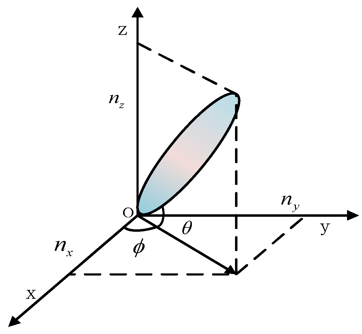
The liquid crystal molecular director $\overrightarrow{n}$ refers to the average alignment direction of the long axes of a large number of liquid crystal molecules per unit volume. In the coordinate system shown in Figure 9, it can be expressed in terms of the tilt angle $\theta$ and the azimuthal angle $\varphi$:

$$\overrightarrow{n}=(\sin \theta \cos \varphi ,\sin \theta \sin \varphi ,\cos \theta )$$

(17)

where $\theta$ and $\varphi$ denote the included angles between the liquid crystal molecular director and the $z$-axis and $x$-axis, respectively.

According to the electro-optic effect of liquid crystals, when a voltage is applied to liquid crystals, the liquid crystal molecules will rotate from their initial stable state to a new equilibrium state. This process can be characterized by the Gibbs free energy density as:

$$f_g={\displaystyle \frac{1}{2}}{k}_1{\left(\nabla \cdot \overrightarrow{n}\right)}^2+{\displaystyle \frac{1}{2}}{k}_2{\left(\overrightarrow{n}\cdot \nabla \times \overrightarrow{n}\right)}^2+{\displaystyle \frac{1}{2}}{k}_3{\left(\overrightarrow{n}\times \nabla \times \overrightarrow{n}\right)}^2$$

(18)

where $k_1=11.1\times {10}^{-12}$ N is the splay elastic constant of liquid crystal, $k_2=7.4\times {10}^{-12}$ N is the twist elastic constant, and $k_3=17.1\times {10}^{-12}$ N is the bend elastic constant. The free energy density corresponding to the electric field is expressed as:

$$f_e={\displaystyle \frac{1}{2}}\left(D\cdot E\right)={\displaystyle \frac{1}{2}}({\epsilon }_{\perp }+\Delta \epsilon {\sin }^2\theta ){\left({\displaystyle \frac{dV}{dz}}\right)}^2$$

(19)

In the above formula, $E$ denotes electric field intensity, $D$ denotes the electric displacement vector, ${\epsilon }_{\perp }=4.6\times {10}^{-11}$ F/m is the perpendicular dielectric constant, and $\Delta \epsilon =1.2\times {10}^{-10}$ F/m is the dielectric anisotropy, $V$ is the external driving voltage.

Within a single array element of LCOPA, the director tilt angle $\theta$ and azimuth angle $\varphi$ are functions of the $z$-axis and $x$-axis with respect to driving voltage $V$, respectively. Combining Equations (17)–(19), the Gibbs free energy density of the system under electric field excitation is derived as:

$$\begin{array}{ll}f& =f_g-f_e\\ & =f\left(\theta ,\varphi \right){\left({\displaystyle \frac{\partial \varphi }{\partial x}}\right)}^2+g\left(\theta \right){\left({\displaystyle \frac{\partial \theta }{\partial z}}\right)}^2+h\left(\theta ,\varphi \right){\displaystyle \frac{\partial \varphi }{\partial x}}{\displaystyle \frac{\partial \theta }{\partial z}}-{\displaystyle \frac{1}{2}}\left({\epsilon }_{\perp }+\Delta \epsilon {\sin }^2\theta \right){\left({\displaystyle \frac{dV}{dz}}\right)}^2\end{array}$$

(20)

Wherein:

$$\begin{array}{l}f\left(\theta ,\varphi \right)={\displaystyle \frac{1}{2}}{\cos }^2\theta \left(k_1{\sin }^2\varphi +k_2{\cos }^2\varphi {\sin }^2\theta +k_{3}co{s}^2\varphi co{s}^2\theta \right)\\ g\left(\theta \right)={\displaystyle \frac{1}{2}}\left(k_1{\cos }^2\theta +k_{3}si{n}^2\theta \right)\\ h\left(\theta ,\varphi \right)=\left(k_2-k_1\right){\cos }^2\theta \sin \varphi \end{array}$$

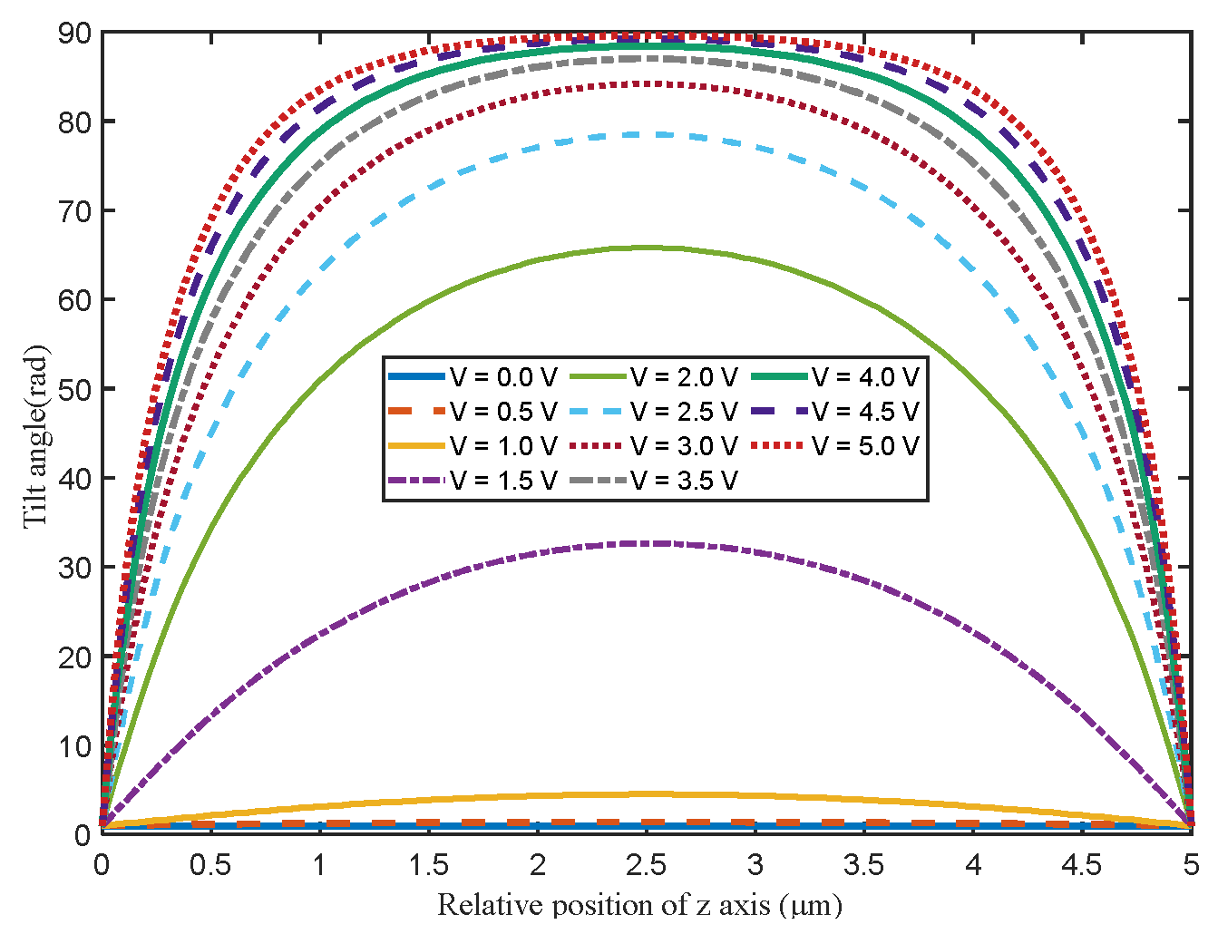
To derive the analytical relationship between tilt angle $\theta$ and driving voltage $V$, variational calculus is performed on the above free energy equation, yielding functional expressions of $\theta$, $\varphi$, and $V$ with respect to the $z$-axis and $x$-axis. The finite difference iterative method is further adopted to solve the spatial distribution of liquid crystal molecular directors, and the final director distribution result is plotted in Figure 10.

It can be observed from the figure that the tilt angles corresponding to liquid crystal directors at different spatial positions exhibit non-linear distribution characteristics. According to linear fractional-order viscoelastic theory, the driving voltage and liquid crystal molecular tilt angle satisfy an approximate linear relation. Thus, $\widehat{\theta }(t)$ is defined as the spatial average value of tilt angles at all positions under the identical driving voltage. Since $\widehat{\theta }(t)$ is the statistical average of tilt angles, the electric field force is also averaged over the cell volume, which gives:

$$F(t)=j{\displaystyle \frac{u(t)}{x}}q$$

(21)

where $q=1.6\times {10}^{-19} \mathrm{C}$ is the elementary charge, $j$ denotes the volume charge distribution coefficient of liquid crystal molecules, $x=9.8 \mathrm{\mu }\mathrm{m}$ is the width of a single array element, and $u(t)$ is the time-varying external driving voltage.

Substitute Equation (21) together with the averaged tilt angle $\widehat{\theta }(t)$ into Equation (16), and the dynamic equilibrium equation of LCOPA is obtained:

$${\displaystyle \frac{jq}{x}}u(t)={\eta }_1{D}^{\alpha }\widehat{\theta }(t)+{\eta }_2{D}^{\beta }\widehat{\theta }(t)+{\eta }_3{D}^{\gamma }\widehat{\theta }(t)+k_1\widehat{\theta }(t)+k_2\widehat{\theta }(t)+k_3\widehat{\theta }(t)+k_4\widehat{\theta }(t)$$

(22)

Based on the two-dimensional beam propagation principle derived in Section 2, two-dimensional beam deflection using liquid crystal optics requires a constant phase gradient along both the azimuth and elevation axes, which means different driving voltages must be applied to adjacent electrodes. Multiple electrodes work cooperatively to achieve a full $2\pi$ phase modulation range. The mapping relation between phase modulation quantity and driving voltage is given by:

$$\Delta \phi =Ku, K=1.257$$

(23)

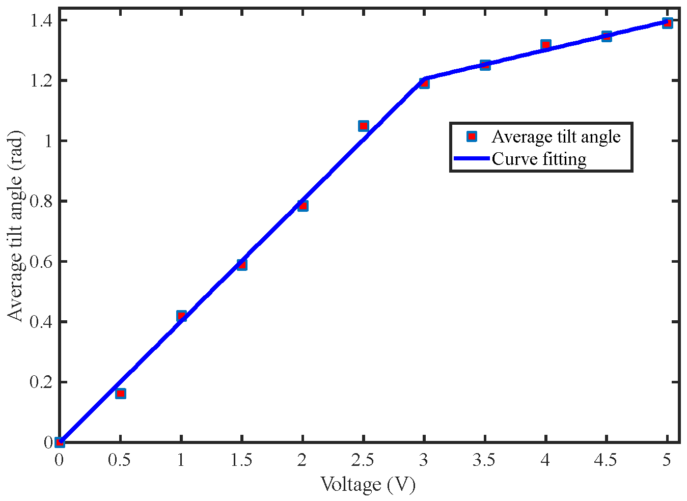
The driving voltage $u$ is correlated not only with the phase modulation quantity but also with the tilt angle of liquid crystal molecules. Based on the numerical results illustrated in Figure 10, a piecewise linear function is utilized to fit the relationship between the driving voltage u and the average tilt angle $\widehat{\theta }$ of liquid crystal molecules. The fitted curve is presented in Figure 11.

According to the fitted results, the relationship between u and $\widehat{\theta }$ can be expressed as:

$$\widehat{\theta }=\left\{\begin{array}{ll}0.4019u& \hspace{1em}0\le u<3\\ 0.095215u+1.2058& \hspace{1em}3\le u\le 5\end{array}\right.$$

(24)

The above Equation (24) describes the spatially averaged orientation angle of liquid crystal molecules under different driving voltages. All values adopted for piecewise fitting are derived from deterministic numerical solutions of the Gibbs free energy model. It is worth emphasizing that the abrupt numerical change at $u=3$ is an inherent objective law of the electric field response of liquid crystal molecules, which is fully validated by complete experimental data. This piecewise fitting function covers the entire operating voltage range of 0~5 V, with a coefficient of determination $R^2>0.995$ and a maximum relative error of the tilt angle less than 1.2%. The fitting accuracy fully meets the requirements of dynamic modeling, and its influence on the final beam pointing accuracy is negligible.

Since the maximum phase difference of the system is $\Delta \phi =\pi$, the corresponding critical voltage is 2.5 V. Substituting the linear fitting relationship corresponding to the 0–−3 V interval in Equation (24) into Equation (23), the mapping relationship between the phase modulation amount and the average tilt angle of the liquid crystal molecules can be derived as:

$$\Delta \phi =Ku={\displaystyle \frac{K}{0.4019}}\widehat{\theta }$$

(25)

Substituting Equation (25) into the continuous modulation governing Equation (5) of LCOPA, the quantitative relation between the beam deflection angle and the average tilt angle of liquid crystal molecules is derived:

$$\widehat{\theta }={\displaystyle \frac{{\theta }_p}{\arcsin (\frac{\lambda }{2\pi d})\times \frac{K}{0.4019}}}$$

(26)

Subsequently, substituting both Equations (25) and (26) into the fractional-order constitutive Equation (22) of the LCOPA, a fractional-order dynamic model linking the beam deflection angle and phase difference is constructed.

$$\begin{array}{l}{\displaystyle \frac{jq}{x}}u(t)={\displaystyle \frac{{\eta }_1}{\arcsin (\frac{\lambda }{2\pi d})\times \frac{K}{0.4019}}}{D}^{\alpha }{\theta }_p(t) +{\displaystyle \frac{{\eta }_2}{\arcsin (\frac{\lambda }{2\pi d})\times \frac{K}{0.4019}}}{D}^{\beta }{\theta }_p(t) \\ \hspace{1em}\hspace{1em}+{\displaystyle \frac{{\eta }_3}{\arcsin (\frac{\lambda }{2\pi d})\times \frac{K}{0.4019}}}{D}^{\gamma }{\theta }_p(t)+{\displaystyle \frac{k}{\arcsin (\frac{\lambda }{2\pi d})\times \frac{K}{0.4019}}}{\theta }_p(t)\\ \arcsin ({\displaystyle \frac{\lambda }{2\pi d}}){\displaystyle \frac{jq}{0.4019x}}△\phi (t) ={\eta }_1{D}^{\alpha }{\theta }_p(t)+{\eta }_2{D}^{\beta }{\theta }_p(t)+{\eta }_3{D}^{\gamma }{\theta }_p(t)+k{\theta }_p(t)\end{array}$$

(27)

In the beam steering system, the data processing and signal transmission stages introduce inherent time delays. It should be noted that the delay parameter $\tau$ here is not a constant but a variable related to the viscoelasticity of the liquid crystal material and the applied electric field. When the operating environment temperature changes significantly, the prediction accuracy of the model may decrease, and in such cases, $\tau$ needs to be recalibrated. Substituting the total system delay $\tau$ into Equation (27), the fractional-order dynamic model for LCOPA beam steering with time delay is finally constructed as:

$$\arcsin ({\displaystyle \frac{\lambda }{2\pi d}}){\displaystyle \frac{jq}{0.4019x}}△\phi (t-\tau ) ={\eta }_1{D}^{\alpha }{\theta }_p(t)+{\eta }_2{D}^{\beta }{\theta }_p(t)+{\eta }_3{D}^{\gamma }{\theta }_p(t)+k{\theta }_p(t)$$

(28)

where the equivalent elastic coefficient satisfies the following relation: $k=k_1+k_2+k_3+k_4.$

Combined with the static beam propagation model derived in the preceding sections, the two-dimensional beam deflection realized by the LCOPA is essentially implemented by manipulating the phase distribution of liquid crystal cells along two orthogonal axes $x$ and $y$, so as to achieve angular deflection of the light beam within the two-dimensional plane. As the final output beam can be equivalently decomposed into the linear superposition of independently deflected beams along the $x$- and $y$-axes, the proposed two-dimensional beam deflection model is essentially a multiple-input multiple-output (MIMO) framework, which accurately characterizes the cooperative interaction mechanism of the LCOPA during two-dimensional beam steering.

Accordingly, for the $x$-axis, applying the fractional-order Laplace transform to Equation (28) yields:

$$G_x(s)e^{-\tau s}={\displaystyle \frac{b_{xx}}{{\eta }_1{s}^{\alpha }+{\eta }_2{s}^{\beta }+{\eta }_3{s}^{\gamma }+k}}{e}^{-{\tau }_{xx}s}$$

(29)

Similarly, for the $y$-axis, the fractional-order Laplace transform is also performed on Equation (28), which gives:

$$G_y(s)e^{-\tau s}={\displaystyle \frac{b_{yy}}{{\eta }_1{s}^{\alpha }+{\eta }_2{s}^{\beta }+{\eta }_3{s}^{\gamma }+k}}{e}^{-{\tau }_{yy}s}$$

(30)

Considering the coupling effects between the two azimuthal axes, independent equivalent time-delay parameters are respectively set for the four transmission paths. Finally, the complete two-dimensional beam deflection model can be expressed in the form of a transfer function matrix:

$$\begin{array}{ll}G(s)=& \left[\begin{array}{cc}{G}_{xx}(s)e^{-{\tau }_{xx}s}& G_{xy}(s)e^{-{\tau }_{xy}s}\\ G_{yx}(s)e^{-{\tau }_{yx}s}& G_{yy}(s)e^{-{\tau }_{yy}s}\end{array}\right]\\ & \left[\begin{array}{cc}{\displaystyle \frac{b_{xx}}{{\eta }_1{s}^{\alpha }+{\eta }_2{s}^{\beta }+{\eta }_3{s}^{\gamma }+k_4}}{e}^{-{\tau }_{xx}s}& {\displaystyle \frac{b_{xy}}{{\eta }_1{s}^{\alpha }+{\eta }_2{s}^{\beta }+{\eta }_3{s}^{\gamma }+k_4}}{e}^{-{\tau }_{xy}s}\\ {\displaystyle \frac{b_{yx}}{{\eta }_1{s}^{\alpha }+{\eta }_2{s}^{\beta }+{\eta }_3{s}^{\gamma }+k_4}}{e}^{-{\tau }_{yx}s}& {\displaystyle \frac{b_{yy}}{{\eta }_1{s}^{\alpha }+{\eta }_2{s}^{\beta }+{\eta }_3{s}^{\gamma }+k_4}}{e}^{-{\tau }_{yy}s}\end{array}\right]\end{array}$$

(31)

4. Parameter Identification of Fractional-Order Time-Delay Systems Based on the Integral Operational Matrix of Legendre Wavelet

In Equation (28), the viscosity coefficients ${\eta }_1$, ${\eta }_2$, ${\eta }_3$ corresponding to splay, twist, and bend deformations of the liquid crystal, the liquid crystal molecular volume-distributed charge coefficient $j$, the fractional orders $\alpha$, $\beta$, $\gamma$, the time-delay constant $\tau$, and the coupling gain coefficients between channels are all unknown parameters to be identified. Therefore, a parameter identification method based on the Legendre wavelet integral operational matrix is introduced. This method utilizes the orthogonality and compact support properties of Legendre wavelet to transform the complex fractional-order time-delay differential equation into a simple algebraic equation and combines it with the least squares method to achieve simultaneous and accurate estimation of model parameters and orders [33].

4.1. Integral Operational Matrix of Legendre Wavelet

The orthogonal polynomials defined on the interval $[-1,1]$ with weight function $\rho (x)=1$ are termed Legendre orthogonal polynomials [34], whose explicit expressions are given by

$$P_0=1,\hspace{1em}{P}_n(t)={\displaystyle \frac{1}{2^{n}n!}}{\displaystyle \frac{{\mathrm{d}}^n}{\mathrm{d}{t}^n}}\left\{{(t^2-1)}^n\right\},\hspace{1em}n=1,2,3,\dots$$

(32)

Legendre polynomials satisfy a recursive relation, and the corresponding recurrence formula is shown as follows:

$$\begin{array}{l}{P}_0(t)=1, P_1(t)=t\\ P_{m+1}(t)=({\displaystyle \frac{2m+1}{m+1}})t{P}_m(t)-({\displaystyle \frac{m}{m+1}})P_m(t)\end{array}$$

(33)

On the interval [0,1], the mother wavelet function can generate a continuous wavelet family via successive translation and scaling transformations, as shown in Equation (34).

$${\psi }_{a,b}(t)={\left|a\right|}^{-1/2}\psi ({\displaystyle \frac{t-b}{a}}), a,b\in \mathit{ℝ}, a\ne 0$$

(34)

In the above expression, the scaling coefficient $a$ and translation coefficient $b$ vary continuously. Discretizing the parameters $a$ and $b$ as $a=a_0^{-k},\hspace{1em}b=n{b}_0{a}_0^{-k},$ yields a family of discrete wavelets.

$${\psi }_{k,n}(t)={\left|a_0\right|}^{k/2}\psi (a_0^{k}t-n{b}_0)$$

(35)

where ${\psi }_{k,n}$ denotes the wavelet basis. Here, $a_0>0$, $b_0>0$, and $n$, $k$ are positive integers.

The following variable substitution is adopted to map the domain of Legendre polynomials to [0,1]:

$$t^{\ast }=2t-1, 0\le t\le 1$$

(36)

Let $P_m(t^{\ast })=P_m(2t-1)$. Combined with Equation (35), we can derive the definition of the Legendre wavelet over the interval [0,1] as follows.

$${\psi }_{k,n}^m(t)= \left\{\begin{array}{cc}\sqrt{m+{\displaystyle \frac{1}{2}}}{2}^{k/2}{P}_m(2^{k}t-\widehat{n}) ,& \hspace{1em}\frac{\widehat{n}-1}{2^k}\le t< \frac{\widehat{n}+1}{2^k} \\ 0& \hspace{1em}\mathrm{otherwise}\end{array}\right.$$

(37)

Here, $k$ is an arbitrary positive integer, $m$ denotes the order of Legendre polynomials with $m=1,2,3,\dots$ and $k=1,2,3,\dots$. The index $\widehat{n}=2n-1$ holds for $n=1,2,3,\dots ,2^{k-1}$, and $t$ represents the normalized time. Different values of $m$ correspond to different Legendre wavelets. Nevertheless, a Legendre wavelet is continuous on the definition interval for any $m$. However, the order of Legendre wavelets increases as $m$ grows. High-order Legendre wavelets will increase the computational cost of parameter identification and reduce the efficiency of system identification. Therefore, to reduce the complexity of parameter identification, Legendre wavelets with $m=1$ are utilized to construct the integral operational matrix.

Define $N=2^k$. Any function $f(t)$ can be expanded by Legendre wavelets as:

$$f(t)=c_{0,0}{\phi }_{0,0}+{\displaystyle \sum _{k=1}^{{\log }_{2}N}{\displaystyle \sum _{n=1}^{2^{k-1}}{c}_{k,n}{\psi }_{k,n}}}=C_N^{\mathrm{T}}{\mathrm{\Phi }}_N(t)$$

(38)

where ${\phi }_{0,0}=1$ is the scaling function, $c_{0,0}$ is the coefficient of the scaling function, and $c_{k,n}=\langle f(t),{\psi }_{k,n}(t)\rangle$ stands for the Legendre wavelet coefficient. The symbol $\langle \cdot ,\cdot \rangle$ denotes the inner product, the superscript $\mathrm{T}$ refers to matrix transposition, and $C_N$, ${\mathrm{\Phi }}_N(t)$ are the Legendre wavelet coefficient matrix and Legendre wavelet matrix, respectively, which are defined as

$$C_N={[c_{0,0},c_{1,1},c_{2,1},c_{2,2},\cdots ,c_{k,2^{k-1}}]}^{\mathrm{T}}$$

(39)

$${\mathrm{\Phi }}_N(t)={[{\phi }_{0,0}(t),{\psi }_{1,1}(t),{\psi }_{2,1}(t),{\psi }_{2,2}(t),\cdots ,{\psi }_{k,2^{k-1}}(t)]}^{\mathrm{T}}$$

(40)

To convert ${\mathrm{\Phi }}_N(t)$ into an $N\times N$ matrix, sampling nodes $t_i$ are introduced, and the values of ${\psi }_{k,n}$ are evaluated at these nodes.

$$t_i={\displaystyle \frac{(2i-1)}{2N}}, i=1,2,3\cdots N$$

(41)

Then the $N\times N$ Legendre wavelet matrix can be expressed as:

$${\mathrm{\Psi }}_{N\times N}=\left[{\mathrm{\Phi }}_N({\displaystyle \frac{1}{2N}}),{\mathrm{\Phi }}_N({\displaystyle \frac{3}{2N}}),\cdots ,{\mathrm{\Phi }}_N({\displaystyle \frac{2N-1}{2N}})\right]$$

(42)

To obtain the integral operational matrix of Legendre wavelets, block pulse functions are introduced. The definition of block pulse functions over the interval $[0,T_f]$ is given by

$${\varphi }_i=\left\{\begin{array}{l}1 {\displaystyle \frac{i-1}{N}}{T}_f<t< {\displaystyle \frac{i}{N}}{T}_f, \\ 0 \mathrm{elsewhere}\end{array}\right.i=1,2,3\cdots N$$

(43)

where $T_f$ denotes the terminal running time of the system. According to Ref. [35], we have

$$(I^{\alpha }{B}_N)(t)=F_{N\times N}^{\alpha }{B}_N(t)$$

(44)

In the above formula, $B_N^{\mathrm{T}}(t)=[{\varphi }_1(t),{\varphi }_2(t),{\varphi }_3(t),\dots ,{\varphi }_N(t)]$ stands for the block pulse basis vector, and $F_{N\times N}^{\alpha }$ represents the fractional integral operational matrix of block pulse functions:

$$F_{N\times N}^{\alpha }={({\displaystyle \frac{T_f}{N}})}^{\alpha }{\displaystyle \frac{1}{\Gamma (\alpha +2)}}{\left[\begin{array}{l}{f}_1 f_2 f_3 \dots f_N \\ 0 f_1 f_2 \cdots f_{N-1} \\ ⋮ \ddots f_1 \cdots f_{N-2} \\ ⋮ \ddots \ddots ⋮ \\ 0 \cdots \cdots 0 f_1\end{array}\right]}_{(N\times N)}$$

(45)

where $f_1=1,f_p=p^{\alpha +1}-2{(p-1)}^{\alpha +1}+{(p-2)}^{\alpha +1},p=2,3,\dots ,N$.

Any integrable function can be expanded in terms of block pulse functions on the prescribed interval $[0,T_f]$ [36]. Thus, the expression of Legendre wavelets in block pulse function form is written as

$${\mathrm{\Phi }}_N(t)={\mathrm{\Psi }}_{N\times N}{B}_N(t)$$

(46)

Combining Equations (44) and (46),

$$(I^{\alpha }{\mathrm{\Phi }}_N)(t)={\mathrm{\Psi }}_{N\times N}{F}_{N\times N}^{\alpha }{B}_N(t)$$

(47)

Suppose the fractional-order integral of the Legendre wavelet matrix ${\mathrm{\Phi }}_N(t)$ is

$$(I^{\alpha }{\mathrm{\Phi }}_N)(t)=P_{N\times N}^{\mathrm{\alpha }}{\mathrm{\Phi }}_N(t)$$

(48)

where $P_{N\times N}^{\alpha }$ is the integral operational matrix of Legendre wavelets. Combining Equations (46)–(48), the expression of $P_{N\times N}^{\alpha }$ can be derived as

$$P_{N\times N}^{\alpha }={\mathrm{\Psi }}_{N\times N}{F}_{N\times N}^{\alpha }{\mathrm{\Psi }}_{N\times N}^{-1}$$

(49)

4.2. Time-Delay Operational Matrix of Legendre Wavelet

The time-delay operational matrix shifts the original operational matrix backward by $\tau$ time units. The time-delay operational matrix of Legendre wavelets can be derived by utilizing the block pulse time-delay function vector $B_N(t-\tau )$.

$$B_N(t-\tau )=E{B}_N(t), t>\tau ,0\le t\le T_f$$

(50)

where $E$ denotes the time-delay matrix of block pulse functions.

The time-delay coefficient $\tau$ can be expressed as:

$$\tau =j_{1}h=j_1{\displaystyle \frac{T_f}{N}}, j_1=1,2,\cdots ,N-1$$

(51)

where $h=T_f/N$ represents the step size of the time-delay matrix.

From Equations (43) and (51), we can obtain

$$\begin{array}{ll}{\varphi }_i(t-\tau )& ={\varphi }_i(t-j_{1}h)\\ & =\left\{\begin{array}{l}1 {\displaystyle \frac{i-1+j_1}{N}}{T}_f\le t<{\displaystyle \frac{i+j_1}{N}}{T}_f\\ 0 \mathrm{elsewhere}\end{array}\right.\\ & ={\varphi }_{i+j_1}(t)\end{array}$$

(52)

Therefore, the block pulse time-delay matrix $E$ can be expanded as:

$$E=\left[\begin{array}{l}0 \cdots 0 1 0 \cdots 0\\ 0 \cdots 0 0 1 \cdots 0\\ ⋮ ⋮ ⋮ ⋮ \ddots ⋮\\ 0 \cdots 0 0 0 \cdots 1\\ 0 \cdots 0 0 0 \cdots 0\\ ⋮ ⋮ ⋮ ⋮ \ddots ⋮\\ 0 \cdots 0 0 0 \cdots 0\end{array}\right]$$

(53)

In Equation (53), the element in the 1st row and $(j_1+1)$-th column of the matrix is $1$; the element in the 2nd row and $(j_1+2)$-th column is $1$, and so on. All the remaining entries of the matrix are $0$.

To derive the time-delay operational matrix of Legendre wavelets, we define ${\mathrm{\Phi }}_N(t-\tau )$ with the following form

$${\mathrm{\Phi }}_N(t-\tau )=Z{\mathrm{\Phi }}_N(t), t>\tau ,0\le t\le T_f$$

(54)

where $Z$ is the time-delay operational matrix of Legendre wavelets.

From Equations (46) and (50), ${\mathrm{\Phi }}_N(t-\tau )$ can be rewritten as

$${\mathrm{\Phi }}_N(t-\tau )={\mathrm{\Psi }}_{N\times N}{B}_N(t-\tau )={\mathrm{\Psi }}_{N\times N}E{B}_N(t)$$

(55)

Combining Equations (47), (54) and (55), we can derive that:

$$Z{\mathrm{\Phi }}_N(t)=Z{\mathrm{\Psi }}_{N\times N}{B}_N(t)={\mathrm{\Psi }}_{N\times N}E{B}_N(t)$$

(56)

Accordingly, the time-delay operational matrix $Z$ of Legendre wavelets can be expressed as

$$Z={\mathrm{\Psi }}_{N\times N}E{\mathrm{\Psi }}_{N\times N}^{-1}$$

(57)

Based on the definition of Riemann–Liouville fractional calculus together with Equations (48) and (54), the time-delay integral operational matrix of Legendre wavelets is derived.

$$(I^{\alpha }{\mathrm{\Phi }}_N)(t-\tau )=Z(I^{\alpha }{\mathrm{\Phi }}_N)(t)=Z{P}_{N\times N}^{\alpha }{\mathrm{\Phi }}_N(t)$$

(58)

4.3. Solution Based on Integral Operational Matrix of Legendre Wavelet

With the integral operational matrix and time-delay integral operational matrix of Legendre wavelets derived, these matrices are adopted to transform the fractional-order model of the LCOPA beam steering system into algebraic equations, which are solved via the least squares method to obtain the identified parameters. Firstly, assume that the fractional differential order $\alpha$ is the highest order in Equation (28). By performing the $\alpha$-order integral on both sides of Equation (28), the fractional-order differential equation can be converted into a fractional-order integral equation.

$$\begin{array}{l}\arcsin ({\displaystyle \frac{\lambda }{2\pi d}}){\displaystyle \frac{jq}{0.4019x}}{I}^{\alpha }\Delta \phi (t-\tau )={\eta }_1{\theta }_p(t)+{\eta }_2{I}^{\alpha -\beta }{\theta }_p(t)\\ \hspace{1em}\hspace{1em}\hspace{1em}\hspace{1em}\hspace{1em}\hspace{1em}\hspace{1em}\hspace{1em}\hspace{1em}\hspace{1em}\hspace{1em}\hspace{1em}+{\eta }_3{I}^{\alpha -\gamma }{\theta }_p(t)+k{I}^{\alpha }{\theta }_p(t)\end{array}$$

(59)

Expand the system input and output using Legendre wavelets:

$$\left\{\begin{array}{l}\Delta \phi (t-\tau )=U^{\mathrm{T}}Z{\mathrm{\Phi }}_N(t)\\ {\theta }_p(t)=Y^{\mathrm{T}}{\mathrm{\Phi }}_N(t)\end{array}\right.$$

(60)

where $U^{\mathrm{T}}$ and $Y^{\mathrm{T}}$ are known, denoting the Legendre wavelet coefficients of the input and output, respectively. By substituting Equations (59) and (60), the fractional-order model of the precise beam steering system can be transformed into algebraic equations.

$$\arcsin ({\displaystyle \frac{\lambda }{2\pi d}}){\displaystyle \frac{jq}{0.4019x}}{U}^{\mathrm{T}}Z{P}_{N\times N}^{\alpha }={\eta }_1{Y}^{\mathrm{T}}+{\eta }_2{Y}^{\mathrm{T}}{P}_{N\times N}^{\alpha -\beta }+{\eta }_3{Y}^{\mathrm{T}}{P}_{N\times N}^{\alpha -\gamma }+k{Y}^{\mathrm{T}}{P}_{N\times N}^{{\alpha }_2}$$

(61)

Rewrite Equation (61) into matrix form. Let

$$\begin{array}{l}A={\left[Y^{\mathrm{T}};Y^{\mathrm{T}}{P}_{N\times N}^{\alpha -\beta };\cdots ;-U^{\mathrm{T}}Z{P}_{N\times N}^{\alpha }\right]}^{\mathrm{T}}\\ B={\left[-k{Y}^{\mathrm{T}}{P}_{N\times N}^{{\alpha }_2}\right]}^{\mathrm{T}}\\ X=\left[{\eta }_1;{\eta }_2;\arcsin ({\displaystyle \frac{\lambda }{2\pi d}}){\displaystyle \frac{jq}{0.4019x}}\right]\end{array}$$

(62)

Equation (62) can be simplified as $AX=B$, and the matrix $X$ is solved by the least squares method. Firstly, suppose the fractional orders $\alpha ,\beta ,\gamma$, time-delay coefficient $j$ and coupling coefficient $k_4$ are known; then the matrix $X$ can be solved via the following formula.

$$X={(A^{\mathrm{T}}A)}^{-1}{A}^{\mathrm{T}}B$$

(63)

Secondly, substitute the solved fractional orders and model parameters into Equation (28) to acquire the identified output of the system. Define the error between the system identified output ${\theta }_a(t)$ and the practical output ${\theta }_p(t)$ as

$$\mathrm{Error}={\displaystyle \sum _{t=0}^{T_f}\left|{\theta }_p(t)-{\theta }_a(t)\right|}$$

(64)

Finally, the parameter identification intervals for the fractional orders $\alpha ,\beta ,\gamma ,\lambda ,k_4$ are defined, and the errors for different parameters within the defined intervals are calculated cyclically according to Equation (64). Regarding the parameter identifiability problem caused by the multiple elastic and viscous parameters of the generalized Kelvin model, the proposed method provides two layers of guarantee: first, the Legendre wavelet transform converts the fractional-order differential equation into a system of linear algebraic equations, and the model parameters exhibit a unique linear mapping relationship with the system input and output, with no degeneracy where multiple parameter combinations yield the same response; second, the step excitation used in the experiment can fully excite all dynamic modes of splay, twist, and bend deformations of the liquid crystal, and each type of parameter independently corresponds to different deformation response characteristics, with the sensitivities of each parameter being uncoupled from each other, ensuring that all unknown parameters can be uniquely determined from the measured data. When the error is minimized, the corresponding fractional orders and model parameters are the optimal identified solutions. Through the above method, the high-precision simultaneous identification of all unknown parameters, fractional orders, and time-delay constants in the two-dimensional coupled fractional-order time-delay model of the liquid crystal optical phased array can be accomplished, effectively solving the problems of complex discrete solution of fractional calculus, difficulty in joint identification of multiple parameters, and unreliable resolution of parameters in multi-element viscoelastic models.

Therefore, the identified transfer function matrix is expressed as:

$$G(s)=\left[\begin{array}{cc}{G}_{xx}(s)e^{-3.027s}& G_{xy}(s)e^{-3.027s}\\ G_{yx}(s)e^{-3.027s}& G_{yy}(s)e^{-3.027s}\end{array}\right]$$

(65)

Wherein:

$$\begin{array}{l}{G}_{xx}(s)={\displaystyle \frac{0.100008}{16.02s^{1.8}+12.51s^{0.9}+s^{0.6}+5.57}}\\ G_{xy}(s)={\displaystyle \frac{0.005228}{7.3076s^{1.8}+6.9062s^{0.9}+2.82}}\\ G_{yx}(s)={\displaystyle \frac{0.003235}{7.3076s^{1.8}+6.9062s^{0.9}+2.82}}\\ G_{yy}(s)={\displaystyle \frac{0.100001}{16.02s^{1.8}+12.51s^{0.9}+s^{0.6}+5.57}}\end{array}$$

The system identification results show that the dominant fractional order characterizing the splay deformation is 1.8, which is objectively determined from experimental data and differs from the classical single viscoelastic element model where the fractional order is confined to the interval [0,1] [37]. In the multi-element coupled LCOPA system of this paper, the splay deformation of liquid crystal molecules is subjected to the combined action of electric field and elastic forces, exhibiting complex non-linear damping and memory effects. The equivalent description of the generalized Kelvin model maps this higher-order dynamic characteristic to a fractional order greater than 1. The introduction of this order significantly enhances the model’s fitting capability for relaxation processes, strongly confirming its physical rationality in describing the complex viscoelastic behavior of liquid crystals.

In the fractional-order transfer function model established in Equation (65), the off-diagonal elements $G_{xy}(s)$ and $G_{yx}(s)$ describe the dynamic crosstalk between the $x$-axis and the $y$-axis. Under steady-state conditions, the steady-state gains of the coupling terms are approximately 0.00115 rad and 0.00185 rad, respectively. This means that, when a unit step voltage is applied to the $x$-axis to achieve a target deflection, the $y$-axis will generate a crosstalk error of 0.00115 rad. Although this crosstalk error is numerically small, it may still have an impact on beam pointing accuracy in high-precision beam deflection applications.

5. Experimental Verification

5.1. Construction of Data Acquisition Platform and Comparative Analysis of Models

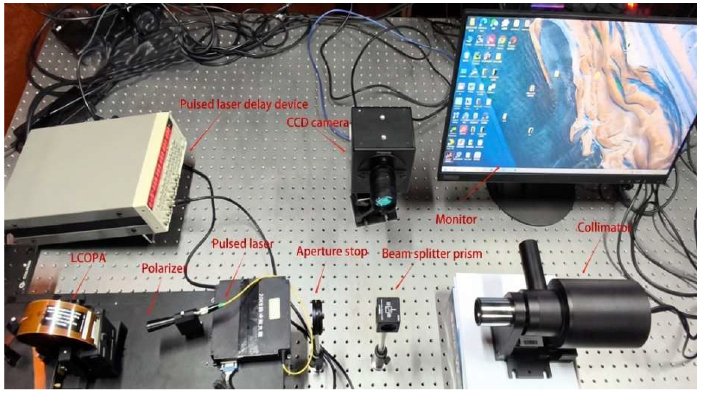
To verify the effectiveness of the modeling method proposed in this paper, a fractional-order modeling experimental platform for the precise beam regulation system of the liquid crystal spatial light modulator shown in Figure 12 is built. The system consists of a pulsed laser, a polarizer, an LCOPA, an aperture, a beam splitter prism, a collimator, a high-speed CCD camera, a delayer and a display. Among them, the wavelength of the incident laser beam is $\lambda =1064 \mathrm{nm}$, the refresh frequency of the driving voltage of the LCOPA is 1000 Hz, and the sampling frequency of the CCD camera is 10 kHz. The main working flow of the system is as follows: the laser first emits 1064 nm laser light; the computer loads stepped grayscale images to the LCOPA to realize controllable beam deflection. Afterwards, the propagation direction of the outgoing beam is adjusted by the beam splitter prism and collimator, and the whole dynamic evolution process of the beam is completely collected by the CCD camera.

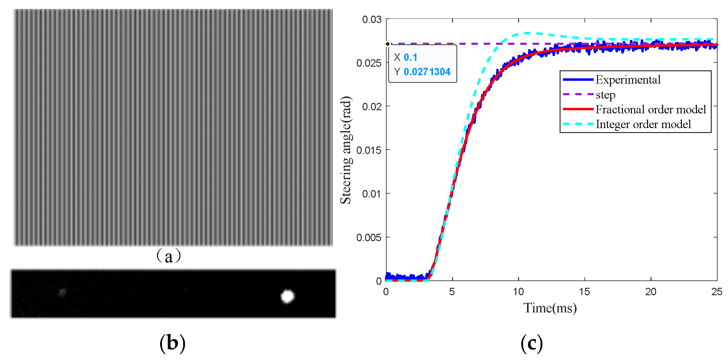
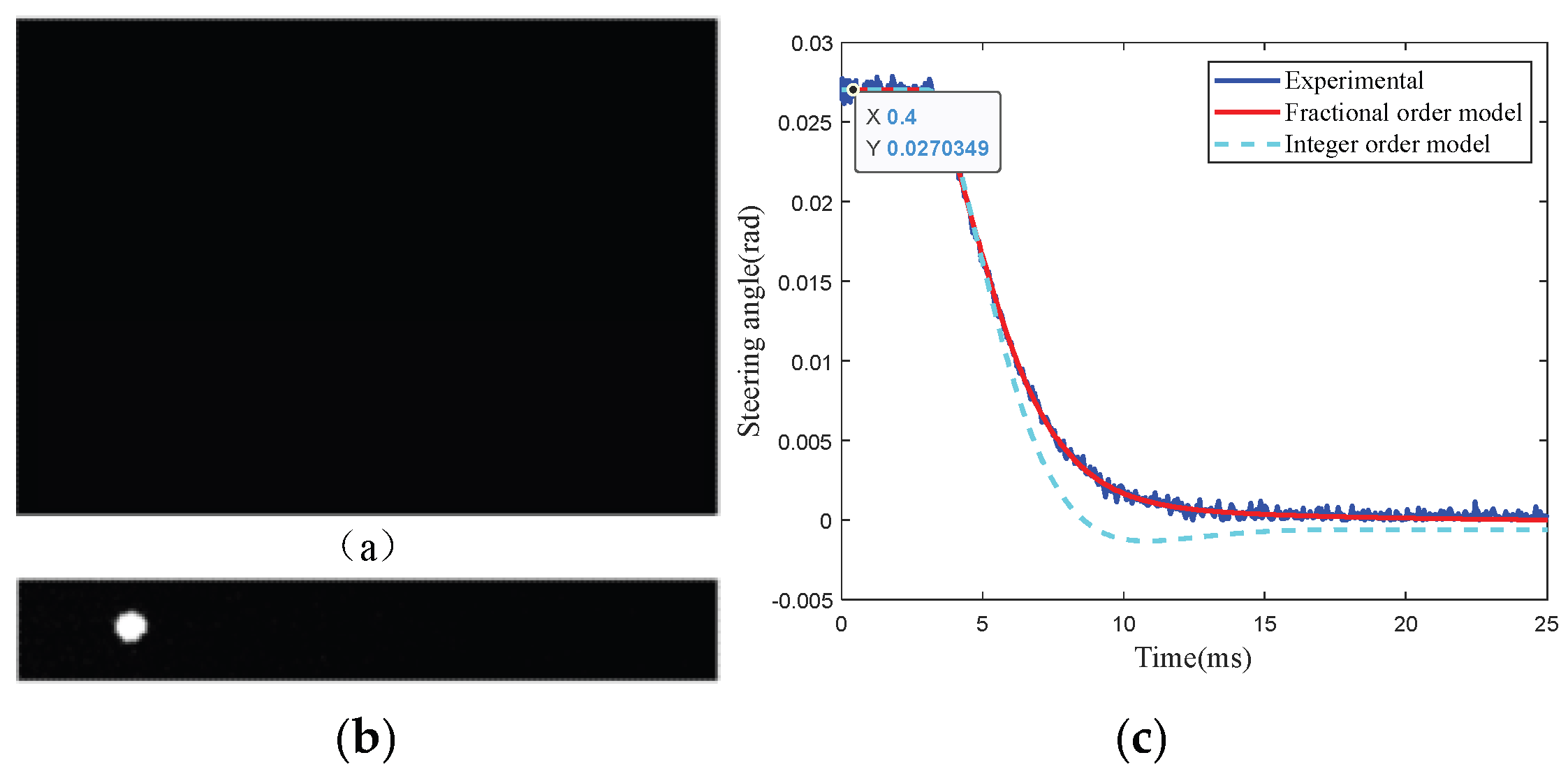
It can be known from the above analysis that the dynamic effects of the x-axis channel and the y-axis channel are the same. Therefore, we select the x-axis channel to verify the dynamic response effect of its model. The grayscale image corresponding to the phase difference $\Delta \phi =\pi /2$ in the azimuth axis direction is loaded into the upper computer, and the beam centroid offset is detected with the help of a CCD camera. The trigonometric function method is used to convert the centroid offset into the actual deflection angle of the beam, and the model parameters are finally identified through the Legendre wavelet integral operational matrix method. Figure 13 and Figure 14 respectively present the fitting comparison results of the fractional-order model and integer-order model for the precise beam regulation system of liquid crystal spatial light modulator.

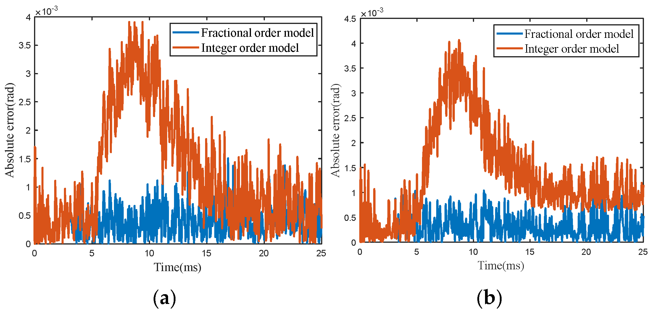
Figure 13 shows that, when a phase difference of $\pi /2$ is applied, the beam deflection angle gradually deflects from 0 rad to 0.0272 rad. The fractional-order model established in this paper can well characterize the dynamic performance of beam deflection, and the key dynamic indicators are shown in

Table 1. Comparison of key dynamic performance indicators between fractional-order and integer-order.

Performance Indicators	Experimental Data	Fractional-Order Model	Integer-Order Model
Rise Time (ms)	4	4	4
Stabilization Time (ms)	10	10	12
Steady-State Value (rad)	0.0272	0.0272	0.0272
Peak Value (rad)	0.0273	0.0273	0.0280
Overshoot	0%	0%	3%

. It can be seen from Figure 14 that, after the voltage is removed, the beam deflection angle gradually deflects from 0.0272 rad to 0 rad, and the fractional-order model can also well simulate the voltage removal process. It can be seen from Figure 15 that the RMSE of the fractional-order model over the entire time interval is 0.00018 rad, with a fitting degree of 98%, while the integer-order model exhibits significant errors in fitting the actual data, verifying the effectiveness of the fractional-order model established in this paper.

In summary, the fractional-order model outperforms the integer-order model in key indicators such as peak value, overshoot, and settling time and can more accurately simulate the dynamic characteristics of the entire cycle of beam deflection.

5.2. Verification of Coupling Effect

To verify the ability of the established fractional-order model to describe the coupling characteristics between channels, this section conducts two sets of experiments, namely single-channel drive and dual-channel drive, to compare and analyze the experimental data with the model simulation results, with a focus on the model’s performance in dynamic tracking error, and to compare the fitting performance of the fractional-order model and the integer-order model. The integer-order model used for horizontal comparison adopts a classical integer-order Kelvin viscoelastic structure whose topology exactly matches that of the fractional-order model in this paper, with all fractional-order differential operators replaced by standard integer-order differential operators while keeping the number and arrangement of elastic and viscous elements unchanged. The two types of models employ a completely unified parameter identification process, share the same set of measured step-response data, and rely on the same viscous wave integral operational matrix algorithm for parameter optimization, with only the differential operator order replaced, and the optimization objective is to minimize the mean square error of the output response to solve for all viscoelastic parameters.

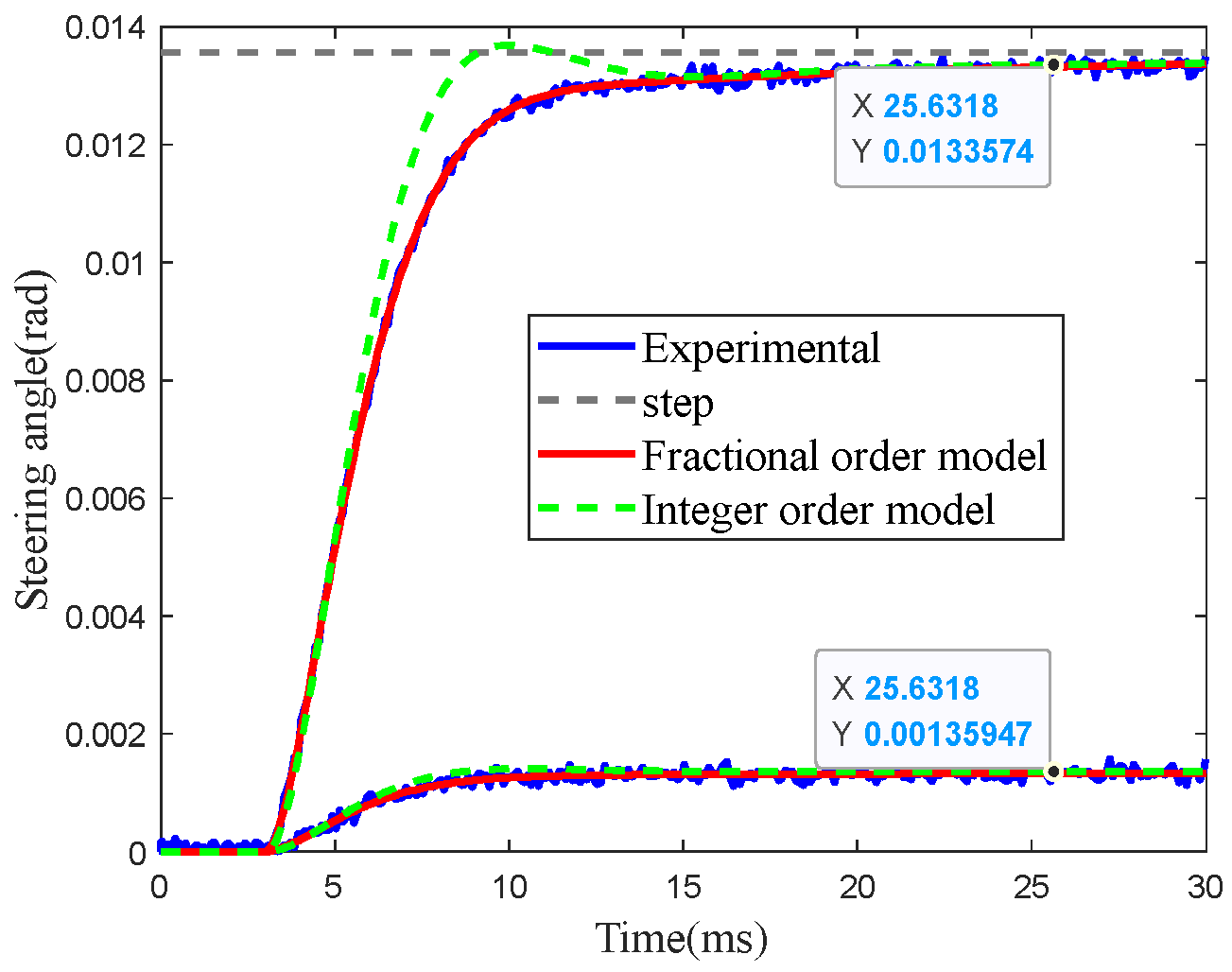
In the single-channel driving experiment, only a step signal with the amplitude of $u_x=\pi /4$ is applied to the $x$-axis (the ideal output is $0.0136 \mathrm{rad}$), and there is no driving input on the $y$-axis. The experimental results are shown in Figure 16.

The experimental results show that, although no driving voltage is applied to the y-axis, a significant coupled deflection is still generated, with a steady-state response amplitude of approximately 8.3% of the main response of the x-axis, which is basically consistent with the cross-coupling gain set in the model. In terms of dynamic tracking performance, the RMSE of the fractional-order model over the entire time interval does not exceed 0.00018 rad, which is significantly lower than that of the integer-order model (RMSE > 0.0011 rad), indicating that the fractional-order model has higher accuracy in characterizing coupled dynamics. In terms of steady-state accuracy, since the steady-state value is determined by the system gain and is independent of the model order selection, both types of models can achieve theoretical steady-state values consistent with the experimental data.

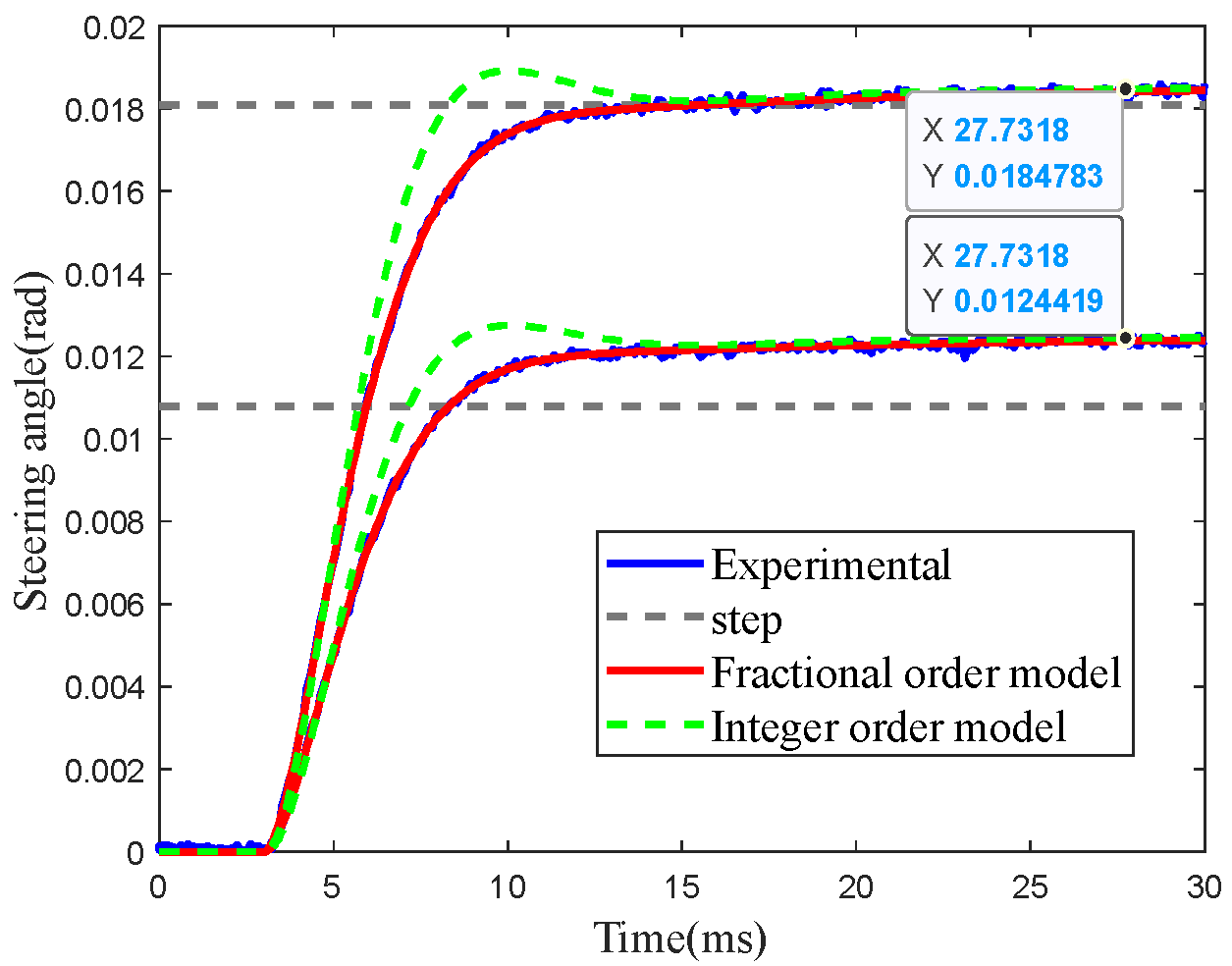
In the dual-channel driving experiment, driving signals of $u_x=\pi /3$ (ideal output of $0.0181 \mathrm{rad}$) and $u_y=\pi /5$ (ideal output of $0.0109 \mathrm{rad}$) are applied to the $x$-axis and $y$-axis, respectively. The experimental results are shown in Figure 17.

The experimental data show that both channels exhibit stable rising and convergence processes, with observable cross-coupling effects between them. Specifically, the actual steady-state response amplitude of the x-axis is approximately 0.0184 rad, and that of the y-axis is approximately 0.0124 rad, both of which are in good agreement with the theoretical set values. In terms of dynamic tracking performance, the RMSE of the fractional-order model over the entire time interval does not exceed 0.00020 rad, which is significantly lower than that of the integer-order model (RMSE > 0.0011 rad), indicating that it also has higher accuracy in characterizing dual-channel coupled dynamics.

Combining the three stages of research in this paper, namely mechanism modeling, parameter identification, and experimental verification, they form a progressively supportive serial relationship: the modeling stage constructs a complete mechanism framework incorporating two-dimensional static propagation, fractional-order viscoelastic constitutive model, channel cross-coupling, and per-channel time delay, establishing the theoretical upper limit of accuracy for high-precision model prediction; the parameter identification stage achieves simultaneous solution of all parameters based on the Legendre wavelet integral operational matrix method, and after identification, the model achieves a fitting degree of 98% for the dynamic process of beam deflection, with a steady-state prediction error of less than 0.15% and a dynamic root mean square error not exceeding 0.00020 rad, and the fitting accuracy at this stage directly determines the final prediction performance of the model; the experimental verification stage, through two sets of comparative tests (single-channel and dual-channel), quantitatively demonstrates that the dynamic performance of the fractional-order coupled model proposed in this paper is significantly superior to that of the traditional integer-order model, intuitively reflecting the performance advantages of the modeling scheme. The three stages form a complete closed-loop logic and jointly determine the quantitative indicators of the final beam steering. For an intuitive summary of the core quantitative indicators mentioned above, including steady-state deflection, rise time, settling time and dynamic RMSE, readers may refer to the table in Section 5.1 and the corresponding numerical results presented in the text of Section 5.2. It should be noted that the dynamic characteristics of both the single-channel data with $u_x=\pi /4$ and the dual-channel data with $u_x=\pi /3$ and $u_y=\pi /5$ used in the above verification are superior to those of the integer-order model, with dynamic root mean square errors in the same order of magnitude, fully demonstrating that the established fractional-order coupled model has good generalization capability.

6. Discussion

This paper addresses the key problems in two-dimensional beam deflection modeling of liquid crystal optical phased arrays, including the difficulty of integer-order models in characterizing viscoelastic memory effects, the difficulty in accurately describing channel cross-coupling, and the complexity of parameter identification for fractional-order models. Following the progressive logic of mechanism modeling, parameter identification, and experimental verification, a systematic study on two-dimensional coupled fractional-order dynamic modeling and parameter identification methods is conducted. By establishing a two-dimensional beam propagation static model based on the radar phased array principle and combining it with the fractional-order generalized Kelvin constitutive equation, a two-dimensional fractional-order dynamic model that simultaneously considers multi-element coupling, channel cross-coupling, and time-delay characteristics is constructed, solving the problem that traditional integer-order models cannot characterize the viscoelastic memory effects of liquid crystals. A parameter identification method based on the Legendre wavelet integral operational matrix is proposed, which transforms fractional-order operations into purely algebraic operations, achieving high-precision simultaneous identification of fractional-order model parameters, with a fitting degree of 98% for the dynamic process. Experimental results show that the steady-state prediction error of the established model is less than 0.15%, and the dual-channel dynamic root mean square errors of the coupled model do not exceed 0.00020 rad, with all indicators significantly superior to those of the integer-order model, providing theoretical support for the design of high-precision beam steering systems. Future research can be further advanced in directions such as fractal–fractional fusion modeling, temperature robustness, fractional-order advanced control algorithms, large-scale array distributed modeling, and machine-learning-assisted identification, promoting the development of liquid crystal optical phased array modeling and control technologies.

References

1. Dashdavaa, E.; Erdenebat, M.-U.; Bayarsaikhan, E.; Seo, J.-H.; Kim, M.-S.; Do, J.; Won, K.; Kim, H.-R. Continuous eyebox expansion in holographic near-eye displays using a liquid crystal tunable active beam deflector. Opt. Lasers Eng. 2026, 196, 109407. [Google Scholar] [CrossRef]
2. Zhao, S.; Chen, J.; Shi, Y. All-Solid-State Beam Steering via Integrated Optical Phased Array Technology. Micromachines 2022, 13, 894. [Google Scholar] [CrossRef] [PubMed]
3. Notaros, M.; DeSantis, D.M.; Raval, M.; Notaros, J. Liquid-crystal-based visible-light integrated optical phased arrays and application to underwater communications. Opt. Lett. 2023, 48, 5269–5272. [Google Scholar] [CrossRef] [PubMed]
4. Zeng, Z.; Li, Z.; Fang, F.; Zhang, X. Phase Compensation of the Non-Uniformity of the Liquid Crystal on Silicon Spatial Light Modulator at Pixel Level. Sensors 2021, 21, 967. [Google Scholar] [CrossRef] [PubMed]
5. Mcmanamon, P.F.; Ataei, A. Progress and opportunities in the development of nonmechanical beam steering for electro-optical systems. Opt. Eng. 2019, 58, 120901. [Google Scholar] [CrossRef]
6. Arias, A.; Paniagua-Diaz, A.M.; Prieto, P.M.; Roca, J.; Artal, P. Phase-only modulation with two vertical aligned liquid crystal devices. Opt. Express 2020, 28, 34180–34189. [Google Scholar] [CrossRef] [PubMed]
7. Yang, Q.; Zou, J.; Li, Y.; Wu, S.-T. Fast-Response Liquid Crystal Phase Modulators with an Excellent Photostability. Crystals 2020, 10, 765. [Google Scholar] [CrossRef]
8. Park, C.; Lee, K.; Baek, Y.; Park, Y. Low-coherence optical diffraction tomography using a ferroelectric liquid crystal spatial light modulator. Opt. Express 2020, 28, 39649–39659. [Google Scholar] [CrossRef] [PubMed]
9. Li, Y.; Yan, J.; Shi, B.; Xuan, W.; Mo, Z.; Wang, H.; Mao, B.; Feng, Z.; Liu, M.; You, Q.; et al. High-precision phase profile modeling for liquid crystal on silicon devices. Appl. Opt. 2025, 64, 10173–10179. [Google Scholar] [CrossRef] [PubMed]
10. Jaggi, C.; Kumar, P. Polyhedral oligomeric silsesquioxane nanoparticles: An effective dopant for homeotropic alignment of liquid crystals with enhanced electro-optic performance. J. Nanopart. Res. 2025, 27, 311. [Google Scholar] [CrossRef]
11. Zou, J.; Yang, Q.; Hsiang, E.-L.; Ooishi, H.; Yang, Z.; Yoshidaya, K.; Wu, S.-T. Fast-Response Liquid Crystal for Spatial Light Modulator and LiDAR Applications. Crystals 2021, 11, 93. [Google Scholar] [CrossRef]
12. Zhou, S.; Cao, J.; Hao, Q.; Li, W.; Sheng, Y.; Chen, H.; Gao, Z.H.; Ji, P. All-solid-state omnidirectional fast scanning using liquid crystal optical phased array and conical mirror. Opt. Express 2025, 33, 18124–18135. [Google Scholar] [CrossRef] [PubMed]
13. Shi, H.; Wei, M.; Liang, F.; Wang, X. Polarization-independent one-dimensional beam-steering liquid-crystal optical phased array using a liquid crystal polarization grating. Opt. Laser Technol. 2026, 199, 114957. [Google Scholar] [CrossRef]
14. Sherpa, N.; Bharadwaj, A.; Kumar, N.; Chauhan, A.; Boruah, B.R. Synchronization and clock recovery in a ferroelectric liquid crystal spatial light modulator based free-space optical communication link. Rev. Sci. Instrum. 2023, 94, 053002. [Google Scholar] [CrossRef] [PubMed]
15. Guo, H.; Wang, X.; Liu, X.; He, X.; Wu, L.; Huang, X.; Xie, X.; Tan, Q.; Cao, J.; Xie, W. Nonmechanical two-user tracking method of space-polarization division using the LCOPA. Opt. Commun. 2019, 447, 74–79. [Google Scholar] [CrossRef]
16. Sager, S.; Gambín, A.; Prieto, P.M.; Artal, P. Binocular adaptive optics visual simulator with convergence control. Biomed. Opt. Express 2025, 16, 4017–4026. [Google Scholar] [CrossRef] [PubMed]
17. Song, M.; Liu, Y.; Lu, F.; Cao, Q.; Zhai, Y. A CNN-GS Hybrid Algorithm for Generating Pump Light Fields in Atomic Magnetometers. Photonics 2025, 12, 796. [Google Scholar] [CrossRef]
18. Sun, D.; Dai, H.; Lin, H.; Qiao, W.; Zhang, Z.; Li, S.; Ruan, J. Beam Shaping of VCSEL Arrays Utilizing Liquid Crystal Spatial Light Modulation. IEEE Photonics Technol. Lett. 2025, 37, 1097–1100. [Google Scholar] [CrossRef]
19. Cai, W.; Chen, W.; Xu, W. Characterizing the creep of viscoelastic materials by fractal derivative models. Int. J. Non-Linear Mech. 2016, 87, 58–63. [Google Scholar] [CrossRef]
20. Kothari, K.; Mehta, U.; Vanualailai, J. A novel approach of fractional-order time delay system modeling based on Haar wavelet. ISA Trans. 2018, 80, 371–380. [Google Scholar] [CrossRef] [PubMed]
21. Zhang, W.; Pivnenko, M.; Chu, D. High-efficiency phase modulation in LCoS-compatible LC-metasurface via spacer integration and Oseen-Frank modeling. Opt. Express 2025, 33, 46187–46198. [Google Scholar] [CrossRef] [PubMed]
22. Qi, M.; Wang, Q.; Mu, Q.; Liu, Y.; Yao, L.; Cao, Z.; Zhang, H.; Yang, C.; Hu, L.; Xuan, L. Study of Response Time Depending on Driving Voltage of Liquid Crystal Spatial Light Modulator. Laser Optoelectron. Prog. 2013, 50, 092302. [Google Scholar] [CrossRef]
23. Zhang, B. Dynamic Response and Hysteresis Simulation Calculation of Blue Phase Liquid Crystal Displays. Master’s Thesis, Hebei University of Technology, Tianjin, China, 2023. [Google Scholar]
24. Li, Y.; Yang, Z.; Chen, R.; Mo, L.; Li, J.; Hu, M.; Wu, S.-T. Submillisecond-Response Polymer Network Liquid Crystal Phase Modulators. Polymers 2020, 12, 2862. [Google Scholar] [CrossRef] [PubMed]
25. Márquez, A.; Martínez-Guardiola, F.J.; Francés, J.; Neipp, C.; Ramírez, M.G.; Calzado, E.M.; Morales-Vidal, M.; Gallego, S.; Beléndez, A.; Pascual, I. Analytical modeling of blazed gratings on two-dimensional pixelated liquid crystal on silicon devices. Opt. Eng. 2020, 59, 041208. [Google Scholar] [CrossRef]
26. Lin, Y.; Ai, Y.; Shan, X.; Liu, M. Liquid crystal based non-mechanical beam tracking technology. Opt. Laser Technol. 2017, 91, 103–107. [Google Scholar] [CrossRef]
27. Wang, C.Y.; Li, L.T.; Shi, H.W.; Niu, Q.F. Research on Beam Deflection Control Method Based on Liquid Crystal Phased Array. Chin. J. Liq. Cryst. Disp. 2018, 33, 58–65. [Google Scholar] [CrossRef]
28. Wang, Z.; Wang, C.; Liang, S.; Liu, X. Liquid crystal spatial light modulator based non-mechanical beam steering system fractional-order model. Opt. Express 2022, 30, 12178. [Google Scholar] [CrossRef] [PubMed]
29. Zhang, Y.; Wang, Q.; Jiang, H.; Peng, Z.; Mu, Q.; Wang, C.; Wang, Y. Dynamic response characteristics of optical beam deflection in LCOPA. Opt. Express 2024, 32, 35733. [Google Scholar] [CrossRef] [PubMed]
30. Lesina, A.C.; Goodwill, D.; Bernier, E.; Ramunno, L.; Berini, P. On the performance of optical phased array technology for beam steering: Effect of pixel limitations. Opt. Express 2020, 28, 31637–31657. [Google Scholar] [CrossRef]
31. Tang, Y.; Li, N.; Liu, M.; Lu, Y.; Wang, W. Identification of fractional-order systems with time delays using block pulse functions. Mech. Syst. Signal Process. 2017, 91, 382–394. [Google Scholar] [CrossRef]
32. Pawale, T.; Swain, J.; Hashemi, M.R.; Tierra, G.; Li, X. Dynamic Motions of Topological Defects in Nematic Liquid Crystals under Spatial Confinement. Adv. Mater. Interfaces 2023, 10, 2300136. [Google Scholar] [CrossRef]
33. Wang, Z.; Wang, C.; Ding, L.; Wang, Z.; Liang, S. Parameter identification of fractional-order time delay system based on Legendre wavelet. Mech. Syst. Signal Process. 2022, 163, 108141. [Google Scholar] [CrossRef]
34. Khellat, F.; Yousefi, S.A. The linear Legendre mother wavelet operational matrix of integration and its application. J. Frankl. Inst. 2006, 343, 181–190. [Google Scholar] [CrossRef]
35. Tang, Y.; Liu, H.; Wang, W.; Lian, Q.; Guan, X. Parameter identification of fractional order systems using block pulse functions. Signal Process. 2015, 107, 272–281. [Google Scholar] [CrossRef]
36. Wu, J.-L.; Chen, C.-H.; Chen, C.-F. Numerical inversion of Laplace transform using Haar wavelet operational matrices. IEEE Trans. Circuits Syst. I-Regul. Pap. 2001, 48, 120–122. [Google Scholar] [CrossRef]
37. Giusti, A.; Colombaro, I.; Garra, R.; Garrappa, R.; Mentrelli, A. On variable-order fractional linear viscoelasticity. Fract. Calc. Appl. Anal. 2024, 27, 1564–1578. [Google Scholar] [CrossRef]
Figure 1. N-dimensional uniform LCOPA.
Fractalfract 10 00499 g001
Figure 2. Model of the n-th radiation source.
Fractalfract 10 00499 g002
Figure 3. Far-field light intensity distributions of one-dimensional LCOPA at different angles.
Fractalfract 10 00499 g003
Figure 4. Geometric schematic diagram of two-dimensional LCOPA.
Fractalfract 10 00499 g004
Figure 5. Far-field light intensity distribution of two-dimensional beam. (a) Far-field distribution diagram of original light spot; (b) far-field distribution diagram with light spot deflected to (20°, 10°).
Fractalfract 10 00499 g005
Figure 6. Structural diagram of LCOPA. (a) Without applied voltage; (b) with applied voltage.
Fractalfract 10 00499 g006
Figure 7. Fractional-order Kelvin viscoelastic model.
Fractalfract 10 00499 g007
Figure 8. Fractional-order Kelvin viscoelastic model of LCOPA under multi-element coupling.
Fractalfract 10 00499 g008
Figure 9. Schematic diagram of liquid crystal molecular director.
Fractalfract 10 00499 g009
Figure 10. Spatial distribution of molecular directors in LCOPA.
Fractalfract 10 00499 g010
Figure 11. Averaged liquid crystal molecular tilt angle and fitting curve.
Fractalfract 10 00499 g011
Figure 12. Two-dimensional beam deflection data acquisition platform.
Fractalfract 10 00499 g012
Figure 13. Comparison results between the integer-order model and fractional-order model when loading the grayscale image with Δ φ = π / 2 . (a) Grayscale pattern loaded; (b) beam steering result; (c) model comparison result.
Fractalfract 10 00499 g013
Figure 14. Comparison results between the integer-order model and fractional-order model when removing the grayscale image with Δ φ = π / 2 . (a) Grayscale pattern loaded; (b) beam steering result; (c) model comparison result.
Fractalfract 10 00499 g014
Figure 15. Point-by-point error curves during power-on and power-off when loading the grayscale image with Δ φ = π / 2 . (a) Loading the grayscale image; (b) removing the grayscale image.
Fractalfract 10 00499 g015
Figure 16. Two-axis dynamic response when driving is only applied to the x -axis.
Fractalfract 10 00499 g016
Figure 17. Two-axis dynamic response under simultaneous dual-channel driving.
Fractalfract 10 00499 g017