Fractional Retarded Dynamic Equations on Time Scales with Δ-HKP Integral

Abstract

This paper investigates the existence of pseudosolutions for a class of fractional retarded dynamic equations on time scales in Banach spaces endowed with the weak topology. The proposed model combines fractional dynamics, explicit delay effects, and hybrid continuous–discrete temporal structures within a unified analytical framework. The analysis is performed by means of the $\Delta$-Henstock–Kurzweil–Pettis integral, allowing significantly weaker regularity assumptions than those required by classical integration theories. The existence result is established using the De Blasi measure of weak noncompactness together with Kubiaczyk’s fixed point theorem for weakly sequentially continuous operators. The obtained theorem extends several existing results on fractional differential equations and dynamic equations on time scales by incorporating explicit delays and generalized integration into a common framework. The obtained results provide a unified analytical framework for studying hereditary systems evolving on hybrid time domains.

1. Introduction

Differential equations constitute one of the principal mathematical tools for describing dynamic phenomena arising in natural sciences, engineering, economics, and many interdisciplinary areas. In numerous realistic models, however, the evolution of a system depends not only on its current state but also on its past history. Such memory effects naturally occur in population dynamics, where the growth rate depends on maturation time, in epidemiology through incubation periods, in economics where investment decisions and business cycles are influenced by previous values of macroeconomic indicators, and in control theory where delayed feedback plays a fundamental role in the system dynamics. These observations have led to the extensive development of the theory of retarded differential equations, which provides an appropriate mathematical framework for modeling hereditary systems and processes with aftereffects.

During the recent decades, fractional calculus has become an increasingly important tool for modeling phenomena involving memory and hereditary properties. In contrast to classical integer-order derivatives, fractional derivatives incorporate information from the entire history of a process and therefore provide a more realistic description of many physical and engineering systems. Applications of fractional differential equations include anomalous diffusion, viscoelastic materials, thermal processes, electrical circuits, biological systems, and financial mathematics [1,2,3,4,5]. Owing to their nonlocal character, fractional models have proved to be more accurate than classical models in describing complex dynamical behavior.

Recent years have also witnessed successful applications of fractional-order models in epidemiology, particularly in the analysis of COVID-19 dynamics involving quarantine, vaccination, and environmental viral load [6,7,8]. Their ability to incorporate memory effects has significantly improved model realism and prediction accuracy.

Another important direction of research is provided by the theory of time scales, which unifies differential and difference equations within a common mathematical framework. Its general foundations and the theory of dynamic equations are developed in [9,10,11,12]. Specific advances include inequalities on time scales [13], economic applications [14,15], and integration theory on time scales [16,17]. Quantum and q-calculus, which are closely connected with discrete and quantum time scales, are presented in [18]. Weak existence results for dynamic Cauchy problems are obtained in [19], whereas Fredholm-type integro-differential equations on time scales are studied in [20]. As a consequence, fractional calculus on time scales has emerged as a natural extension of classical fractional analysis, allowing memory effects to be studied on continuous, discrete, quantum, and hybrid temporal domains.

In many practical applications, however, memory effects arise from two independent mechanisms. The first one is represented by the fractional derivative, reflecting the hereditary nature of the process, whereas the second originates from explicit delays describing the dependence of the present state on past values of the unknown function. Such phenomena occur in neural networks with transmission delays, physiological control systems, epidemiological models involving incubation periods, ecological systems with maturation delays, and engineering systems with delayed feedback. Consequently, fractional retarded dynamic equations on time scales provide a natural mathematical model for systems possessing hereditary properties, explicit delays, and hybrid continuous–discrete temporal evolution simultaneously.

Recent advances in control theory have led to the development of stochastic, cyber-physical, intelligent, and networked control systems [21,22]. Fractional-order control strategies for networked systems with delays and fault-tolerant intelligent control have recently been investigated in [23,24]. Fractional-order models play an important role in these areas owing to their ability to describe hereditary effects and delayed dynamics. Consequently, rigorous existence results provide an essential analytical foundation for subsequent studies on controllability, stabilization, and optimal control.

From the analytical viewpoint, many nonlinear operators satisfy only weak sequential continuity assumptions and lack the compactness required by classical fixed point methods. This motivates the use of the $\Delta$-Henstock–Kurzweil–Pettis integral together with weak topological techniques for proving existence results under weaker regularity assumptions [17,25].

In recent years, fractional delay differential equations have attracted considerable attention. Existence and stability results for fractional delay differential equations are established in [26,27]. Hyers–Ulam-type stability for Caputo fractional delay systems is investigated in [28,29]. Uniqueness and generalized Ulam stability for delayed multi-term fractional equations are studied in [30,31]. A linearized stability theorem for nonlinear delay fractional differential equations is established in [32]. Recent studies have demonstrated a growing interest in fractional dynamic equations on time scales, including existence, stability, and qualitative properties of solutions under various assumptions [33,34]. Furthermore, abstract dynamic equations in Banach spaces and generalized integro-dynamic models on time scales have recently been investigated using fixed point techniques and measures of noncompactness [35,36].

Nevertheless, the simultaneous incorporation of explicit delays, Caputo fractional dynamics, the $\Delta$-Henstock–Kurzweil–Pettis integral, and weak topological methods has not yet been addressed. In particular, the theory of fractional retarded dynamic equations on time scales involving the $\Delta$-HKP integral and formulated in Banach spaces endowed with the weak topology remains essentially undeveloped.

Retarded fractional dynamic equations naturally arise in delayed feedback, adaptive, sampled-data, and distributed parameter systems. The existence theorem established in this paper guarantees the existence of admissible trajectories and provides a mathematical foundation for subsequent studies on controllability, stabilization, and optimal control.

In this paper, we study a class of fractional retarded dynamic equations on time scales in a Banach space E of the form

$${}_T{}^C\Delta ^{\alpha }x\left(t\right)=f(t,x_t),$$

(1)

with the initial condition

$$x\left(\theta \right)=\phi \left(\theta \right),\theta \in I_r=[-r,0]\cap \mathbb{T},$$

where $x_t\left(\theta \right)=x(t+\theta )$, $r>0$ is a fixed real number, $\phi$ is a given function, and $\mathbb{T}$ denotes a time scale. Moreover, we assume that $f:I_a\times C(I_r,E)\to E$ is $\Delta$-HKP-integrable.

Since translations on general time scales are not always generated by additive shifts, the notation $x_t$ should be understood as the history segment obtained whenever $t+\theta \in \mathbb{T}$. Throughout this paper, we assume that the chosen interval guarantees the existence of these translated arguments.

These equations incorporate memory effects resulting from both the delay and the fractional order of the derivative, as well as a hybrid time structure. The analysis is carried out in the weak topology using the De Blasi measure of weak noncompactness and fixed point methods for weakly sequentially continuous mappings.

The main objective of this paper is to establish sufficient conditions for the existence of pseudosolutions to the considered problem. The obtained results extend existing contributions and contribute to the development of the modern theory of dynamic equations, providing tools for the analysis of complex systems with memory, delay, and continuous–discrete structure.

To better emphasize the novelty of the proposed approach, we briefly compare it with the most closely related contributions available in the literature. Salem et al. [37] investigated fractional differential equations in Banach spaces but did not consider delay effects, time scales, or generalized integration techniques. Kubiaczyk and Sikorska-Nowak [19] established a weak topological framework for dynamic equations on time scales; however, their analysis was restricted to classical dynamic equations and did not involve fractional operators. Sikorska-Nowak [34] extended this line of research by introducing the $\Delta$-Henstock–Kurzweil–Pettis integral into fractional dynamic equations on time scales, although explicit delays were not included. More recently, Nisar et al. [33] investigated fractional dynamic equations on time scales using classical fixed point techniques, but without employing the $\Delta$-HKP integral or weak topological methods. To the best of the authors’ knowledge, the present paper is the first to combine explicit delay, fractional dynamics, arbitrary time scales, the $\Delta$-Henstock–Kurzweil–Pettis integral, weak sequential continuity, the De Blasi measure of weak noncompactness, and Kubiaczyk’s fixed point theorem within a unified existence framework. Consequently, the obtained existence theorem unifies several previously independent research directions and substantially extends the available existence theory for hereditary dynamical systems evolving on arbitrary time scales.

2. Preliminaries

Let $(E,\parallel ·\parallel )$ be a Banach space and let $E^{\ast }$ be its dual space. Denote, by $(C(I_a,E),\omega )$, the space of all continuous functions from $I_a$ to E endowed with the topology

$$\sigma \left(C(I_a,E),C{(I_a,E)}^{\ast }\right),$$

and, by $C_{rd}(I_a,E)$, denote the space of all rd-continuous functions from the time scale interval $I_a$ to E. By ${\mu }_{\Delta }$, we denote the Lebesgue measure on the time scale $\mathbb{T}$. For a precise definition and basic properties of this measure, we refer the reader to [16].

This section summarizes the notation and auxiliary concepts required in the subsequent analysis. For completeness, we briefly recall several standard notions from the theory of time scales and generalized integration that will be used throughout the paper. Detailed expositions of these topics can be found in the literature cited below, and only the concepts directly needed in the proof of the main theorem are presented here.

2.1. Time Scale Calculus

For the convenience of the reader and to facilitate the exposition, we introduce some preliminary definitions and notations related to time scales, commonly found in the literature (see references [10,11,38,39,40] and the cited papers therein).

A time scale $\mathbb{T}$ is a nonempty closed subset of real numbers $\mathbb{R}$, with the subspace topology inherited from the standard topology of $\mathbb{R}$.

By an interval $I_a$, we mean the time scale interval

$$I_a=[0,a]\cap \mathbb{T}=\{t\in \mathbb{T}:0\le t\le a\}={[0,a]}_{\mathbb{T}}.$$

Throughout this paper, all intervals are understood as intervals on a time scale.

Definition 1. 

The forward jump operator $\sigma :\mathbb{T}\to \mathbb{T}$ and the backward jump operator $\rho :\mathbb{T}\to \mathbb{T}$ are defined as $\sigma \left(t\right)=inf\{s\in \mathbb{T}:s>t\}$ and $\rho \left(t\right)=sup\{s\in \mathbb{T}:s<t\}$, respectively. We put $infØ=inf\mathbb{T}$ (i.e., $\rho \left(m\right)=m$ if $\mathbb{T}$ has a minimum m).

The jump operators $\sigma$ and $\rho$ allow the classification of points in time scale in the following way: t is called right-dense, right-scattered, left-dense, left-scattered, dense and isolated if $\sigma \left(t\right)=t,\sigma \left(t\right)>t,\rho \left(t\right)=t,\rho \left(t\right)<t,\rho \left(t\right)=t=\sigma \left(t\right),\rho \left(t\right)<t<\sigma \left(t\right),$ respectively.

Definition 2. 

We say that a function k is right-dense continuous (rd-continuous) if k is continuous at every right-dense point $t\in \mathbb{T}$ and

$$\underset{s\to t^{-}}{lim}k\left(s\right)$$

exists and is finite at every left-dense point $t\in \mathbb{T}$.

The fundamental differential operator on a time scale is the $\Delta$-derivative, recalled below for completeness.

Definition 3. 

Fix $t\in \mathbb{T}$. Let $f:I_a\to E$. Then, we define Δ-derivative of f by

$$f^{\Delta }\left(t\right)=\underset{s\to t}{lim}{\displaystyle \frac{f\left(\sigma \right(t\left)\right)-f\left(s\right)}{\sigma \left(t\right)-s}}.$$

The function f is called Δ-differentiable on $\mathbb{T}$, if for each $t\in \mathbb{T}$ there exists $f^{\Delta }\left(t\right)$.

Note that

(1)

$f^{\Delta }=f^{\prime }$ is the usual derivative if $\mathbb{T}=\mathbb{R}$;

(2)

$f^{\Delta }=\Delta f$ is the usual forward difference operator if $\mathbb{T}=\mathbb{Z}$;

(3)

$f^{\Delta }=D_{q}f={\displaystyle \frac{f\left(qt\right)-f\left(t\right)}{(q-1)t}}$ is the q-derivative or the delta derivative on the q-time scale if $\mathbb{T}=q^{{\mathbb{N}}_0}=\{q^t:t\in {\mathbb{N}}_0,q>1\}$.

Therefore, the delta derivative provides a common framework encompassing classical differentiation, forward difference operators, and $q-$calculus as particular cases. This unifying property constitutes one of the principal advantages of the time-scale approach (see [10,11], for instance).

2.2. The $\Delta$-Henstock-Kurzweil-Pettis Integral and Fractional Operators

Since the existence theory developed in this paper relies on generalized integration, we next recall the vector-valued $\Delta$-Henstock–Kurzweil integral together with the corresponding Pettis extension.

We will use the notation

$$\eta \left(t\right):=\sigma \left(t\right)-t$$

where $\eta$ is called the graininess function and

$$\nu \left(t\right):=t-\rho \left(t\right),$$

where $\nu$ is called the left-graininess function.

We say that $\delta =({\delta }_L,{\delta }_R)$ is a $\Delta$-gauge for time scale interval $[a,b]$ provided

$${\delta }_L\left(t\right)>0\mathrm{on}(a,b],$$

$${\delta }_R\left(t\right)>0\mathrm{on}[a,b),$$

$${\delta }_L\left(t\right)\ge 0,{\delta }_R\left(t\right)\ge 0$$

and

$${\delta }_R\left(t\right)\ge \eta \left(t\right)$$

for all $t\in [a,b)$.

We say that a partition D for a time scale interval $[a,b]$ given by

$$D=\{a=t_0\le {\xi }_1\le t_1\le \cdots \le t_{n-1}\le {\xi }_n\le t_n=b\}$$

with $t_i>t_{i-1}$, for $1\le i\le n$ and $t_i,{\xi }_i\in \mathbb{T}$ is $\delta$-fine if

$${\xi }_i-{\delta }_L\left({\xi }_i\right)\le t_{i-1}<t_i\le {\xi }_i+{\delta }_R\left({\xi }_i\right),$$

for $1\le i\le n$.

Definition 4. 

A function

$$f:{[a,b]}_{\mathbb{T}}\to E$$

is the Henstock–Kurzweil Δ-integrable on ${[a,b]}_{\mathbb{T}}$ (Δ-HK-integrable in short) if there exists a function

$$F:{[a,b]}_{\mathbb{T}}\to E,$$

defined on the subintervals of ${[a,b]}_{\mathbb{T}}$, satisfying the following property: given $\epsilon >0$, there exists a positive function δ on ${[a,b]}_{\mathbb{T}}$ such that $D=\{{[u,v]}_{\mathbb{T}},\xi \}$ is the δ-fine division of a ${[a,b]}_{\mathbb{T}}$. Thus, we have

$$∥\sum _D\left(f\left(\xi \right)(v-u)-\left(F\right(v)-F(u\left)\right)\right)∥<\epsilon .$$

Definition 5. 

The function $f:I_a\to E$ is Δ–Henstock–Kurzweil–Pettis-integrable (Δ–HKP-integrable for short) if

(1.) 

$\forall x^{\ast }\in E^{\ast },x^{\ast }f$ is Henstock–Kurzweil Δ–integrable on $I_a$.

(2.) 

$\forall t\in I_a\forall x^{\ast }\in E^{\ast },x^{\ast }g\left(t\right)=(\Delta \mathit{-HK}){\int }_0^t{x}^{\ast }f\left(s\right)\Delta s.$

The function g will be called a primitive of f and by $g\left(t\right)=(\Delta \mathit{-HKP}){\int }_0^{t}f\left(s\right)\Delta s$ we will denote the Δ-Henstock–Kurzweil–Pettis integral of f on the interval $I_a$.

Examples illustrating the difference between the $\Delta$-HKP integral and the classical Pettis and $\Delta$-Henstock–Kurzweil integrals are presented in [17].

Theorem 1. 

Suppose that $f,f_n:[a,b]\to E,n=1,2,\dots$, are Δ-HKP-integrable functions. Let $F_n$ be a primitive of $f_n$. If one assumes the following, then f is Δ-HKP-integrable on $I_a$ and ${\int }_0^t{f}_n\left(s\right)\Delta s$ tends weakly in E to ${\int }_0^{t}f\left(s\right)\Delta s$ for each $t\in I_a$.

(1.) 

$\forall x^{\ast }\in E^{\ast },x^{\ast }{f}_n\left(x\right)\to x^{\ast }f\left(x\right){\mu }_{\Delta }\mathit{-almost}\mathit{everywhere}\mathit{on}{I}_a$.

(2.) 

$\forall x^{\ast }\in E^{\ast }$ the family $G=\{x^{\ast }{F}_n:n=1,2,\dots \}$ is uniformly $AC{G}^{\ast }$ on $I_a$ (i.e., weakly uniformly $AC{G}^{\ast }$ on $I_a$).

(3.) 

$\forall x^{\ast }\in E^{\ast }$ the set G is equicontinuous on $I_a$.

Theorem 2. 

[Mean Value Theorem] For each Δ-subinterval $[c,d]\subset [a,b]$, if the integral

$$(\Delta \mathit{-HKP}){\int }_c^{d}y\left(s\right)\Delta s$$

exists, then we have

$$(\Delta \mathit{-HKP}){\int }_c^{d}y\left(s\right)\Delta s\in {\mu }_{\Delta }\left([c,d]\right)·\overline{conv}y\left([c,d]\right),$$

where

$$\overline{conv}y\left([c,d]\right)$$

denotes the close convex hull of the set $y\left(\right[c,d\left]\right)$.

We conclude the preliminary material by recalling the notions of fractional integration and the Caputo fractional derivative on arbitrary time scales.

Definition 6. 

Suppose that $\mathbb{T}$ is a time scale. The Caputo fractional derivative of g is defined by

$${}_{\mathbb{T}}{}^C\Delta ^{\alpha }g\left(t\right)={\displaystyle \frac{1}{\mathrm{\Gamma }(n-\alpha )}}{\int }_0^t{(t-s)}^{n-\alpha -1}{g}^{{\Delta }^n}\left(s\right)\Delta s,t\in I_a,$$

where $n=\left[\alpha \right]+1$ and $\left[\alpha \right]$ denotes the integer part of α and integral is taken in the sense of Δ-HKP, Γ is the Gamma function.

Definition 7. 

Suppose that $\mathbb{T}$ is a time scale, $g:I\to E$ is Δ-HKP-integrable function. The fractional Δ-HKP integral of the order $\alpha \in {\mathbb{R}}^{+}$ of g is defined by

$$I^{\alpha }g\left(t\right)={\int }_a^t{\displaystyle \frac{{(t-s)}^{\alpha -1}}{\mathrm{\Gamma }\left(\alpha \right)}}g\left(s\right)\Delta s,$$

where integral is taken in the sense of Δ-HKP and Γ is the Gamma function.

Remark 1. 

It should be emphasized that the fractional kernel ${(t-s)}^{\alpha -1}$ is always interpreted together with the corresponding Δ-integral on the underlying time scale. Thus, the integration is performed exclusively over admissible points of $\mathbb{T}$. In particular, for $\mathbb{T}=R$, the operator coincides with the classical Caputo fractional integral. For $\mathbb{T}=Z$, the Δ-integral reduces to a discrete delta sum, yielding the corresponding discrete fractional convolution. Therefore, the same analytical formulation consistently covers continuous, discrete, quantum, and hybrid time scales.

2.3. Weak Topological Tools

The principal compactness-type tool employed in the sequel is the De Blasi measure of weak noncompactness, whose basic properties are recalled below.

The deBlasi measure of weak noncompactness $\beta \left(A\right)$ is defined by

$$\beta \left(A\right)=inf\{t>0:\mathrm{there}\mathrm{exists}C\in K^{\omega }\mathrm{such}\mathrm{that}A\subset C+t{B}_0\},$$

where $K^{\omega }$ is the set of weakly compact subsets of E and $B_0$ is the norm unit ball in E.

The properties of the measure of noncompactness $\beta \left(A\right)$ are as follows:

(i)

If $A\subset B$, then $\beta \left(A\right)\le \beta \left(B\right)$;

(ii)

$\beta \left(A\right)=0$ if and only if A is relatively weakly compact;

(iii)

$\beta (A\cup B)=max\left\{\beta \right(A),\beta (B\left)\right\}$;

(iv)

$\beta \left({\overline{A}}^{\omega }\right)=\beta \left(A\right)$, where ${\overline{A}}^{\omega }$ denotes the weak closure of A;

(v)

$\beta \left(\lambda A\right)=\left|\lambda \right|\beta \left(A\right)$, $(\lambda \in \mathbb{R})$;

(vi)

$\beta (A+B)\le \beta \left(A\right)+\beta \left(B\right)$;

(vii)

$\beta (conv(A\left)\right)=\beta \left(A\right)$, where $conv\left(A\right)$ denotes the convex extension of A.

Theorem 3. 

[19] Let $H\subset C(I_a,E)$ be a family of strongly equicontinuous functions. Let $H\left(t\right)=\left\{h\right(t)\in E:h\in H\},$ for $t\in I_a$ and $H\left(I_a\right)={\bigcup }_{t\in I_a}H\left(t\right)$. Then,

$${\beta }_C\left(H\right)=\underset{t\in I_a}{sup}\beta \left(H\left(t\right)\right)=\beta \left(H\left(I_a\right)\right),$$

where ${\beta }_C\left(H\right)$ denotes the measure of noncompactness in $C(I_a,E)$, and the function $t\mapsto \beta \left(H\right(t\left)\right)$ is continuous.

Definition 8. 

A function $f:I_a\to E$ is said to be weakly continuous if it is continuous from $I_a$ to E endowed with its weak topology. A function $g:E\to E_1$, where E and $E_1$ are Banach spaces, is said to be weakly sequentially continuous if for each weakly convergent sequence $\left(x_n\right)$ in E, the sequence $\left(g\left(x_n\right)\right)$ is weakly convergent in $E_1$.

When the sequence $x_n$ tends weakly to $x_0$ in E, we will write $x_n\stackrel{\omega }{\to }{x}_0$.

Definition 9 

([40]). A family $\mathcal{F}$ of functions F is said to be uniformly absolutely continuous in the restricted sense on A or, in short, uniformly $A{C}_{\ast }\left(A\right)$ if for every $\epsilon >0$ there is $\eta >0$, such that for every F in $\mathcal{F}$ and for every finite or infinite sequence of non-overlapping intervals $\left\{[a_i,b_i]\right\}$ with $a_i,b_i\in A$, and satisfying ${\sum }_i|b_i-a_i|<\eta ,$ we have ${\sum }_i\omega (F,[a_i,b_i])<\epsilon ,$ where ω denotes the oscillation of F over $[a_i,b_i]$.

A family $\mathcal{F}$ of functions F is said to be uniformly generalized absolutely continuous in the restricted sense on $[a,b]$ or uniformly $AC{G}_{\ast }\left([a,b]\right)$ if $[a,b]$ is the union of a sequence of closed sets $A_i$ such that on each $A_i$ the function F is uniformly $A{C}_{\ast }\left(A_i\right)$.

The existence result established in Section 3 is based on the following fixed point theorem according to Kubiaczyk.

Theorem 4 

([41]). Let X be a metrizable locally convex topological vector space. Let D be a closed convex subset of X, and let F be a weakly-weakly sequentially continuous map from D into itself. If for some $x\in D$, the implication that

$$\overline{V}=\overline{conv}(\left\{x\right\}\cup F\left(V\right))⟹V\mathit{is}\mathit{relatively}\mathit{weakly}\mathit{compact}$$

(2)

holds for every subset V of D, then F has a fixed point.

3. Main Problem

Let $r,a$ be non-negative real numbers, $I_a={[0,a]}_{\mathbb{T}}$, $a>0$. Let x be some function defined on ${[-r,a]}_{\mathbb{T}}$. For any $t\in I_a$, the function $x_t$ is defined as $x_t\left(\theta \right)=x(\theta +t),$ where $\theta \in I_r={[-r,0]}_{\mathbb{T}}.$ Here, $\theta$ may be a function involving t.

Let $f:I_a\times C(I_r,E)\to E$ and

$${}_{\mathbb{T}}{}^C\Delta ^{\alpha }x\left(t\right)=f(t,x_t),$$

$$x\left(\theta \right)=\phi \left(\theta \right),$$

where $\alpha \in (0,1]$ and $\phi$ is some specified function.

We will consider the following problem:

$$x\left(t\right)=\phi \left(\theta \right)+{\displaystyle \frac{1}{\mathrm{\Gamma }\left(\alpha \right)}}{\int }_0^t{(t-s)}^{\alpha -1}f(s,x_s)\Delta s,t\in I_a,$$

(3)

where the integral is taken in the sense of fractional $\Delta$-HKP integrals.

Fix $x^{\ast }\in E^{\ast }$ and consider the following problem:

$${}_{\mathbb{T}}{}^C\Delta ^{\alpha }\left(x^{\ast }x\right)\left(t\right)=x^{\ast }\left(f(t,x_t)\right),x\left(\theta \right)=\phi \left(\theta \right),t\in I_a.$$

Let us introduce a definition.

Definition 10. 

Let $F:I\to E$ and let $A\subset I$. The function $f:A\to E$ is a fractional pseudo Δ-derivative of F on A if, for each $x^{\ast }\in E^{\ast }$, the real-valued function $x^{\ast }F$ is ${}_{\mathbb{T}}{}^C\Delta ^{\alpha }$-differentiable ${\mu }_{\Delta }$ almost everywhere on A and ${}_{\mathbb{T}}{}^C\Delta ^{\alpha }\left(x^{\ast }F\right)=x^{\ast }f{\mu }_{\Delta }\mathit{-almost}\mathit{everywhere}\mathit{on}A.$

Regarding the above definition, it is clear that the left-hand side can be rewritten to the form $x^{\ast }\left({}_{\mathbb{T}}{}^C\Delta ^{\alpha }x\left(t\right)\right),$ where ${}_{\mathbb{T}}{}^C\Delta ^{\alpha }$ denotes the fractional pseudo $\Delta$-derivative.

To obtain the existence result for our problem, it is necessary to define a notion of a solution.

Definition 11. 

A function $x:I_a\to E$ is said to be a pseudosolution of problem (1) if it satisfies the following conditions:

1. 

$x(·)$ is an $AC{G}^{\ast }$ function;

2. 

$x\left(\theta \right)=\phi \left(\theta \right)$;

3. 

for each $x^{\ast }\in E^{\ast }$ there exists a set $A\left(x^{\ast }\right)$ with ${\mu }_{\Delta }$ measure zero, such that for each $t\notin A\left(x^{\ast }\right)$,

$${}_{\mathbb{T}}{}^C\Delta ^{\alpha }\left(x^{\ast }x\right)\left(t\right)=x^{\ast }\left(f(t,x_t)\right).$$

Remark 2. 

The notion of a pseudosolution adopted in this paper is formulated in the weak topological setting and is based on the existence of weak fractional pseudo-derivatives. It is motivated by the concept of weak solutions commonly employed in the theory of differential equations in Banach spaces and provides a natural extension of this framework to fractional dynamic equations on time scales. Unlike a classical solution, a pseudosolution is not required to possess a strong Caputo fractional Δ-derivative. Instead, the governing equation is satisfied after applying arbitrary continuous linear functionals from the dual space $E^{\ast }$, which enables the use of weak topological methods and generalized integration techniques. Whenever the solution possesses sufficient regularity, for example, when x admits a strong Caputo fractional Δ-derivative and the nonlinear term satisfies stronger regularity assumptions, every classical solution is also a pseudosolution. Consequently, the present concept extends the classical notion of a solution while remaining consistent with it whenever additional smoothness is available. Furthermore, the notion of a pseudosolution includes classical solutions as a particular case and, in the general setting, remains closely related to the concepts of weak and mild solutions frequently used in the analysis of evolution equations in Banach spaces. The precise relationships between these notions depend on the regularity of the solution and the assumptions imposed on the nonlinear operator.

Definition 12. 

A continuous function $x:I_a\to E$ is said to be a solution to problem (3) if it satisfies (3) for every $t\in I_a$.

Now, we prove an existence theorem for problem (3).

Two functions ${\phi }_1,{\phi }_2$, which are $\Delta$-HKP-integrable on some interval ${[u,v]}_{\mathbb{T}}$, are said to belong to the same equivalence class if

$${\phi }_1\left(t\right)={\phi }_2\left(t\right)$$

almost everywhere in ${[u,v]}_{\mathbb{T}}$.

Before introducing the notion of a pseudosolution and the associated integral operator, we define several auxiliary functional sets that will be used throughout the paper. The sets $H[u,v]$, ${\mathrm{\Omega }}_b$, and $R_{a,b}$ describe, respectively, the admissible history space, bounded subsets of the solution space, and the domain on which the nonlinear operator is investigated. These sets constitute the basic functional framework for the subsequent fixed point analysis.

Let $H[u,v]$ denote the space of equivalence classes of functions which are $\Delta$-HKP-integrable on ${[u,v]}_{\mathbb{T}}$. The norm ${\parallel ·\parallel }_H$ on $H[u,v]$ is defined as follows: for $P\in H[u,v]$,

$${\parallel P\parallel }_H=\underset{t\in [u,v]\cap \mathbb{T}}{sup}\parallel \mathrm{\Phi }\left(t\right)\parallel ,$$

where

$$\mathrm{\Phi }\left(t\right)={\int }_u^t\varphi \left(s\right)\Delta s$$

for any $\varphi \in P$.

Throughout the sequel, let ${\beta }_H$ denote the De Blasi measure of weak noncompactness in the Banach space $H[-r,d]$, whereas $\beta$ denotes the corresponding De Blasi measure in the Banach space E. Moreover, let ${\beta }_C$ denote the De Blasi measure of weak noncompactness in $C(I_d,E)$.

Let $\phi$ be some function fixed in $H[-r,0]$, where $r>0$. The sets ${\mathrm{\Omega }}_b$ and $R_{a,b}$ are defined as

$${\mathrm{\Omega }}_b={\{x\in H[-r,0] : \parallel x-\phi \parallel }_H\le b\},$$

$$R_{a,b}=I_a\times {\mathrm{\Omega }}_b,$$

where $a,b$ are positive numbers.

Continuity here is understood in the sense that if $\left\{x_n\right\}$, $n=1,2,\dots$ is a sequence in ${\mathrm{\Omega }}_b$, and $x_n\left(s\right)$ converges uniformly on ${[-r,0]}_{\mathbb{T}}$ to some $x_0\in {\mathrm{\Omega }}_b$ as $n\to \infty$, then for almost all $t\in I_a$, $f(t,x_n)$ converges to $f(t,x_0)$ as $n\to \infty$.

It is convenient here to introduce an auxiliary function $\widehat{x}$: if x is defined on $I_c=[0,c]\cap \mathbb{T}$ with $x\left(0\right)=\phi \left(0\right)$, the function $\widehat{x}$ is defined as

$${\widehat{x}}_t=\left\{\begin{array}{cc}x\left(t\right),\hfill & t\in I_c,\hfill \\ \phi \left(t\right),\hfill & t\in I_r.\hfill \end{array}\right.$$

The set

$$A(\phi ,a)=\left\{x\in (C(I_a,E),\omega ):x\left(0\right)=\phi \left(0\right),\parallel x\parallel \le b+\parallel \phi \left(0\right)\parallel ,{\widehat{x}}_t\in {\mathrm{\Omega }}_b\right\}.$$

It is easy to see that the set $A(\phi ,a)$ is bounded, closed and convex.

Let

$$F:(C(I_a,E),\omega )\to (C(I_a,E),\omega )$$

be defined by

$$F\left(x\right)\left(t\right)=\phi \left(\theta \right)+{\displaystyle \frac{1}{\mathrm{\Gamma }\left(\alpha \right)}}{\int }_0^t{(t-s)}^{\alpha -1}f(s,{\widehat{x}}_s)\Delta s,$$

for $t\in I_a$ and $x\in A(\phi ,a)$, where the integral is taken in the sense of $\Delta$-HKP.

Moreover, let

$$K=\{F\left(x\right)\in (C(I_a,E),\omega ):x\in A(\phi ,a)\}.$$

Theorem 5. 

Let $\phi \in H[-r,0]$ be a fixed function. Let E be a Banach space with norm $\parallel ·\parallel$. Assume that for every $AC{G}^{\ast }$ function $x:I_a\to E$,

1. 

The function $f(t,x_t)$ is Δ-HKP-integrable;

2. 

For each $t\in I_a$, the mapping $f(t,·)$ is weakly–weakly sequentially continuous on $R_{a,b}$;

3. 

For every bounded set $X\subset E$ and every time scale interval $I\subset I_a$.

$$\beta \left(f\right(I,X\left)\right)\le L\beta \left(X\right).$$

(4)

where β denotes the De Blasi measure of weak noncompactness and the constant $L>0$ satisfies

$${\displaystyle \frac{L}{\mathrm{\Gamma }\left(\alpha \right)}}\underset{t\in I_d}{sup}{\int }_0^t{(t-s)}^{\alpha -1}\Delta s<1.$$

(5)

Moreover, suppose that the set K is equicontinuous and uniformly $AC{G}^{\ast }$ on $I_a$. Then, there exists a pseudosolution of problem (3) on the interval $I_d={[0,d]}_{\mathbb{T}}$, for some $0<d\le a$.

Proof. 

We will prove, in fact, the existence of a solution for problem (3) because each solution of problem (3) is the solution of problem (1).

Fix an arbitrary $b\ge 0$. Recall that the set K of continuous function $F\left(x\right)\in K$ defined on a time scale interval $I_a$ is equicontinuous on $I_a$ if for each $\epsilon >0$ there exists $\delta >0$, such that

$$\parallel F\left(x\right)\left(t\right)-F\left(x\right)\left(\tau \right)\parallel < \epsilon$$

for all $x\in A(\phi ,a)$ whenever $|t-\tau |<\delta$, $t,\tau \in I_a$, for each $F\left(x\right)\in K$.

Thus, for each $\epsilon >0$, there exists $\delta >0$ such that

$$∥{\int }_{\tau }^t{(t-s)}^{\alpha -1}f(s,x\left(s\right))\Delta s∥<\epsilon ,$$

for all $x\in A(\phi ,a)$, whenever $|t-\tau |<\delta$ and $t,\tau \in I_a$.

As a result, there exists a number d, $0<d\le a$, such that

$$∥{\int }_0^t{(t-s)}^{\alpha -1}f(s,{\widehat{x}}_s)\Delta s∥\le b,$$

$${\int }_{-\tau }^{\tau }{(t-s)}^{\alpha -1}[\phi \left(0\right)-\phi \left(s\right)]\Delta s<k,$$

$${\int }_{-\tau }^{\tau }{\int }_0^{t+s}{(t-p)}^{\alpha -1}f(p,{\widehat{x}}_p)\Delta p\Delta s<l,$$

$$k+l=b,t\in I_d,x\in A(\phi ,a).$$

We will show that the operator F is well-defined and maps $A(\phi ,d)$ into $A(\phi ,d)$.

To see this note for any $x^{\ast }\in E^{\ast }$, such that $\parallel x^{\ast }\parallel \le 1$, for any $x\in A(\phi ,d)$ and $t\in I_d$, we have

$$\begin{array}{cc}\hfill |x^{\ast }F\left(x\right)\left(t\right)|& =|x^{\ast }\phi \left(0\right)|+\left|x^{\ast }\left({\displaystyle \frac{1}{\mathrm{\Gamma }\left(\alpha \right)}}{\int }_0^t{(t-s)}^{\alpha -1}f(s,{\widehat{x}}_s)\Delta s\right)\right|\hfill \\ & \le \parallel x^{\ast }\parallel \parallel \phi \left(0\right)\parallel +\parallel x^{\ast }\parallel ∥{\displaystyle \frac{1}{\mathrm{\Gamma }\left(\alpha \right)}}{\int }_0^t{(t-s)}^{\alpha -1}{x}^{\ast }\left(f(s,{\widehat{x}}_s)\right)\Delta s∥\hfill \\ & \le \parallel x_0\parallel +\left|{\displaystyle \frac{1}{\mathrm{\Gamma }\left(\alpha \right)}}\right|b\le \parallel x_0\parallel +b.\hfill \end{array}$$

Thus,

$$sup\left\{\right|x^{\ast }F\left(x\right)\left(t\right)|:x^{\ast }\in E^{\ast },\parallel x^{\ast }\parallel \le 1\} \le \parallel x_0\parallel +b$$

and, as a result,

$$\parallel F\left(x\right)\left(t\right)\parallel \le \parallel x_0\parallel +b.$$

Moreover,

$$\begin{array}{cc}\hfill \parallel \widehat{F}\left(x_t\right){-\phi \parallel }_H& =\underset{\tau \in I_r}{sup}∥{\int }_{-r}^{\tau }{(t-s)}^{\alpha -1}[\widehat{F}\left(x_t\right)\left(s\right)-\phi \left(s\right)]\Delta s∥\hfill \\ & =\underset{\tau \in I_r}{sup}∥{\int }_{-r}^{\tau }{(t-s)}^{\alpha -1}[\widehat{F}\left(x\right)(t+s)-\phi \left(s\right)]\Delta s∥\hfill \\ & =\underset{\tau \in I_r}{sup}∥{\int }_{-r}^{\tau }{(t-s)}^{\alpha -1}\left[\phi \left(0\right)+{\displaystyle \frac{1}{\mathrm{\Gamma }\left(\alpha \right)}}{\int }_0^{t+s}{(t-p)}^{\alpha -1}f(p,{\widehat{x}}_p)\Delta p-\phi \left(s\right)\right]\Delta s∥\hfill \\ & \le \underset{\tau \in I_r}{sup}∥{\int }_{-r}^{\tau }{(t-s)}^{\alpha -1}[\phi \left(0\right)-\phi \left(s\right)]\Delta s∥\hfill \\ & +\underset{\tau \in I_r}{sup}\left|{\displaystyle \frac{1}{\mathrm{\Gamma }\left(\alpha \right)}}\right|∥{\int }_{-r}^{\tau }{\int }_0^{t+s}{(t-p)}^{\alpha -1}f(p,{\widehat{x}}_p)\Delta p\Delta s∥\hfill \\ & \le k+l=b.\hfill \end{array}$$

We will show that the operator F is weakly–weakly sequentially continuous. Assume that

$$x_n\to x\mathrm{in}C(I_d,E).$$

By Lemma 9 of [42], this means that

$$x_n\left(t\right)\to x\left(t\right),\mathrm{for}\mathrm{every}t\in I_d.$$

Since $f(t,·)$ is weakly–weakly sequentially continuous,

$$f(s,{\widehat{x}}_{n,s})\to f(s,{\widehat{x}}_s),\mathrm{for}\mathrm{every}s\in I_d.$$

Hence, for every $x^{\ast }\in E^{\ast }$,

$$x^{\ast }\left(f(s,{\widehat{x}}_{n,s})\right)\to x^{\ast }\left(f(s,{\widehat{x}}_s)\right)$$

for ${\mu }_{\Delta }$ a.e. $s\in I_d$.

Moreover, by the assumptions of Theorem 5, the family of primitives $F_n\left(x\right)\left(t\right)$ is uniformly $AC{G}^{\ast }$ and equicontinuous on $I_d$.

Therefore, all assumptions of Theorem 1 are fulfilled. Consequently,

$${\displaystyle \frac{1}{\mathrm{\Gamma }\left(\alpha \right)}}{\int }_0^t{(t-s)}^{\alpha -1}f(s,{\widehat{x}}_{n,s})\Delta s\to {\displaystyle \frac{1}{\mathrm{\Gamma }\left(\alpha \right)}}{\int }_0^t{(t-s)}^{\alpha -1}f(s,{\widehat{x}}_s)\Delta s$$

weakly in E for every $t\in I_d$.

Thus,

$$F\left(x_n\right)\left(t\right)\to F\left(x\right)\left(t\right),t\in I_d,$$

and, hence,

$$F\left(x_n\right)\to F\left(x\right)\mathrm{in}C(I_d,E).$$

Therefore, F is weakly–weakly sequentially continuous.

Suppose that $V\subset A(\phi ,d)$ satisfies

$$\overline{V}=\overline{conv}\left(\left\{x_0\right\}\cup F\left(V\right)\right)$$

for some $x_0\in A(\phi ,d),$ where $\overline{conv}$ denotes the closure in the weak topology. We shall prove that V is relatively weakly compact in $A(\phi ,d)$; hence, condition (2) is satisfied.

For $t\in I_d$, set

$$V\left(t\right)=\left\{x\right(t):x\in V\},v\left(t\right)=\beta \left(V\right(t\left)\right),$$

and, for $s\in I_d$, define the family of history segments by

$$V_s=\{{\widehat{x}}_s:x\in V\}.$$

Thus, $f(s,V_s)=\{f(s,{\widehat{x}}_s):x\in V\}.$ This notation distinguishes the section $V\left(t\right)\subset E$ from the set $V_s$ of history segments.

Since $V\subset \overline{V}$ and the De Blasi measure is invariant under weak closure and closed convex hulls, while ${\beta }_C\left(\left\{x_0\right\}\right)=0,$ we obtain

$${\beta }_C\left(V\right)\le {\beta }_C\left(\overline{V}\right)={\beta }_C\left(\overline{conv}(\left\{x_0\right\}\cup F\left(V\right))\right)={\beta }_C\left(F\left(V\right)\right).$$

Moreover, $F\left(V\right)\subset K,$ and K is equicontinuous. Hence, $\overline{V}$; therefore, V is equicontinuous. By Theorem 3, the function $t⟼v\left(t\right)=\beta \left(V\right(t\left)\right)$ is continuous on $I_d$ and

$${\beta }_C\left(V\right)=\underset{t\in I_d}{sup}\beta \left(V\left(t\right)\right).$$

Fix an arbitrary $t\in I_d$. We divide the interval $[0,t]$ into m parts as follows:

$$t_0=0,$$

and recursively

$$t_{i+1}=sup\left\{s\in I_d:s\ge t_i,s-t_i<\delta \right\},i=0,\dots ,m-1.$$

Since $\mathbb{T}$ is closed, we have $t_i\in I_d$. If some $t_{i+1}=t_i$, then $t_{i+2}=inf\{t\in \mathbb{T}:t\ge t_{i+1}\}.$

This is a finite partition of the time-scale interval ${[0,t]}_{\mathbb{T}}$, such that the oscillation of the kernel $s\mapsto {(t-s)}^{\alpha -1}$ on every $J_i={[t_i,t_{i+1}]}_{\mathbb{T}}$ is sufficiently small. Whenever a right-scattered point occurs, the partition is refined so that this point is an endpoint of one of the subintervals. Such a refinement is possible because $\mathbb{T}$ is closed and the partition is constructed exclusively from admissible points of the time scale.

For each $i=0,1,\dots ,m-1$, put

$$V_{J_i}=\{x_s:x\in V,s\in J_i\}.$$

Here,

$$f(J_i,V_{J_i})=\{f(s,x_s):s\in J_i,x\in V\},$$

that is, the image of all history segments generated by functions from V over the subinterval $J_i$.

For every $x\in V$, Theorem 2 applied on the subinterval $J_i$ implies that

$${\int }_{J_i}{(t-s)}^{\alpha -1}f(s,x_s)\Delta s\in {\int }_{J_i}{(t-s)}^{\alpha -1}\overline{conv}f(J_i,V_{J_i})\Delta s.$$

Consequently, by monotonicity, positive homogeneity, subadditivity and invariance of the De Blasi measure under closed convex hulls, we obtain

$$\begin{array}{cc}\hfill \beta \left(F\right(V\left)\right(t\left)\right)& \le {\displaystyle \frac{1}{\mathrm{\Gamma }\left(\alpha \right)}}{\displaystyle \sum _{i=0}^{m-1}}\beta \left(\left({\int }_{J_i}{(t-s)}^{\alpha -1}\Delta s\right)\overline{conv}f(J_i,V_{J_i})\right)\hfill \\ & ={\displaystyle \frac{1}{\mathrm{\Gamma }\left(\alpha \right)}}{\displaystyle \sum _{i=0}^{m-1}}\left({\int }_{J_i}{(t-s)}^{\alpha -1}\Delta s\right)\beta \left(f(J_i,V_{J_i})\right).\hfill \end{array}$$

Since the kernel is non-negative, Theorem 2 applied on $J_i$ gives

$${\int }_{J_i}{(t-s)}^{\alpha -1}f(s,V_s)\Delta s\subset {\int }_{J_i}{(t-s)}^{\alpha -1}·\overline{conv}\left(f(J_i,V_{J_i})\right)\Delta s.$$

Consequently, using monotonicity, subadditivity, positive homogeneity, and invariance under closed convex hull of the De Blasi measure, together with assumption (4), we obtain

$$\beta \left(F\left(V\right)\left(t\right)\right)\le {\displaystyle \frac{1}{\mathrm{\Gamma }\left(\alpha \right)}}{\displaystyle \sum _{i=0}^{m-1}}{\int }_{J_i}{(t-s)}^{\alpha -1}·\beta \left(f(J_i,V_{J_i})\right)\Delta s\le {\displaystyle \frac{L}{\mathrm{\Gamma }\left(\alpha \right)}}{\displaystyle \sum _{i=0}^{m-1}}{\int }_{J_i}{(t-s)}^{\alpha -1}·{\beta }_H\left(V_{J_i}\right)\Delta s.$$

For the history sets, equicontinuity and Theorem 3 yield the standard estimate

$${\beta }_H\left(V_{J_i}\right)\le sup\{\beta \left(V\left(\tau \right)\right):\tau \in {[-r,t_{i+1}]}_{\mathbb{T}}\}.$$

On the prescribed initial interval ${[-r,0]}_{\mathbb{T}}$, all functions have the same history $\phi$; hence, the corresponding sections have a measure of weak noncompactness equal to zero. Therefore, if

$$M\left(t\right)=sup\{\beta \left(V\left(\tau \right)\right):\tau \in I_t\},$$

then

$$\beta \left(V\left(t\right)\right)\le {\displaystyle \frac{L}{\mathrm{\Gamma }\left(\alpha \right)}}{\int }_0^t{(t-s)}^{\alpha -1}M\left(t\right)\Delta s.$$

Taking the supremum over $t\in I_d$ gives

$$M\left(d\right)\le q_{d}M\left(d\right),$$

where

$$q_d={\displaystyle \frac{L}{\mathrm{\Gamma }\left(\alpha \right)}}\underset{t\in I_d}{sup}{\int }_0^t{(t-s)}^{\alpha -1}\Delta s<1$$

by condition (5). Hence, $M\left(d\right)=0$; thus,

$$\beta \left(V\left(t\right)\right)=0\mathrm{for}\mathrm{every}t\in I_d.$$

Therefore, every section $V\left(t\right)$ is relatively weakly compact in E. Since V is equicontinuous, the weak Ascoli theorem implies that V is relatively weakly compact in $C(I_d,E)$. Thus, condition (2) of Kubiaczyk’s fixed point theorem is satisfied.

By Theorem 4, the operator F has a fixed point in $A(\phi ,d)$. This fixed point is a solution of the equivalent integral Equation (3) and, by Definition 11, a pseudosolution of problem (1). □

Remark 3. 

The main existence result can be interpreted as a fixed point principle applied to a nonlocal dynamic system combining delay and fractional effects on time scales.

The considered equation incorporates two distinct sources of memory: the delay term, which depends on the past trajectory $\left(x_t\right)$, and the fractional derivative, which accounts for hereditary effects distributed over the entire history of the system. As a consequence, the problem is intrinsically nonlocal both in time and in state.

To overcome these difficulties, the original problem is reformulated as an equivalent integral equation involving a Volterra-type operator. This transformation allows one to interpret the solution as a fixed point of an operator acting on a suitable function space. The operator aggregates past states weighted by a singular kernel of the fractional type, reflecting the long-memory behavior of the system.

The assumptions imposed on the nonlinear term ensure that this operator is well-defined and weakly sequentially continuous. Moreover, the use of the De Blasi measure of weak noncompactness provides a mechanism to control the possible dispersion of trajectories in infinite-dimensional spaces. In particular, the condition involving the constant L guarantees that the accumulation of memory effects does not dominate the system, preventing loss of compactness.

From an analytical perspective, the result shows that even in the absence of strong compactness or classical integrability assumptions, e.g., Bochner or Pettis integrability, the problem still admits a solution in a generalized sense. This is achieved by working within the framework of the Henstock–Kurzweil–Pettis integral, which significantly enlarges the admissible class of functions.

Consequently, the theorem establishes that the interplay between delay, fractional dynamics, and generalized integration can be handled within a unified functional-analytic framework, ensuring the existence of pseudosolutions under relatively weak assumptions.

Remark 4. 

An important advantage of Theorem 5 is that it immediately specializes to several classical settings. In particular,

1. 

If $\mathbb{T}=R$, Theorem 5 becomes an existence theorem for fractional retarded differential equations;

2. 

If $\mathbb{T}=Z$, it yields an existence theorem for fractional retarded difference equations;

3. 

If $\mathbb{T}=q^{N_0}$, it provides an analogous result for fractional q-dynamic equations.

Therefore, the present theorem unifies the continuous, discrete and quantum cases within a common weak topological framework.

4. Discussion

The existence theorem established in this paper extends the current theory of fractional dynamic equations by combining several analytical ingredients that have previously been investigated separately, namely fractional dynamics, explicit delay, arbitrary time scales, the $\Delta$-Henstock–Kurzweil–Pettis integral, weak topology, and the De Blasi measure of weak noncompactness. Their simultaneous incorporation leads to a unified existence theory applicable to hereditary systems evolving on continuous, discrete, and hybrid temporal domains.

From the analytical viewpoint, one of the main advantages of the proposed approach is that compactness of the solution operator is not required. Instead, the proof relies on weak sequential continuity together with a condensing-type estimate expressed in terms of the De Blasi measure of weak noncompactness. This considerably enlarges the class of admissible nonlinear operators and makes the obtained theorem applicable in infinite-dimensional Banach spaces, where compactness assumptions are frequently difficult or impossible to verify.

The use of the $\Delta$-Henstock–Kurzweil–Pettis integral constitutes another essential feature of the present framework. Unlike approaches based on Bochner or Pettis integration, the $\Delta$-HKP integral admits a broader class of vector-valued functions while remaining compatible with the calculus on arbitrary time scales. Consequently, the proposed method provides a natural analytical setting for problems involving generalized integration together with hereditary and delayed effects.

The obtained result also complements several existing contributions in the literature. Previous studies have considered fractional differential equations in Banach spaces, dynamic equations on time scales, or neutral fractional systems separately. In contrast, the present work combines these directions within a single weak topological framework, thereby extending the applicability of fixed point methods to a broader class of fractional retarded dynamic equations.

The present analysis is restricted to the existence of pseudosolutions. Questions concerning uniqueness, continuous dependence on initial data, stability, attractivity, and asymptotic behavior remain outside the scope of this paper and generally require stronger assumptions, such as Lipschitz-type conditions or more restrictive condensing properties. Likewise, the assumptions of uniform ACG* regularity and equicontinuity are imposed explicitly. Deriving these properties directly from natural assumptions on the nonlinear operator would constitute an interesting theoretical extension of the present results.

Although this paper is primarily theoretical, the obtained existence theorem provides the analytical foundation required before addressing qualitative properties of fractional delayed systems. In particular, it may serve as a starting point for future investigations of controllability, stabilization, observer design, optimal control, and numerical approximation of fractional dynamic systems on arbitrary time scales. The proposed framework also appears suitable for further extensions to stochastic, impulsive, variable-order, and set-valued fractional dynamic equations. Another promising direction concerns applications to fractional neural network models evolving on arbitrary time scales.

5. An Illustrative Example

In this section, we present a concrete example illustrating the applicability of Theorem 5.

Let

$$\mathbb{T}=\mathbb{Z},I_a={[0,3]}_{\mathbb{T}}=\{0,1,2,3\},$$

and consider the Banach space

$$E=l^2,$$

consisting of all square-summable real sequences equipped with the standard norm

$${\parallel x\parallel }_{l^2}={\left({\displaystyle \sum _{n=1}^{\infty }}{\left|x_n\right|}^2\right)}^{1/2}.$$

Assume that

$$0<\alpha <1,r=1,$$

and define

$$x_t\left(\theta \right)=x(t+\theta ),\theta \in I_r={[-1,0]}_{\mathbb{T}}.$$

Thus, for every instant t, the state of the system depends not only on its current value but also on its value one time unit earlier.

Consider the fractional retarded dynamic equation

$${}_{\mathbb{T}}{}^C\Delta ^{\alpha }x\left(t\right)=f(t,x_t),t\in I_a,$$

with the initial condition

$$x\left(\theta \right)=\phi \left(\theta \right),\theta \in I_r.$$

Define the linear operator

$$A:l^2\to l^2$$

by

$$A(y_1,y_2,\dots )=\left({\displaystyle \frac{y_1}{2}},{\displaystyle \frac{y_2}{2^2}},{\displaystyle \frac{y_3}{2^3}},\dots \right).$$

The operator A is compact since its diagonal coefficients converge to zero. Consequently, it maps bounded sets into relatively compact subsets of $l^2$, which plays an essential role in verifying the assumptions involving the De Blasi measure of weak noncompactness.

Next, define the forcing term

$$g\left(t\right)=\left({\displaystyle \frac{sint}{2}},{\displaystyle \frac{sint}{2^2}},{\displaystyle \frac{sint}{2^3}},\dots \right),$$

which is a bounded vector-valued function on the finite time scale interval $I_a$.

Finally, let

$$f(t,\psi )=\lambda sin\left(\langle \psi (-1),e_1\rangle \right)A\psi (-1)+g\left(t\right),0<\lambda <1,$$

where

$$e_1=(1,0,0,\dots )$$

denotes the first element of the canonical basis of $l^2$.

Notice that

$$\langle \psi (-1),e_1\rangle ={\psi }_1(-1),$$

that is, the scalar product simply extracts the first coordinate of the delayed state. Hence, the nonlinear coefficient

$$sin\left(\langle \psi (-1),e_1\rangle \right)$$

depends only on the first component of the previous state and remains uniformly bounded by one. Therefore, the nonlinearity introduces a bounded state-dependent feedback without affecting the growth properties of the operator.

The corresponding fractional retarded dynamic equation takes the form

$${}_{\mathbb{T}}{}^C\Delta ^{\alpha }x\left(t\right)=\lambda sin\left(\langle x(t-1),e_1\rangle \right)Ax(t-1)+g\left(t\right).$$

The presence of the term $x(t-1)$ models an explicit delay, meaning that the evolution of the system at time t depends on its previous state, while the fractional Caputo derivative describes hereditary effects distributed over the whole history of the process. Consequently, the equation combines two independent mechanisms of memory within a single hybrid continuous–discrete framework.

Since the interval $I_a$ is finite, every E-valued mapping defined on $I_a$ is $\Delta$-HKP-integrable. Therefore, for every fixed history function $\psi$, the mapping

$$t⟼f(t,\psi )$$

is $\Delta$-HKP-integrable.

Assume now that

$${\psi }_n\to \psi \mathrm{weakly}\mathrm{in}C(I_r,E).$$

Then,

$${\psi }_n(-1)\to \psi (-1)\mathrm{weakly}\mathrm{in}E.$$

Since the operator A is compact, it transforms weakly convergent sequences into strongly convergent ones. Moreover, the scalar function

$$y⟼sin\left(\langle y,e_1\rangle \right)$$

is continuous because the mapping

$$y⟼\langle y,e_1\rangle$$

is a continuous linear functional on $l^2$.

Hence, for every $t\in I_a$,

$$f(t,{\psi }_n)\to f(t,\psi ).$$

This proves that $f(t,·)$ is weakly-weakly sequentially continuous.

Furthermore, for every bounded set $X\subset E$, the image $A\left(X\right)$ is relatively weakly compact, implying

$$\beta \left(A\right(X\left)\right)=0.$$

Since the set $g\left(I_a\right)$ is finite, it is relatively compact as well; therefore,

$$\beta \left(g\left(I_a\right)\right)=0.$$

Consequently,

$$\beta \left(f(I_a,X)\right)=0\le L\beta \left(X\right),$$

for every bounded subset $X\subset E$, where $L>0$ is arbitrary.

Finally, if

$${\displaystyle \frac{L}{\mathrm{\Gamma }\left(\alpha \right)}}{\int }_0^t{(t-s)}^{\alpha -1}\Delta s<1,$$

then all assumptions of Theorem 5 are fulfilled.

Therefore, the fractional retarded dynamic equation

$${}_{\mathbb{T}}{}^C\Delta ^{\alpha }x\left(t\right)=\lambda sin\left(\langle x(t-1),e_1\rangle \right)Ax(t-1)+g\left(t\right)$$

admits at least one pseudosolution on some interval

$$I_c={[0,c]}_{\mathbb{T}},0<c\le 3.$$

This example represents an infinite-dimensional nonlinear delayed dynamical system in which the future evolution depends simultaneously on explicit delays and hereditary effects described by the fractional derivative. The compact operator A models dissipative interactions between infinitely many components of the state vector, while the bounded nonlinear factor provides a state-dependent feedback mechanism. Consequently, the example demonstrates that Theorem 5 applies to genuinely nonlinear fractional retarded dynamic equations on time scales formulated in Banach spaces.

6. Numerical Illustration

To complement the abstract existence result with a transparent numerical example, we consider the scalar case $E=R$. This choice is fully consistent with Theorem 5, since R is a Banach space, and it permits a direct visualization of the solution trajectories. The purpose of this example is illustrative rather than being used to reproduce the full generality of the weak topological setting. Consider the Caputo fractional delay differential equation

$${}_{\mathbb{T}}{}^{C}D^{\alpha }x\left(t\right)=-0.5x(t-\tau )+sint,t>0,$$

subject to the history condition

$$x\left(t\right)=1,t\in [-\tau ,0].$$

The problem was solved on the interval $[0,10]$ by the fractional Adams–Bashforth–Moulton predictor–corrector with the a step size $h=0.01$. This predictor–corrector algorithm is one of the standard numerical methods for Caputo fractional differential equations and has been widely used in the literature [43]. At off-grid delayed arguments, the previously computed numerical solution was evaluated by linear interpolation. 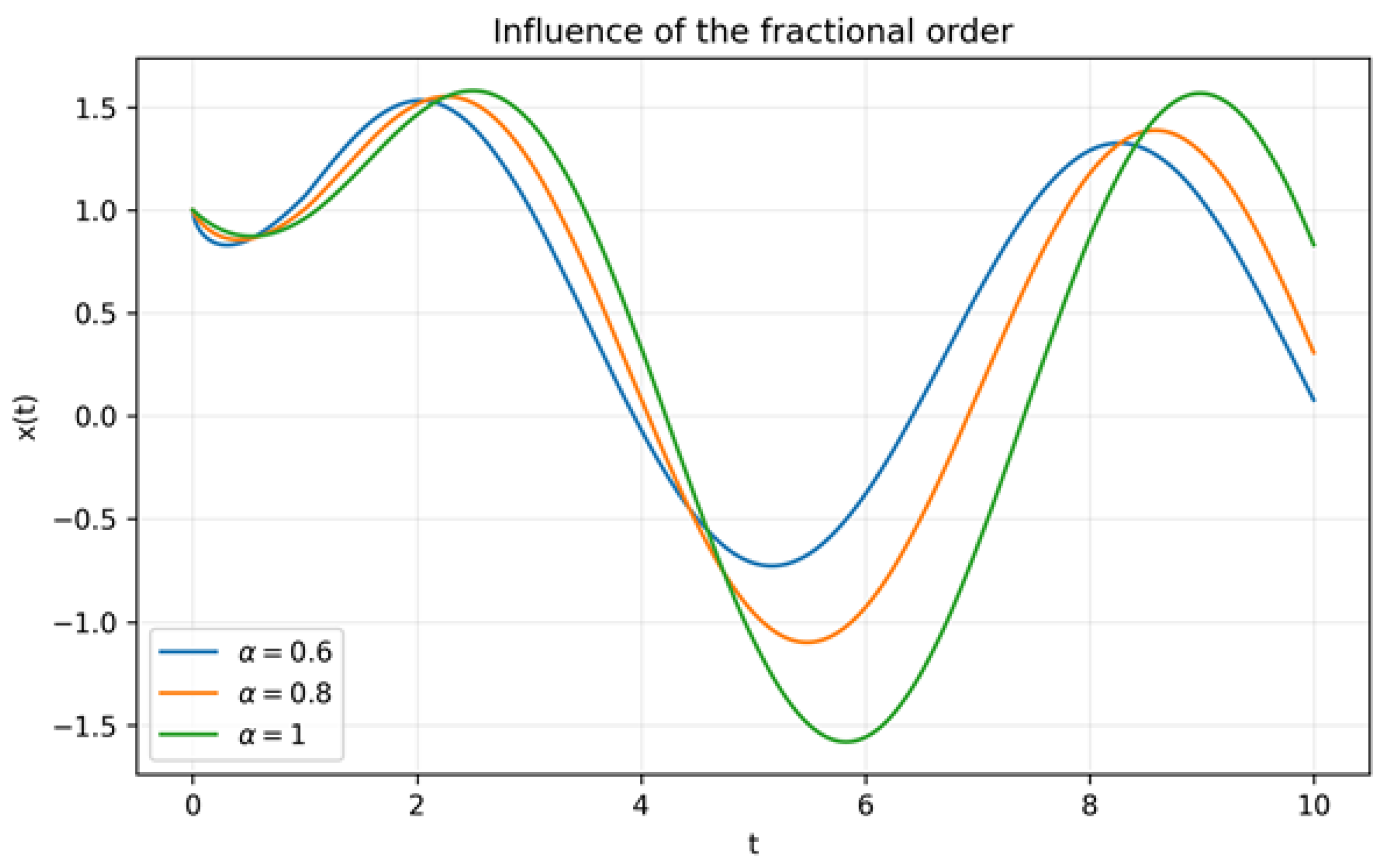The calculations and plots were prepared in R; the complete script is supplied separately. To separately illustrate the influence of the fractional order and the delay parameter, two independent numerical experiments were performed. First, the delay was fixed at $\tau =1$ and the computations were repeated for $\alpha =0.6,0.8$, and 1. The resulting trajectories are presented in Figure 1.

It can be observed that decreasing the fractional order produces a smoother system response and modifies both the phase and amplitude of oscillations. This behavior reflects the long-memory property of the Caputo fractional derivative: the present state depends on the entire history of the solution rather than only on its instantaneous value [44]. 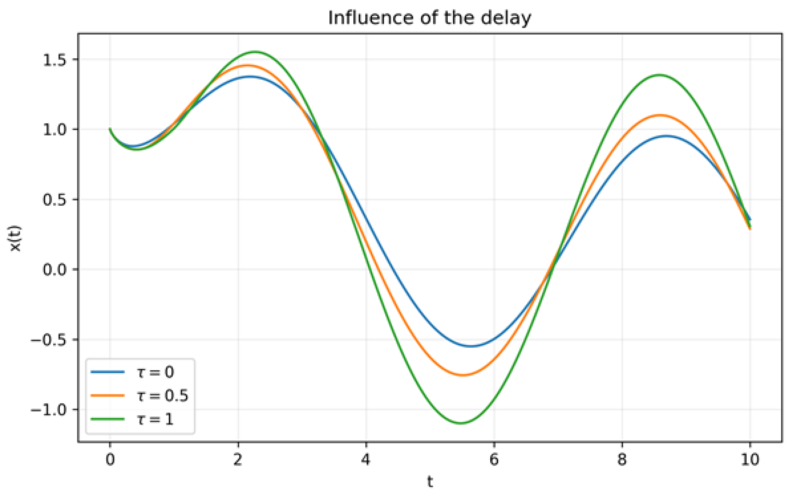Consequently, the dynamics differ noticeably from the classical case $\alpha =1$, illustrating the influence of hereditary effects predicted by the theoretical model. Next, the fractional order was fixed at $\alpha =0.8$, and the delay was varied over $\tau =0,0.5,$ and 1. Figure 2 shows the corresponding numerical trajectories.

Figure 2 demonstrates the influence of the delay parameter on the system trajectory. Increasing the delay changes the interaction between the current and past states, leading to visible phase shifts and modifications of the oscillation amplitude. This confirms that the delay term introduces an additional memory mechanism independent of the fractional derivative, and that both effects jointly determine the qualitative behavior of the solution. Although the numerical experiment concerns a scalar equation and does not constitute a proof of the abstract theorem, it illustrates a finite-dimensional case covered by the general theory and demonstrates how the parameters $\alpha$ and $\tau$ influence an admissible solution trajectory. The numerical results are fully consistent with the theoretical analysis and provide a visual illustration of the existence result established in Theorem 5.

7. Conclusions and Future Research

The main contributions of this paper can be summarized as follows:

1.

We established an existence theorem for pseudosolutions of fractional retarded dynamic equations on arbitrary time scales by combining the $\Delta$-Henstock–Kurzweil–Pettis integral, the De Blasi measure of weak noncompactness, and Kubiaczyk’s fixed point theorem.

2.

We developed a unified analytical framework that simultaneously incorporates fractional dynamics, explicit delay, arbitrary time scales, generalized integration, and weak topological methods, thereby integrating several research directions that have previously been investigated separately.

3.

The obtained existence theorem is formulated under relatively weak assumptions. In particular, compactness of the solution operator is not required; instead, weak sequential continuity together with a condensing-type estimate expressed via the De Blasi measure of weak noncompactness is sufficient.

4.

The use of the $\Delta$-Henstock–Kurzweil–Pettis integral enlarges the class of admissible vector-valued nonlinear operators compared with approaches based on classical Bochner or Pettis integration.

5.

The theoretical analysis is complemented by both an infinite-dimensional example illustrating the applicability of the assumptions of the main theorem and a numerical illustration demonstrating the influence of the fractional order and the delay parameter on the behavior of solution trajectories.

6.

Consequently, the proposed framework provides a unified analytical basis for studying hereditary systems evolving on continuous, discrete, quantum, and hybrid time scales.

Although the present paper establishes a general existence theory for fractional retarded dynamic equations on arbitrary time scales, several important questions remain open. Future research may focus on the following directions:

1.

Establishing uniqueness, continuous dependence on initial data, and stability results under appropriate Lipschitz-type assumptions;

2.

Extending the theory to stochastic, impulsive, neutral, variable-order, and set-valued fractional dynamic equations on time scales;

3.

Investigating controllability, stabilization, observer design, and optimal control problems within the proposed weak topological framework;

4.

Developing numerical methods together with convergence and error analyses for the considered class of equations;

5.

Studying applications to fractional neural networks, cyber-physical systems, and other delayed dynamical models evolving on arbitrary time scales;

6.

Deriving the assumptions of uniform ACG* regularity and equicontinuity directly from natural conditions imposed on the nonlinear operator.