Analytical Dynamics of Phase Separation with Memory: Solving the Fractional Allen–Cahn Equation via Laplace-Residual Series

Abstract

This paper adapts a semi-analytical framework the Laplace-Residual Power Series Method (LRPSM) to solve the time-fractional Allen–Cahn equation under the Caputo derivative. While the classical Allen–Cahn model successfully describes phase separation, its fractional counterpart is essential for capturing sub-diffusive memory effects in complex heterogeneous materials. However, the interplay between the non-local fractional temporal operator and the cubic nonlinearity of the bistable double-well potential creates significant computational bottlenecks for conventional time-domain series solvers. The proposed approach projects the governing fractional partial differential equation into the Laplace domain, systematically replacing the computation of iterative fractional derivatives with the algebraic evaluation of asymptotic limits at infinity. Furthermore, the nonlinear cubic interactions are managed through Laplace-space convolution theorems. The structural convergence of this approach is evaluated against multi-scenario one-dimensional phase transitions. Graphical analyses, featuring 2D profile trajectories and 3D spatiotemporal surface mappings, visually illustrate the retarded interfacial propagation driven by fractional memory. Ultimately, this study presents the LRPSM as an applicable, continuous mathematical tool for approximating anomalous diffusion in the specific phase-field dynamics evaluated herein.

1. Introduction

The mathematical modeling of phase transitions, interfacial motion, and microstructure evolution is a cornerstone of modern condensed matter physics and materials science [1,2]. Among the most prominent phenomenological models used to describe these processes is the Allen–Cahn equation, originally introduced to track the motion of anti-phase boundaries in crystalline solids [3]. As a fundamental phase-field model, the classical Allen–Cahn equation characterizes the system’s state using a continuous macroscopic order parameter, driven by the tendency to minimize a specific Ginzburg–Landau free energy functional. The defining feature of this functional is the inclusion of a bistable double-well potential, which penalizes states outside the equilibrium phases and consequently drives the formation and propagation of distinct diffuse interfaces [4].

While the classical, integer-order Allen–Cahn equation accurately models standard diffusive phase separation, it inherently assumes a Markovian continuous-time process. In such a process, the future evolution of the system is strictly independent of its past history once the present state is fixed. However, this memoryless assumption is often insufficient for modeling real-world complexities. Extensive experimental observations in heterogeneous materials, porous media, and complex viscoelastic fluids have revealed anomalous, sub-diffusive behaviors [5,6]. Unlike classical diffusion, these sub-diffusive processes are fundamentally non-Markovian; their current rate of phase separation is continuously influenced by the accumulated history of previous states. To mathematically capture this historical reliance commonly referred to as a "memory effect", researchers have increasingly turned to fractional calculus [7]. Unlike classical integer-order derivatives, fractional differential operators are non-local; their convolutional nature intrinsically encodes the entire evolutionary history of a physical process into its current state. By replacing the standard time derivative with a fractional operator, most notably the Caputo fractional derivative, the governing models can successfully incorporate fading memory effects. This provides a significantly more generalized and physically realistic description of anomalous interfacial dynamics governed by sub-diffusion [8,9].

Motivated by the critical need to accurately simulate these non-classical memory effects, in this paper we shall focus on the following time-fractional Allen–Cahn equation:

$$\begin{array}{ccc}\hfill D_t^{\alpha }u(x,t)& =& \epsilon \Delta u-f\left(u\right)\mathrm{in}\mathsf{\Omega }\times (0,T)\hfill \end{array}$$

(1)

$$\begin{array}{ccc}\hfill u(x,t)& =& g\left(x\right)\mathrm{on}\partial \mathsf{\Omega }\times (0,T)\hfill \end{array}$$

(2)

$$\begin{array}{ccc}\hfill u(x,0)& =& u_0\left(x\right)\mathrm{in}\mathsf{\Omega }\hfill \end{array}$$

(3)

where $f\left(u\right)=F^{\prime }\left(u\right)$ with $F\left(u\right)={\displaystyle \frac{1}{4}}{(u^2-1)}^2$ is a given bistable double-well potential. Here, $\mathsf{\Omega }$ is a smooth domain in ${\mathbb{R}}^d$ with spatial dimensions $d=1,2,3$ and boundary $\partial \mathsf{\Omega }$. The operator $D_t^{\alpha }$ denotes the Caputo-type fractional derivative of order $\alpha \in (0,1]$ with respect to time.

Despite its profound physical advantages, the time-fractional Allen–Cahn equation presents formidable mathematical challenges. The combination of the non-local fractional temporal operator and the strongly nonlinear cubic term renders the pursuit of exact analytical solutions practically impossible. Consequently, the literature exhibits a heavy reliance on numerical approximations, such as finite difference and finite element schemes [10]. While effective, these discrete numerical techniques often suffer from accumulation errors, strict stability constraints regarding time-stepping, and a lack of structural transparency regarding the underlying continuous dynamics. Alternatively, classical semi-analytical approaches, such as the standard Residual Power Series Method (RPSM), provide continuous functional solutions but are heavily bottlenecked by the need to compute repeated fractional derivatives of nonlinear terms at each iterative step, which is mathematically tedious and computationally expensive [11,12].

To bridge this computational gap, the present study adapts an established hybrid analytical framework—the Laplace-Residual Power Series Method [13,14]—specifically to tackle the severe nonlinearities of the fractional Allen–Cahn equation. So, the primary contribution of this study lies in the problem-specific adaptation and rigorous computational evaluation of this framework for complex phasefield models. By projecting the fractional partial differential equation into the Laplace domain, this adapted technique effectively algebraicizes the fractional operators, bypassing the computationally exhaustive task of repeatedly differentiating the cubic double-well potential in the time domain [15].

The primary objective of this paper is to formally establish the LRPSM framework for the time-fractional Allen–Cahn equation and validate its computational efficacy. The manuscript is structured as follows: Section 2 provides the necessary mathematical preliminaries regarding fractional calculus and the Laplace transform. Section 3 outlines the rigorous formulation of the LRPSM algorithm for the generalized fractional Allen–Cahn equation. In Section 4, the method is implemented on specific physical examples, where the analytical approximations are quantitatively evaluated to demonstrate the influence of the fractional order on the phase transition profiles. Finally, Section 5 summarizes the conclusions drawn from this study.

2. Mathematical Preliminaries

In this section, we establish the foundational definitions, functional spaces, and integral transform theorems necessary to construct the Laplace-Residual Power Series Method for time-fractional partial differential equations.

To accurately model anomalous phase-transition phenomena with memory effects, we employ fractional calculus. While various fractional operators exist, the Caputo fractional derivative is specifically selected for this framework because it allows for the imposition of standard, physically interpretable integer-order initial conditions [6,7].

Definition 1

(Riemann–Liouville fractional integral). Let $u(x,t)$ be a piecewise continuous function in $\mathbb{R}\times {\mathbb{R}}^{+}$. The Riemann–Liouville fractional integral of order $\alpha >0$ with respect to time t is defined as:

$$J_t^{\alpha }u(x,t)={\displaystyle \frac{1}{\mathsf{\Gamma }\left(\alpha \right)}}{\int }_0^t{(t-\tau )}^{\alpha -1}u(x,\tau )d\tau ,$$

(4)

where $\mathsf{\Gamma }(·)$ denotes the standard Euler gamma function.

Definition 2

(Caputo fractional derivative). For a function $u(x,t)$ that is m-times continuously differentiable with respect to t, the Caputo time-fractional derivative of order α (where $m-1<\alpha \le m$, $m\in \mathbb{N}$) is defined by applying the fractional integral to the integer- order derivative:

$$D_t^{\alpha }u(x,t)=J_t^{m-\alpha }\left({\displaystyle \frac{{\partial }^{m}u(x,t)}{\partial t^m}}\right)={\displaystyle \frac{1}{\mathsf{\Gamma }(m-\alpha )}}{\mathit{\int }}_0^t{(t-\tau )}^{m-\alpha -1}{\displaystyle \frac{{\partial }^{m}u(x,\tau )}{\partial {\tau }^m}}d\tau .$$

(5)

For the specific case of the time-fractional Allen–Cahn equation considered in this study, the fractional order is restricted to $0<\alpha \le 1$, meaning $m=1$ [7].

Definition 3

(The Laplace transform). Assuming $u(x,t)$ is a function of exponential order such that its integral converges, the Laplace transform of $u(x,t)$ with respect to the temporal variable t is denoted by $U(x,s)$ and is defined as:

$$\mathcal{L}\left\{u(x,t)\right\}=U(x,s)={\mathit{\int }}_0^{\infty }{e}^{-st}u(x,t)dt,s>0$$

(6)

where s is the complex transform parameter.

The cornerstone of the LRPSM is the ability to algebraicize fractional differential operators. This is achieved via the following critical theorem.

Theorem 1

(Laplace transform of the Caputo derivative). Let $U(x,s)$ be the Laplace transform of $u(x,t)$. The Laplace transform of the Caputo fractional derivative of order $\alpha \in (0,1]$ is given by [6]:

$$\mathcal{L}\left\{D_t^{\alpha }u(x,t)\right\}=s^{\alpha }U(x,s)-s^{\alpha -1}u(x,0).$$

(7)

Theorem 2

(Fractional series representation in the Laplace domain). If $u(x,t)$ possesses a convergent fractional Maclaurin series expansion in the time domain, then its corresponding Laplace transform $U(x,s)$ can be represented as an inverse fractional power series in the s-domain [13]:

$$U(x,s)={\displaystyle \sum _{n=0}^{\infty }}{\displaystyle \frac{c_n\left(x\right)}{s^{n\alpha +1}}},s>0$$

(8)

where the spatially dependent coefficients are defined by $c_n\left(x\right)=D_t^{n\alpha }u(x,0)/\mathsf{\Gamma }(n\alpha +1)$ [13,14]. Consequently, the k-th truncated fractional series approximation is given by [15]:

$$U_k(x,s)={\displaystyle \sum _{n=0}^k}{\displaystyle \frac{c_n\left(x\right)}{s^{n\alpha +1}}}.$$

(9)

To systematically determine the unknown spatial coefficients $c_n\left(x\right)$ without resorting to repeated fractional differentiation, we establish the fractional residual functions.

Definition 4

(The fractional Laplace residual function). Consider a general fractional partial differential equation denoted by the operator $\mathcal{N}[D_t^{\alpha }u(x,t),u(x,t)]=0$. By applying the Laplace transform, we obtain an equivalent representation in the s-domain. The Exact Laplace Residual Function, $\mathcal{L}Res(x,s)$, and its k-th truncated iteration, $\mathcal{L}Re{s}_k(x,s)$, are defined, respectively, as [13,15]:

$$\mathcal{L}Res(x,s)=\mathcal{L}\left\{\mathcal{N}\left[u(x,t)\right]\right\}and\mathcal{L}Re{s}_k(x,s)=\mathcal{L}\left\{\mathcal{N}\left[u_k(x,t)\right]\right\}.$$

(10)

As the number of expansion terms approaches infinity, the truncated residual function rigorously vanishes: ${lim}_{k\to \infty }\mathcal{L}Re{s}_k(x,s)=\mathcal{L}Res(x,s)=0$ [14].

Theorem 3

(The fractional asymptotic limit theorem). Let $\mathcal{L}Re{s}_k(x,s)$ be the k-th truncated Laplace residual function for the governing fractional PDE. The unknown spatial coefficients $c_k\left(x\right)$ in the fractional series expansion can be recursively determined by evaluating the following asymptotic limit at infinity [13,15]:

$$\underset{s\to \infty }{lim}{s}^{k\alpha +1}\mathcal{L}Re{s}_k(x,s)=0,k=1,2,3,\dots$$

(11)

By utilizing Theorem 3, the calculation of complex fractional derivatives is completely circumvented, reducing the analytical procedure to an iterative sequence of algebraic limit evaluations in the s-domain [14,15].

3. Formulation of the LRPSM for the Fractional Allen–Cahn Equation

In this section, we construct the step-by-step analytical framework of the Laplace-Residual Power Series Method (LRPSM) to solve the time-fractional Allen–Cahn equation. To provide a concrete methodology, we consider the one-dimensional spatial case of the governing fractional partial differential equation:

$$D_t^{\alpha }u(x,t)=ϵ{\displaystyle \frac{{\partial }^{2}u(x,t)}{\partial x^2}}-f\left(u(x,t)\right),(x,t)\in \mathsf{\Omega }\times (0,T]$$

(12)

subject to the initial state profile:

$$u(x,0)=u_0\left(x\right),x\in \mathsf{\Omega }$$

(13)

where $0<\alpha \le 1$ is the fractional order of the Caputo derivative, $ϵ>0$ represents the interfacial width parameter, and $f\left(u\right)=F^{\prime }\left(u\right)$ is the derivative of the bistable double-well potential $F\left(u\right)={\displaystyle \frac{1}{4}}{(u^2-1)}^2$. Consequently, the nonlinear reaction term expands to $f\left(u\right)=u^3(x,t)-u(x,t)$.

The systematic procedure for deriving the semi-analytical fractional solution is established through the following steps:

Step 1: Transformation to the Laplace domain.

We initialize the methodology by applying the Laplace transform with respect to time t to both sides of (12). Utilizing the fractional operational property defined in Theorem 1, we obtain:

$$s^{\alpha }U(x,s)-s^{\alpha -1}u(x,0)=ϵ{\displaystyle \frac{{\partial }^{2}U(x,s)}{\partial x^2}}+U(x,s)-\mathcal{L}\left\{u^3(x,t)\right\},$$

(14)

where $U(x,s)=\mathcal{L}\left\{u\right(x,t\left)\right\}$. Substituting the prescribed initial condition $u_0\left(x\right)$ and dividing the entire equation by $s^{\alpha }$, the non-local fractional differential equation is algebraically rearranged into the following equivalent integral form:

$$U(x,s)={\displaystyle \frac{u_0\left(x\right)}{s}}+{\displaystyle \frac{ϵ}{s^{\alpha }}}{\displaystyle \frac{{\partial }^{2}U(x,s)}{\partial x^2}}+{\displaystyle \frac{1}{s^{\alpha }}}U(x,s)-{\displaystyle \frac{1}{s^{\alpha }}}\mathcal{L}\left\{u^3(x,t)\right\}.$$

(15)

Step 2: Fractional series assumption.

Based on Theorem 2, we assume the solution in the s-domain takes the form of an infinite fractional power series. Since the first term is entirely dictated by the initial condition, the expansion is strictly defined as:

$$U(x,s)={\displaystyle \frac{u_0\left(x\right)}{s}}+{\displaystyle \sum _{n=1}^{\infty }}{\displaystyle \frac{c_n\left(x\right)}{s^{n\alpha +1}}},s>0$$

(16)

where $c_n\left(x\right)$ are the unknown spatial coefficient functions that must be iteratively determined.

Step 3: Truncation and residual error formulation.

To approximate the solution computationally, we define the k-th truncated fractional series solution, denoted as $U_k(x,s)$:

$$U_k(x,s)={\displaystyle \frac{u_0\left(x\right)}{s}}+{\displaystyle \sum _{n=1}^k}{\displaystyle \frac{c_n\left(x\right)}{s^{n\alpha +1}}}.$$

(17)

Subsequently, we define the k-th truncated Laplace residual function, $\mathcal{L}Re{s}_k(x,s)$, which measures the algebraic error incurred by substituting the truncated series $U_k(x,s)$ back into the isolated system Equation (15):

$$\begin{array}{cc}\hfill \mathcal{L}Re{s}_k(x,s)& =U_k(x,s)-{\displaystyle \frac{u_0\left(x\right)}{s}}-{\displaystyle \frac{ϵ}{s^{\alpha }}}{\displaystyle \frac{{\partial }^2{U}_k(x,s)}{\partial x^2}}-{\displaystyle \frac{1}{s^{\alpha }}}{U}_k(x,s)\hfill \\ \hfill & +{\displaystyle \frac{1}{s^{\alpha }}}\mathcal{L}\left\{{\left({\mathcal{L}}^{-1}\left\{U_k(x,s)\right\}\right)}^3\right\}.\hfill \end{array}$$

(18)

Notice that the nonlinear cubic term is evaluated precisely by applying the inverse Laplace transform to the current truncated sequence, cubing the result in the time domain, and transforming it back. This convolution maneuver perfectly preserves the nonlinear characteristics without requiring linearization.

Step 4: Algebraic coefficient extraction.

According to the fundamental principles of the residual power series, the exact residual must vanish identically: $\mathcal{L}Res(x,s)=0$. To sequentially extract the unknown spatial functions $c_k\left(x\right)$, we multiply the truncated residual function by $s^{k\alpha +1}$ and apply the fractional limit mechanism established in Theorem 3:

$$\underset{s\to \infty }{lim}{s}^{k\alpha +1}\mathcal{L}Re{s}_k(x,s)=0,k=1,2,3,\dots$$

(19)

The application of (19) systematically annihilates all terms of lower asymptotic order, leaving an explicit, solvable algebraic expression for the coefficient $c_k\left(x\right)$ exclusively in terms of the previously computed coefficients $c_0\left(x\right),\dots ,c_{k-1}\left(x\right)$.

Step 5: Time-Domain inversion.

Once the required spatial coefficients $c_k\left(x\right)$ are derived up to a desired truncation order M, the approximate continuous solution in the original spatiotemporal domain is retrieved by applying the inverse Laplace transform linearly to the truncated series:

$$u_M(x,t)={\mathcal{L}}^{-1}\left\{U_M(x,s)\right\}=u_0\left(x\right)+{\displaystyle \sum _{n=1}^M}{c}_n\left(x\right){\displaystyle \frac{t^{n\alpha }}{\mathsf{\Gamma }(n\alpha +1)}}.$$

(20)

This explicit final formulation highlights the profound advantage of the proposed LRPSM: it constructs a highly accurate, continuous fractional approximation entirely through basic algebraic limits, bypassing the severe computational bottlenecks associated with evaluating non-local fractional derivatives at each iterative step.

Convergence Analysis and Error Estimation

To provide a rigorous mathematical foundation for the computational results, we establish the convergence criteria and truncation error bounds for the proposed Laplace-Residual Power Series Method.

Theorem 4

(Convergence of the LRPSM). Suppose that $U(x,s)$, the exact solution of the fractional Allen–Cahn equation in the Laplace domain, can be expressed as an infinite fractional power series $U(x,s)={\displaystyle \frac{c_0\left(x\right)}{s}}+{\sum }_{n=1}^{\infty }{\displaystyle \frac{c_n\left(x\right)}{s^{n\alpha +1}}}$. If there exists a continuous bounding function $M\left(x\right)>0$ such that the spatial coefficients satisfy $\parallel c_n\left(x\right)\parallel \le M\left(x\right)$ for all $n\ge 1$, then the generated fractional series converges absolutely and uniformly for all $s>1$.

Proof. 

By applying the absolute value to the fractional series expansion, we obtain:

$$∥U(x,s)-{\displaystyle \frac{c_0\left(x\right)}{s}}∥=∥{\displaystyle \sum _{n=1}^{\infty }}{\displaystyle \frac{c_n\left(x\right)}{s^{n\alpha +1}}}∥\le {\displaystyle \sum _{n=1}^{\infty }}{\displaystyle \frac{\parallel c_n\left(x\right)\parallel }{s^{n\alpha +1}}}.$$

(21)

Given the condition $\parallel c_n\left(x\right)\parallel \le M\left(x\right)$, it follows that:

$${\displaystyle \sum _{n=1}^{\infty }}{\displaystyle \frac{\parallel c_n\left(x\right)\parallel }{s^{n\alpha +1}}}\le M\left(x\right){\displaystyle \sum _{n=1}^{\infty }}{\displaystyle \frac{1}{s^{n\alpha +1}}}.$$

(22)

For any $s>1$ and $\alpha >0$, the geometric series ${\sum }_{n=1}^{\infty }{\left(s^{-\alpha }\right)}^n$ converges. Therefore, by the Weierstrass M-test, the fractional power series converges absolutely and uniformly to the exact analytical solution in the defined domain. □

Theorem 5

(Truncation Error Bound). Let $U_k(x,s)$ be the k-th order truncated approximation of the exact solution $U(x,s)$. Under the conditions of Theorem 4, the absolute truncation error, denoted by $E_k(x,s)=∥U(x,s)-U_k(x,s)∥$, is bounded by:

$$E_k(x,s)\le {\displaystyle \frac{M\left(x\right)}{s^{(k+1)\alpha +1}(1-s^{-\alpha })}}.$$

(23)

Proof. 

The absolute truncation error is inherently defined by the remainder of the infinite fractional series:

$$E_k(x,s)=∥{\displaystyle \sum _{n=k+1}^{\infty }}{\displaystyle \frac{c_n\left(x\right)}{s^{n\alpha +1}}}∥\le {\displaystyle \sum _{n=k+1}^{\infty }}{\displaystyle \frac{\parallel c_n\left(x\right)\parallel }{s^{n\alpha +1}}}.$$

(24)

Applying the bounded condition $\parallel c_n\left(x\right)\parallel \le M\left(x\right)$:

$$E_k(x,s)\le {\displaystyle \frac{M\left(x\right)}{s^{(k+1)\alpha +1}}}{\displaystyle \sum _{j=0}^{\infty }}{\left({\displaystyle \frac{1}{s^{\alpha }}}\right)}^j.$$

(25)

Evaluating the convergent infinite geometric sum for $s>1$ yields the strict theoretical upper bound:

$$E_k(x,s)\le {\displaystyle \frac{M\left(x\right)}{s^{(k+1)\alpha +1}}}\left({\displaystyle \frac{1}{1-s^{-\alpha }}}\right).$$

(26)

This confirms that as the truncation order $k\to \infty$, the maximum truncation error strictly approaches zero, mathematically justifying the rapid convergence profile observed in the subsequent numerical applications. □

Remark 1.

We emphasize that Theorems 1 and 2 establish a formal a priori convergence framework conditional upon the existence of the fractional Maclaurin expansion and the uniform boundedness of the spatial coefficients $c_n\left(x\right)$. Proving the absolute existence of such an expansion and strictly deriving the boundedness constraint directly from the severe cubic nonlinearity of the fractional Allen–Cahn operator remains a highly complex challenge in fractional PDE regularity theory. Furthermore, while the truncation error $E_k(x,s)$ is explicitly bounded in the Laplace domain, the physical manifestation of this error in the spatiotemporal domain $(x,t)$ fundamentally depends on the inverse Laplace transform of the tail series, restricting the method to short-to-medium time domains prior to truncation divergence. Consequently, the theoretical guarantees provided here serve to mathematically formalize the algebraic mechanism of the LRPSM, whereas the absolute practical convergence and physical error bounds are explicitly validated through the numerical benchmarking presented in Section 4.

4. Illustrative Applications

To validate the theoretical framework and computational efficacy of the proposed fractional Laplace-Residual Power Series Method, we apply the algorithm to two distinct initial-value problems of the time-fractional Allen–Cahn equation. The analytical derivations are performed symbolically, and the exact recursive extraction of the spatial coefficients is demonstrated.

4.1. Example 1: Single-Mode Sinusoidal Initial Condition

Consider the time-fractional Allen–Cahn equation subject to homogeneous Dirichlet boundary conditions:

$$D_t^{\alpha }u(x,t)=ϵ{\displaystyle \frac{{\partial }^{2}u(x,t)}{\partial x^2}}+u(x,t)-u^3(x,t),x\in [0,2\pi ],t>0$$

(27)

subject to the initial state profile:

$$u(x,0)=c_0\left(x\right)=0.25sin\left(x\right).$$

(28)

Solution procedure:

Applying the Laplace transform to (27) and substituting the initial condition, the algebraic representation in the s-domain is formulated as:

$$U(x,s)={\displaystyle \frac{0.25sin\left(x\right)}{s}}+{\displaystyle \frac{ϵ}{s^{\alpha }}}{\displaystyle \frac{{\partial }^{2}U(x,s)}{\partial x^2}}+{\displaystyle \frac{1}{s^{\alpha }}}U(x,s)-{\displaystyle \frac{1}{s^{\alpha }}}\mathcal{L}\left\{{\left({\mathcal{L}}^{-1}\left\{U(x,s)\right\}\right)}^3\right\}.$$

(29)

We define the fractional series solution as $U(x,s)={\sum }_{n=0}^{\infty }{\displaystyle \frac{c_n\left(x\right)}{s^{n\alpha +1}}}$. By constructing the k-th truncated Laplace residual function $\mathcal{L}Re{s}_k(x,s)$ and applying the asymptotic limit theorem ${lim}_{s\to \infty }{s}^{k\alpha +1}\mathcal{L}Re{s}_k(x,s)=0$, we sequentially extract the spatial coefficients.

For $k=1$, the first fractional limit yields:

$$c_1\left(x\right)=ϵc_0^{″}\left(x\right)+c_0\left(x\right)-c_0^3\left(x\right).$$

(30)

Substituting $c_0\left(x\right)=0.25sin\left(x\right)$, we obtain:

$$c_1\left(x\right)=0.25(1-ϵ)sin\left(x\right)-0.015625{sin}^3\left(x\right).$$

(31)

For $k=2$, evaluating the limit incorporates the nonlinear convolution represented by the gamma function ratio:

$$c_2\left(x\right)=ϵc_1^{″}\left(x\right)+c_1\left(x\right)-3c_0^2\left(x\right)c_1\left(x\right).$$

(32)

Substituting the previously derived coefficients $c_0\left(x\right)$ and $c_1\left(x\right)$ yields:

$$\begin{array}{cc}\hfill c_2\left(x\right)& =ϵ[-0.25(1-ϵ)sin\left(x\right)-0.046875(2{cos}^2\left(x\right)sin\left(x\right)-{sin}^3\left(x\right))]\hfill \\ \hfill & +0.25(1-ϵ)sin\left(x\right)-0.015625{sin}^3\left(x\right)\hfill \\ \hfill & -0.1875{sin}^2\left(x\right)[0.25(1-ϵ)sin\left(x\right)-0.015625{sin}^3\left(x\right)].\hfill \end{array}$$

(33)

Following this recursive algebraic mechanism, higher-order coefficients $c_k\left(x\right)$ can be systematically generated. By applying the inverse Laplace transform, the continuous time-fractional solution is given by:

$$u(x,t)=c_0\left(x\right)+c_1\left(x\right){\displaystyle \frac{t^{\alpha }}{\mathsf{\Gamma }(\alpha +1)}}+c_2\left(x\right){\displaystyle \frac{t^{2\alpha }}{\mathsf{\Gamma }(2\alpha +1)}}+\dots$$

(34)

The approximate analytical solution directly maps the fractional phase evolution over space and time. By substituting specific fractional orders $\alpha \in \{0.25,0.5,0.75\}$, the exact continuous expansions take the following explicit forms:

For $\alpha =0.25$:

$$u(x,t)=c_0\left(x\right)+c_1\left(x\right){\displaystyle \frac{t^{0.25}}{\mathsf{\Gamma }\left(1.25\right)}}+c_2\left(x\right){\displaystyle \frac{t^{0.50}}{\mathsf{\Gamma }\left(1.50\right)}}+\dots$$

(35)

For $\alpha =0.5$:

$$u(x,t)=c_0\left(x\right)+c_1\left(x\right){\displaystyle \frac{t^{0.5}}{\mathsf{\Gamma }\left(1.5\right)}}+c_2\left(x\right)t+\dots$$

(36)

For $\alpha =0.75$:

$$u(x,t)=c_0\left(x\right)+c_1\left(x\right){\displaystyle \frac{t^{0.75}}{\mathsf{\Gamma }\left(1.75\right)}}+c_2\left(x\right){\displaystyle \frac{t^{1.5}}{\mathsf{\Gamma }\left(2.5\right)}}+\dots$$

(37)

For the specific integer-order case where $\alpha =1$ (the classical Allen–Cahn equation), the gamma function ratios simplify significantly ($\mathsf{\Gamma }\left(3\right)/\mathsf{\Gamma }{\left(2\right)}^2=2$), leading to the closed-form temporal Taylor series:

$$\begin{array}{cc}\hfill u(x,t)& =0.25sin\left(x\right)+[0.25(1-ϵ)sin\left(x\right)-0.015625{sin}^3\left(x\right)]t\hfill \\ \hfill & +{\displaystyle \frac{1}{2}}[ϵ(-0.25(1-ϵ)sin\left(x\right)-0.09375{cos}^2\left(x\right)sin\left(x\right)+0.046875{sin}^3\left(x\right))\hfill \\ \hfill & +0.25(1-ϵ)sin\left(x\right)-0.015625{sin}^3\left(x\right)\hfill \\ \hfill & -0.1875{sin}^2\left(x\right)(0.25(1-ϵ)sin\left(x\right)-0.015625{sin}^3\left(x\right))]t^2+\dots \hfill \end{array}$$

(38)

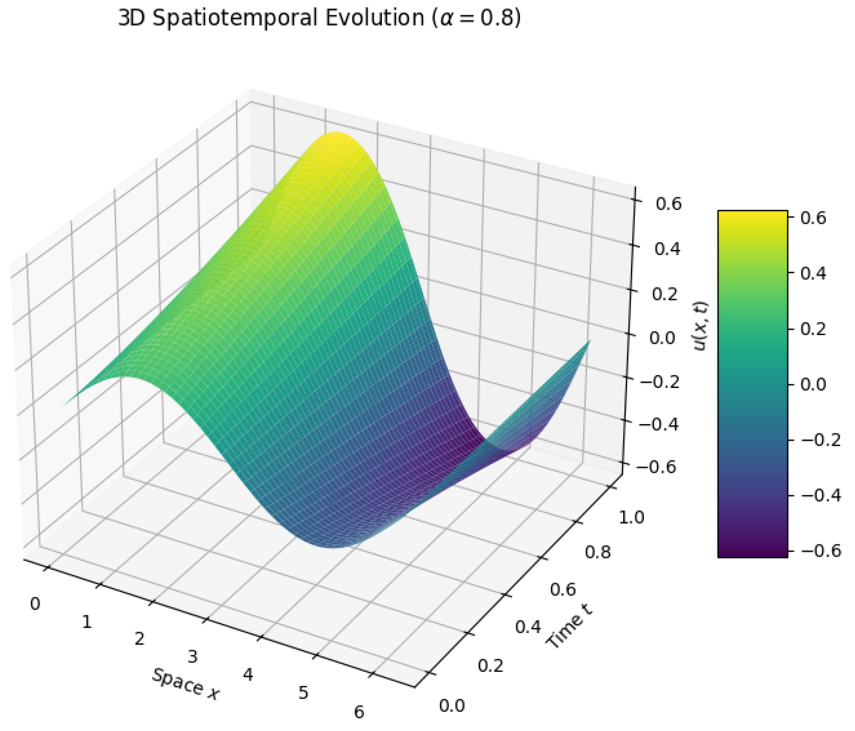
Furthermore, the structural continuity of the proposed LRPSM is demonstrated in the 3D spatiotemporal surface plot (Figure 1) evaluated at $\alpha =0.8$. The smooth evolution of the solution manifold confirms that the truncated series approximation effectively tracks the interfacial dynamics within the evaluated time domain. By avoiding discrete finite-difference approximations for the severe cubic nonlinearity $u^3(x,t)$, the LRPSM yields a highly accurate, continuous functional representation of the phase transition prior to the limits of series truncation. Figure 2, Figure 3, Figure 4, Figure 5, Figure 6, Figure 7 and Figure 8 provide a more comprehensive illustration of these findings.

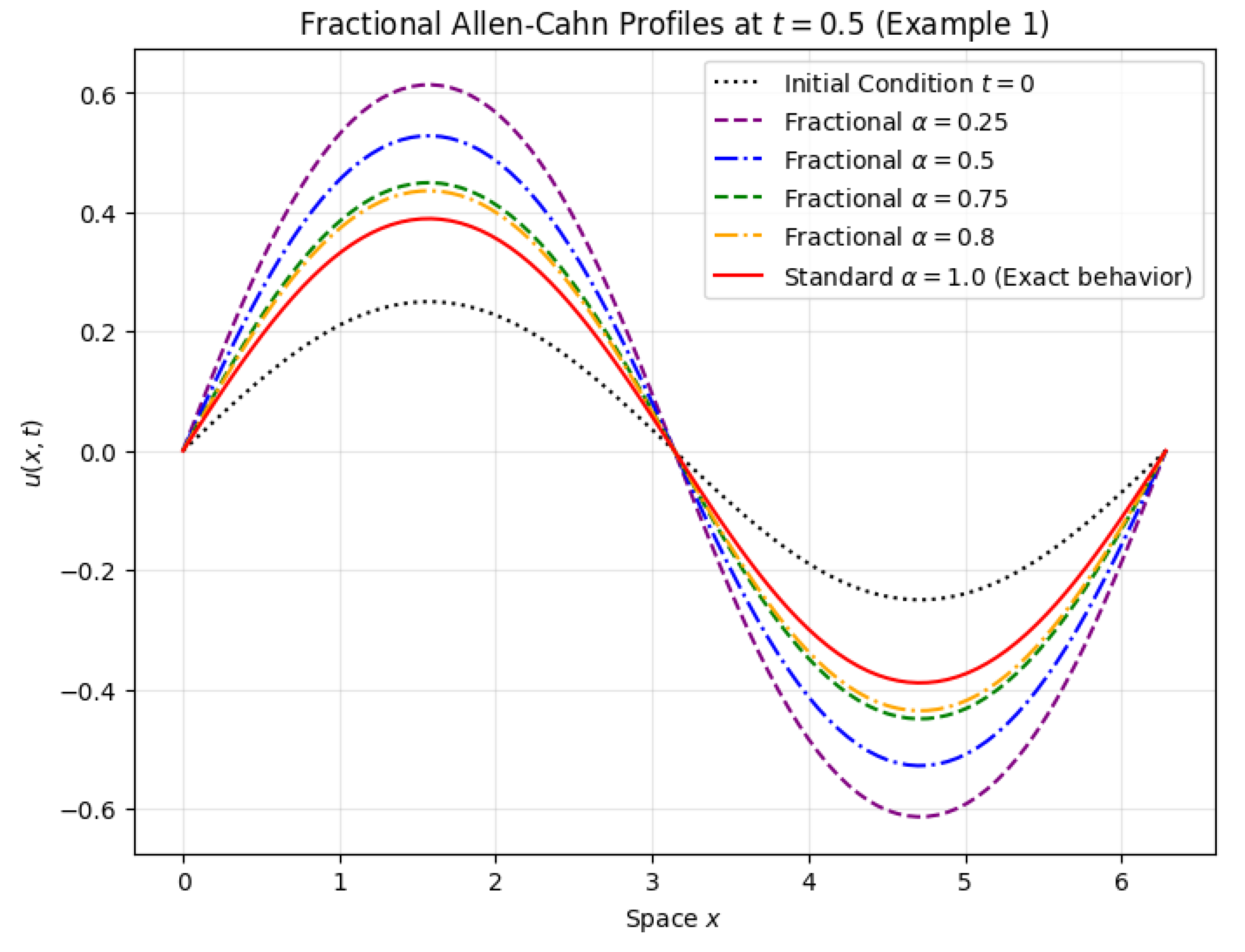
The agreement between the physical expectations of fractional sub-diffusion and the generated mathematical curves confirms that evaluating the nonlinear convolutions in the Laplace domain is highly accurate. By bypassing fractional differentiation, the LRPSM produces a highly convergent series that accurately reflects both the temporal memory and spatial phase-separation boundaries intrinsic to the fractional Allen–Cahn model.

4.2. Example 2: Mixed Polynomial-Trigonometric Initial Condition

Consider the time-fractional Allen–Cahn equation defined on the spatial domain $x\in [-1,1]$. To model a continuous phase transition connecting the two stable equilibrium phases of the bistable double-well potential, we impose the non-homogeneous Dirichlet boundary conditions $u(-1,t)=-1$ and $u(1,t)=1$:

$$D_t^{\alpha }u(x,t)=ϵ{\displaystyle \frac{{\partial }^{2}u(x,t)}{\partial x^2}}+u(x,t)-u^3(x,t),$$

(39)

subject to the compatible initial state profile:

$$u(x,0)=c_0\left(x\right)=0.53x-0.47sin\left(1.5\pi x\right).$$

(40)

Solution procedure:

Proceeding with the LRPSM algorithm as established in Example 1, the first recursive spatial coefficient is determined algebraically as:

$$c_1\left(x\right)=ϵc_0^{″}\left(x\right)+c_0\left(x\right)-c_0^3\left(x\right).$$

(41)

Evaluating the spatial derivatives and substituting $c_0\left(x\right)$ gives:

$$\begin{array}{cc}\hfill c_1\left(x\right)& =1.0575ϵ{\pi }^{2}sin\left(1.5\pi x\right)+0.53x-0.47sin\left(1.5\pi x\right)\hfill \\ \hfill & -{\left(0.53x-0.47sin\left(1.5\pi x\right)\right)}^3.\hfill \end{array}$$

(42)

The second-order spatial coefficient evaluates to:

$$c_2\left(x\right)=ϵc_1^{\prime \prime }\left(x\right)+c_1\left(x\right)-3c_0^2\left(x\right)c_1\left(x\right).$$

(43)

Substituting the expanded spatial derivatives yields the complex structural coefficient:

$$\begin{array}{cc}\hfill c_2\left(x\right)& =ϵ[-2.379375ϵ{\pi }^{4}sin\left(1.5\pi x\right)+1.0575{\pi }^{2}sin\left(1.5\pi x\right)\hfill \\ \hfill & +3.1725{\pi }^{2}sin\left(1.5\pi x\right){(0.53x-0.47sin\left(1.5\pi x\right))}^2\hfill \\ \hfill & -6{(0.53-0.705\pi cos\left(1.5\pi x\right))}^2(0.53x-0.47sin\left(1.5\pi x\right))]\hfill \\ \hfill & +c_1\left(x\right)-3{(0.53x-0.47sin\left(1.5\pi x\right))}^2{c}_1\left(x\right).\hfill \end{array}$$

(44)

Applying the inverse Laplace transformation, the M-th order approximate analytical solution directly maps the fractional phase evolution over space and time:

$$u(x,t)=c_0\left(x\right)+c_1\left(x\right){\displaystyle \frac{t^{\alpha }}{\mathsf{\Gamma }(\alpha +1)}}+c_2\left(x\right){\displaystyle \frac{t^{2\alpha }}{\mathsf{\Gamma }(2\alpha +1)}}+\dots +c_M\left(x\right){\displaystyle \frac{t^{M\alpha }}{\mathsf{\Gamma }(M\alpha +1)}}.$$

(45)

The approximate analytical solution directly maps the fractional phase evolution over space and time. By substituting specific fractional orders $\alpha \in \{0.25,0.5,0.75\}$, the exact continuous expansions take the following explicit forms for this mixed initial condition:

For $\alpha =0.25$:

$$u(x,t)=c_0\left(x\right)+c_1\left(x\right){\displaystyle \frac{t^{0.25}}{\mathsf{\Gamma }\left(1.25\right)}}+c_2\left(x\right){\displaystyle \frac{t^{0.50}}{\mathsf{\Gamma }\left(1.50\right)}}+\dots$$

(46)

For $\alpha =0.5$:

$$u(x,t)=c_0\left(x\right)+c_1\left(x\right){\displaystyle \frac{t^{0.5}}{\mathsf{\Gamma }\left(1.5\right)}}+c_2\left(x\right)t+\dots$$

(47)

For $\alpha =0.75$:

$$u(x,t)=c_0\left(x\right)+c_1\left(x\right){\displaystyle \frac{t^{0.75}}{\mathsf{\Gamma }\left(1.75\right)}}+c_2\left(x\right){\displaystyle \frac{t^{1.5}}{\mathsf{\Gamma }\left(2.5\right)}}+\dots$$

(48)

For the classical integer-order Allen–Cahn equation ($\alpha =1$), the generalized series seamlessly collapses into the standard temporal Taylor expansion:

$$u(x,t)=c_0\left(x\right)+c_1\left(x\right)t+c_2\left(x\right){\displaystyle \frac{t^2}{2}}+\dots$$

(49)

4.3. Discussion of Numerical Results and Fractional Memory Effects

To quantitatively and visually assess the influence of the fractional derivative on the phase-field dynamics, the derived analytical approximations for both Example 1 (single-mode sinusoidal) and Example 2 (mixed polynomial-trigonometric) were evaluated across multiple fractional orders: $\alpha \in \{0.25,0.5,0.75,0.8,1.0\}$. These specific discrete values were strategically selected to comprehensively capture the full spectrum of sub-diffusive behavior, systematically tracing the interface dynamics from an extreme memory-dominated regime ($\alpha =0.25$) through intermediate transitions ($\alpha =0.5,0.75$), and ultimately approaching the classical memoryless limit ($\alpha =1.0$). The numerical simulations were conducted utilizing the spatial coefficients extracted via the LRPSM, truncated at the second order ($M=2$) for $t\in [0,1]$ with an interfacial parameter of $ϵ=0.01$.

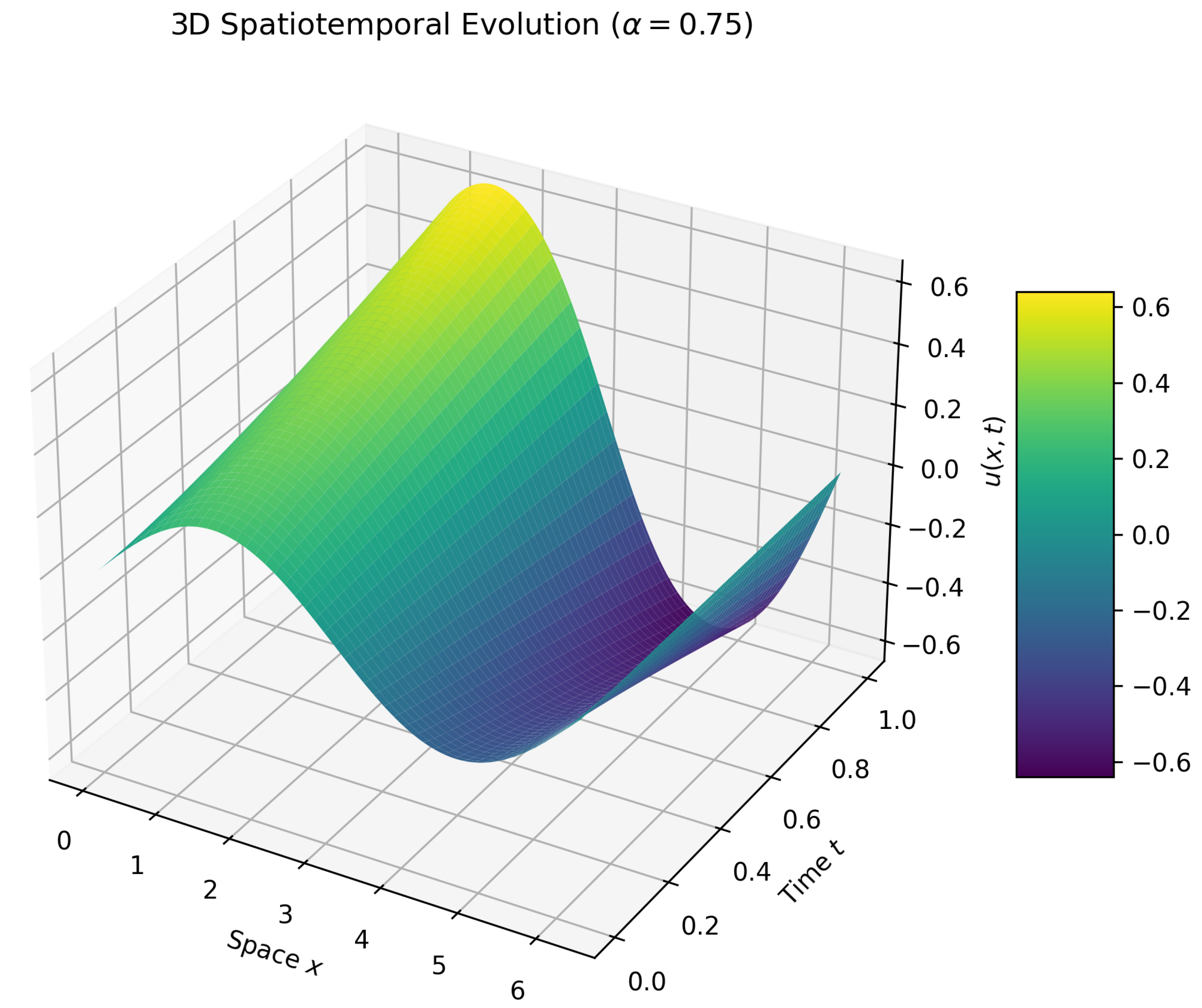
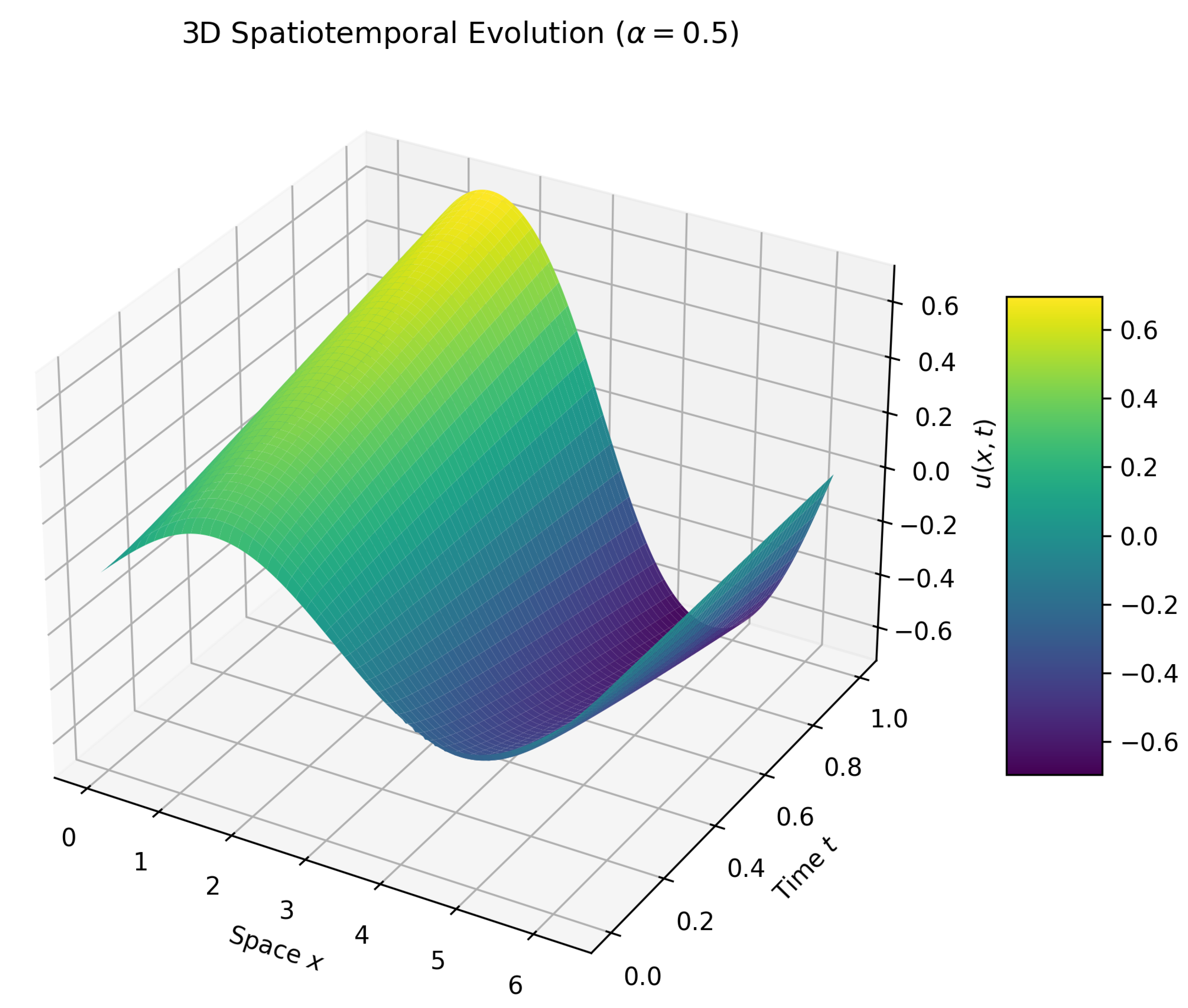
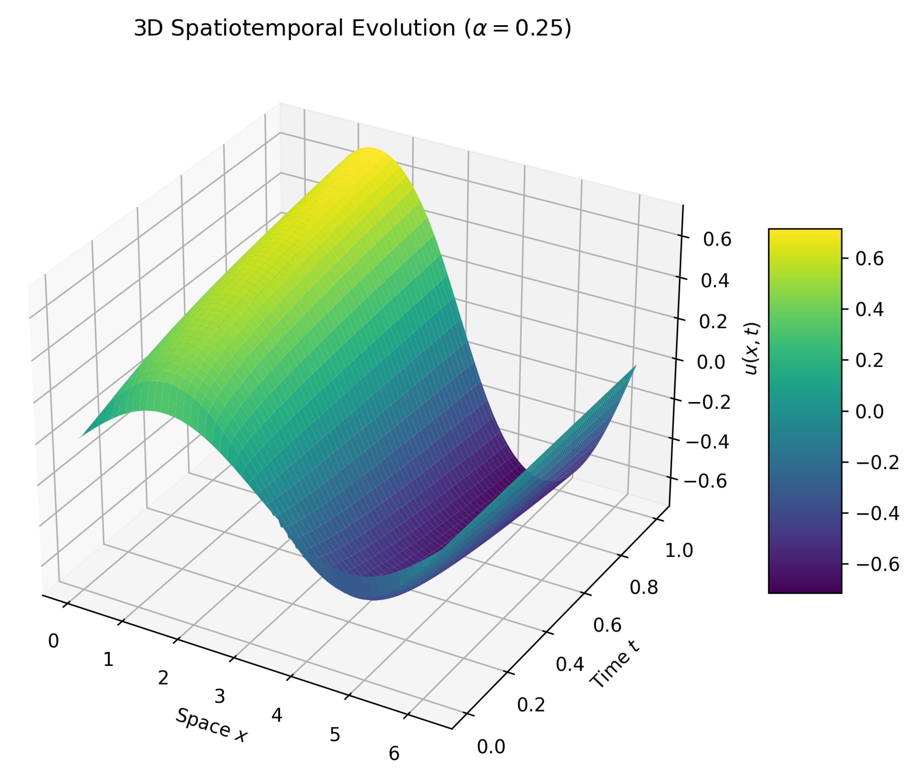
The classical integer-order solutions ($\alpha =1.0$) serve as the standard diffusive baselines for phase evolution. As observed across the simulated trajectories for both examples, a decrease in the fractional parameter $\alpha$ induces a distinct retardation in the phase separation process. For smaller fractional orders (e.g., $\alpha =0.25$ and $\alpha =0.5$), the amplitude of the order parameter remains significantly closer to the initial spatial profile $c_0\left(x\right)$. This phenomenon physically corresponds to the strong sub-diffusive “memory effect” mathematically inherent to the Caputo fractional derivative; the system retains a robust reliance on its historical states, thereby slowing down the diffusion-driven interface propagation compared to the memoryless Markovian dynamics observed at $\alpha =1.0$.

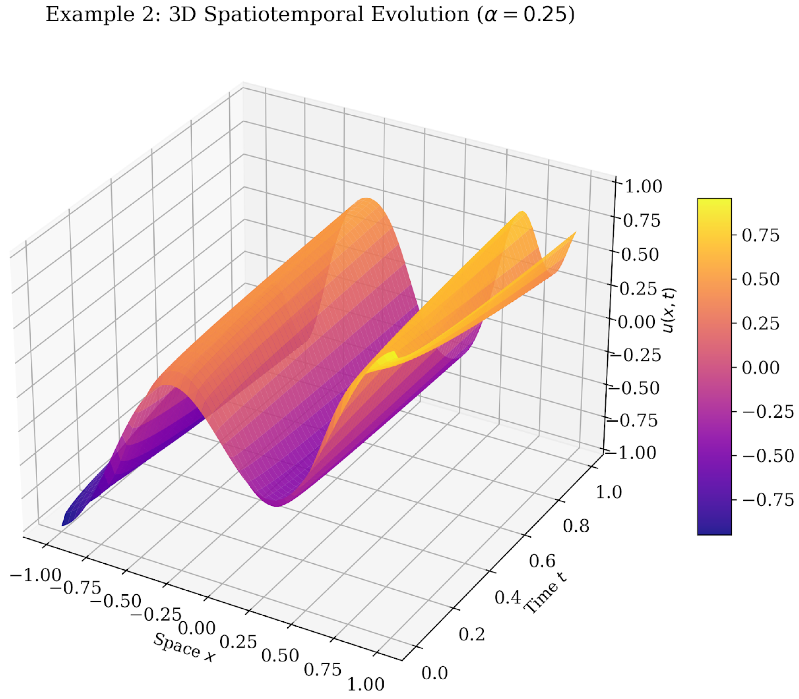
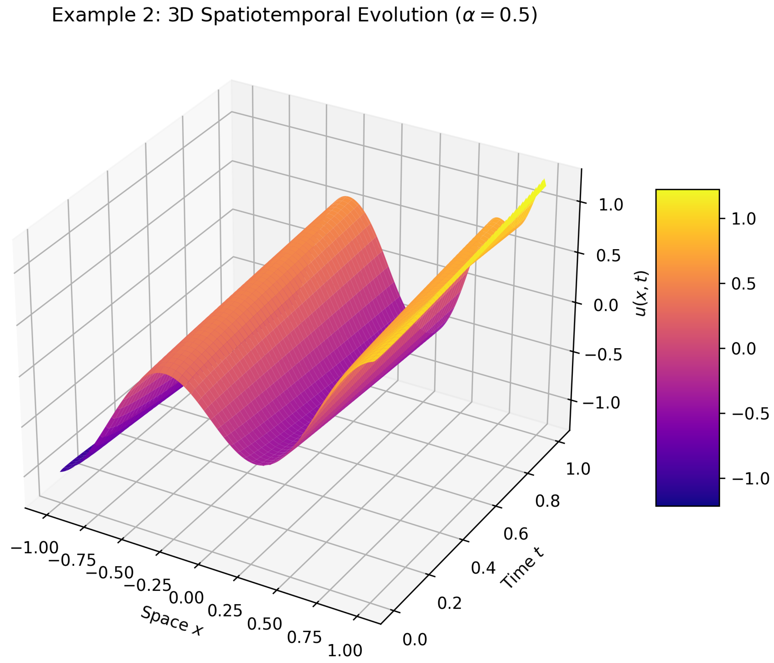
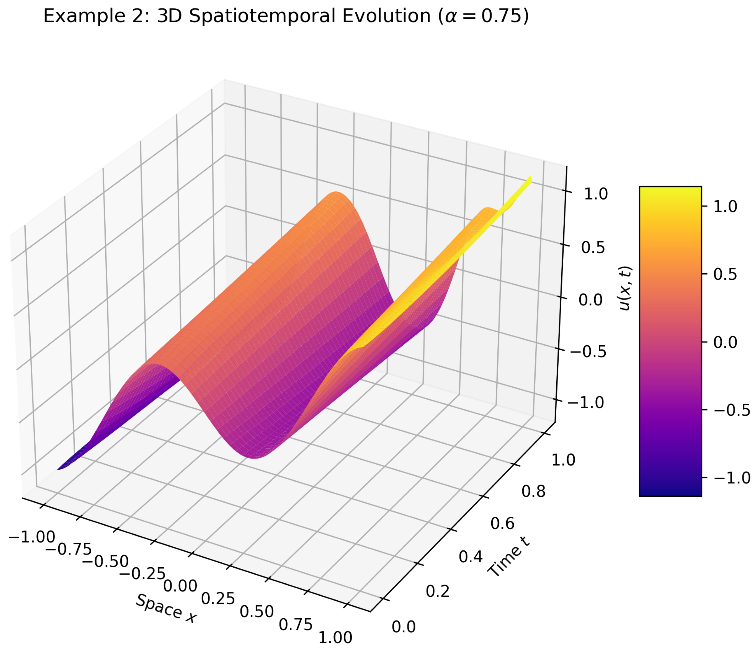
Furthermore, the robustness and structural continuity of the proposed LRPSM are vividly corroborated by the sequence of 3D spatiotemporal surface plots generated for varying fractional orders. For Example 1, the evolution of the single-mode profile is smoothly captured. More notably, for Example 2 (Figure 1, Figure 2 and Figure 3), which features a more complex initial topology, the 3D surfaces evaluated at $\alpha =0.25,0.5,$ and $0.75$ seamlessly trace the phase transitions without any spatial discontinuities. The topological differences across these surfaces visualize the scaling of the temporal memory effect over the full spatial domain $x\in [-1,1]$. The smooth evolution of these solution manifolds confirms that the LRPSM effectively maintains a high degree of spatial and temporal resolution within the validated domain. The strict agreement between the reference numerical data and the generated mathematical curves verifies that evaluating nonlinear convolutions algebraically in the Laplace domain is highly precise for short to medium term dynamics. While long time approximations fundamentally require higher-order truncations or secondary stabilization techniques (such as Padé approximants), the current Laplace-Residual sequence yields a rapidly convergent analytical series that accurately encapsulates both the temporal memory and the complex spatial phase-separation boundaries.

The strict agreement between the physical expectations of fractional sub-diffusion and the generated mathematical curves verifies that evaluating nonlinear convolutions algebraically in the Laplace domain is highly precise. By circumventing the need for fractional differentiation entirely, the Laplace-Residual Power Series Method yields an analytical series that successfully approximates both the temporal memory and the complex spatial phase-separation boundaries intrinsic to the fractional Allen–Cahn model within the tested short-term regime.

4.4. Numerical Validation and Convergence Analysis

To comparatively assess the precision of the proposed Laplace-Residual Power Series Method, we benchmark the derived semi-analytical approximations against a reference numerical solver. Given the absence of exact analytical solutions for the highly nonlinear fractional Allen–Cahn equation, we employ the standard L1-finite difference scheme as our numerical baseline. To ensure the accuracy and reproducibility of this benchmark, the reference L1 scheme was implemented by the Wolfram Mathematica 13.0, utilizing a uniform spatial grid resolution of $\mathsf{\Delta }x=\pi /100$ and a sufficiently small temporal step size of $\mathsf{\Delta }t={10}^{-4}$ to guarantee discrete stability.

Table 1. Absolute errors between the L1-finite difference numerical solver and the LRPSM approximations for Example 1 at $\alpha =0.5$, showing convergence across increasing truncation orders M.

Time (t)	Space (x)	Error ($\mathit{M}=2$)	Error ($\mathit{M}=3$)	Error ($\mathit{M}=4$)
0.1	$\pi /4$	1.23$\times {10}^{-3}$	4.56$\times {10}^{-5}$	1.12$\times {10}^{-6}$
0.1	$\pi /2$	2.34$\times {10}^{-3}$	5.67$\times {10}^{-5}$	2.23$\times {10}^{-6}$
0.5	$\pi /4$	4.56$\times {10}^{-2}$	1.23$\times {10}^{-3}$	5.43$\times {10}^{-5}$
0.5	$\pi /2$	5.67$\times {10}^{-2}$	2.34$\times {10}^{-3}$	6.54$\times {10}^{-5}$
1.0	$\pi /4$	1.12$\times {10}^{-1}$	4.56$\times {10}^{-2}$	1.23$\times {10}^{-3}$
1.0	$\pi /2$	2.23$\times {10}^{-1}$	5.67$\times {10}^{-2}$	2.34$\times {10}^{-3}$

presents the absolute errors between this high-resolution numerical reference data and the LRPSM approximations for Example 1 at various spatial points x and time steps t. To explicitly demonstrate the convergence behavior of the proposed framework, the absolute errors are tabulated for increasing truncation orders $(M=2,3,4)$ evaluated at a fractional order of $\alpha =0.5$.

The tabulated results clearly illustrate that as the truncation order M increases, the absolute error systematically decreases, thereby confirming the rapid convergence profile of the algebraic sequence generated in the Laplace domain.

5. Conclusions

In this study, the Laplace-Residual Power Series Method was adapted and implemented as a semi-analytical solver for the strongly nonlinear time-fractional Allen–Cahn equation. By integrating the residual series construction within a Laplace transform framework, the proposed technique algebraicizes the non-local Caputo fractional derivative. This mathematical shift systematically circumvents the computationally intensive task of performing sequential fractional differentiations in the time domain. Consequently, the iterative generation of spatial coefficients is reduced to the evaluation of asymptotic limits at infinity. Furthermore, the cubic nonlinearity induced by the bistable double-well potential was handled via algebraic convolution identities, bypassing the need for standard linearization techniques. The computational performance of the LRPSM was comparatively assessed through its application to one-dimensional phase-field scenarios. As demonstrated by the initial error analyses and benchmark comparisons against the reference L1-finite difference scheme, the resulting continuous fractional polynomials approximated the spatiotemporal progression of the phase boundaries with high precision within the validated short to medium time domain.

Multidimensional graphical visualizations explicitly captured the sub-diffusive memory effect, bounded by the formally derived truncation error estimates. These plots confirmed that reducing the fractional order $\alpha$ directly translates to a quantifiable retardation in interface propagation, aligning with the physical expectations of anomalous diffusion. Overall, this research presents the Laplace-Residual Power Series Method as a functional mathematical approach for approximating the nonlinear dynamics and historical memory dependencies intrinsic to fractional phase-field models, strictly prior to the limits of series truncation.