Article

Generalized Lipschitz Stability for Switched Differential Equations with Riemann–Liouville Fractional Derivatives with Respect to Another Function


by
Snezhana Hristova
1,* and
Donal O’Regan
2
1
Faculty of Mathematics and Informatics, University of Plovdiv, Tzar Asen 24, 4000 Plovdiv, Bulgaria
2
School of Mathematical and Statistical Sciences, University of Galway, H91 TK33 Galway, Ireland
*
Author to whom correspondence should be addressed.
Fractal Fract. 2026, 10(7), 450; https://doi.org/10.3390/fractalfract10070450
Submission received: 29 March 2026 / Revised: 19 June 2026 / Accepted: 26 June 2026 / Published: 30 June 2026

Abstract

Switched fractional differential equations with Riemann–Liouville fractional derivatives with respect to another function (RLDFs) with orders between zero and one are studied. We provide a detailed algorithm for constructing the solution of the studied switched fractional system, and we illustrate with several examples the influence on both the switching rules and the applied function in the fractional derivative on the behavior of the solution. We define generalized Lipschitz stability in time for the studied system, and this type of stability guarantees that the solutions will be close to the initial values on intervals excluding the points of singularities, i.e., the initial time point and the switching time points. We prove auxiliary results for Lyapunov functions and their RLDFs, including quadratic Lyapunov functions. These results are applied to study generalized Lipschitz stability in time.

1. Introduction

One of the central tasks in the study of fractional differential systems and fractional control is stability analysis; it has been applied mainly to fractional differential systems with Caputo-type derivatives, since they are zero for a constant function and the initial value problem is similar to the Cauchy problem for ordinary differential equations (see, for example, the classical books [1,2] for basic results on Caputo fractional differential equations, as well as some recent results concerning the existence of Caputo–Hadamard differential equations in [3]). However, stability analysis for fractional differential systems with R-L fractional derivatives (RLDs) has recently started being developed (see, for example, [4,5,6,7,8]). In [9], fractional differential equations with the general RLD are investigated, and Laplace convolution is discussed. Note that the analysis of systems involving dual fractional parabolic equations and associated regularity theory can be beneficial in the study of more complex fractional dynamical systems (see, for example [10]). A comprehensive treatment of fractional differential operators and their properties providing additional support for operational calculus used with RLDs can be found in [11], for example.
One type of differential equation that has recently been applied is the category of switching systems. In general, a switched system, generated by a given family of functions, is determined by a switching signal (or switching rule). This is a piecewise constant function whose points of discontinuity are called the switching times. The role of the switching rule is to specify, at each time, the active subsystem from the given family. The switched systems are very interesting in relation to stability. They are well studied for the case of ordinary derivatives (see, for example, [12,13,14]). Furthermore, there are some results in the literature regarding switched fractional differential equations (see [15,16,17]). When the Caputo-type fractional derivative is applied, the main problem is connected to nonlocality in time ([18,19,20,21]). Switched systems with Hilfer fractional derivatives are studied in [22,23,24]. However, to our knowledge, RLDs have not been applied in switched systems. The application of Riemann–Liouville fractional derivatives in switching systems is necessary to model complex physical processes, such as memory effects; to accommodate nonlocal behavior; to achieve a better approximation of real processes; and to describe singularities at some points. If the singularity appears only at the initial time, then we consider the well-known Riemann–Liouville fractional derivative in the fractional differential equation with a continuous right-side part without any switching rule. When the physical process has singularities at points other than the initial point, we must consider the more general case of the Riemann–Liouville fractional derivative with a changing lower limit at every switching point. This requires a separate treatment, especially because of the singular behavior at the initial point and switching times. The presence of singularities requires an appropriate definition of the solution at the switching times. To be as general as possible, we study Riemann–Liouville fractional derivatives with respect to another function.
We address a switched nonlinear system with RLDs if there exist at least two subsystems of fractional-order differential equations to change. To be more general, we use the RLDs with respect to another function (RLDFs) ([1,2,25,26,27]). These types of derivatives have a singularity at the lower limit of the corresponding integral. Unlike integer-order switched models, these equations require updating the RLDFs at each switching time. This leads to singularities at the initial point and switching points, and it makes switched Riemann–Liouville fractional systems more complex than Caputo-based systems. The application of RLDFs to switched systems leads to some difficulties in research. From a practical point of view, it gives us a tool for modeling anomalies in the dynamics of processes.
We give a detailed algorithm for constructing the solution of a switched system with RLDFs. We define generalized Lipschitz stability in time for the studied switched systems with RLDFs. Note that this stability is defined and studied for RLDs in [28]). This stability guarantees the closeness of the solutions to their initial values on intervals excluding the points of singularities (the initial time point and the switching time points). We prove some inequalities for Lyapunov functions and their RLDFs, including quadratic Lyapunov functions, and apply these results as a basis for the study of generalized Lipschitz stability in time, and when the RLDF is applied to a switched system, some particular conditions at switching times are required. Some sufficient conditions are obtained, and some of the theoretical results are illustrated with examples.

2. Preliminary Notes on R-L Fractional Derivatives with Respect to Another Function

Following the results and definitions in Section 2.5 [1] and Section 18.2 [2], we will provide some preliminary results.
We define the following set of functions:
D ( B , P ) = { u C 1 ( [ B , P ] , [ 0 , ) ) : u ( t ) > 0 , t ( B , P ) } ,
where B , P : 0 B < P .
Note that if P = , then [ B , P ] is understood to mean [ B , ) .
Definition 1
((2.5.1) [1], (18.24) [2]). Let the number q > 0 , the function Θ D ( B , T ) and g : [ B , P ] R . The fractional integral with respect to another function (FIF) of the function g is
I B q , Θ g ( t ) = 1 Γ ( q ) B t Θ ( s ) g ( s ) Θ ( t ) Θ ( s ) 1 q d s , t ( B , P ] .
Definition 2
((2.5.17) [1], (18.29) [2]). Let the number q ( 0 , 1 ) , the function Θ D ( B , P ) and g : [ B , P ] R . The R-L fractional derivative with respect to another function (RLDF) of the function g is
D B q , Θ R L g ( t ) = 1 Θ ( t ) d d t I B 1 q , Θ g ( t ) = 1 Θ ( t ) Γ ( 1 q ) d d t B t Θ ( t ) Θ ( s ) q Θ ( s ) g ( s ) d s , t ( B , P ] .
In the case g : [ B , P ] R n , the integral FIF and the derivative RLDF are defined componentwise.
Consider the set
C q ( [ B , P ] , R n , Θ ) = { g C ( [ B , P ] , R n ) : t ( B , P ] D B q , Θ ( t ) R L g ( t ) } .
We will present the result in Theorem 4.1 [25] with slight changes.
Lemma 1.
Let q ( 0 , 1 ) ; Θ D ( B , P ) ; A , y 0 R ; and f C ( [ B , P ] , R ) . Then the solution of the linear fractional differential equation with RLDF
D B q , Θ R L y ( t ) A y ( t ) = f ( t ) , t ( B , P ]
with initial condition
I B 1 q , Θ y ( t ) | t = B = y 0
is given by
y ( t ) = y 0 Θ ( t ) Θ ( B ) q 1 E q , q ( A ( Θ ( t ) Θ ( B ) ) q ) + B t Θ ( t ) Θ ( s ) q 1 E q , q ( A ( Θ ( t ) Θ ( s ) ) q ) f ( s ) Θ ( s ) d s , t ( B , P ] ,
where E q , p ( z ) is the Mittag–Leffler function with two parameters q , p .
In the case A < 0 , note that E q , q ( A ( Θ ( t ) Θ ( B ) ) q ) 1 for t B , and we have the following result:
Corollary 1.
Suppose q ( 0 , 1 ) , Θ D ( B , P ) , y 0 R , A < 0 and f ( t ) 0 . Then the solution y C q ( [ B , P ] , R , Θ ) of (1), (2) satisfies | y ( t ) | | y 0 | Θ ( t ) Θ ( a ) q 1 , t ( B , P ] .
Lemma 2
([1,2]). Let q ( 0 , 1 ) , Θ D ( B , P ) and γ > 1 . Then
I B q , Θ Θ ( t ) Θ ( B ) γ = Γ ( γ + 1 ) Γ ( γ + 1 + q ) Θ ( t ) Θ ( B ) γ + q , t ( B , P ] ,
and
D B q , Θ R L Θ ( t ) Θ ( B ) γ = Γ ( γ + 1 ) Γ ( γ + 1 q ) Θ ( t ) Θ ( B ) γ q , t ( B , P ] .
Corollary 2.
Let q ( 0 , 1 ) , Θ D ( B , P ) , and let A be a constant. Then
D B q , Θ R L Θ ( t ) Θ ( a ) q 1 = 0 , t ( B , P ] ,
and
D B q , Θ R L A = A Γ ( 1 q ) Θ ( t ) Θ ( B ) q , t ( B , P ] .
Remark 1.
In the case Θ ( t ) t , the results of Corollary 2 reduce to Corollary 2.1 and (2.1.20) [1].
Corollary 3.
Let q ( 0 , 1 ) ; Θ D ( B , P ) ; A R ; and
g ( t ) = Θ ( t ) Θ ( B ) q 1 E q , q A Θ ( t ) Θ ( B ) q , t [ B , P ] .
Then
D B q , Θ R L g ( t ) = A g ( t ) , t ( B , P ] .
Proof. 
We note that g ( t ) = k = 0 1 Γ ( q k + q ) A k Θ ( t ) Θ ( B ) k q + q 1 . Take the RLDF on both sides, use Lemma 2 for γ = q k + q 1 and obtain
D B q , Θ R L g ( t ) = k = 0 A k Γ ( q k + q ) D B q , Θ R L Θ ( t ) Θ ( B ) k q + q 1 = k = 0 A k Γ ( q k + q ) Γ ( q k + q ) Γ ( q k ) Θ ( t ) Θ ( B ) q k 1 = A Θ ( t ) Θ ( B ) q 1 k = 0 λ k 1 1 Γ ( q ( k 1 ) + q ) Θ ( t ) Θ ( B ) q ( k 1 ) = A Θ ( t ) Θ ( B q 1 j = 1 A j 1 Γ ( q j + q ) Θ ( t ) Θ ( B ) q j = A Θ ( t ) Θ ( B ) q 1 j = 0 A j 1 Γ ( q j + q ) Θ ( t ) Θ ( B ) q j = A g ( t ) .
Remark 2.
In the case Θ ( t ) t , the result of Corollary 3 reduces to (2.1.54) [1].
The following result is a generalization of Lemma 3.2 [1]:
Lemma 3.
Let q ( 0 , 1 ) , Θ D ( B , P ) and m C q ( [ B , P ] , R , Θ ) .
(a) 
If lim t B + [ ( Θ ( t ) Θ ( B ) ) q 1 m ( t ) ] = c , then
I B 1 q , Θ m ( t ) | t = B : = lim t B + I B 1 q , Θ m ( t ) = c Γ ( q ) .
(b) 
If I B 1 q , Θ m ( t ) | t = B = b and lim t B + [ ( Θ ( t ) Θ ( B ) ) 1 q m ( t ) ] exists, then
lim t B + [ ( Θ ( t ) Θ ( B ) ) 1 q m ( t ) ] = b Γ ( q ) .
Proof. 
Case (a). Let ε > 0 be an arbitrary number. There exists δ > 0 such that
| Θ ( t ) Θ ( B ) 1 q m ( t ) c | < ε 1 Γ ( q ) , t ( B , B + δ ) .
According to Lemma 2, the equality I B 1 q , Θ Θ ( t ) Θ ( B ) q 1 = Γ ( q ) holds, and we obtain
| I B 1 q , Θ m ( t ) c Γ ( q ) | 1 Γ ( 1 q ) B t ( Θ ( t ) Θ ( s ) ) q Θ ( s ) | m ( s ) c ( Θ ( s ) Θ ( a ) ) q 1 d s .
Then, for t ( B , B + δ ) , we have
| I B 1 q , Θ m ( t ) c Γ ( q ) | ε Γ ( q ) Γ ( 1 q ) B t ( Θ ( t ) Θ ( s ) ) q ( Θ ( s ) Θ ( B ) ) q 1 Θ ( s ) d s = ε Γ ( q ) I B 1 q , Θ ( Θ ( s ) Θ ( B ) ) q 1 = ε .
Case (b). The proof follows from Case (a), and we omit it. □
Remark 3.
According to Lemma 3, the initial condition of any fractional differential equation with an RLDF of order q can be expressed in one of the following equivalent forms:
I B 1 q , Θ y ( t ) | t = B + = b
or
lim t B [ ( Θ ( t ) Θ ( B ) ) 1 q y ( t ) ] = b Γ ( q ) ,
where b is a constant.
In our further proofs about stability, we will use some known results about RLDFs:
Lemma 4
(Theorem 2 [4]). Let the function V C ( R n , [ 0 , ) ) , V ( 0 ) = 0 , V ( λ x + ( 1 λ ) y ) λ V ( x ) + ( 1 λ ) V ( y ) for λ [ 0 , 1 ] , x , y R n and the function u C q ( [ B , P ] , R n , Θ ) , u = ( u 1 , u 2 , , u n ) , be such that V ( u ( . ) ) C q ( [ B , P ] , R , Θ ) . Then, the inequality
D B q , Θ R L V ( u ( t ) ) k = 1 n D B q , Θ R L u k ( t ) V ( u ( t ) ) u k , t ( B , P ]
holds.
As special case, we obtain the following result for quadratic functions:
Corollary 4
(Lemma 12 [4]). Let the function u = ( u 1 , u 2 , , u n ) C q ( [ B , P ] , R n , Θ ) be such that u k 2 C q ( [ B , P ] , R , Θ ) , k = 1 , 2 , , n and P R n × n is a positive symmetric square and constant matrix. Then
D B q , Θ R L u T ( t ) P u ( t ) 2 u T ( t ) P D B q , Θ R L u ( t ) , t ( B , P ]
holds.
Now we will prove a result for RLDFs. A similar result for Caputo fractional derivatives with respect to a function is proved in [18].
Lemma 5.
Let q ( 0 , 1 ) , Θ D ( B , P ) , and g C ( [ B , P ] , R ) , and suppose there exists a point η ( B , P ] such that g ( η ) = 0 , g ( t ) < 0 for t [ B , η ) and D η q , Θ R L g ( t ) | t = η exists. Then D B q , Θ R L g ( t ) | t = η 0 .
Proof. 
The functions g ( t ) and Θ ( t ) Θ ( B ) q Θ ( t ) g ( t ) are continuous on [ B , P ] .
For any τ ( B , P ) there exist κ ( τ ) > 0 and h > 0 such that
κ ( τ ) ( Θ ( τ ) Θ ( s ) ) g ( τ ) g ( s ) κ ( τ ) ( Θ ( τ ) Θ ( s ) ) , B < τ h s τ + h < P
and for τ = η we obtain
g ( s ) κ ( η ) ( Θ ( η ) Θ ( s ) ) , η h s η + h .
Define the function H ( t ) = B t Θ ( t ) Θ ( s ) q Θ ( s ) g ( s ) d s , t ( B , P ] . Then
D B q , Θ ( t ) R L g ( t ) | t = η = 1 Θ ( η ) Γ ( 1 q ) d d t H ( t ) | t = η = 1 Θ ( η ) Γ ( 1 q ) lim h 0 H ( η ) H ( η h ) h .
From the definition of the function H ( . ) we obtain
H ( η ) H ( η h ) h = 1 h B η Θ ( η ) Θ ( s ) q Θ ( s ) g ( s ) d s 1 h B η h Θ ( η h ) Θ ( s ) q Θ ( s ) g ( s ) d s = 1 h B η h Θ ( η ) Θ ( s ) q Θ ( η h ) Θ ( s ) q Θ ( s ) g ( s ) d s + 1 h η h η Θ ( η ) Θ ( s ) q Θ ( s ) g ( s ) d s .
The function Θ ( . ) is increasing in [ B , P ] , Θ ( s ) > 0 , s [ B , P ] , q ( 0 , 1 ) , and g ( s ) 0 on [ B , η ] . Then we have Θ ( η ) Θ ( s ) q < Θ ( η h ) Θ ( s ) q , s ( B , η h ) and
B η h Θ ( η ) Θ ( s ) q Θ ( η h ) Θ ( s ) q Θ ( s ) g ( s ) d s 0 .
We can apply inequality (4) and obtain
1 h η h η Θ ( η h ) Θ ( s ) q Θ ( s ) g ( s ) d s κ ( η ) η h η Θ ( η ) Θ ( s ) 1 q d Θ ( s ) = κ ( η ) 2 q Θ ( η ) Θ ( η h ) h 2 q h 1 q .
From inequalities (5), (6) and (7) we obtain
H ( η ) H ( η h ) h κ ( η ) 2 q Θ ( η ) Θ ( η h ) h 2 q h 1 q
or
lim h 0 H ( η ) H ( η h ) h + κ ( η ) 2 q Θ ( η ) Θ ( η h ) h 2 q h 1 q 0 .
Noting 2 q > 0 , 1 q > 0 , we obtain lim h 0 H ( η ) H ( η h ) h 0 , which proves the claim.
Remark 4.
In the special case Θ ( t ) t , the result of Lemma 5 reduces to Lemma 2.3 [29].

3. Description of the Switched Fractional Differential System with RLDF

Let N < , m be given numbers, N = { 0 , 1 , 2 , , N 1 } , M = { 0 , 1 , 2 , , m 1 } . For the family F = { f k C ( [ 0 , ) × R n , R n ) , k N , n < , the sequence of switching times { ξ i } i = 1 m is such that 0 = ξ 0 < ξ 1 < ξ 2 < ξ 3 < < ξ m 1 . If m = , then we assume lim i ξ i = . In this paper, the intervals ( ξ k , ξ k + 1 ] , k M will be considered, and if m < , we will assume ξ m = , such that ( ξ m 1 , ξ m ] denotes ( ξ m 1 , ) .
Let the constants C 0 , C 1 , C 2 , , C m 1 : C k N be chosen such that C k C k 1 for any k = 1 , 2 , , m 1 and the switching rule σ : [ 0 , ) N : σ ( t ) = C k for t [ ξ k , ξ k + 1 ) , k M .
Remark 5.
The switching rule is activated at any switching time ξ k , k = 1 , 2 , , m 1 when the C k th subsystem determined by the function from the set F is applied. Furthermore, the RLDF changes its lower limit at the switching times ξ k , k = 1 , 2 , , m 1 .
Define the set
C q ( [ 0 , ) , R n , Θ ) = i = 0 m 1 C q ( [ ξ i , ξ i + 1 ] , R n , Θ ) .
Consider the system of switched fractional differential equations with RLDF (SDE)
D ξ k q , Θ R L u ( t ) = f σ ( t ) ( t , u ( t ) ) , for t ( ξ k , ξ k + 1 ] , k M ,
with initial condition
lim t 0 u ( t ) = u 0 ,
and switching conditions
lim t ξ k + u ( t ) = u ( ξ k ) Γ ( q ) , k M ,
where u 0 R n and the fractional derivative D ξ k q , Θ R L is defined in Definition 2 with B = ξ k and P = ξ k + 1 .
Remark 6.
The switching condition (10) is equivalent to I ξ k 1 q , Θ u ( t ) | t = ξ k = u ( ξ k ) (see Lemma 3).
Remark 7.
In the case where q 1 , the switching condition (10) reduces to lim t ξ k + u ( t ) = u ( ξ k ) , which guarantees the continuity of the solution at the switching point ξ k .
We introduce the following assumption:
(A).
Assume that for any k M and any initial value ν 0 k R n , the IVP for the system of fractional differential equations with RLDF D ξ k q , Θ R L ν ( t ) = f C k ( t , ν ( t ) ) , t ( ξ k , ξ k + 1 ] and lim t ξ k + ν ( t ) = ν 0 k Γ ( q ) has a unique solution ν C q ( [ ξ k , ξ k + 1 ] , R n , Θ ) .
Remark 8.
In connection with assumption (A), we note that some existence conditions for initial value problems for RLD are given in Theorem 3.3 [1]; for weighted RLDF, see [30].
We will give a detailed description of the IVP for SDE (8)–(10) assuming condition (A) holds.
Let t [ ξ 0 , ξ 1 ] . Since σ ( s ) = C 0 N , s [ 0 , ξ 1 ] , the SDE (8) reduces to the following initial value problem for a system of fractional differential equations with RLDF (IVP)
D 0 q , Θ R L u ( t ) = f C 0 ( t , u ( t ) ) , t ( 0 , ξ 1 ] , lim τ 0 + u ( τ ) = u 0 .
According to assumption (A) with ξ k = 0 , C k = C 0 and v 0 k Γ ( q ) = u 0 , the IVP (11) has a solution u ( 0 ) ( t ) C q ( [ 0 , ξ 1 ] , R n , Θ ) .
At time ξ 1 , σ ( t ) = C 1 N on [ ξ 1 , ξ 2 ) , and the SDE (8) reduces to the following initial value problem for a system of fractional differential equations with RLDF (IVP)
D ξ 1 q , Θ R L u ( t ) = f C 1 ( t , u ( t ) ) , for t ( ξ 1 , ξ 2 ] , lim t ξ 1 + u ( t ) = u ( 0 ) ( ξ 1 ) Γ ( q ) .
According to (A) with ξ k = ξ 1 , C k = C 1 and ν 0 k = u ( 0 ) ( ξ 1 ) , IVP (12) has a unique solution u ( 1 ) ( t ) C q ( [ ξ 1 , ξ 2 ] , R n , Θ ) .
At time ξ 2 , we have σ ( t ) = C 2 N , and SDE (8) reduces to the following initial value problem for a system of fractional differential equations with RLDF (IVP)
D ξ 2 q , Θ R L u ( t ) = f C 2 ( t , u ( t ) ) , for t ( ξ 2 , ξ 3 ] , lim τ ξ 2 + u ( τ ) = u ( 1 ) ( ξ 2 ) Γ ( q ) .
According to (A) with ξ k = ξ 2 , C k = C 2 and ν 0 k = u ( 1 ) ( ξ 2 ) , IVP (13) has an unique solution u ( 2 ) ( t ) C q ( [ ξ 2 , ξ 3 ] , R n , Θ ) .
Continuing this process for k M , we obtain the solution to (8), i.e.,
  • for m < ,
    u ( t ) = u ( 0 ) ( t ) , for t [ 0 , ξ 1 ] , u ( 1 ) ( t ) , for t ( ξ 1 , ξ 2 ] , u ( 2 ) ( t ) , for t ( ξ 2 , ξ 3 ] , u ( m 1 ) ( t ) , for t ( ξ m 1 , ) ;
    for m = ,
    u ( t ) = u ( 0 ) ( t ) , for t [ 0 , ξ 1 ] , u ( 1 ) ( t ) , for t ( ξ 1 , ξ 2 ] , u ( 2 ) ( t ) , for t ( ξ 2 , ξ 3 ] , .
Remark 9.
Quite different from the case of the Caputo-type fractional derivative (see [18]), the solution u ( t ) of SDE (8) is discontinuous at any switching time ξ k , k M .
The suggested algorithm for constructing a solution of IVP for SDEs and the dependence of the behavior of the solution of SDEs on the fractional order, on the applied function in RLDF and on the switching rule are illustrated in Example 1.

4. Stability Analysis for SDEs

We will introduce the definition of a Lipschitz stability for the switched system (8). Note that the presence of the R-L type fractional derivative and its singularity at the initial time (in our case, at the switching times) requires this initial time (or the switching times, respectively) to be excluded (see, for example, [28]).
Definition 3.
The system of switched fractional differential equations with RLDF (8) is globally generalized Lipschitz stable in time if there exist δ i ( 0 , μ ) and T i > ( Θ ( ξ i + 1 ) Θ ( ξ i ) ) q 1 > 0 , i M , such that for any initial value u 0 R n , | | u 0 | | < , we have
| | u ( t , u 0 ) | | T i | | u 0 | | f o r a l l t [ ξ i + δ i , ξ i + 1 ] , i M ,
and in the case m < , the interval [ ξ m 1 + δ m 1 , ξ m ] denotes [ ξ m 1 + δ m 1 , ) .
Remark 10.
In the case where there is not a switching rule, Definition 3 reduces to a definition of globally generalized Lipschitz stability in time (GGLS) for a system with an RLDF, which is studied in [4], and then the inequality (16) for GGLS is satisfied on [ δ , ) , i.e., only the initial time is excluded.
Remark 11.
In the case where there are finite times m < acting on the switching rule, GGLS and inequalities (16) are satisfied on intervals excluding both the initial time and all switching points, i.e., on i = 0 m 2 [ ξ i + δ i , ξ i + 1 ] [ ξ m 1 + δ m 1 , ) .
Definition 3 and Remark 11 are illustrated with an example (see Example 4).
We will now prove some preliminary results that will be used in the study of GGLS.
We will prove the following preliminary result for a switched LFDE.
Lemma 6.
Suppose q ( 0 , 1 ) , y 0 0 , P i R , i M , Θ D ( 0 , ) , and the function y C q ( [ 0 , ) , R , Θ ) satisfies
D ξ i q , Θ R L y ( t ) = P i y ( t ) , t ( ξ i , ξ i + 1 ] , i M , lim t 0 + Θ ( t ) Θ ( 0 ) q 1 y ( t ) = y 0 Γ ( q ) , lim t ξ i + Θ ( t ) Θ ( ξ i ) q 1 y ( t ) = y ( ξ i ) Γ ( q ) , i = 1 , 2 , , m 1 .
Then,
  • for m < ,
    y ( t ) = y 0 Θ ( t ) Θ ( 0 ) q 1 E q , q ( P k ( Θ ( t ) Θ ( 0 ) ) q ) , t ( 0 , ξ 1 ] , y 0 i = 0 k 1 Θ ( ξ i + 1 ) Θ ( ξ i ) q 1 E q , q ( P i ( Θ ( ξ i + 1 ) Θ ( i ) ) q ) × Θ ( t ) Θ ( ξ k ) q 1 E q , q ( P k ( Θ ( t ) Θ ( ξ k ) ) q ) , f o r t ( ξ k , ξ k + 1 ] , k = 1 , 2 , , m 2 , y 0 i = 0 m 2 Θ ( ξ i + 1 ) Θ ( ξ i ) q 1 E q , q ( P i ( Θ ( ξ i + 1 ) Θ ( i ) ) q ) × Θ ( t ) Θ ( ξ m 1 ) q 1 E q , q ( P k ( Θ ( t ) Θ ( ξ m 1 ) ) q ) , t > ξ m 1 ;
    for m = ,
    y ( t ) = y 0 Θ ( t ) Θ ( 0 ) q 1 E q , q ( P k ( Θ ( t ) Θ ( 0 ) ) q ) , t ( 0 , ξ 1 ] , y 0 i = 0 k 1 Θ ( ξ i + 1 ) Θ ( ξ i ) q 1 E q , q ( P i ( Θ ( ξ i + 1 ) Θ ( i ) ) q ) × Θ ( t ) Θ ( ξ k ) q 1 E q , q ( P k ( Θ ( t ) Θ ( ξ k ) ) q ) , f o r t ( ξ k , ξ k + 1 ] , k = 1 , 2 , .
Proof. 
We will apply induction.
Let t ( 0 , ξ 1 ] . According to Lemma 1 with f ( t ) 0 for B = 0 , P = ξ 1 , A = P 0 , we have
y ( t ) = y 0 Θ ( t ) Θ ( 0 ) q 1 E q , q ( P 0 ( Θ ( t ) Θ ( 0 ) ) q ) , t ( 0 , ξ 1 ] .
Consider the interval ( ξ 1 , ξ 2 ] . According to Lemma 1 with f ( t ) 0 for B = ξ 1 , P = ξ 2 , A = P 1 and (20) for t = ξ 1 , we have
y ( t ) = y 0 Θ ( ξ 1 ) Θ ( 0 ) q 1 E q , q ( P 0 Θ ( ξ 1 ) Θ ( 0 ) q ) × Θ ( t ) Θ ( ξ 1 ) q 1 E q , q ( P 1 ( Θ ( t ) Θ ( ξ 1 ) ) q ) , t ( ξ 1 , ξ 2 ] .
By following this procedure, we established the result. □
Corollary 5.
The conditions of Lemma 6 are satisfied when y 0 > 0 . In that case, the solution to LFDE (17) is positive.
We introduce the following assumptions:
Hypothesis 1.
For m = , there exists a number μ > 0 such that inf i M ξ i + 1 ξ i μ .
Hypothesis 2.
For m = , there exists a number ν > 0 such that inf i M Θ ( ξ i + 1 ) Θ ( ξ i ) ν .
Remark 12.
Conditions (H1) and (H2) assume that the time between two consecutive switching acting points never approaches zero and that the difference of the function in the RLDF at two consecutive switching acting points never approaches zero, respectively.
Remark 13.
Let m = and ξ k = k , k M . Then, assumption (H1) is satisfied.
Let m = and Θ ( t ) = e t . Then, Θ ( ξ k + 1 ) Θ ( ξ k ) = e k + 1 e k = e k ( e 1 ) e 1 > 0 , k M , i.e., assumption (H2) is satisfied with ν = e 1 .
Let m = and Θ ( t ) = t t + 1 . Then, Θ ( ξ k + 1 ) Θ ( ξ k ) = k + 1 k + 2 k k + 1 = 1 ( k + 1 ) ( k + 2 ) , k M , i.e., assumption (H2) is not satisfied.
Let m = and Θ ( t ) = t . Then, Θ ( ξ k + 1 ) Θ ( ξ k ) = 1 > 0 , k M , i.e., assumption (H2) is satisfied for ν = 1 .
Lemma 7.
Let m < , q ( 0 , 1 ) , y 0 0 , P i < 0 , i M , and Θ D ( 0 , ) , and let the function y C q ( [ 0 , ) , R , Θ ) be a solution of the switched LFDE (17).
Then, there exist δ i ( 0 , ξ i + 1 ξ i ) , i = 0 , 1 , 2 , , m 2 , δ m 1 > 0 , M i > 0 , i = 0 , 1 , 2 , , m 1 , such that
| y ( t ) | | y 0 | ν k M k , t [ ξ k + δ k , ξ k + 1 ] , k = 0 , 1 , 2 , , m 2 , | y 0 | ν m 1 M m 1 , t > ξ m 1 + δ m 1 ,
where ν = min k = 0 , 1 , 2 , , m 2 Θ ( ξ k + 1 ) Θ ( ξ k ) q 1 > 0 .
Proof. 
According to Lemma 6, equality (18) holds, and by applying E q , q ( z ) 1 Γ ( q ) for z 0 , we obtain
| y ( t ) | | y 0 | 1 Γ ( q ) k + 1 i = 0 k 1 Θ ( ξ i + 1 ) Θ ( ξ i ) q 1 × Θ ( t ) Θ ( ξ k ) q 1 , t ( ξ k , ξ k + 1 ] , k = 0 , 1 , 2 , , m 2 , | y 0 | 1 Γ ( q ) m i = 0 m 2 Θ ( ξ i + 1 ) Θ ( ξ i ) q 1 × Θ ( t ) Θ ( ξ m 1 ) q 1 , t > ξ m 1 .
Denote μ = min k = 0 , 1 , 2 , , m 2 Θ ( ξ k + 1 ) Θ ( ξ k ) > 0 , μ q 1 = ν . Then, Θ ( ξ i + 1 ) Θ ( ξ i ) q 1 μ q 1 = ν , i = 0 , 1 , , m 2 , and we obtain
| y ( t ) | | y 0 | 1 Γ ( q ) k + 1 ν k Θ ( t ) Θ ( ξ k ) q 1 , t ( ξ k , ξ k + 1 ] , k = 0 , 1 , 2 , , m 2 , | y 0 | 1 Γ ( q ) m ν m 1 Θ ( t ) Θ ( ξ m 1 ) q 1 , t > ξ m 1 .
For any k = 0 , 1 , 2 , , m 2 , the function Θ ( t ) Θ ( ξ k ) q 1 decreases on the interval ( ξ k , ξ k + 1 ] , and lim t ξ k Θ ( t ) Θ ( ξ k ) q 1 = . Therefore, there exist δ k ( 0 , ξ k + 1 ξ k ) and M k > Θ ( ξ k + 1 ) Θ ( ξ k ) q 1 > 0 such that the inequality Θ ( t ) Θ ( ξ k ) q 1 < M k holds on [ ξ k + δ k , ξ k + 1 ] , k = 0 , 1 , 2 , , m 2 . The function Θ ( t ) Θ ( ξ m 1 ) q 1 decreases on the interval ( ξ m 1 , ) and lim t ξ m 1 Θ ( t ) Θ ( ξ m 1 ) q 1 = . Therefore, there exist M m 1 > 0 , and δ m 1 > 0 such that Θ ( t ) Θ ( ξ m 1 ) q 1 < M m 1 , t > ξ m 1 + δ m 1 . Then, from (24) noting 1 Γ ( q ) ( 0 , 1 ) , we obtain (22). □
Lemma 7 is illustrated in Example 2.
Lemma 8.
Suppose m = , q ( 0 , 1 ) , y 0 0 , P i < 0 , i M , Θ D ( 0 , ) , the conditions (H1) and (H2) hold and the function y C q ( [ 0 , ) , R , Θ ) satisfies (17).
Then, there exist numbers δ i ( 0 , ξ i + 1 ξ i ) and constants M i > Θ ( ξ i + 1 ) Θ ( ξ i ) q 1 > 0 , i M , such that
| y ( t ) | | y 0 | ν i 1 M i , f o r t [ ξ i + δ i , ξ i + 1 ] , i M ,
where ν = inf k = 0 , 1 , 2 , Θ ( ξ k + 1 ) Θ ( ξ k ) q 1 .
Proof. 
Note that from condition (H2) we have inf k = 0 , 1 , 2 , Θ ( ξ k + 1 ) Θ ( ξ k ) > 0 and ν > 0 . According to Lemma 6, equality (19) holds, and by applying E q , q ( z ) 1 Γ ( q ) < 1 for z 0 and Θ ( ξ i + 1 ) Θ ( ξ i ) q 1 ν , i = 0 , 1 , , we obtain
| y ( t ) | | y 0 | ν k Θ ( t ) Θ ( ξ k ) q 1 , t ( ξ k , ξ k + 1 ] , k = 0 , 1 , 2 , .
For any k = 0 , 1 , 2 , , the function Θ ( t ) Θ ( ξ k ) q 1 decreases on the interval ( ξ k , ξ k + 1 ] and lim t ξ k Θ ( t ) Θ ( ξ k ) q 1 = . Therefore, for any k = 0 , 1 , 2 , , there exist δ k ( 0 , ξ k + 1 ξ k ) and M k > Θ ( ξ k + 1 ) Θ ( ξ k ) q 1 > 0 such that the inequality Θ ( t ) Θ ( ξ k ) q 1 < M k holds on [ ξ k + δ k , ξ k + 1 ] , k = 0 , 1 , 2 , . This proves inequality (25). □
We will prove a comparison result for a switched LFDE.
Lemma 9.
Suppose q ( 0 , 1 ) , y 0 0 , P i R , i M , Θ D ( 0 , ) and the function y C q ( [ 0 , ) , R , Θ ) satisfies the inequalities
D ξ i q , Θ R L y ( t ) P i y ( t ) , t ( ξ i , ξ i + 1 ] , i M , lim t 0 + Θ ( t ) Θ ( 0 ) q 1 y ( t ) y 0 Γ ( q ) , lim t ξ i + Θ ( t ) Θ ( ξ i ) q 1 y ( t ) y ( ξ i ) Γ ( q ) , i = 1 , 2 , , m 1 .
Then, the inequality y ( t ) u ( t ) , t > 0 holds where u C q ( [ 0 , ) , R , Θ ) is a solution of switched LFDE (17).
Proof. 
Note that according to Lemma 6, the function u ( . ) satisfies the equality (18) for m < or (19) for m = .
From there, we apply induction.
Let t ( 0 , ξ 1 ] . From the first and second inequalities in (26), there exist a number δ 0 0 and a function F 0 C ( [ 0 , ξ 1 ] , [ 0 , ) ) such that D 0 q , Θ R L y ( t ) = P 0 y ( t ) F 0 ( t ) , t ( 0 , ξ 1 ] and lim t 0 + Θ ( t ) Θ ( 0 ) q 1 y ( t ) = y 0 δ 0 Γ ( q ) . According to Lemma 1 with B = 0 , P = ξ 1 , and A = P 0 , we have
y ( t ) = ( y 0 δ 0 ) Θ ( t ) Θ ( 0 ) q 1 E q , q ( P 0 ( Θ ( t ) Θ ( 0 ) ) q ) 0 t ( Θ ( t ) Θ ( s ) q 1 E q , q ( P 0 ( Θ ( t ) Θ ( s ) ) q ) F 0 ( s ) Θ ( s ) d s y 0 Θ ( t ) Θ ( 0 ) q 1 E q , q ( P 0 ( Θ ( t ) Θ ( 0 ) ) q ) = u ( t ) , t ( 0 , ξ 1 ] .
Consider the interval ( ξ 1 , ξ 2 ] . From the first and third inequalities in (26), there exist a number δ 1 0 and a function F 1 C ( [ ξ 1 , ξ 2 ] , [ 0 , ) ) such that D ξ 1 q , Θ R L y ( t ) = P 1 y ( t ) F 1 ( t ) , t ( ξ 1 , ξ 2 ] and lim t ξ 1 + Θ ( t ) Θ ( 0 ) q 1 y ( t ) = y ( ξ 1 ) δ 1 Γ ( q ) . According to Lemma 1 with B = ξ 1 , P = ξ 2 , A = P 1 and inequality (27) for t = ξ 1 , we have
y ( t ) = ( y ( ξ 1 ) δ 1 ) Θ ( t ) Θ ( ξ 1 ) q 1 E q , q ( C ( Θ ( t ) Θ ( ξ 1 ) ) q ) + ξ 1 t ( Θ ( t ) Θ ( s ) q 1 E q , q ( P 1 ( Θ ( t ) Θ ( s ) ) q ) F 1 ( s ) Θ ( s ) d s u ( ξ 1 ) Θ ( t ) Θ ( ξ 1 ) q 1 E q , q ( C ( Θ ( t ) Θ ( ξ 1 ) ) q ) = u ( t ) , t ( ξ 1 , ξ 2 ] .
By following this procedure, we establish the result. □
Remark 14.
Note that the second and third inequalities in (26) could be replaced by the equivalent inequalities (see Lemma 3)
I 0 1 q , Θ y ( t ) | t = 0 y 0 , I ξ i 1 q , Θ y ( t ) | t = ξ i y ( ξ i ) i = 1 , 2 , , m 1 .
We define the classes
K = { a C ( [ 0 , ) , [ 0 , ) ) : a ( 0 ) = 0 , a is strictly increasing , a ( r ) K a r for some constant K a > 0 } , L = { a C ( [ 0 , ) , [ 0 , ) ) : a ( 0 ) = 0 , a is strictly increasing , a 1 ( α r ) r α for all r > 0 } .
We will obtain sufficient conditions with Lyapunov functions and their RLDFs in both cases: a finite number of switching times and an infinite number of switching times.
Theorem 1.
Let m < , Θ D ( 0 , ) .
1. 
Suppose f k C ( [ 0 , ) × R n , R n ) , k N , and assumption (A) holds.
2. 
The function V C ( [ 0 , ) × R n , [ 0 , ) ) is such that
(i) 
V ( 0 , u ) a ( | | u | | ) , b ( | | u | | ) V ( t , u ) , u R n , t > 0 , where a K and b L ;
(ii) 
for any function y C q ( [ 0 , ξ 1 ] , R n , Θ ) with lim t 0 + Θ ( t ) Θ ( 0 ) ) 1 q y ( t ) = y 0 Γ ( q ) , | | y 0 | | < , the inequality
lim t 0 + ( Θ ( t ) Θ ( 0 ) ) 1 q V ( t , y ( t ) ) V ( 0 , y 0 ) Γ ( q )
holds;
(iii) 
for any y C q ( [ ξ k , ξ k + 1 ] , R n , Θ ) with lim t ξ k + ( Θ ( t ) Θ ( ξ k ) ) 1 q y ( t ) = y k Γ ( q ) , | | y k | | < , the inequality
lim t ξ k + ( Θ ( t ) Θ ( ξ k ) ) 1 q V ( t , y ( t ) ) V ( t k + 0 , y k ) Γ ( q )
holds;
(iv) 
there exist numbers λ i > 0 , i M such that for any initial value ν 0 R n : | | ν 0 | | < , and the corresponding solution ν ( · ) C q ( [ 0 , ) , R n , Θ ) of (8), the function V ( · , ν ( · ) ) C q ( [ 0 , ) , [ 0 , ) , Θ ) and the inequality
D ξ i q , Θ R L V ( t , ν ( t ) ) λ k V ( t , ν ( t ) ) ) f o r a l l t ( ξ k , ξ k + 1 ] , k M ,
holds and ( ξ m 1 , ξ m ] denotes ( ξ m 1 , ) .
Then, SDE (8) is globally generalized Lipschitz stable in time.
Proof. 
Let u 0 R n , | | u 0 | | < be an arbitrary point. Let u ( . ) C q ( [ 0 , ) , R n , Θ ) be a solution of SDE (8) with initial value u 0 .
Consider the function m ( t ) = V ( t , u ( t ) ) C q ( [ 0 , ) , [ 0 , ) , Θ ) . According to conditions 2(ii), 2(iii) and 2(iv), the function m ( . ) satisfies the inequalities (26) with P i = λ i , y 0 = V ( 0 , u 0 ) , y ( ξ i ) = V ( ξ i , u ( ξ i ) , and i M . According to Lemma 9, we have m ( t ) U ( t ) , t > 0 , where the function U ( . ) C q ( [ 0 , ) , R , Θ ) is a solution of the switched LFDE (17) with P i = λ i , y 0 = V ( 0 , u 0 ) , y ( ξ i ) = V ( ξ i , u ( ξ i ) ) , and i M . According to Corollary 5, the function U ( . ) is positive, and according to Lemma 7, there exist constants δ i ( 0 , ξ i + 1 ξ i ) , i = 0 , 1 , 2 , , m 2 , δ m 1 > 0 , M i > 0 , i = 0 , 1 , 2 , , m 1 , such that | U ( t ) | < V ( 0 , u 0 ) ν k M k , t [ ξ k + δ k , ξ k + 1 ] , k = 0 , 1 , 2 , , m 1 , where ξ m = and the interval [ ξ m 1 + δ m 1 , ξ m ] denotes [ ξ m 1 + δ m 1 , ) .
Therefore,
m ( t ) = V ( t , u ( t ) ) U ( t ) V ( 0 , u 0 ) ν i M i , for t [ ξ i + δ i , ξ i + 1 ] , i M .
From condition 2(i), we have the inequalities for t [ ξ i + δ i , ξ i + 1 ] , i M ,
b ( | | u ( t ) | | ) V ( t , u ( t ) ) V ( 0 , u 0 ) ν i M i ν i M i a ( | | u 0 | | ) V ( 0 , u 0 ) ν i M i K a | | u 0 | | .
From the inclusion b L , we obtain
u r b ( r u ) for all r 0 .
From inequalities (29) and (30) with u = | | u 0 | | , r = Θ i K a ,
b ( | | u ( t ) | | ) ν i M i K a | | u 0 | | b ( ν i M i K a | | u 0 | | ) , for t [ ξ i + δ i , ξ i + 1 ] , i M ,
completing the proof. □
Theorem 2.
Let m = , Θ D ( 0 , ) .
1. 
Suppose f k C ( [ 0 , ) × R n , R n ) ; k N ; and assumptions (A), (H1), and (H2) hold.
2. 
Condition 2 of Theorem 1 is satisfied.
Then SDE (8) is globally generalized Lipschitz stable in time.
The proof is similar to the one in Theorem 1, applying Lemma 8.
Remark 15.
If lim t Θ ( t ) = α > 0 , then assumption (H2) holds and Theorem 2 could be applied.
Remark 16.
In the specific case of Θ ( t ) = t t + 1 and equally spaced switching times ξ k = k A , k = 1 , 2 , , A > 0 , it follows that Θ ( ξ k + 1 ) Θ ( ξ k ) = A ( ( k + 1 ) A + 1 ) ( k A + 1 ) , and assumption (H2) fails; therefore, Theorem 2 does not apply.
In the case of a quadratic function, we obtain the following result.
Theorem 3.
Let m < , Θ D ( 0 , ) .
1. 
Suppose f k C ( [ 0 , ) × R n , R n ) , k N , and assumption (A) holds.
2. 
For any y C q ( [ 0 , ξ 1 ] , R n , Θ ) , y = ( y 1 , y 2 , , y n ) , with
lim t 0 + ( Θ ( t ) Θ ( 0 ) ) 1 q y i ( t ) = y i ( 0 ) Γ ( q ) a n d i = 0 n y i ( 0 ) < ,
the inequalities
lim t 0 + ( Θ ( t ) Θ ( 0 ) ) 1 q ( y i ( t ) ) 2 ( y i ( 0 ) ) 2 Γ ( q ) , i = 1 , 2 , , n ,
hold.
3. 
For any y C q ( [ ξ k , ξ k + 1 ] , R n , Θ ) , y = ( y 1 , y 2 , , y n ) , k M , with
lim t ξ k + Θ ( t ) Θ ( ξ k ) 1 q y i ( t ) = y i ( k ) Γ ( q ) , i = 0 n y i ( k ) < ,
the inequalities
lim t ξ k + ( Θ ( t ) Θ ( ξ k ) ) 1 q ( y i ( t ) ) 2 ( y i ( k ) ) 2 Γ ( q )
hold;
4. 
For any initial value ν 0 R n : | | ν 0 | | < , and the corresponding solution ν ( · ) C q ( [ 0 , ) , R n , Θ ) , ν = ( ν 1 , ν 2 , , ν n ) , of (8), the function i = 1 n ν i 2 ( · ) C q ( [ 0 , ) , [ 0 , ) , Θ ) and the inequality
2 i = 1 n ν i ( t ) f i , ( C k ) ( t , ν ( t ) ) λ i = 1 n ν i ( t ) 2 f o r a l l t ( ξ k , ξ k + 1 ] , k M ,
hold with λ > 0 , and the interval [ ξ m 1 + δ m 1 , ξ m ] denotes [ ξ m 1 + δ m 1 , ) .
Then, SDE (8) is globally generalized Lipschitz stable in time.
The proof follows from Theorem 1 with V ( t , x ) = i = 1 n x i 2 , x = ( x 1 , x 2 , x 3 , , x n ) , and Corollary 4.
Theorem 3 is illustrated in Example 3.
Theorem 4.
Let m = , Θ D ( 0 , ) .
1. 
Suppose f k C ( [ 0 , ) × R n , R n ) ; k N ; and assumptions (A), (H1) and (H2) hold.
2. 
Condition 2 of Theorem 3 is satisfied.
Then, SDE (8) is globally generalized Lipschitz stable in time.
Remark 17.
According to Remark 15, if lim t Θ ( t ) = α > 0 , then assumption (H2) holds, and Theorem 4 can be applied. According to Remark 16, in the specific case Θ ( t ) = t t + 1 and equally spaced switching times ξ k = k A , k = 1 , 2 , , A > 0 , and assumption (H2) fails; therefore, Theorem 4 does not apply.

5. Applications

We will give some examples to illustrate the algorithm for constructing the solution of SGM and the theoretical results.
Example 1.
Let A 0 be a constant, B = 1 and P < .
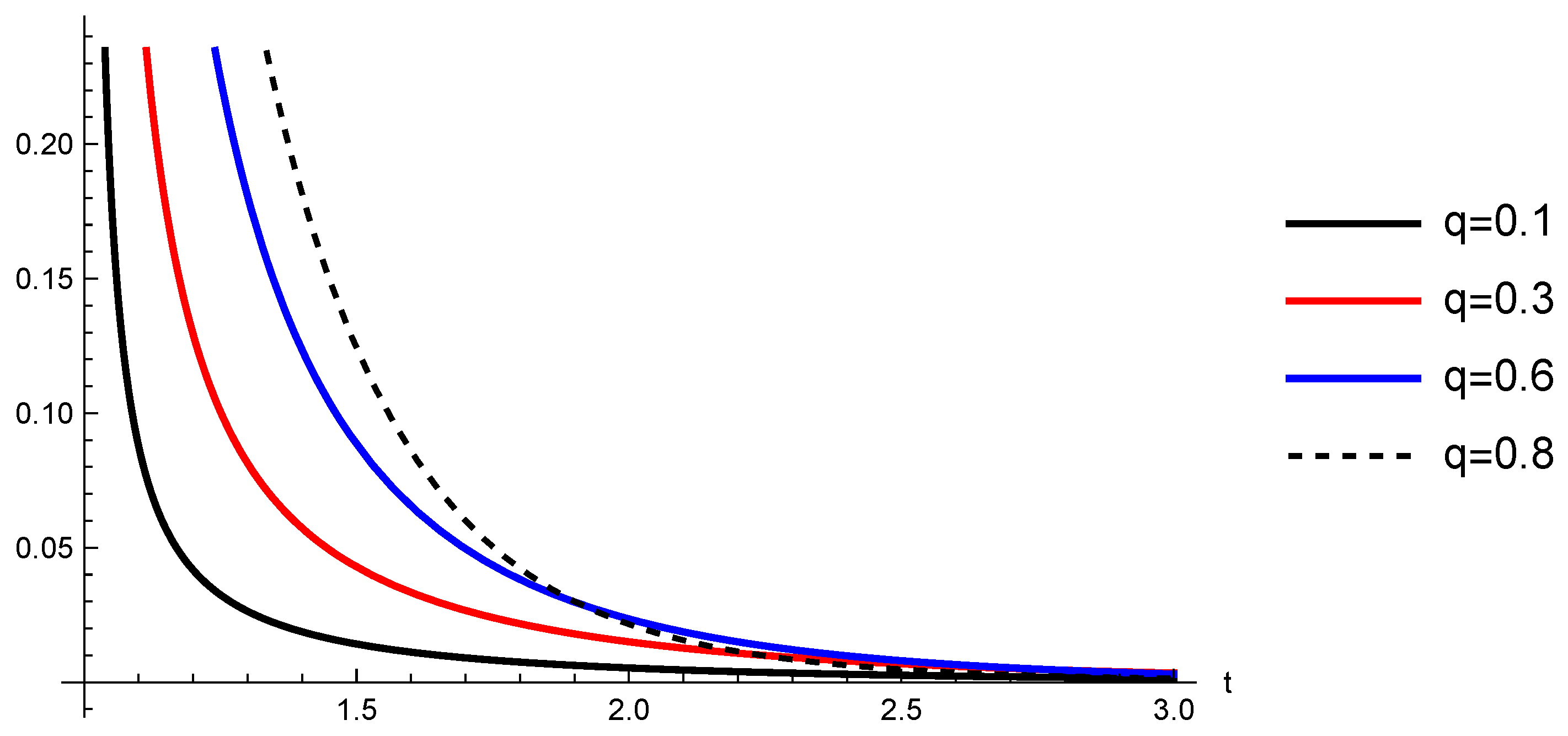
Consider the function h ( t ) = ( Θ ( t ) Θ ( 1 ) ) q 1 E q , q A Θ ( t ) Θ ( 1 ) q (compare to Lemma 1 with f ( t ) 0 ).
Let Θ = e t D ( 1 , T ) . The function h ( t ) is plotted in Figure 1 (with A = 0.2 ) and Figure 2 (with A = 1 ). From both figures, we see that for various values of the fractional order q, the function h(t) approaches zero if the constant A is negative.
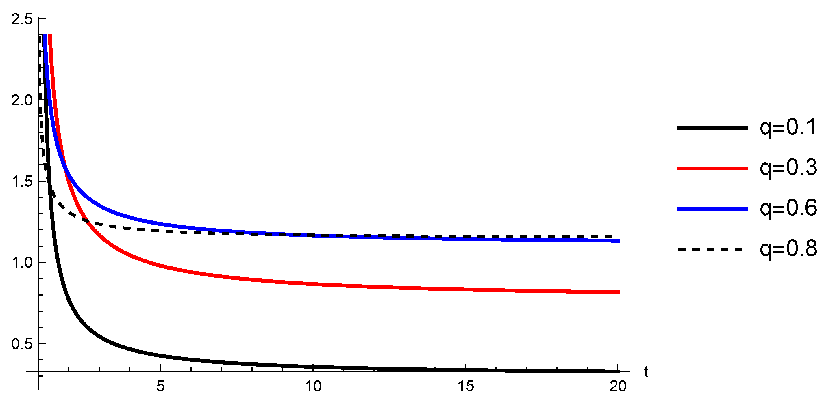
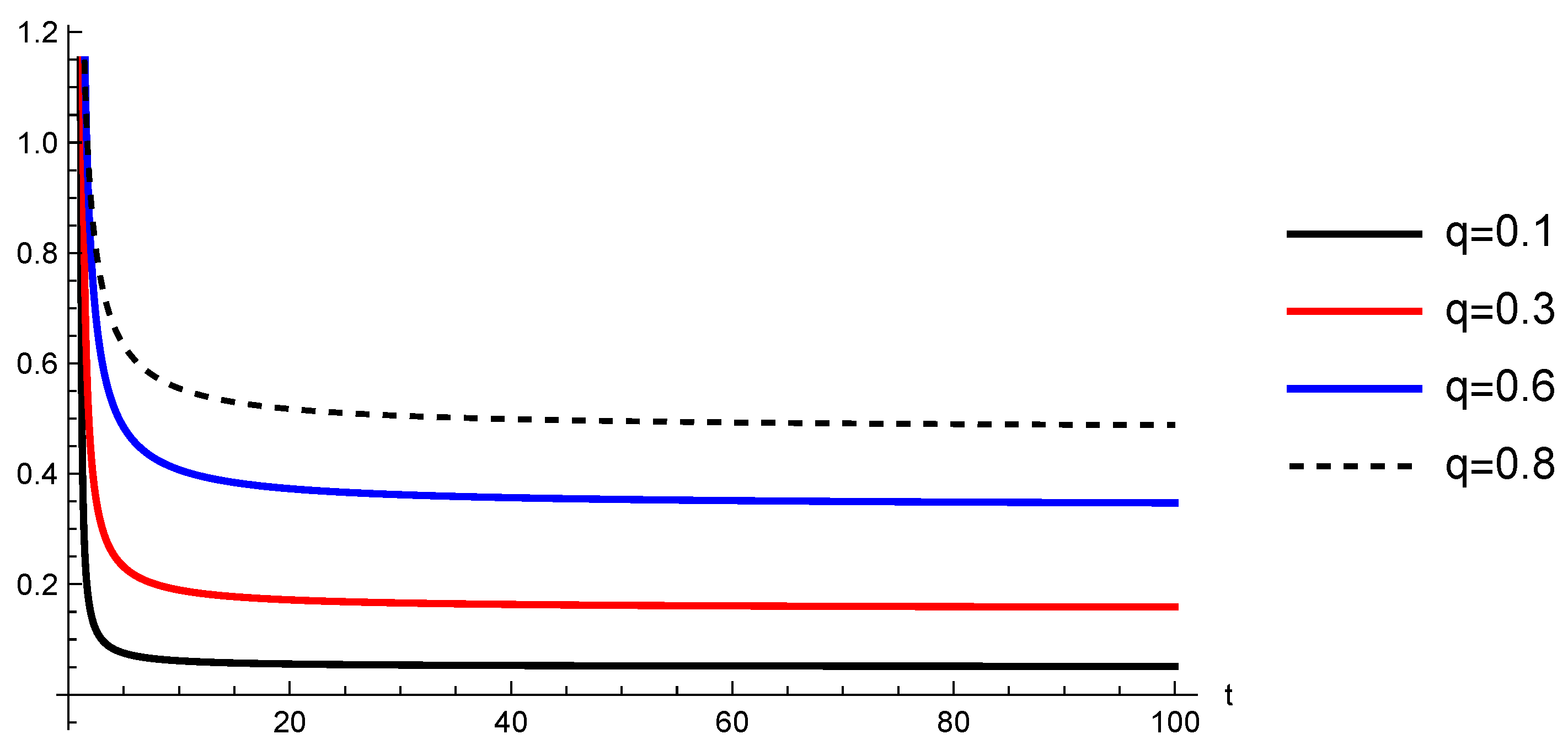
Let Θ = t t + 1 D ( 1 , T ) . The function h ( t ) is plotted in Figure 3 (with A = 0.2 ) and Figure 4 (with A = 1 ). From both figures, we see that for various values of the fractional order q, the function h(t) does not approach zero.
Therefore, the function Θ applied to RLDFs has a massive influence on the behavior of the function h ( t ) .
Now consider the linear scalar fractional differential equation with RLDF (LFDE) (1), (2) with B = 1 , P < , q = 0.3 , and y 0 = 1 . According to Lemma 1 with f ( t ) 0 , its solution is y ( t ) = Θ ( t ) Θ ( a ) 0.3 1 E 0.3 , 0.3 ( A ( Θ ( t ) Θ ( a ) ) q ) for t ( 1 , P ] . If Θ ( t ) = e t D ( 1 , P ) and A = 0.2 , then the solution is increasing and approaching ∞ (see Figure 1). If Θ ( t ) = e t D ( 1 , P ) , A = 1 , then the solution is decreasing and approaching 0 (see Figure 2). If Θ ( t ) = t t + 1 D ( 1 , P ) , A = 0.2 , and q = 0.8 , then the solution is approaching 1.14729 (see Figure 3). If Θ ( t ) = t t + 1 D ( 1 , P ) , A = 1 , q = 0.8 , then the solution is approaching 0.48094 (see Figure 4).
Therefore, the applied function Θ in RLDF has a massive influence on the behavior of the solutions.
Now consider a switched LFDE.
Let N = 2 , i.e., N = { 0 , 1 } , and let the family F of functions consist of two functions f 0 ( t , x ) = 0.2 x and f 1 ( t , x ) = 0.2 x for x R .
Let m = 6 , i.e., M = { 0 , 1 , 2 , 3 , 4 , 5 } . Let the constants C k , k = 0 , 1 , 2 , 3 , 4 , 5 be given such that C k = 0 if k is an even number and C k = 1 if k is an odd number. Let ξ k = k , k = 1 , 2 , 3 , 4 and σ ( t ) = C k , t [ ξ k , ξ k + 1 ) , k = 0 , 1 , 2 , 3 , 4 , 5 . Therefore, at switching times 2 and 4, the switching rule σ ( t ) = 0 is activated and the function f C k ( t , x ) = f 0 ( t , x ) = 0.2 x is applied, and at switching times 1 , 3 , and 5, the switching rule σ ( t ) = 1 is activated and the function f C k ( t , x ) = f 1 ( t , x ) = 0.2 x is applied, i.e., on the intervals ( 0 , 1 ] ( 2 , 3 ] ( 4 , 5 ] , the right-hand side function of the equation is f 0 ( t , x ) = 0.2 x , and on the intervals ( 1 , 2 ] ( 3 , 4 ] ( 5 , ) , the right-hand side function of the equation is f 1 ( t , x ) = 0.2 x .
Then, the switched LFDE will be
D k q , Θ R L u ( t ) = 0.2 u ( t ) , f o r t ( k , k + 1 ] , k = 0 , 2 , 4 , D k q , Θ R L u ( t ) = 0.2 u ( t ) , f o r t ( k , k + 1 ] , k = 1 , 3 , D 5 q , Θ R L u ( t ) = 0.2 u ( t ) , f o r t > 5 , I 0 1 q , Θ u ( t ) | t = 0 = 1 , I k 1 q , Θ u ( t ) | t = k = u ( k 0 ) , k = 1 , 2 , 3 , 4 , 5 .
On the interval ( 0 , 1 ] , we have the following IVP for the LFDE:
D 0 q , Θ R L u ( t ) = 0.2 u ( t ) ) , f o r t ( 0 , 1 ] , I 0 1 q , Θ u ( t ) | t = 0 = 1 .
According to Lemma 1 with f ( t ) 0 , B = 0 , P = 1 , and A = 0.2 , (32) has a solution u ( 0 ) ( t ) = ( Θ ( t ) Θ ( 0 ) ) q 1 E q , q ( 0.2 ( Θ ( t ) Θ ( 0 ) ) q ) , t ( 0 , 1 ] .
On the interval ( 1 , 2 ] , we have the following IVP for the LFDE:
D 1 q , Θ R L u ( t ) = 0.2 u ( t ) , f o r t ( 1 , 2 ] , I 1 1 q , Θ u ( t ) | t = 1 = ( Θ ( 1 ) Θ ( 0 ) ) q 1 E q , q ( 0.2 ( Θ ( 1 ) Θ ( 0 ) ) q ) .
According to Lemma 1 with f ( t ) 0 , B = 1 , P = 2 , and A = 0.2 , (33) has a solution
u ( 1 ) ( t ) = ( Θ ( 1 ) Θ ( 0 ) ) q 1 E q , q ( 0.2 ( Θ ( 1 ) Θ ( 0 ) ) q ) ( Θ ( t ) Θ ( 1 ) ) q 1 × E q , q ( 0.2 ( Θ ( t ) Θ ( 1 ) ) q ) , t ( 1 , 2 ] .
On the interval ( 2 , 3 ] , we have the following IVP for LFDE:
D 2 q , Θ R L u ( t ) = 0.2 u ( t ) ) , f o r t ( 2 , 3 ] , I 2 1 q , Θ u ( t ) | t = 2 = ( Θ ( 1 ) Θ ( 0 ) ) q 1 E q , q ( 0.2 ( Θ ( 1 ) Θ ( 0 ) ) q ) ( Θ ( 2 ) Θ ( 1 ) ) q 1 × E q , q ( 0.2 ( Θ ( 2 ) Θ ( 1 ) ) q ) .
According to Lemma 1 with f ( t ) 0 , B = 2 , P = 3 , A = 0.2 and (34) for t = 2 , (35) has a solution
u ( 2 ) ( t ) = i = 0 1 ( Θ ( i + 1 ) Θ ( i ) ) q 1 E q , q ( ( 1 ) i 0.2 ( Θ ( i + 1 ) Θ ( i ) ) q ) × ( Θ ( t ) Θ ( 2 ) ) q 1 E q , q ( 0.2 ( Θ ( t ) Θ ( 2 ) ) q ) , t ( 2 , 3 ] .
We follow the above procedure inductively to obtain the solution on [ 0 , ) . This solution has a discontinuity at any switching point ( 1 , 2 , 3 , 4 , or 5) because of the switching conditions.
We will consider two different functions applied in the RLDF.
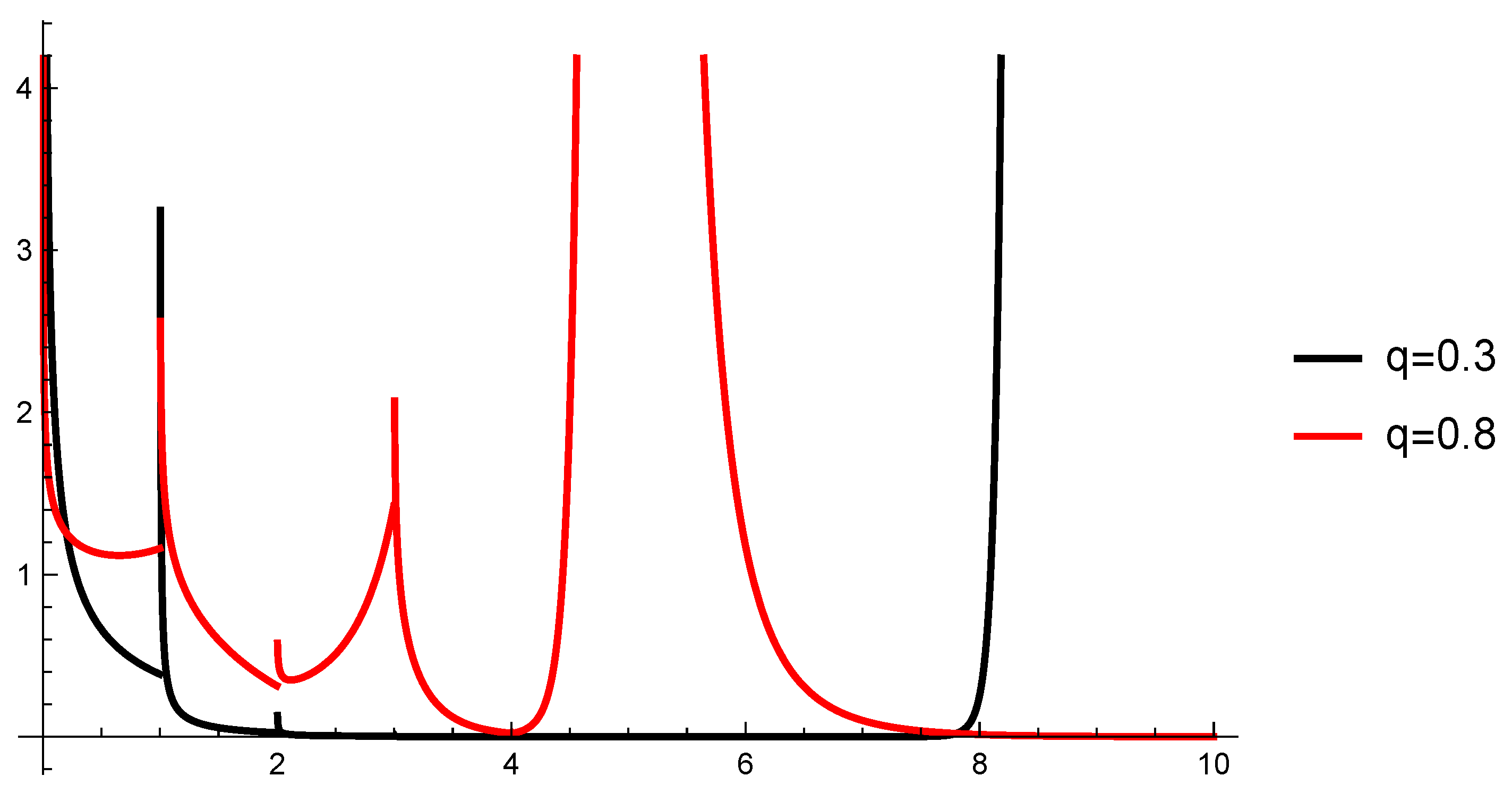
Let Θ ( t ) = e t . The solution of the switched Equation (31) is given by
u ( t ) = i = 0 k 1 ( e i + 1 e i ) q 1 E q , q ( 1 ) i 0.2 ( e i + 1 e i ) q ( e t e k ) q 1 E q , q ( 1 ) k 0.2 ( e t e k ) q , f o r t ( k , k + 1 ] , k = 0 , 1 , 2 , 3 , 4 , i = 0 4 ( e i + 1 e i ) q 1 E q , q ( 1 ) i 0.2 ( e i + 1 e i ) q ( e t e 5 ) q 1 E q , q 0.2 ( e t e 5 ) q , f o r t > 5 .
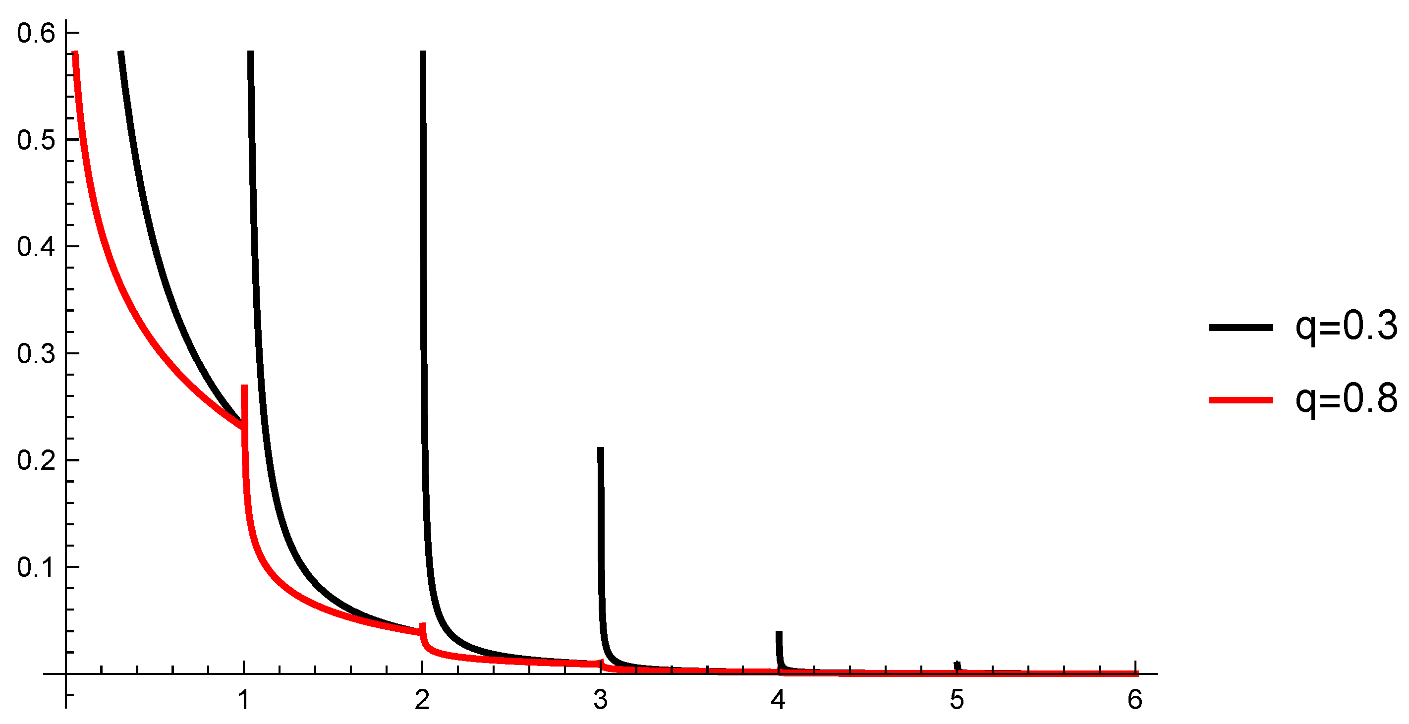
The solution (36) has a discontinuity at the switching points 1 , 2 , 3 , 4 , and 5, and it is graphed in Figure 5. The behavior of the solution of (31) depends on the value of the fractional order. From Figure 5, we can see that if q = 0.8 , then the solution u ( . ) approaches zero, since if q = 0.3 , the solution does not approach zero.
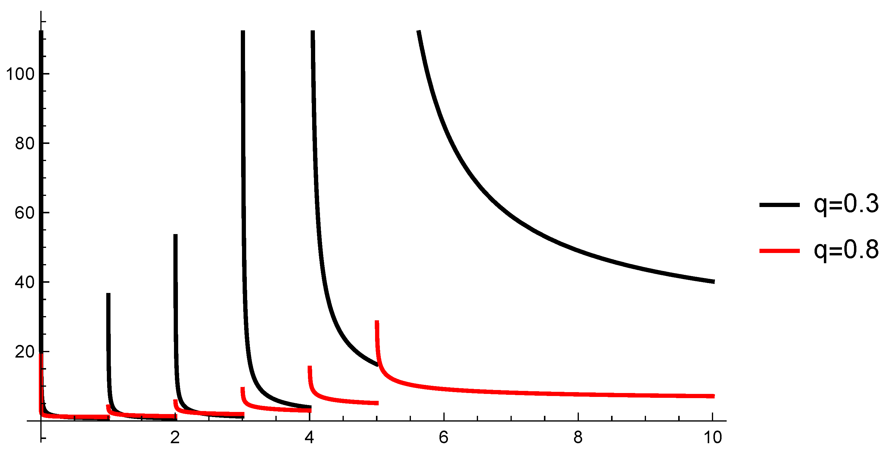
Let Θ ( t ) = t t + 1 . The solution of the switched Equation (31) is given by
u ( t ) = i = 0 k 1 ( i + 1 i + 2 i i + 1 ) q 1 E q , q ( 1 ) i 0.2 ( i + 1 i + 2 i i + 1 ) q ( t t + 1 k k + 1 ) q 1 × E q , q ( 1 ) k 0.2 ( t t + 1 k k + 1 ) q , f o r t ( k , k + 1 ] , k = 0 , 1 , 2 , 3 , 4 , i = 0 4 ( i + 1 i + 2 i i + 1 ) q 1 E q , q ( 1 ) i 0.2 ( i + 1 i + 2 i i + 1 ) q ( k k + 1 5 6 ) q 1 × E q , q 0.2 ( t t + 1 5 6 ) q , f o r t > 5 .
The solution (37) has discontinuities at the switching points 1 , 2 , 3 , 4 , and 5, and it is graphed in Figure 6. Note that the solution does not approach zero for various values of the fractional order q. The solution of the switched Equation (31) has different limits for different values of q.
Therefore, the behavior of the solution depends on the fractional order, on the applied function in the RLDF and on the switching rule.
Example 2.
Consider a switched LFDE with N = 2 , the family F of functions consisting of two functions f 0 ( t , x ) = 0.2 x and f 1 ( t , x ) = 0.4 x for x R .
Let m = 6 , ξ k = k , and k = 1 , 2 , 3 , 4 , 5 ; define the constants C k such that C k = 0 if k is an even number and C k = 1 if k is an odd number; and define the switching rule σ ( t ) = C k , t [ ξ k , ξ k + 1 ) , k = 0 , 1 , 2 , 3 , 4 , 5 . Therefore, at the switching times 2 and 4, the switching rule σ ( t ) = 0 is activated, and the function f C k ( t , x ) = f 0 ( t , x ) = 0.2 x is applied, whereas at switching times 1 , 3 , and 5, the switching rule σ ( t ) = 1 is activated, and the function f C k ( t , x ) = f 1 ( t , x ) = 0.4 x is applied, i.e., on the intervals ( 0 , 1 ] ( 2 , 3 ] ( 4 , 5 ] , the right-hand side function of the equation is f 0 ( t , x ) = 0.2 x , and on the intervals ( 1 , 2 ] ( 3 , 4 ] ( 5 , ) , the right-hand side function of the equation is f 1 ( t , x ) = 0.4 x .
Then the switched system will be
D k q , Θ R L u ( t ) = 0.2 u ( t ) , f o r t ( k , k + 1 ] , k = 0 , 2 , 4 , D k q , Θ R L u ( t ) = 0.4 u ( t ) , f o r t ( k , k + 1 ] , k = 1 , 3 , D 5 q , Θ R L u ( t ) = 0.4 u ( t ) , f o r t > 5 , I 0 1 q , Θ u ( t ) | t = 0 = 1 , I k 1 q , Θ u ( t ) | t = k = u ( k 0 ) , k = 1 , 2 , 3 , 4 , 5 .
All conditions of Lemma 7 are satisfied, and therefore the inequalities (22) hold.
We will consider three different functions applied in the RLDF to illustrate the claim of Lemma 7.
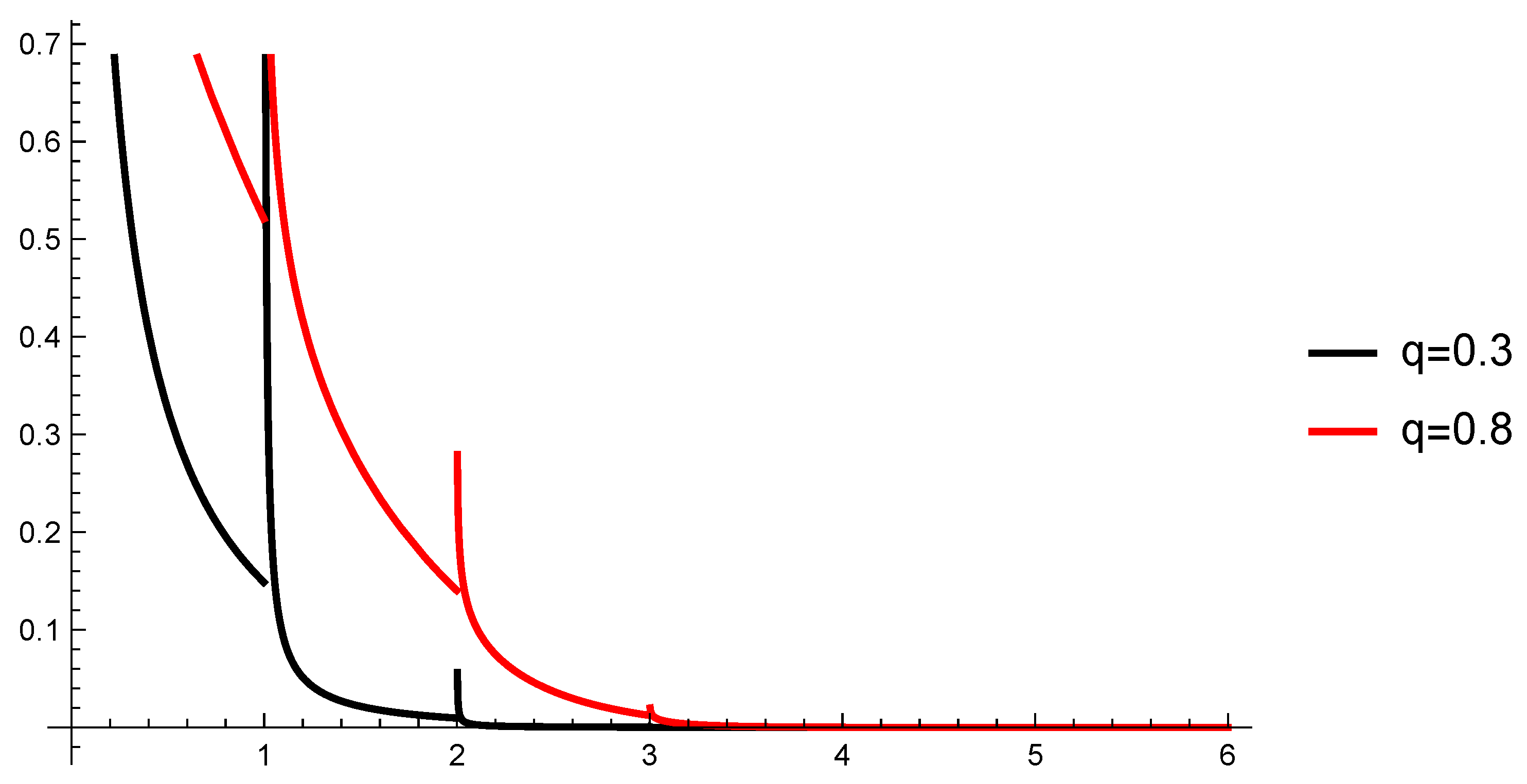
Let Θ ( t ) = e t . The solution to the switched system (38) is given by
u ( t ) = i = 0 k 1 ( e i + 1 e i ) q 1 E q , q ( α i ( e i + 1 e i ) q ) ) ( e t e k ) q 1 E q , q α k ( e t e k ) q , f o r t ( k , k + 1 ] , k = 0 , 1 , 2 , 3 , 4 , i = 0 4 ( e i + 1 e i ) q 1 E q , q α i ( e i + 1 e i ) q ( e t e 5 ) q 1 E q , q 0.4 ( e t e 5 ) q × E q , q 0.2 ( t t + 1 5 6 ) q , f o r t > 5 .
with
α i = 0.2 f o r i e v e n , 0.4 f o r i o d d .
The solution (39) has discontinuities at the switching points 1 , 2 , 3 , 4 , and 5, and it is graphed in Figure 7. The solution approaches zero for the applied fractional orders q.
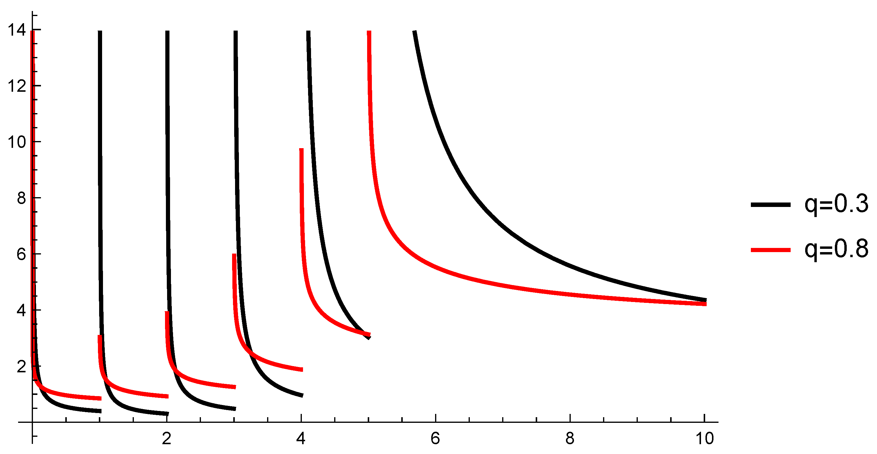
Let Θ ( t ) = t t + 1 . The solution of (38) is given by
u ( t ) = i = 0 k 1 ( i + 1 i + 2 i i + 1 ) q 1 E q , q α i ( i + 1 i + 2 i i + 1 ) q × ( t t + 1 k k + 1 ) q 1 E q , q α k ( t t + 1 k k + 1 ) q , f o r t ( k , k + 1 ] , k = 0 , 1 , 2 , 3 , 4 , i = 0 4 ( i + 1 i + 2 i i + 1 ) q 1 E q , q α i ( i + 1 i + 2 i i + 1 ) q × ( t t + 1 5 6 ) q 1 E q , q 0.4 ( t t + 1 5 6 ) q , f o r t > 5 .
The solution (40) has discontinuities at the switching points 1 , 2 , 3 , 4 , and 5, and it is graphed in Figure 8. The solution (40) does not approach zero.
In the case Θ ( t ) t , the RLDF coincides with the RLD, and the solution of the switched system with RLD (38) is given by
u ( t ) = i = 0 k 1 E q , q ( α i ) ( t k ) q 1 E q , q ( α k ( t k ) q ) ) f o r t ( k , k + 1 ] , k = 0 , 1 , 2 , 3 , 4 , i = 0 4 E q , q ( α i ) ( t 5 ) q 1 E q , q ( 0.4 ( t 5 ) q , f o r t > 5 .
The solution (41) has discontinuities at the switching points 1 , 2 , 3 , 4 , and 5, and it is graphed in Figure 9. In this case, the solution (41) approaches zero for both applied fractional orders.
Therefore, the behavior of the solution of the switched equation depends significantly on the function applied in the RLDF as well as the fractional order.
Example 3.
Consider Example 2. The conditions of Theorem 3 are satisfied, and therefore, SDE (38) is globally generalized Lipschitz stable in time.
For example, for Θ ( t ) = t t + 1 , q = 0.8 (see Figure 8) the constants δ 0 = 0.058 , T 0 = 1.5 , δ 1 = 0.0084 , T 1 = 2.5 , δ 2 = 0.00276 , T 2 = 4 , δ 3 = 0.00754 , T 3 = 5 , δ 4 = 0.035 , T 4 = 6 , δ 5 = 0.05 , and T 5 = 10 , i.e., the solution u ( . ) of SDE (38) satisfies the inequalities (see Figure 8)
| u ( t ) | 1.5 | u 0 | , t [ 0.058 , 1 ] , | u ( t ) | 2.5 | u 0 | , t [ 1.00754 , 2 ] , | u ( t ) | 4 | u 0 | , t [ 2.00276 , 3 ] , | u ( t ) | 5 | u 0 | , t [ 3.00754 , 4 ] , | u ( t ) | 6 | u 0 | , t [ 4.035 , 5 ] , | u ( t ) | 10 | u 0 | , t 0.55 .
Note that the constants T i > ( Θ ( ξ i + 1 Θ ( ξ i ) ) q 1 , i M , depend significantly on the switching points ξ i , on the applied function Θ, and on the fractional order q.
We will illustrate the obtained sufficient conditions for GGLS.
Example 4.
We will consider various cases.
  • Case 1. Suppose there is no switching rule in the LFDE (31) with Θ ( t ) = e t , q = 0.8 , and u 0 = 1 .
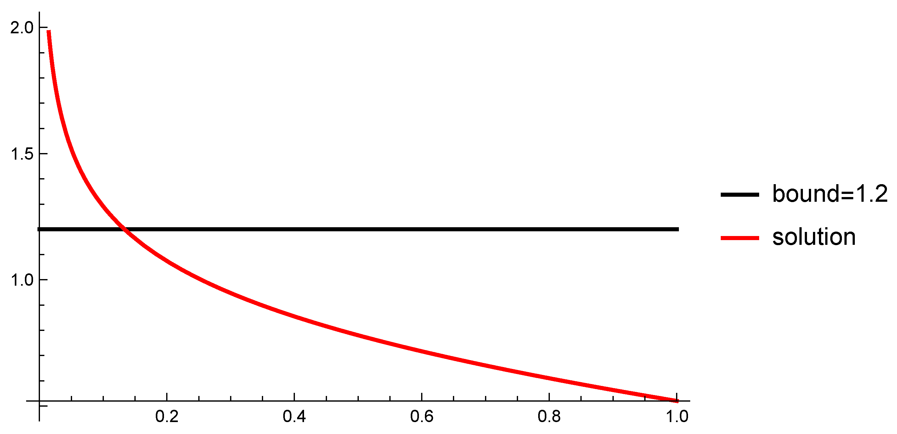
    Case 1.1. Consider D 0 0.8 , e t R L u ( t ) = 0.2 u ( t ) , f o r t > 0 . The solution is u ( t ) = ( e t 1 ) 0.2 E 0.8 , 0.8 ( 0.2 ( e t 1 ) 0.8 ) , t > 0 . It is unbounded and does not have GGLS.
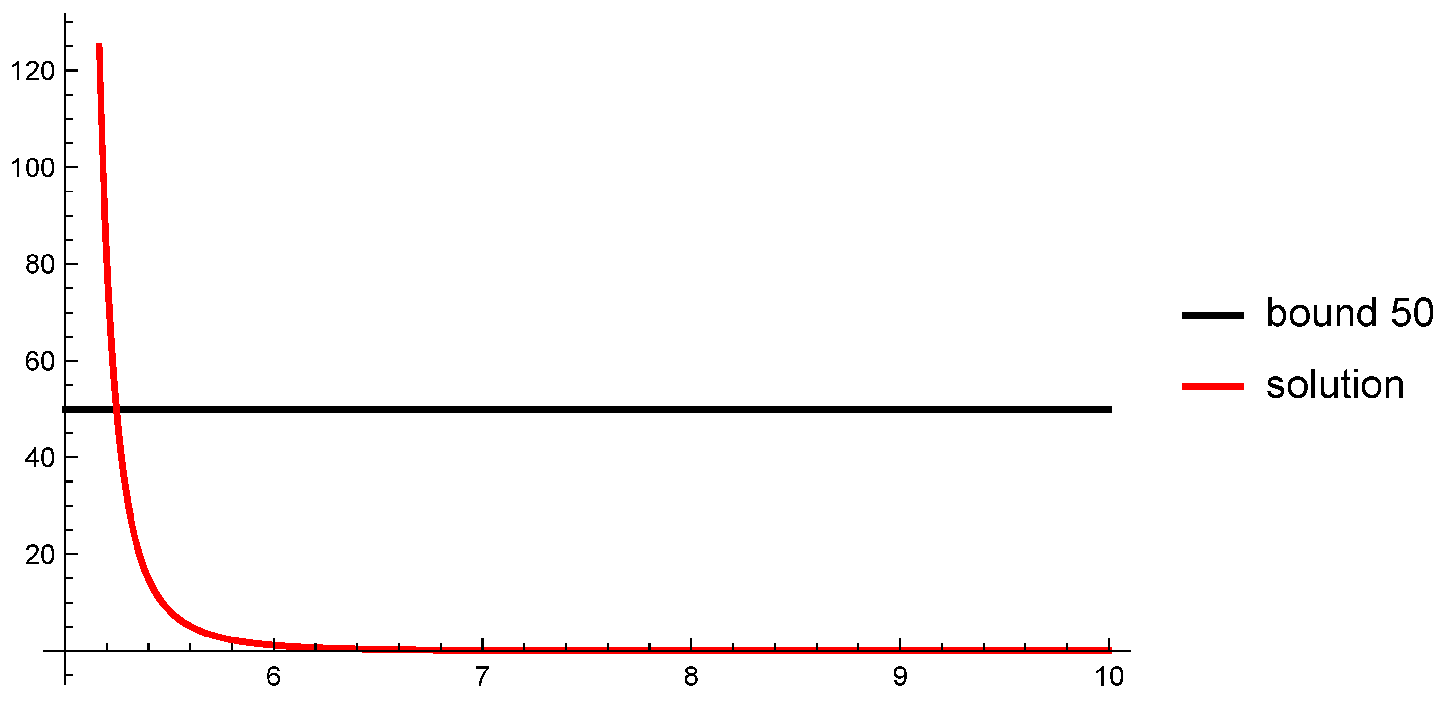
    Case 1.2. Consider LFDE D 0 0.8 , e t R L u ( t ) = 0.2 u ( t ) , f o r t > 0 . The solution is u ( t ) = ( e t 1 ) 0.2 E 0.8 , 0.8 ( 0.2 ( e t 1 ) 0.8 ) , t > 0 . It has GGLS, i.e., there exist δ = 0.133541 and T = 1.2 > 0 such that | u ( t ) | 1.2 for t > 0.133541 . The solution u ( t ) and the bound 1.2 are graphed in Figure 10, the satisfaction of the inequality and GGLS can be seen.
  • Case 2. Suppose there is a switching rule in the LFDE (31) with Θ ( t ) = e t , q = 0.8 , and u 0 = 1 .
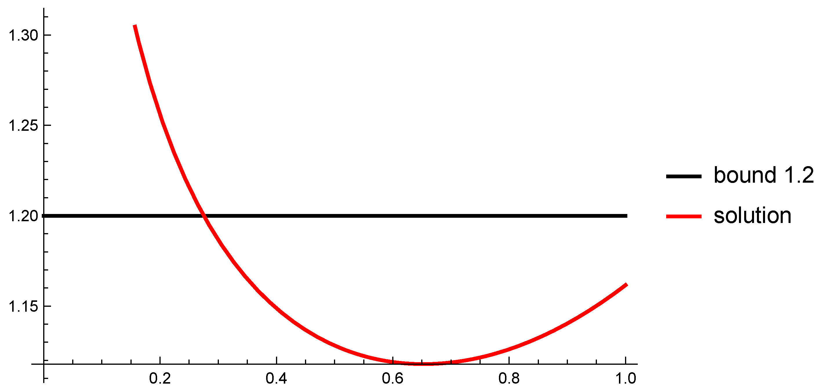
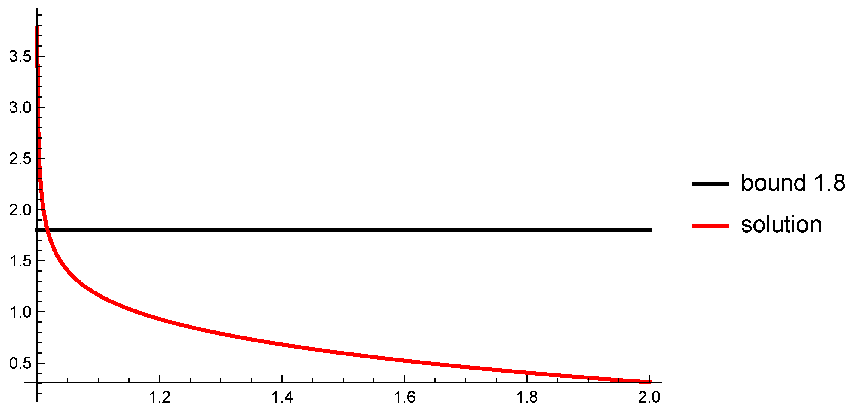
    Case 2.1. Let m = 6 < , i.e., the switching rule is activated at points 1 , 2 , 3 , 4 , and 5. In this case, condition H1 is satisfied and μ < 1 . The solution of (31) is given by (36) and graphed in Figure 5. It can be seen that there exist δ i ( 0 , ξ i + 1 ξ i ) , i = 1 , 2 , 3 , 4 , 5 , and T i > ( e i + 1 e i ) 0.2 > 0 , i = 1 , 2 , 3 , 4 , 5 , such that for the initial value u 0 = 1 , inequality (16) holds.
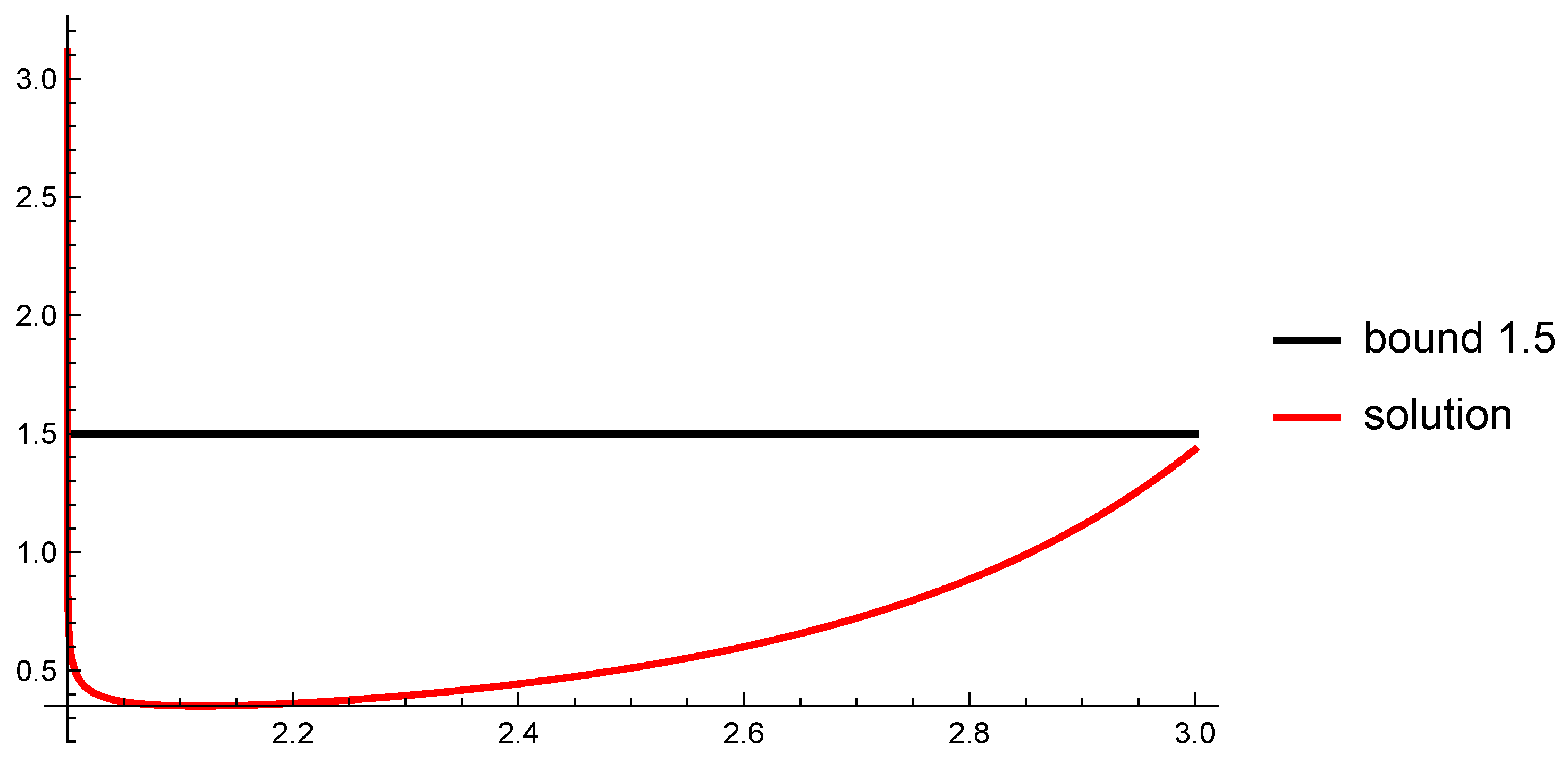
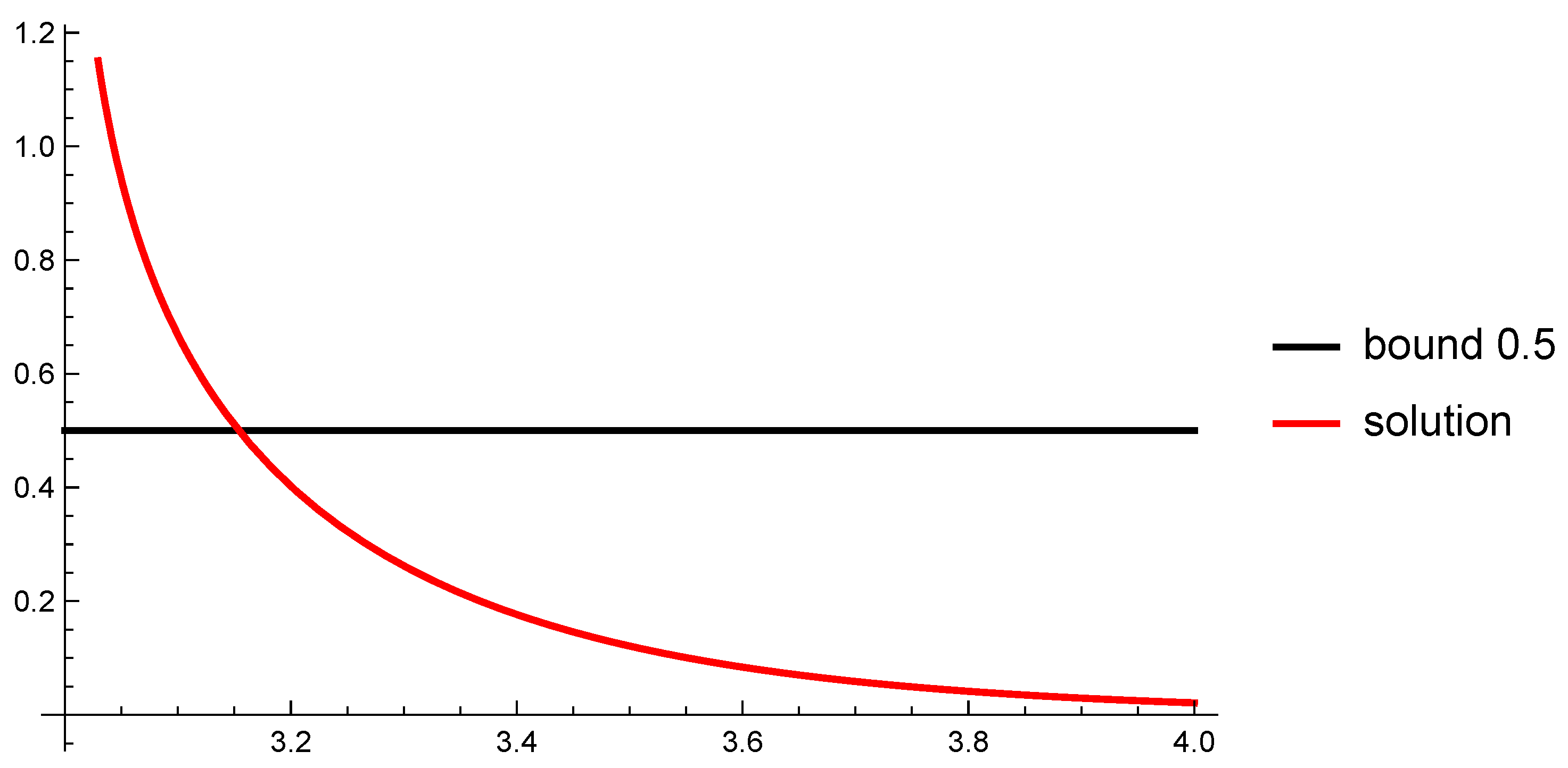
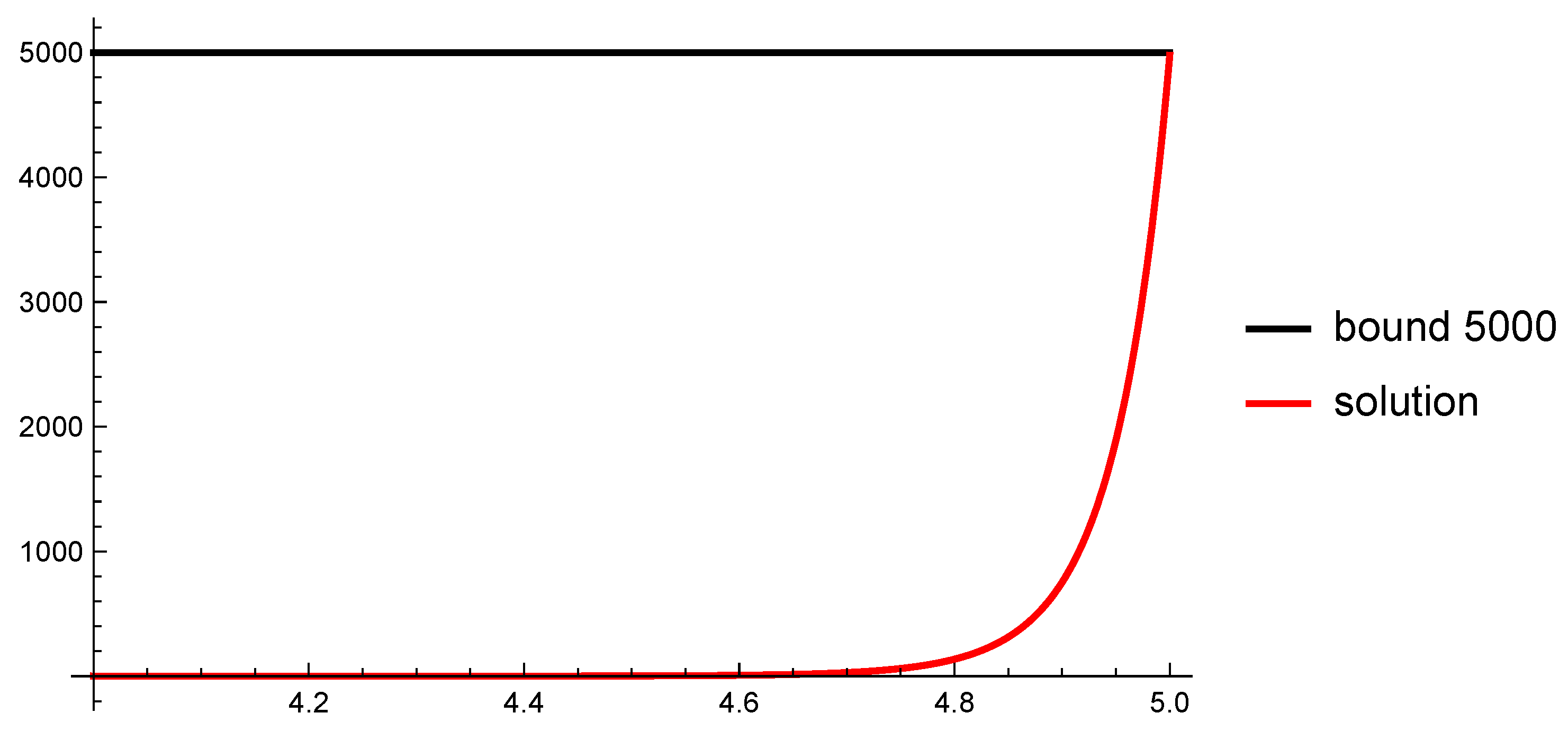
    In this case, there exist numbers δ 0 = 0.275144 ( 0 , 1 ) , T 0 = 1.2 > ( e 1 1 ) 0.2 0.89739 (see Figure 11), δ 1 = 0.01331 ( 0 , 1 ) , T 1 = 1.8 > ( e 2 e 1 ) 0.2 0.734721 (see Figure 12), δ 2 = 0.00002 ( 0 , 1 ) , T 2 = 1.5 > ( e 3 e 2 ) 0.2 0.601538 (see Figure 13), δ 3 = 0.00002 ( 0 , 1 ) , T 3 = 1.5 > ( e 4 e 3 ) 0.2 0.492498 (see Figure 14), δ 4 = 0.15403 ( 0 , 1 ) , T 4 = 0.5 > ( e 5 e 4 ) 0.2 0.403223 (see Figure 15), δ 5 = 0.000001 ( 0 , 1 ) , T 5 = 5000 > ( e 5 e 4 ) 0.2 0.330131 (see Figure 16) and δ 6 = 0.24633 ( 0 , 1 ) , T 5 = 50 > ( e 6 e 5 ) 0.2 0.330131 (see Figure 15). Therefore,
    | u ( t ) | 1.2 , t [ 0.275144 , 1 ] , | u ( t ) | 1.8 . t [ 1.01331 , 2 ] , | u ( t ) | 1.5 , t [ 2.00002 , 3 ] , | u ( t ) | 0.5 . t [ 3.15403 , 4 ] , | u ( t ) | 5000 , t [ 4.000001 , 5 ] , | u ( t ) | 50 , t > 5.24633 .
    In this case, the switched LFDE (31) has GGLS.
    Case 2.2. Let m = 4 < , i.e., the switching rule is activated at points 1 , 2 , and 3. Then the solution is not bounded and does not have GGLS.
The switching rule has a major influence on the behavior of the solution to the corresponding LFDE. For example, in spite of LFDE not being GGLS (Case 1.1), the switching rule can retain this property (Case 2.2), or it can change it (Case 2.1).

6. Discussion

In recent years, various types of switched fractional differential equations have been studied and applied for modeling; for the most part, Caputo-type derivatives have been used to describe the dynamics. Recently, for example, a Caputo fractional derivative was applied to switched systems with a piecewise constant switching rule in [18], with a variable-time switching mechanism in [15,17].
However, to our knowledge, Riemann–Liouville (R-L) fractional derivatives have not been applied in switched systems. The application of R-L fractional derivatives leads to a totally different type of switched system in two aspects. From a theoretical point of view, the application of R-L fractional derivatives requires a change in the lower limit of the fractional derivative at any switching point and a particular condition at all switching times because this fractional derivative has a singularity at the lower limit of the integral. This causes the solution of the corresponding switched system to be discontinuous at all switching times (compare with the case of Caputo fractional derivatives considered in [15,17,18]). This makes switched Riemann–Liouville fractional systems more complex than Caputo-based systems. From a practical point of view, the application of R-L fractional derivative gives us the opportunity to model adequately some anomalies at several time points in the dynamics of processes (see, for example, the neural network model in [17]).
Note that the present paper concerns switched systems with Riemann–Liouville fractional derivatives with respect to another function and generalized Lipschitz stability, whereas in [3], a Caputo–Hadamard fractional derivative is applied to an equation with delay and nonlocal conditions, and the existence and uniqueness is studied.
We consider switched fractional differential equations with RLDFs. An algorithm for obtaining their solutions is explained in detail. The application of the RLDF leads to a singularity at every switching point. This requires a special definition of global generalized Lipschitz stability in time that excludes the points of switching times. This stability is studied with Lyapunov functions, and several sufficient conditions are obtained. The provided examples illustrate the application of the obtained theoretical results and the influence of the applied function in the RLDF and the switching rule on the behavior of the solutions. They suggest possibilities regarding the application of the studied problem to models such as the Hopfield model of neural networks (see, for example, [31]), the Cohen–Grossberg model of neural networks (see, for example, [32]) and many others in which the dynamics of the units are changed at certain times. Our results are applicable for the study of stability properties of switched fractional differential equations with RLDFs.

7. Conclusions

A system of nonlinear switched fractional differential equations with an RLDF of order between zero and one is defined and studied. The main contributions of the paper can be briefly summarized as follows:
-
The lower limit of the applied RLDF changes at every switching point. This allows us to model a physical process with singularities at several time points different from the initial time.
-
A detailed algorithm for constructing the solution of the switched system with an RLDF is given. The solution of the considered switched system is discontinuous at any switching time.
-
Several examples demonstrate the influence of the applied function in the RLDF and the switching rule on the behavior of the solutions.
-
Global generalized Lipschitz stability in time is defined. This is deeply connected with the applied RLDF.
-
Several bounds on the solutions of the linear scalar switched fractional differential equations with RLDFs are obtained on intervals excluding the switching times.
-
Lyapunov functions are applied to obtain sufficient conditions on global generalized Lipschitz stability in time.
-
Cases of both finite and infinite numbers of switching times are considered.
-
We present some examples illustrating the importance of both the applied function in RLDF and the type of switching rule on the global generalized Lipschitz stability in time.

Author Contributions

Conceptualization, S.H. and D.O.; methodology, S.H. and D.O.; formal analysis, S.H. and D.O.; writing—original draft preparation, S.H. and D.O.; writing—review and editing, S.H. and D.O. All authors have read and agreed to the published version of the manuscript.

Funding

This work is partially supported by the Bulgarian National Science Fund grant number KP-06-PN62/1.

Data Availability Statement

Not applicable.

Conflicts of Interest

The authors declare no conflicts of interest.

References

  1. Kilbas, A.A.; Srivastava, H.M.; Trujillo, J.J. Theory and Applications of Fractional Differential Equations; Elsevier: North-Holland, The Netherlands, 2006. [Google Scholar]
  2. Samko, S.G.; Kilbas, A.A.; Marichev, O.I. Fractional Integrals and Derivatives: Theory and Applications; Gordon and Breach Science Publisher: London, UK, 1993. [Google Scholar]
  3. Tuan, N.H.; Tri, V.V. Existence and uniqueness of the solution to Caputo–Hadamard differential equations with delay and nonlocal conditions. Commun. Anal. Mechan. 2025, 17, 725–748. [Google Scholar]
  4. Agarwal, R.P.; Hristova, S.; O’Regan, D. Inequalities for Riemann–Liouville–type fractional derivatives of convex Lyapunov functions and applications to stability theory. Mathematics 2023, 11, 3859. [Google Scholar]
  5. Liu, S.; Wu, X.; Zhou, X.F.; Jiang, W. Asymptotical stability of Riemann–Liouville fractional nonlinear systems. Nonlinear Dyn. 2016, 86, 65–71. [Google Scholar] [CrossRef]
  6. Qin, Z.; Wu, R.; Lu, Y. Stability analysis of fractional order systems with the Riemann–Liouville derivative. Syst. Sci. Control Eng. Open Access J. 2014, 2, 727–731. [Google Scholar] [CrossRef]
  7. Bohner, M.; Hristova, S. Lipschitz stability for impulsive Riemann-Liouville fractional differential equations. Kragujev. J. Math. 2024, 48, 723–745. [Google Scholar]
  8. Agarwal, R.; Hristova, S.; O’Regan, D. Stability concepts of Riemann-Liouville fractional-order delay nonlinear systems. Mathematics 2021, 9, 435. [Google Scholar]
  9. Luchko, Y. Fractional differential equations with the general fractional derivatives of arbitrary order in the Riemann-Liouville sense. Mathematics 2022, 10, 849. [Google Scholar] [CrossRef]
  10. Stinga, P.R.; Torrea, J.L. Regularity theory and extension problem for fractional nonlocal parabolic equations and the master equation. SIAM J. Math. Anal. 2017, 49, 3893–3924. [Google Scholar] [CrossRef]
  11. Ortigueira, M.D.; Machado, J.T. On the properties of some operators under the perspective of fractional system theory. Commun. Nonl. Sci. Numer. Simul. 2020, 82, 105022. [Google Scholar] [CrossRef]
  12. Liberzon, D. Switching in Systems and Control; Birkhauser: Boston, MA, USA, 2003. [Google Scholar]
  13. Mancilla-Aguilar, J.L. A condition for the stability of switched nonlinear systems. IEEE Trans. Autom. Control 2000, 45, 20772–20779. [Google Scholar] [CrossRef]
  14. Tanwani, A.; Liberzon, D. Invertibility of nonlinear switched systems. In Proceedings of the 2008 47th IEEE Conference on Decision and Control, Cancun, Mexico, 9–11 December 2008; pp. 286–291. [Google Scholar]
  15. Zhao, Z.; Peng, Y. Qualitative theoretical research on solutions of fractional switched systems with variable-time switching mechanism. Commun. Nonlinear Sci. Numer. Simul. 2025, 143, 108645. [Google Scholar] [CrossRef]
  16. Sierociuk, D.; Macias, M.; Malesza, W. Analog modeling of fractional switched-order derivatives: Experimental approach. In Advances in the Theory and Applications of Non-integer Order Systems; Mitkowski, W., Kacprzyk, J., Baranowski, J., Eds.; Lecture Notes in Electrical Engineering; Springer: Heidelberg, Germany, 2013; Volume 257, pp. 271–280. [Google Scholar]
  17. Cao, B.; Nie, X.; Zheng, W.X.; Cao, J. Multistability of state-dependent switched fractional-order Hopfield neural networks with Mexican-hat activation function and its application in associative memories. IEEE Trans. Neural Netw. Learn. Syst. 2025, 36, 1213–1227. [Google Scholar] [PubMed]
  18. Agarwal, R.P.; Hristova, S.; O’Regan, D. Stability of nonlinear switched fractional differential equations with short memory. Fractal Fract. 2025, 9, 598. [Google Scholar] [CrossRef]
  19. Gallegos, J.A.; Aguila-Camacho, N.; Duarte-Mermoud, M.A.; Travieso-Torres, J.C.; Ceballos-Benavides, G.E. Switched systems with changing derivation order: Stability and applications. J. Frankl. Inst. 2021, 358, 3943–3963. [Google Scholar] [CrossRef]
  20. Wang, J.R.; Fečkan, M.; Zhou, Y. Fractional order differential switched systems with coupled nonlocal initial and impulsive conditions. Bull. Sci. Math. 2017, 141, 727–746. [Google Scholar] [CrossRef]
  21. Feng, T.; Wang, L.; Chen, Y. Finite-time stability of fractional-order switched systems based on Lyapunov method. Fractal Fract. 2025, 9, 94. [Google Scholar]
  22. Wang, J.R.; Ibrahim, A.G.; O’Regan, D. Hilfer-type fractional differential switched inclusions with noninstantaneous impulsive and nonlocal conditions. Nonlinear Anal. Model. Control 2018, 23, 921–941. [Google Scholar] [CrossRef]
  23. Kumar, V.; Malik, M.; Baleanu, D. Results on Hilfer fractional switched dynamics system with non-instantaneous impulses. Pramana—J. Phys. 2022, 96, 172. [Google Scholar] [CrossRef]
  24. Durgaa, N.; Nageshwari, S.; Chalishajar, D.N. Total controllability of stochastic non-instantaneous impulsive Hilfer fractional switched dynamic systems with deviated arguments. Stoch. Anal. Appl. 2025, 43, 273–302. [Google Scholar] [CrossRef]
  25. Fahad, H.M.; Fernandez, A. Operational calculus for the Riemann-Liouville fractional derivative with respect to a function and its applications. Fract. Calc. Appl. Anal. 2021, 24, 518–540. [Google Scholar]
  26. Nieto, J.J.; Alghnmi, M.; Ahmad, B.; Alsaedi, A.; Alharbi, B. On fractional integrals and derivatives of a functions with respect to another function. Fractals 2023, 31, 2340066. [Google Scholar] [CrossRef]
  27. Jiang, D.; Bai, C. Existence results for coupled implicit Θ-Riemann-Liouville fractional differential equations with nonlocal conditions. Axioms 2022, 11, 103. [Google Scholar]
  28. Hristova, S.; Tersian, S.; Terzieva, R. Lipschitz stability in time for Riemann-Liouville fractional differential equations. Fractal Fract. 2021, 5, 37. [Google Scholar]
  29. Devi, J.V.; Mc Rae, F.A.; Drici, Z. Variational Lyapunov method for fractional differential equations. Comput. Math. Appl. 2012, 64, 2982–2989. [Google Scholar] [CrossRef]
  30. Othmane, I.B.; Nisse, L.; Abdeljawad, T. On Cauchy-type problems with weighted R-L fractional derivatives of a function with respect to another function and comparison theorems. AIMS Math. 2024, 9, 14106–14129. [Google Scholar] [CrossRef]
  31. Wu, X.; Liu, S.; Wang, Y. Stability analysis of Riemann-Liouville fractional-order neural networks with reaction-diffusion terms and mixed time-varying delays. Neurocomputing 2021, 431, 169–178. [Google Scholar]
  32. Li, Z.; Jiang, W.; Zhang, Y. Dynamic analysis of fractional-order neural networks with inertia. AIMS Math. 2022, 7, 16889–16906. [Google Scholar] [CrossRef]
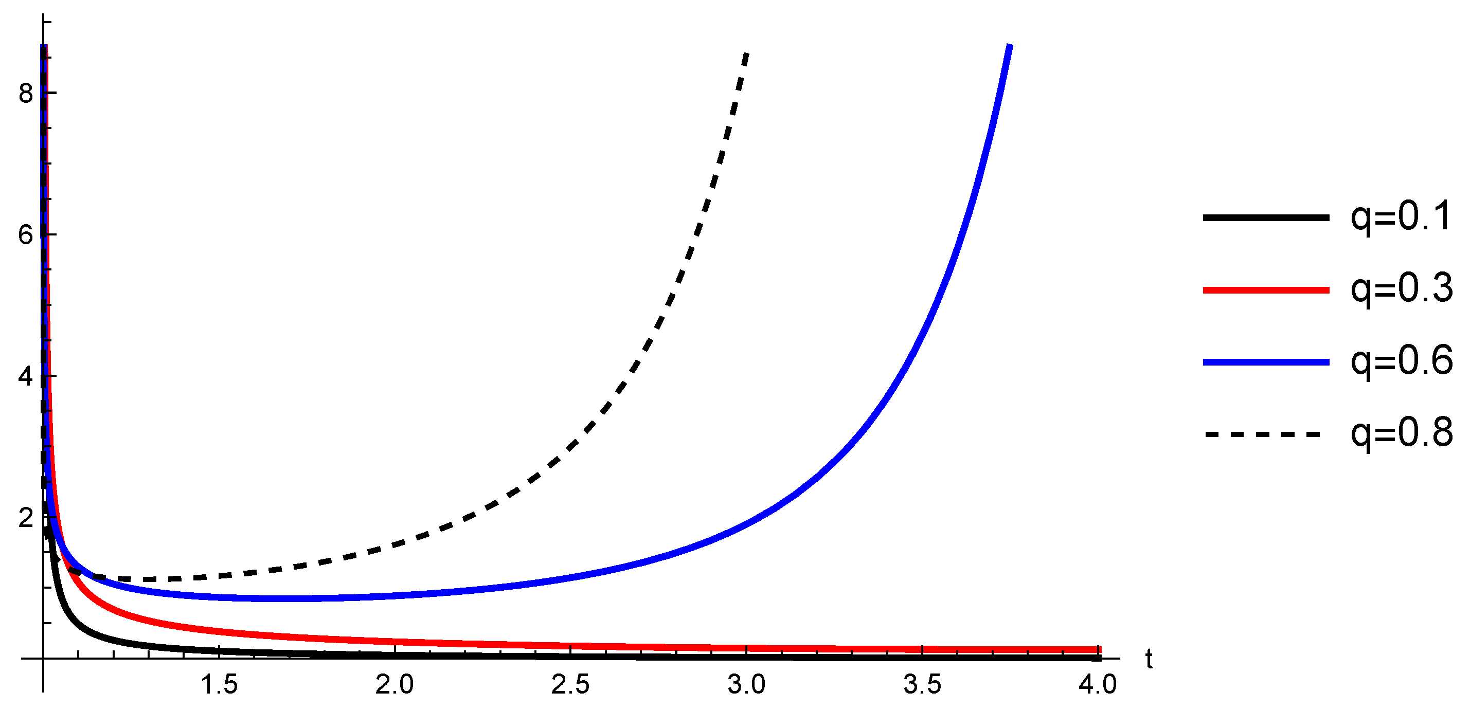
Figure 1. Graph of the function h ( t ) with Θ ( t ) = e t , A = 0.2 .
Fractalfract 10 00450 g001
Figure 2. Graph of the function h ( t ) with Θ ( t ) = e t , A = 1 .
Fractalfract 10 00450 g002
Figure 3. Graph of the function h ( t ) with Θ ( t ) = t t + 1 , A = 0.2 .
Fractalfract 10 00450 g003
Figure 4. Graph of the function h ( t ) with Θ ( t ) = t t + 1 , A = 1 .
Fractalfract 10 00450 g004
Figure 5. Graph of the solution of (31) with Θ ( t ) = e t .
Fractalfract 10 00450 g005
Figure 6. Graph of the solution of (31) with Θ ( t ) = t t + 1 .
Fractalfract 10 00450 g006
Figure 7. Graph of the solution of (38) with Θ ( t ) = e t .
Fractalfract 10 00450 g007
Figure 8. Graph of the solution of (38) with Θ ( t ) = t t + 1 .
Fractalfract 10 00450 g008
Figure 9. Graph of the solution of (38) with the classical RL fractional derivative, i.e., Θ ( t ) t .
Fractalfract 10 00450 g009
Figure 10. Graph of the solution in Case 1.2.
Fractalfract 10 00450 g010
Figure 11. Graph of the solution in Case 2.1 on the interval ( 0 , 1 ) .
Fractalfract 10 00450 g011
Figure 12. Graph of the solution in Case 2.1 on the interval ( 1 , 2 ) .
Fractalfract 10 00450 g012
Figure 13. Graph of the solution in Case 2.1 on the interval ( 2 , 3 ) .
Fractalfract 10 00450 g013
Figure 14. Graph of the solution in Case 2.1 on the interval ( 3 , 4 ) .
Fractalfract 10 00450 g014
Figure 15. Graph of the solution in Case 2.1 on the interval ( 4 , 5 ) .
Fractalfract 10 00450 g015
Figure 16. Graph of the solution in Case 2.1 on the interval ( 5 , ) .
Fractalfract 10 00450 g016
Disclaimer/Publisher’s Note: The statements, opinions and data contained in all publications are solely those of the individual author(s) and contributor(s) and not of MDPI and/or the editor(s). MDPI and/or the editor(s) disclaim responsibility for any injury to people or property resulting from any ideas, methods, instructions or products referred to in the content.