A Parallel Krylov Subspace Iterative Scheme for Variable-Order Fractional Advection–Diffusion–Reaction Equation

Abstract

This paper is concerned with the numerical solution of the variable-order time fractional advection–diffusion–reaction equation (VO-TFADRE) in two space dimensions. We first propose a Crank–Nicolson (C-N) discretization scheme based on central difference operators and L1 formula for space and time variables, respectively. Then, we apply the C-N scheme to construct a new algorithm, namely the explicit group (EG) method, for the model problem under consideration. The EG method utilizes the idea of small fixed-size groups of mesh points and comes with computational merits as compared with the C-N scheme. Stability and convergence analyses are given in this work. The resulting discretization leads to large sparse linear systems, which are solved using the Bi-CGSTAB iterative method. Numerical experiments demonstrate that both the C–N and EG schemes achieve accurate approximations, while the EG method significantly reduces computational time. To economize further on the computational cost, we propose a parallelized version of the EG method for solving the VO-TFADRE. Carried out numerical simulations reveal that the parallel algorithm is more efficient than the serial algorithm for solving the problem under consideration.

1. Introduction

Over the last few decades, fractional calculus has gained tremendous interest from scholars and practitioners, making it one of the hot areas of applied mathematics [1,2]. Fractional calculus generalizes classical calculus and extends the order of differential and integral operators to an arbitrary order. The spectrum of applications of fractional calculus is wide and includes, but is not limited to, physics, control problems, artificial neural networks, signal and image processing, epidemic models, mechanics and dynamic systems, economic processes, materials, and computer vision [3,4,5]. One of the processes that has been widely investigated with the help of fractional calculus is the anomalous diffusion phenomenon. This refers to the situation where the mean square displacement is no longer linear in time. Fractional diffusion equations have served as important mathematical models for describing such phenomena. Consequently, a plethora of numerical methods have been developed for solving these equations, such as finite difference methods [6], finite element methods [7], meshless methods [8], collocation methods [9], and others. Recently, researchers have made modifications to the standard anomalous diffusion processes by incorporating noise terms and particle diffusion in a parabolic potential [10,11].

Variable-order time fractional partial differential equations (VO-TFPDEs) are one of the most important tools of fractional calculus for modeling various real-life phenomena with variable memory properties [12,13]. At the same time, the analytical solution of VO-TFPDEs is not an easy task. In fact, it is extremely difficult to solve VO-TFPDEs analytically, and in many cases, analytical solutions cannot be found due to the extra complexity of dealing with the VO fractional derivative. Consequently, many researchers have paid attention to solving VO-TFPDEs numerically. From the literature, one can easily note that most existing numerical methods rely on the finite difference method (FDM). It should be mentioned that, while FDMs are widely used for solving various types of FPDEs, the conditional stability of explicit finite difference techniques and the necessity for significant CPU time in implicit finite difference schemes limit their usefulness. Hence, the development of stable, efficient, and accurate numerical schemes for dealing with VO-TFPDEs is of great importance. Diethelm et al. [14] have specified the goal of developing efficient numerical algorithms that diminish the computational challenges of solving fractional differential equations as one of the main issues for further research in the field of fractional calculus. In this line of thought, the main aim of this article is to construct an efficient numerical algorithm that accounts for the solution of a subclass of VO-TFPDEs, that is, the VO time fractional advection–diffusion–reaction equation (VO-TFADRE) of the following form:

$$\{\begin{array}{l}{}_0{}^{C}D_t^{\alpha (x,y,t)}s(x,y,t)+s_x+s_y-s_{xx}-s_{yy}+s=g(x,y,t),(x,y,t)\in \Omega \times (0,T],\\ s(x,y,t)=p(x,y,t),(x,y,t)\in \mathsf{\partial }\Omega \times (0,T],\\ s=q(x,y),(x,y,t)\in \overline{\Omega }\times \{0\},\end{array}$$

(1)

where $\Omega =(0,K)\times (0,K)$ is a bounded domain and $\mathsf{\partial }\Omega$ is its boundary, $\overline{\Omega }=\Omega \cup \mathsf{\partial }\Omega$, T and K are positive constants, $g(x,y,t)$ is the source term function, and $p(x,y,t)$ and $q(x,y)$ are known smooth functions. The current study deals with a domain of regular geometry; however, works that consider fractional problems associated with complex geometries can also be found in the literature [15,16]. Here, the finite element method emerges as an effective technique for solving these problems [17]. For a comprehensive treatment of numerical methods for fractional differential equations, we also refer to [18].

The VO Caputo-type fractional derivative ${}_0{}^{C}D_t^{\alpha (x,y,t)}s(x,y,t)$ of order $0<\alpha (x,y,t)\le 1$, $\alpha (x,y,t)\in C(\overline{\Omega }\times [0,T])$ with respect to time t is defined as

$${}_0{}^{C}D_t^{\alpha (x,y,t)}s(x,y,t)=\left\{\begin{array}{c}{\displaystyle \frac{1}{\Gamma (1-\alpha (x,y,t\left)\right)}}{\int }_0^t{(t-\xi )}^{-\alpha (x,y,t)}{\displaystyle \frac{\mathsf{\partial }s(x,y,\xi )}{\mathsf{\partial }\xi }}d\xi ,0<\alpha (x,y,t)<1,\hfill \\ {\displaystyle \frac{\mathsf{\partial }s(x,y,t)}{\mathsf{\partial }t}},\alpha (x,y,t)=1.\hfill \end{array}\right.$$

This definition clearly indicates that the VO Caputo derivative is history dependent, such that the fractional derivative at time t depends on the entire history of the solution. Recent studies highlighting the importance of the memory effect can be found in [19,20].

For convenience of theoretical analysis, we assume the existence of a solution $s(x,y,t)\in C^{4,4,2}(\overline{\Omega }\times [0,T])$, where $C^{i,j,k}$ is the class of functions, continuous together with their partial derivatives of the order i with respect to x, order j with respect to y, and order k with respect to t on $\overline{\Omega }\times [0,T]$.

In recent years, fractional differential operators of fixed order, also known as constant-order (CO) fractional derivatives, have achieved remarkable success in modeling a wide range of real-world phenomena. A main reason for the popularity of CO fractional derivatives is their memory and nonlocal properties, which make them suitable for describing diverse complex physical systems. Although CO fractional derivatives are pivotal for modeling numerous important physical problems, they cannot address significant classes of physical phenomena where the order itself is changing with respect to dependent and/or independent variables. The last case leads to the so-called VO fractional derivatives, where the order is a function of certain variables. For instance, it has been discovered that the reaction kinetics of proteins display relaxation mechanisms that are accurately characterized by a fractional order depending on the temperature [21]. Accordingly, many FPDEs have been extended from the CO case to the VO case for better capture of the properties of complex physical systems. The list of examples includes the fractional diffusion equation, fractional cable equation, fractional advection–diffusion equation, fractional Burgers’ equation, fractional mobile/immobile equation, fractional Black–Scholes equation, fractional Schrodinger equation, and others.

The TFADRE is an important mathematical model for describing several phenomena, especially those involving the coupling of a reaction term with diffusion and advection processes such as biological and environmental systems, chemical engineering problems, oil reservoir simulations, and the transport of mass and energy. In these phenomena, the unknown solution may represent chemical species, concentration, population size, or other certain quantities. Therefore, it is worthwhile to study the numerical solution of the VO-TFADRE.

During the last decade, many research papers have been devoted to the numerical treatment of the CO-TFADRE. For instance, finite difference schemes [22,23,24,25,26], finite element methods [27,28,29], spectral methods [30,31], and meshless methods [32] have been successfully developed for solving the CO-TFADRE. On the other hand, few studies have been directed toward solving the VO-TFADRE numerically. For instance, Li and Wu [33] proposed a reproducing-kernel-functions-based meshless method for solving the VO-TFADRE. In their methodology, the authors combined the Mittag–Leffler kernel function and the Gaussian kernel function to establish a new binary reproducing kernel function. Then, they employed a space-time collocation technique to construct the meshless method. Chen et al. [34] combined shifted Gegenbauer polynomials along with a spectral collocation technique to solve the VO-TFADRE involving a time fractional derivative in the Atangana–Baleanu–Caputo sense. Hosseininia et al. [35] introduced a hybrid method based on the orthogonal Bernoulli polynomials and radial basis functions under the framework of Heydari–Hosseininia VO fractional derivative. Kheirkhah et al. [36] presented an accurate numerical scheme for solving one-dimensional and two-dimensional VO-TFADRE. The suggested discrete scheme is based on a third-order weighted-shifted Grünwald formula in time and a fourth-order compact finite difference operator in space. The authors also discussed the stability and convergence of their compact scheme. Xu et al. [37] developed a meshless method based on radial basis functions for simulating the VO-TFADRE. Several numerical experiments were provided to confirm the efficiency and applicability of the proposed method. More recently, Liu et al. [38] proposed a high-order compact difference scheme along with its theoretical analysis for the one-dimensional VO-TFADRE. One can note that significant effort has been invested in solving the CO-TFADRE, while few works have been devoted to handling the VO-TFADRE. A reason for this is the extra complexity of dealing with VO differential operators. For example, numerical treatment of these operators necessitate the dynamic update of discretization weights, which may complicate the theoretical analysis further. In this line of thought, and motivated with the applications of TFADRE with variable exponent [39], we present the current study.

Over the last few years, interest in developing explicit group methods for solving various types of CO-TFPDEs has become increasingly evident. Equations including the fractional cable equation [40], the fractional diffusion equation [41,42], the fractional Burgers’ equation [43,44], the fractional advection–diffusion equation [45], the fractional telegraph equation [46], the fractional reaction–diffusion equation [47], and the fractional Rayleigh–Stokes equation [48] have been solved using explicit group methods. The construction of these methods is based on arranging the grid points of the solution domain into small, fixed-size groups of points, which results in numerical schemes with better computational merits compared to point-wise numerical techniques. Other advantages such as simplicity, ease of programming, and applicability for parallel implementation made explicit group methods an attractive option for simulating several CO fractional models. To the best of our knowledge, the development of explicit group methods for VO-TFPDEs is scarce in the literature [12]. The extension and analysis of these methods for VO fractional models is more challenging due to the variable exponent in the kernel of the VO fractional derivative. Consequently, the analysis and application of explicit group methods for solving VO-TFPDEs is far from complete.

In this paper, we will construct an explicit group (EG) method based on a point-wise Crank–Nicolson (C-N) difference scheme for solving the VO-TFADRE in two space dimensions. In addition, the theoretical aspects of stability and convergence will be discussed via a Fourier analysis approach. A comparative study between the EG method and the C-N scheme will be performed in light of numerical experiments. To enhance the computational efficiency further, parallel implementation of the EG method will also be considered in the present work. In summary, the focus of this paper is on the following items:

• Detailed derivation of the C-N difference scheme and construction of the EG method to solve the VO-TFADRE with suitable initial and boundary conditions.
• Fourier-type stability analysis and convergence properties of the proposed method.
• Parallel implementation of the EG method to improve the computational efficiency further.

The remaining content of this paper is outlined as follows. In the next section, we present the derivation of the C-N difference scheme and, on its basis, the construction of the EG method for solving the VO-TFADRE (1). In Section 3, we investigate the stability and convergence of the proposed method. Several numerical simulations supported by graphical and tabular data are given in Section 4. The parallel implementation of the EG method to enhance the performance is discussed in Section 5. Finally, the paper is concluded concisely in Section 6.

2. The Proposed EG Method for VO-TFADRE

2.1. The C-N Discretization of the VO-TFADRE

In this part, we discretize the model problem (1). To this end, choose $M_x,M_y,$ and N, which denote, respectively, the number of partitions in the x, y, and t directions. Let $h_x=K/M_x$ and $h_y=K/M_y$ be the spatial step sizes in the x and y directions, respectively, and define the discrete spatial grid ${\Omega }_h=\left\{(x_i,y_j)\right|x_i=i{h}_x,y_j=j{h}_y,i=0,1,\dots ,M_x,j=0,1,\dots ,M_y\}$. Let $\tau =T/N$ be the temporal step size and define the discrete temporal grid ${\Omega }_{\tau }=\{t_k=k\tau ,k=0,1,\dots ,N\}$. Let $t_{k+1/2}={\displaystyle \frac{t_k+t_{k+1}}{2}}$, $s_{i,j}^k$ and $S_{i,j}^k$ be the exact and the numerical solutions at the grid point $(x_i,y_j,t_k)$, respectively.

Now, we discretize the model problem (1) at the grid point $(x_i,y_j,t_{k+1/2})$, $i=1,2,\dots ,M_x-1$, $j=1,2,\dots ,M_y-1$, $k=0,1,\dots ,N-1$. The first-order spatial derivatives are discretized by the central difference quotient,

$$\begin{array}{cc}\hfill s_x(x_i,y_j,t_{k+1/2})& ={\displaystyle \frac{1}{2}}\left({\delta }_x{s}_{i,j}^k+{\delta }_x{s}_{i,j}^{k+1}\right)+O({\tau }^2+h_x^2+h_y^2),\hfill \\ \hfill s_y(x_i,y_j,t_{k+1/2})& ={\displaystyle \frac{1}{2}}\left({\delta }_y{s}_{i,j}^k+{\delta }_y{s}_{i,j}^{k+1}\right)+O({\tau }^2+h_x^2+h_y^2),\hfill \end{array}$$

(2)

where

$$\begin{array}{c}\hfill {\delta }_x{s}_{i,j}^k={\displaystyle \frac{s_{i+1,j}^k-s_{i-1,j}^k}{2h_x}},{\delta }_y{s}_{i,j}^k={\displaystyle \frac{s_{i,j+1}^k-s_{i,j-1}^k}{2h_y}}.\end{array}$$

(3)

Using the central difference quotient to discretize the second-order spatial derivatives, we obtain

$$\begin{array}{cc}\hfill s_{xx}(x_i,y_j,t_{k+1/2})& ={\displaystyle \frac{1}{2}}\left({\delta }_x^2{s}_{i,j}^k+{\delta }_x^2{s}_{i,j}^{k+1}\right)+O({\tau }^2+h_x^2+h_y^2),\hfill \\ \hfill s_{yy}(x_i,y_j,t_{k+1/2})& ={\displaystyle \frac{1}{2}}\left({\delta }_y^2{s}_{i,j}^k+{\delta }_y^2{s}_{i,j}^{k+1}\right)+O({\tau }^2+h_x^2+h_y^2),\hfill \end{array}$$

(4)

where

$$\begin{array}{c}\hfill {\delta }_x^2{s}_{i,j}^k={\displaystyle \frac{s_{i+1,j}^k-2s_{i,j}^k+s_{i-1,j}^k}{h_x^2}},{\delta }_y^2{s}_{i,j}^k={\displaystyle \frac{s_{i,j+1}^k-2s_{i,j}^k+s_{i,j-1}^k}{h_y^2}}.\end{array}$$

(5)

To approximate the VO fractional derivative ${}_0{}^{C}D_t^{\alpha (x,y,t)}s$ at $(x_i,y_j,t_{k+1/2})$, we partition the interval $[0,t_{k+1/2}]$ uniformly and use linear interpolation on each sub-interval, which produces the following L1 formula:

$$\begin{array}{cc}\hfill & {}_0{}^{C}D_t^{{\alpha }^{i,j,k+1/2}}s(x_i,y_j,t_{k+1/2})\hfill \\ \hfill & ={\sigma }^{i,j,k}\left[{\mathcal{Z}}_1^{i,j,k}{s}_{i,j}^k-{\displaystyle \sum _{m=1}^{k-1}}\left({\mathcal{Z}}_{k-m}^{i,j,k}-{\mathcal{Z}}_{k-m+1}^{i,j,k}\right)s_{i,j}^m-{\mathcal{Z}}_k^{i,j,k}{s}_{i,j}^0+{\displaystyle \frac{s_{i,j}^{k+1}-s_{i,j}^k}{2^{1-{\alpha }^{i,j,k+1/2}}}}\right]\hfill \\ \hfill & +O\left(\tau \right),\hfill \end{array}$$

(6)

where ${\alpha }^{i,j,k+1/2}=\alpha (x_i,y_j,t_{k+1/2})$, and

$$\begin{array}{cc}\hfill {\sigma }^{i,j,k}=& {\displaystyle \frac{1}{\Gamma (2-{\alpha }^{i,j,k+1/2}){\tau }^{{\alpha }^{i,j,k+1/2}}}},\hfill \\ \hfill {\mathcal{Z}}_m^{i,j,k}=& {(m+1/2)}^{1-{\alpha }^{i,j,k+1/2}}-{(m-1/2)}^{1-{\alpha }^{i,j,k+1/2}}.\hfill \end{array}$$

A complete derivation of the formula in (6) along with its corresponding weights can be found in [49]. The substitution of Equations (2), (4), and (6) into the model problem (1) leads to the discretization of the VO-TFADRE at the point $(x_i,y_j,t_{k+1/2})$,

$$\begin{array}{cc}\hfill & {\sigma }^{i,j,k}\left[{\mathcal{Z}}_1^{i,j,k}{s}_{i,j}^k-{\displaystyle \sum _{m=1}^{k-1}}\left({\mathcal{Z}}_{k-m}^{i,j,k}-{\mathcal{Z}}_{k-m+1}^{i,j,k}\right)s_{i,j}^m-{\mathcal{Z}}_k^{i,j,k}{s}_{i,j}^0+{\displaystyle \frac{s_{i,j}^{k+1}-s_{i,j}^k}{2^{1-{\alpha }^{i,j,k+1/2}}}}\right]\hfill \\ \hfill & +{\displaystyle \frac{1}{2}}\left({\delta }_x{s}_{i,j}^k+{\delta }_x{s}_{i,j}^{k+1}\right)+{\displaystyle \frac{1}{2}}\left({\delta }_y{s}_{i,j}^k+{\delta }_y{s}_{i,j}^{k+1}\right)-{\displaystyle \frac{1}{2}}\left({\delta }_x^2{s}_{i,j}^k+{\delta }_x^2{s}_{i,j}^{k+1}\right)\hfill \\ \hfill & -{\displaystyle \frac{1}{2}}\left({\delta }_y^2{s}_{i,j}^k+{\delta }_y^2{s}_{i,j}^{k+1}\right)+{\displaystyle \frac{s_{i,j}^{k+1}+s_{i,j}^k}{2}}=g_{i,j}^{k+1/2}+O(\tau +h_x^2+h_y^2).\hfill \end{array}$$

(7)

Upon the substitutions of Equations (3) and (5) into Equation (7), omitting the truncation error, and replacement of $s_{i,j}^k$ with its numerical approximation $S_{i,j}^k$, the following C-N difference scheme for VO-TFADE (1) is obtained:

$$\begin{array}{cc}\hfill & J_{i,j}^k{S}_{i,j}^{k+1}=\left(P_1^{i,j,k}-Q_1^{i,j,k}\right)(S_{i+1,j}^{k+1}+S_{i+1,j}^k)\hfill \\ \hfill & +\left(P_1^{i,j,k}+Q_1^{i,j,k}\right)(S_{i-1,j}^{k+1}+S_{i-1,j}^k)+\left(P_2^{i,j,k}-Q_2^{i,j,k}\right)(S_{i,j+1}^{k+1}+S_{i,j+1}^k)\hfill \\ \hfill & +\left(P_2^{i,j,k}+Q_2^{i,j,k}\right)(S_{i,j-1}^{k+1}+S_{i,j-1}^k)+H_{i,j}^k{S}_{i,j}^k\hfill \\ \hfill & +{\displaystyle \sum _{m=1}^{k-1}}\left({\mathcal{Z}}_{k-m}^{i,j,k}-{\mathcal{Z}}_{k-m+1}^{i,j,k}\right)S_{i,j}^m+{\mathcal{Z}}_k^{i,j,k}{S}_{i,j}^0+{\gamma }^{i,j,k}{g}_{i,j}^{k+1/2},\hfill \\ \hfill & i=1,2,\dots ,M_x-1,j=1,2,\dots ,M_y-1,k=0,1,\dots ,N-1,\hfill \end{array}$$

(8)

with the discrete initial and boundary conditions

$$\begin{array}{cc}\hfill S_{i,j}^0& =q(i{h}_x,j{h}_y),i=0,1,\dots ,M_x,j=0,1,\dots ,M_y,\hfill \\ \hfill S_{0,j}^k& =p_1(j{h}_y,k\tau ),S_{M_x,j}=p_2(j{h}_y,k\tau ),j=0,1,\dots ,M_y,k=1,2,\dots ,N,\hfill \\ \hfill S_{i,0}^k& =p_3(i{h}_x,k\tau ),S_{i,M_y}=p_4(i{h}_x,k\tau ),i=0,1,\dots ,M_x,k=1,2,\dots ,N,\hfill \end{array}$$

(9)

where

$$\begin{array}{cc}\hfill & J_{i,j}^k=\left(0.5^{1-{\alpha }^{i,j,k+1/2}}+0.5{\gamma }^{i,j,k}+2P_1^{i,j,k}+2P_2^{i,j,k}\right),\hfill \\ & H_{i,j}^k=\left(0.5^{1-{\alpha }^{i,j,k+1/2}}-0.5{\gamma }^{i,j,k}-{\mathcal{Z}}_1^{i,j,k}-2P_1^{i,j,k}-2P_2^{i,j,k}\right),\hfill \\ \hfill & {\gamma }^{i,j,k}={\tau }^{{\alpha }^{i,j,k+1/2}}\Gamma (2-{\alpha }^{i,j,k+1/2}),P_1^{i,j,k}={\displaystyle \frac{{\gamma }^{i,j,k}}{2h_x^2}},P_2^{i,j,k}={\displaystyle \frac{{\gamma }^{i,j,k}}{2h_y^2}},\hfill \\ \hfill & Q_1^{i,j,k}={\displaystyle \frac{{\gamma }^{i,j,k}}{4h_x}},Q_2^{i,j,k}={\displaystyle \frac{{\gamma }^{i,j,k}}{4h_y}}.\hfill \end{array}$$

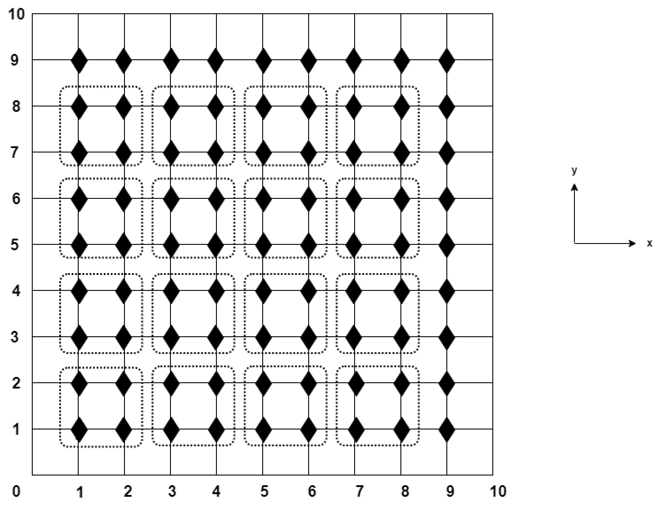
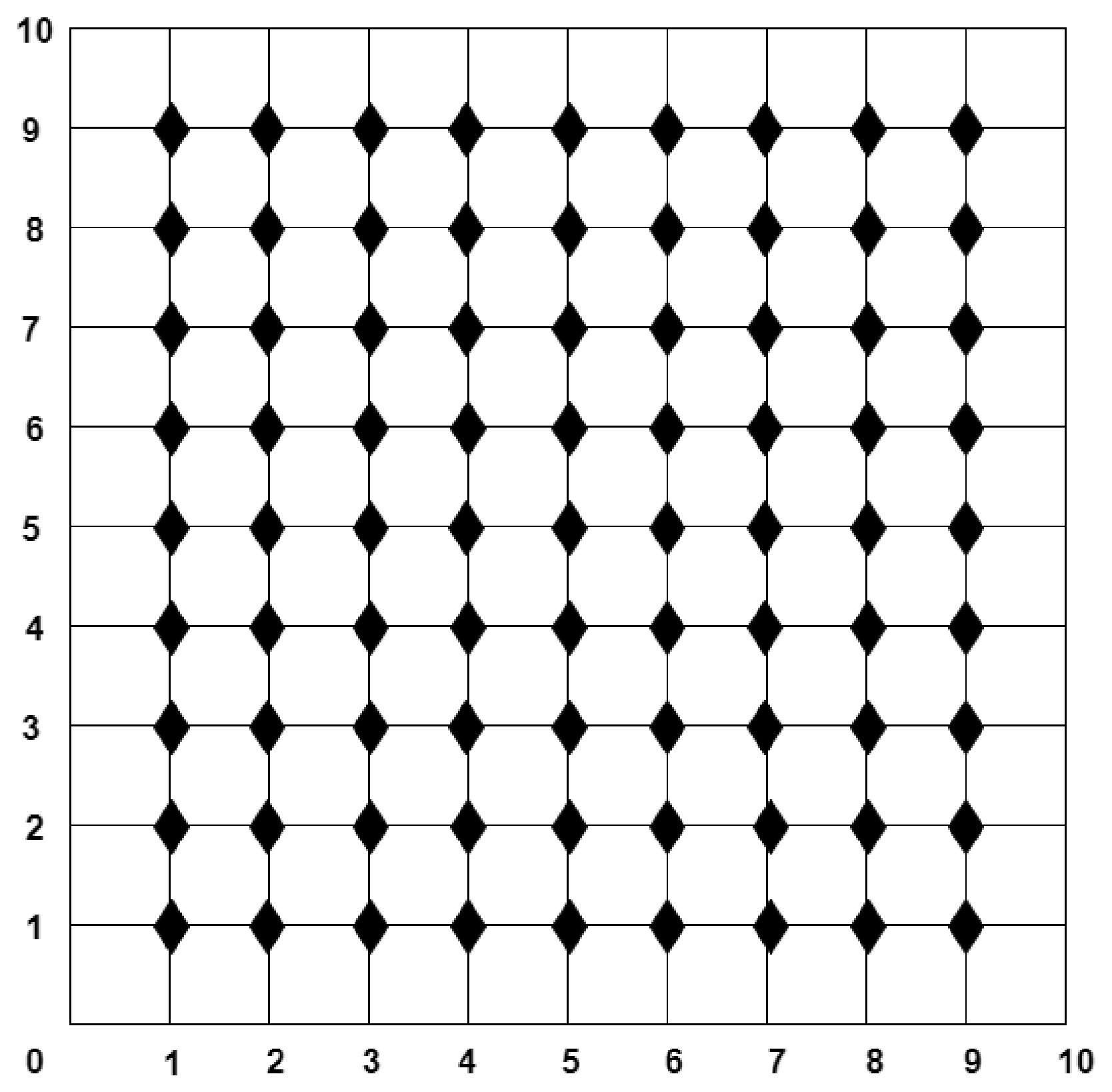
The C-N difference scheme (8) is a point-wise numerical scheme for solving the VO-TFADRE (1). This means that at each time level k, the solution values at each grid point ⧫ shown in Figure 1 are computed using Equation (8) until a certain predefined convergence criterion is met. The obtained solutions are then used as an initial guess for the next time level $k+1$. Such a process continues until the targeted time level is reached. Due to the non-local property of the temporal fractional derivative, the described solution algorithm may lead to prohibitively expensive simulations in terms of computational cost. To surmount such a challenge, we propose the EG method in the next subsection.

2.2. The Construction of the EG Method for the VO-TFADRE

The goal of this subsection is to develop an efficient and accurate numerical scheme, the EG method, for solving the VO-TFADRE (1). To this end, we use the C-N difference scheme derived in the previous subsection to construct the EG method. We start by dividing the grid points of the solution domain into groups of four points as shown in Figure 2. Note that the grid points at each group are located at the spatial locations with indices $(i,j)$, $(i+1,j)$, $(i+1,j+1)$, and $(i,j+1)$. Now, applying the C-N difference Formula (8) to each group of grid points will lead to the following $(4\times 4)$ system of equations:

$$\left(\begin{array}{cccc}{J}_1^{i,j}& -J_2^{i,j}& 0& -J_4^{i,j}\\ -J_3^{i+1,j}& J_1^{i+1,j}& -J_4^{i+1,j}& 0\\ 0& -J_5^{i+1,j+1}& J_1^{i+1,j+1}& -J_3^{i+1,j+1}\\ -J_5^{i,j+1}& 0& -J_2^{i,j+1}& J_1^{i,j+1}\end{array}\right)\left(\begin{array}{c}{S}_{i,j}^{k+1}\\ S_{i+1,j}^{k+1}\\ S_{i+1,j+1}^{k+1}\\ S_{i,j+1}^{k+1}\end{array}\right)=\left(\begin{array}{c}rh{s}_{i,j}\\ rh{s}_{i+1,j}\\ rh{s}_{i+1,j+1}\\ rh{s}_{i,j+1}\end{array}\right),$$

(10)

where

$$\begin{array}{cc}\hfill J_1^{i,j}& =0.5^{1-{\alpha }^{i,j,k+1/2}}+0.5{\gamma }^{i,j,k}+2P_1^{i,j,k}+2P_2^{i,j,k},J_2^{i,j}=P_1^{i,j,k}-Q_1^{i,j,k},\hfill \\ \hfill J_3^{i,j}& =P_1^{i,j,k}+Q_1^{i,j,k},J_4^{i,j}=P_2^{i,j,k}-Q_2^{i,j,k},J_5^{i,j}=P_2^{i,j,k}+Q_2^{i,j,k},\hfill \end{array}$$

and

$$\begin{array}{cc}\hfill rh{s}_{i,j}& =J_2^{i,j}{S}_{i+1,j}^k+J_3^{i,j}(S_{i-1,j}^{k+1}+S_{i-1,j}^k)+J_4^{i,j}{S}_{i,j+1}^k+J_5^{i,j}(S_{i,j-1}^{k+1}+S_{i,j-1}^k)\hfill \\ \hfill & +H_{i,j}^k{S}_{i,j}^k+{\displaystyle \sum _{m=1}^{k-1}}({\mathcal{Z}}_{k-m}^{i,j,k}-{\mathcal{Z}}_{k-m+1}^{i,j,k})S_{i,j}^m\hfill \\ \hfill & +{\mathcal{Z}}_k^{i,j,k}{S}_{i,j}^0+{\gamma }^{i,j,k}{g}_{i,j}^{k+1/2},\hfill \\ \hfill rh{s}_{i+1,j}& =J_2^{i+1,j}(S_{i+2,j}^{k+1}+S_{i+2,j}^k)+J_3^{i+1,j}{S}_{i,j}^k+J_4^{i+1,j}{S}_{i+1,j+1}^k+J_5^{i+1,j}(S_{i+1,j-1}^{k+1}+S_{i+1,j-1}^k)\hfill \\ \hfill & +H_{i+1,j}^k{S}_{i+1,j}^k+{\displaystyle \sum _{m=1}^{k-1}}({\mathcal{Z}}_{k-m}^{i+1,j,k}-{\mathcal{Z}}_{k-m+1}^{i+1,j,k})S_{i+1,j}^m\hfill \\ \hfill & +{\mathcal{Z}}_k^{i+1,j,k}{S}_{i+1,j}^0+{\gamma }^{i+1,j,k}{g}_{i+1,j}^{k+1/2},\hfill \\ \hfill rh{s}_{i+1,j+1}& =J_2^{i+1,j+1}(S_{i+2,j+1}^{k+1}+S_{i+2,j+1}^k)+J_3^{i+1,j+1}{S}_{i,j+1}^k+J_4^{i+1,j+1}(S_{i+1,j+2}^{k+1}+S_{i+1,j+2}^k)\hfill \\ \hfill & +J_5^{i+1,j+1}{S}_{i+1,j}^k+H_{i+1,j+1}^k{S}_{i+1,j+1}^k\hfill \\ \hfill & +{\displaystyle \sum _{m=1}^{k-1}}({\mathcal{Z}}_{k-m}^{i+1,j+1,k}-{\mathcal{Z}}_{k-m+1}^{i+1,j+1,k})S_{i+1,j+1}^m+{\mathcal{Z}}_k^{i+1,j+1,k}{S}_{i+1,j+1}^0+{\gamma }^{i+1,j+1,k}{g}_{i+1,j+1}^{k+1/2},\hfill \\ \hfill rh{s}_{i,j+1}& =J_2^{i,j+1}{S}_{i+1,j+1}^k+J_3^{i,j+1}(S_{i-1,j+1}^{k+1}+S_{i-1,j+1}^k)+J_4^{i,j+1}(S_{i,j+2}^{k+1}+S_{i,j+2}^k)+J_5^{i,j+1}{S}_{i,j}^k\hfill \\ \hfill & +H_{i,j+1}^k{S}_{i,j+1}^k+{\displaystyle \sum _{m=1}^{k-1}}({\mathcal{Z}}_{k-m}^{i,j+1,k}-{\mathcal{Z}}_{k-m+1}^{i,j+1,k})S_{i,j+1}^m\hfill \\ \hfill & +{\mathcal{Z}}_k^{i,j+1,k}{S}_{i,j+1}^0+{\gamma }^{i,j+1,k}{g}_{i,j+1}^{k+1/2}.\hfill \end{array}$$

Since all diagonal entries $J_1$ in (10) are positive, the coefficient matrix is strictly diagonally dominant under sufficiently small mesh sizes $h_x$, $h_y$, and $\tau$. Under this assumption, the coefficient matrix in (10) is nonsingular and can be inverted to generate the following EG scheme:

$$\left(\begin{array}{c}{S}_{i,j}^{k+1}\\ S_{i+1,j}^{k+1}\\ S_{i+1,j+1}^{k+1}\\ S_{i,j+1}^{k+1}\end{array}\right)={\displaystyle \frac{1}{W}}\left(\begin{array}{cccc}{W}_1& W_2& W_3& W_4\\ W_5& W_6& W_7& W_8\\ W_9& W_{10}& W_{11}& W_{12}\\ W_{13}& W_{14}& W_{15}& W_{16}\end{array}\right)\left(\begin{array}{c}rh{s}_{i,j}\\ rh{s}_{i+1,j}\\ rh{s}_{i+1,j+1}\\ rh{s}_{i,j+1}\end{array}\right),$$

(11)

where

$$\begin{array}{cc}\hfill W& =J_1^{i,j}{J}_1^{i+1,j}{J}_1^{i+1,j+1}{J}_1^{i,j+1}-J_1^{i,j}{J}_1^{i+1,j}{J}_3^{i+1,j+1}{J}_2^{i,j+1}-J_1^{i,j}{J}_4^{i+1,j}{J}_5^{i+1,j+1}{J}_1^{i,j+1}\hfill \\ \hfill & -J_2^{i,j}{J}_3^{i+1,j}{J}_1^{i+1,j+1}{J}_1^{i,j+1}+J_2^{i,j}{J}_3^{i+1,j}{J}_3^{i+1,j+1}{J}_2^{i,j+1}-J_2^{i,j}{J}_4^{i+1,j}{J}_3^{i+1,j+1}{J}_5^{i,j+1}\hfill \\ \hfill & -J_4^{i,j}{J}_1^{i+1,j}{J}_1^{i+1,j+1}{J}_5^{i,j+1}-J_4^{i,j}{J}_3^{i+1,j}{J}_5^{i+1,j+1}{J}_2^{i,j+1}+J_4^{i,j}{J}_4^{i+1,j}{J}_5^{i+1,j+1}{J}_5^{i,j+1},\hfill \\ \hfill W_1& =J_1^{i+1,j}{J}_1^{i+1,j+1}{J}_1^{i,j+1}-J_1^{i+1,j}{J}_3^{i+1,j+1}{J}_2^{i,j+1}-J_4^{i+1,j}{J}_5^{i+1,j+1}{J}_1^{i,j+1},\hfill \\ \hfill W_2& =J_2^{i,j}{J}_1^{i+1,j+1}{J}_1^{i,j+1}-J_2^{i,j}{J}_3^{i+1,j+1}{J}_2^{i,j+1}+J_4^{i,j}{J}_5^{i+1,j+1}{J}_2^{i,j+1},\hfill \\ \hfill W_3& =J_2^{i,j}{J}_4^{i+1,j}{J}_1^{i,j+1}+J_4^{i,j}{J}_1^{i+1,j}{J}_2^{i,j+1},\hfill \\ \hfill W_4& =J_2^{i,j}{J}_4^{i+1,j}{J}_3^{i+1,j+1}+J_4^{i,j}{J}_1^{i+1,j}{J}_1^{i+1,j+1}-J_4^{i,j}{J}_4^{i+1,j}{J}_5^{i+1,j+1},\hfill \\ \hfill W_5& =J_3^{i+1,j}{J}_1^{i+1,j+1}{J}_1^{i,j+1}-J_3^{i+1,j}{J}_3^{i+1,j+1}{J}_2^{i,j+1}+J_4^{i+1,j}{J}_3^{i+1,j+1}{J}_5^{i,j+1},\hfill \\ \hfill W_6& =J_1^{i,j}{J}_1^{i+1,j+1}{J}_1^{i,j+1}-J_1^{i,j}{J}_3^{i+1,j+1}{J}_2^{i,j+1}-J_4^{i,j}{J}_1^{i+1,j+1}{J}_5^{i,j+1},\hfill \\ \hfill W_7& =J_1^{i,j}{J}_4^{i+1,j}{J}_1^{i,j+1}+J_4^{i,j}{J}_3^{i+1,j}{J}_2^{i,j+1}-J_4^{i,j}{J}_4^{i+1,j}{J}_5^{i,j+1},\hfill \\ \hfill W_8& =J_1^{i,j}{J}_4^{i+1,j}{J}_3^{i+1,j+1}+J_4^{i,j}{J}_3^{i+1,j}{J}_1^{i+1,j+1},\hfill \\ \hfill W_9& =J_1^{i+1,j}{J}_3^{i+1,j+1}{J}_5^{i,j+1}+J_3^{i+1,j}{J}_5^{i+1,j+1}{J}_1^{i,j+1},\hfill \\ \hfill W_{10}& =J_1^{i,j}{J}_5^{i+1,j+1}{J}_1^{i,j+1}+J_2^{i,j}{J}_3^{i+1,j+1}{J}_5^{i,j+1}-J_4^{i,j}{J}_5^{i+1,j+1}{J}_5^{i,j+1},\hfill \\ \hfill W_{11}& =J_1^{i,j}{J}_1^{i+1,j}{J}_1^{i,j+1}-J_2^{i,j}{J}_3^{i+1,j}{J}_1^{i,j+1}-J_4^{i,j}{J}_1^{i+1,j}{J}_5^{i,j+1},\hfill \\ \hfill W_{12}& =J_1^{i,j}{J}_1^{i+1,j}{J}_3^{i+1,j+1}-J_2^{i,j}{J}_3^{i+1,j}{J}_3^{i+1,j+1}+J_4^{i,j}{J}_3^{i+1,j}{J}_5^{i+1,j+1},\hfill \\ \hfill W_{13}& =J_1^{i+1,j}{J}_1^{i+1,j+1}{J}_5^{i,j+1}+J_3^{i+1,j}{J}_5^{i+1,j+1}{J}_2^{i,j+1}-J_4^{i+1,j}{J}_5^{i+1,j+1}{J}_5^{i,j+1},\hfill \\ \hfill W_{14}& =J_1^{i,j}{J}_5^{i+1,j+1}{J}_2^{i,j+1}+J_2^{i,j}{J}_1^{i+1,j+1}{J}_5^{i,j+1},\hfill \\ \hfill W_{15}& =J_1^{i,j}{J}_1^{i+1,j}{J}_2^{i,j+1}-J_2^{i,j}{J}_3^{i+1,j}{J}_2^{i,j+1}+J_2^{i,j}{J}_4^{i+1,j}{J}_5^{i,j+1},\hfill \\ \hfill W_{16}& =J_{1}i,j{J}_1^{i+1,j}{J}_1^{i+1,j+1}-J_1^{i,j}{J}_4^{i+1,j}{J}_5^{i+1,j+1}-J_2^{i,j}{J}_3^{i+1,j}{J}_1^{i+1,j+1}.\hfill \end{array}$$

At each time level k, $k=0,1,\dots ,N-1$, the application of the C-N difference Formula (8) and the EG scheme (11) to solving the VO-TFADRE (1) will lead to a sparse linear system of the following form:

$$A_k{\mathbf{S}}^{k+1}={\mathbf{b}}^k,k=0,1,\dots ,N-1,$$

(12)

where $A_k$ and ${\mathbf{b}}^k$ are the known coefficient matrix and the known column vector, respectively. ${\mathbf{S}}^{k+1}=[S_{1,1}^{k+1},S_{1,2}^{k+1},\dots ,S_{1,M_y-1}^{k+1},S_{2,1}^{k+1},S_{2,2}^{k+1},\dots ,S_{2,M_y-1}^{k+1},\dots ,S_{M_x-1,1}^{k+1},S_{M_x-1,2}^{k+1},\dots ,$$S_{M_x-1,M_y-1}^{k+1}{]}^T$ is the unknown vector to be found. The bi-conjugate gradient stabilized (Bi-CGSTAB) algorithm method is one of the efficient Krylov subspace iterative techniques for solving linear systems. Here, we use the Bi-CGSTAB algorithm described in Algorithm 1 to solve the sparse linear systems in (12) and hence obtain the numerical solution of the considered problem.

Algorithm 1 Bi-CGSTAB algorithm

1. At each time level k, $k=0,1,\dots ,N-1$, choose an initial guess ${\mathbf{S}}_0^{k+1}$ and compute the residual vector ${\mathbf{r}}_0={\mathbf{b}}^k-A_k{\mathbf{S}}_0^{k+1}$. Afterwards, perform the steps 2 to 5. 2. Define ${\tilde{\mathbf{r}}}_0$ as an arbitrary vector such that $<{\tilde{\mathbf{r}}}_0,{\mathbf{r}}_0>\ne 0$, e.g., ${\tilde{\mathbf{r}}}_0={\mathbf{r}}_0$. 3. Initialize the vectors ${\mathbf{v}}_0={\mathbf{d}}_0=0.$ 4. Initialize the constants ${\rho }_0=\kappa ={\omega }_0=1$. 5. for $n=1,2,\dots$ do          ${\rho }_n=<{\mathbf{r}}_{n-1},{\tilde{\mathbf{r}}}_0>,$          ${\beta }_n=({\rho }_n/{\rho }_{n-1})(\kappa /{\omega }_{n-1}),$          ${\mathbf{d}}_n={\mathbf{r}}_{n-1}+\beta ({\mathbf{d}}_{n-1}+{\omega }_{n-1}{\mathbf{v}}_{n-1}),$          ${\mathbf{v}}_n=A_k{\mathbf{d}}_n,$          $\kappa ={\rho }_n/<{\tilde{\mathbf{r}}}_0,{\mathbf{v}}_n>,$          $\mathbf{e}={\mathbf{r}}_{n-1}-\kappa {\mathbf{v}}_n,$          $\mathbf{f}=A_k\mathbf{e},$          ${\omega }_n=<\mathbf{f},\mathbf{e}>/<\mathbf{f},\mathbf{f}>,$          ${\mathbf{S}}_n^{k+1}={\mathbf{S}}_{n-1}^{k+1}+\kappa {\mathbf{d}}_n+{\omega }_n\mathbf{e},$          if $\left|\right|{\mathbf{S}}_n^{k+1}-{\mathbf{S}}_{n-1}^{k+1}{\left|\right|}_{\infty }<Tolerance$          break          else          ${\mathbf{r}}_n=\mathbf{e}-{\omega }_n\mathbf{f},$ end do 6. Print solution vectors ${\mathbf{S}}^{\mathbf{k}+\mathbf{1}}$, $k=0,1,\dots ,N-1$.

3. Stability and Convergence

3.1. Stability Analysis

As shown in the previous section, the EG method is constructed based on the C-N difference scheme, and hence it is worthwhile to investigate the stability of the latter. Here, we use the Fourier analysis method to provide the basic results. We assume that $0<\alpha (x,y,t)\le 1$, where $\alpha (x,y,t)\in C(\overline{\Omega }\times [0,T])$. As a start, we introduce the following lemma for the convenience of our analysis:

Lemma 1.

${\mathcal{Z}}_m^{i,j,k}$, $0\le i\le M_x-1$, $0\le j\le M_y-1$, in Equation (8), satisfies the following relationships [49]: 

(i) 

${\mathcal{Z}}_m^{i,j,k}\ge {\mathcal{Z}}_{m+1}^{i,j,k},1\le m\le k=1,2,\dots ,N-1.$

(ii) 

${\sum }_{m=1}^{k-1}\left({\mathcal{Z}}_{k-m}^{i,j,k}-{\mathcal{Z}}_{k-m+1}^{i,j,k}\right)={\mathcal{Z}}_1^{i,j,k}-{\mathcal{Z}}_k^{i,j,k}$.

By rearranging Equation (8), we obtain

$$\begin{array}{cc}\hfill & (0.5^{1-{\alpha }^{i,j,k+1/2}}+0.5{\gamma }^{i,j,k}+2P_1^{i,j,k}+2P_2^{i,j,k})S_{i,j}^{k+1}-(P_1^{i,j,k}-Q_1^{i,j,k})S_{i+1,j}^{k+1}\hfill \\ \hfill & -(P_1^{i,j,k}+Q_1^{i,j,k})S_{i-1,j}^{k+1}-(P_2^{i,j,k}-Q_2^{i,j,k})S_{i,j+1}^{k+1}-(P_2^{i,j,k}+Q_2^{i,j,k})S_{i,j-1}^{k+1}\hfill \\ \hfill & =(P_1^{i,j,k}-Q_1^{i,j,k})S_{i+1,j}^k+(P_1^{i,j,k}+Q_1^{i,j,k})S_{i-1,j}^k+(P_2^{i,j,k}-Q_2^{i,j,k})S_{i,j+1}^k\hfill \\ \hfill & +(P_2^{i,j,k}+Q_2^{i,j,k})S_{i,j-1}^k+(0.5^{1-{\alpha }^{i,j,k+1/2}}-0.5{\gamma }^{i,j,k}-{\mathcal{Z}}_1^{i,j,k}-2P_1^{i,j,k}-2P_2^{i,j,k})S_{i,j}^k\hfill \\ \hfill & +{\displaystyle \sum _{m=1}^{k-1}}({\mathcal{Z}}_{k-m}^{i,j,k}-{\mathcal{Z}}_{k-m+1}^{i,j,k})S_{i,j}^m+{\mathcal{Z}}_k^{i,j,k}{S}_{i,j}^0+{\gamma }^{i,j,k}{g}_{i,j}^{k+1/2},\hfill \\ \hfill & i=1,2,\dots ,M_x-1,j=1,2,\dots ,M_y-1,k=0,1,\dots ,N-1.\hfill \end{array}$$

(13)

Let ${\tilde{S}}_{i,j}^k$ be the approximate solution of Equation (13) and define the errors ${\epsilon }_{i,j}^k=S_{i,j}^k-{\tilde{S}}_{i,j}^k$, $i=0,1,\dots ,M_x,j=0,1,\dots ,M_y,k=0,1,\dots ,N$. Then

$${\epsilon }^k={[{\epsilon }_{1,1}^k,{\epsilon }_{1,2}^k,\dots ,{\epsilon }_{1,M_y-1}^k,{\epsilon }_{2,1}^k,{\epsilon }_{2,2}^k,\dots ,{\epsilon }_{2,M_y-1}^k,\dots ,{\epsilon }_{M_x-1,1}^k,{\epsilon }_{M_x-1,2}^k,\dots ,{\epsilon }_{M_x-1,M_y-1}^k]}^T.$$

Define the grid function ${\epsilon }^k(x,y)$, $k=0,1,\dots ,N$,

$${\epsilon }^k(x,y)=\left\{\begin{array}{cc}{\epsilon }_{i,j}^k,\hfill & (x,y)\in {\Omega }_1,\hfill \\ 0,\hfill & (x,y)\in {\Omega }_2,\hfill \end{array}\right.$$

where

$$\begin{array}{cc}\hfill {\Omega }_1& =\{(x,y)|x_{i-{\displaystyle \frac{1}{2}}}<x\le x_{i+{\displaystyle \frac{1}{2}}},y_{j-{\displaystyle \frac{1}{2}}}<y\le y_{j+{\displaystyle \frac{1}{2}}},1\le i\le M_x-1,1\le j\le M_y-1,\},\hfill \\ \hfill {\Omega }_2& =\{(x,y)|0\le x\le {\displaystyle \frac{h_x}{2}}\mathrm{or}L-{\displaystyle \frac{h_x}{2}}<x\le L,\mathrm{or}0\le y\le {\displaystyle \frac{h_y}{2}}\mathrm{or}L-{\displaystyle \frac{h_y}{2}}<y\le L\}.\hfill \end{array}$$

The function ${\epsilon }^k(x,y)$ can be expanded in Fourier series,

$${\epsilon }^k(x,y)={\displaystyle \sum _{l_1=-\infty }^{\infty }}{\displaystyle \sum _{l_2=-\infty }^{\infty }}{\eta }^k(l_1,l_2)e^{2\pi I(l_{1}x/L+l_{2}y/L)},1\le n\le N,$$

(14)

where ${\eta }^k$ represents the Fourier coefficients, defined as

$${\eta }^k(l_1,l_2)={\displaystyle \frac{1}{L^2}}{\int }_0^L{\int }_0^L{\epsilon }^k(x,y)e^{-2\pi I(l_{1}x/L+l_{2}y/L)}dxdy.$$

(15)

Using Parseval’s equality, we obtain

$$\parallel {\epsilon }^k{\parallel }_2={\left({\displaystyle \sum _{j=1}^{M_y-1}}{\displaystyle \sum _{i=1}^{M_x-1}}{h}_y{h}_x{\left|{\epsilon }_{i,j}^k\right|}^2\right)}^{1/2}={\left({\displaystyle \sum _{l_2=-\infty }^{\infty }}{\displaystyle \sum _{l_1=-\infty }^{\infty }}{\left|{\eta }^k(l_1,l_2)\right|}^2\right)}^{1/2}.$$

(16)

Based on the previous analysis, assume that

$${\epsilon }_{i,j}^k={\eta }^k{e}^{I({\theta }_{1}i{h}_x+{\theta }_{2}j{h}_y)},$$

(17)

in which $I=\sqrt{-1}$, ${\theta }_1=2\pi l_1/L$ and ${\theta }_2=2\pi l_2/L$. It can be seen that Equation (13) comprises variable coefficients, which limits the applicability of von Neumann analysis. To overcome this, we consider the locally frozen coefficient approach [50], in which the coefficients are evaluated at a fixed grid point $(x_i,y_j,t_k)$. Now, we prove the next lemma.

Lemma 2.

For ${\eta }^k(l_1,l_2)$ expressed in Equation (15), if $3^{1-{\alpha }^{i,j,k+1/2}}\le 2$, then

$$|{\eta }^{k+1}| \le |{\eta }^k|,k=0,1,\dots ,N-1.$$

Proof. 

By setting ${\epsilon }_{i,j}^k=S_{i,j}^k-{\tilde{S}}_{i,j}^k$ into Equation (13), we obtain

$$\begin{array}{cc}\hfill & (0.5^{1-{\alpha }^{i,j,k+1/2}}+0.5{\gamma }^{i,j,k}+2P_1^{i,j,k}+2P_2^{i,j,k}){\eta }^{k+1}{e}^{I({\theta }_{1}i{h}_x+{\theta }_{2}j{h}_y)}-\hfill \\ \hfill & (P_1^{i,j,k}-Q_1^{i,j,k}){\eta }^{k+1}{e}^{I({\theta }_1(i+1)h_x+{\theta }_{2}j{h}_y)}-(P_1^{i,j,k}+Q_1^{i,j,k}){\eta }^{k+1}{e}^{I({\theta }_1(i-1)h_x+{\theta }_{2}j{h}_y)}\hfill \\ \hfill & -(P_2^{i,j,k}-Q_2^{i,j,k}){\eta }^{k+1}{e}^{I({\theta }_{1}i{h}_x+{\theta }_2(j+1)h_y)}-(P_2^{i,j,k}+Q_2^{i,j,k}){\eta }^{k+1}{e}^{I({\theta }_{1}i{h}_x+{\theta }_2(j-1)h_y)}\hfill \\ \hfill & =(P_1^{i,j,k}-Q_1^{i,j,k}){\eta }^k{e}^{I({\theta }_1(i+1)h_x+{\theta }_{2}j{h}_y)}+(P_1^{i,j,k}+Q_1^{i,j,k}){\eta }^k{e}^{I({\theta }_1(i-1)h_x+{\theta }_{2}j{h}_y)}\hfill \\ \hfill & +(P_2^{i,j,k}-Q_2^{i,j,k}){\eta }^k{e}^{I({\theta }_{1}i{h}_x+{\theta }_2(j+1)h_y)}+(P_2^{i,j,k}+Q_2^{i,j,k}){\eta }^k{e}^{I({\theta }_{1}i{h}_x+{\theta }_2(j-1)h_y)}\hfill \\ \hfill & +(0.5^{1-{\alpha }^{i,j,k+1/2}}-0.5{\gamma }^{i,j,k}-{\mathcal{Z}}_1^{i,j,k}-2P_1^{i,j,k}-2P_2^{i,j,k}){\eta }^k{e}^{I({\theta }_{1}i{h}_x+{\theta }_{2}j{h}_y)}\hfill \\ \hfill & +{\displaystyle \sum _{m=1}^{k-1}}({\mathcal{Z}}_{k-m}^{i,j,k}-{\mathcal{Z}}_{k-m+1}^{i,j,k}){\eta }^m{e}^{I({\theta }_{1}i{h}_x+{\theta }_{2}j{h}_y)}+{\mathcal{Z}}_k^{i,j,k}{\eta }^0{e}^{I({\theta }_{1}i{h}_x+{\theta }_{2}j{h}_y)}.\hfill \end{array}$$

(18)

After dividing by $e^{I({\theta }_{1}i{h}_x+{\theta }_{2}j{h}_y)}$ and then simplifying the resulting equation, we obtain

$$\begin{array}{cc}\hfill {\eta }^{k+1}& ={\displaystyle \frac{0.5^{1-{\alpha }^{i,j,k+1/2}}-0.5{\gamma }^{i,j,k}-{\mathcal{Z}}_1^{i,j,k}-{\mu }_1-I{\mu }_2}{0.5^{1-{\alpha }^{i,j,k+1/2}}+0.5{\gamma }^{i,j,k}+{\mu }_1+I{\mu }_2}}+\hfill \\ \hfill & {\displaystyle \frac{1}{0.5^{1-{\alpha }^{i,j,k+1/2}}+0.5{\gamma }^{i,j,k}+{\mu }_1+I{\mu }_2}}\left[{\displaystyle \sum _{m=1}^{k-1}}({\mathcal{Z}}_{k-m}^{i,j,k}-{\mathcal{Z}}_{k-m+1}^{i,j,k}){\eta }^m+{\mathcal{Z}}_k^{i,j,k}{\eta }^0\right],\hfill \end{array}$$

(19)

where

$$\begin{array}{cc}\hfill {\mu }_1& =4P_1^{i,j,k}{sin}^2\left({\displaystyle \frac{{\theta }_1{h}_x}{2}}\right)+4P_2^{i,j,k}{sin}^2\left({\displaystyle \frac{{\theta }_2{h}_y}{2}}\right),\hfill \\ \hfill {\mu }_2& =2Q_1^{i,j,k}sin\left({\theta }_1{h}_x\right)+2Q_2^{i,j,k}sin\left({\theta }_2{h}_y\right).\hfill \end{array}$$

For $k=0$ in Equation (19), we have

$$\begin{array}{c}\hfill |{\eta }^1|=|{\displaystyle \frac{{0.5}^{1-{\alpha }^{i,j,k+1/2}}-0.5{\gamma }^{i,j,k}-{\mu }_1-I{\mu }_2}{{0.5}^{1-{\alpha }^{i,j,k+1/2}}+0.5{\gamma }^{i,j,k}+{\mu }_1+I{\mu }_2}}\left|\right|{\eta }^0|\le |{\eta }^0|.\end{array}$$

Assume that $|{\eta }^{n+1}| \le |{\eta }^0|$, $n=0,1,\dots ,k-1$ is proven. According to Equation (19), we obtain

$$\begin{array}{cc}\hfill |{\eta }^{k+1}|& \le \left|{\displaystyle \frac{{0.5}^{1-{\alpha }^{i,j,k+1/2}}-0.5{\gamma }^{i,j,k}-{\mathcal{Z}}_1^{i,j,k}-{\mu }_1-I{\mu }_2}{{0.5}^{1-{\alpha }^{i,j,k+1/2}}+0.5{\gamma }^{i,j,k}+{\mu }_1+I{\mu }_2}}\right|\left|{\eta }^k\right|\hfill \\ \hfill & +{\displaystyle \frac{{\sum }_{m=1}^{k-1}({\mathcal{Z}}_{k-m}^{i,j,k}-{\mathcal{Z}}_{k-m+1}^{i,j,k})|{\eta }^m|+{\mathcal{Z}}_k^{i,j,k}\left|{\eta }^0\right|}{|{0.5}^{1-{\alpha }^{i,j,k+1/2}}+0.5{\gamma }^{i,j,k}+{\mu }_1+I{\mu }_2|}}.\hfill \end{array}$$

(20)

Using Lemma (1), we obtain

$$\begin{array}{cc}\hfill & {\displaystyle \sum _{m=1}^{k-1}}({\mathcal{Z}}_{k-m}^{i,j,k}-{\mathcal{Z}}_{k-m+1}^{i,j,k})|{\eta }^m|+{\mathcal{Z}}_k^{i,j,k}\left|{\eta }^0\right|\hfill \\ \hfill & \le \left({\displaystyle \sum _{m=1}^{k-1}}({\mathcal{Z}}_{k-m}^{i,j,k}-{\mathcal{Z}}_{k-m+1}^{i,j,k})+{\mathcal{Z}}_k^{i,j,k}\right)|{\eta }^0|={\mathcal{Z}}_1^{i,j,k}\left|{\eta }^0\right|.\hfill \end{array}$$

(21)

Combining Equations (20) and (21), we obtain

$$|{\eta }^{k+1}| \le {\displaystyle \frac{|{0.5}^{1-{\alpha }^{i,j,k+1/2}}-0.5{\gamma }^{i,j,k}-{\mathcal{Z}}_1^{i,j,k}-{\mu }_1-I{\mu }_2|+{\mathcal{Z}}_1^{i,j,k}}{|{0.5}^{1-{\alpha }^{i,j,k+1/2}}+0.5{\gamma }^{i,j,k}+{\mu }_1+I{\mu }_2|}}\left|{\eta }^0\right|.$$

(22)

Then,

$$\begin{array}{cc}\hfill & |{\eta }^{k+1}| \le |{\eta }^0|\hfill \\ \hfill & \iff {\displaystyle \frac{|{0.5}^{1-{\alpha }^{i,j,k+1/2}}-0.5{\gamma }^{i,j,k}-{\mathcal{Z}}_1^{i,j,k}-{\mu }_1-I{\mu }_2| +{\mathcal{Z}}_1^{i,j,k}}{|{0.5}^{1-{\alpha }^{i,j,k+1/2}}+0.5{\gamma }^{i,j,k}+{\mu }_1+I{\mu }_2|}}\le 1.\hfill \end{array}$$

(23)

As $\tau \to 0$, ${\mu }_1$, ${\mu }_2$, and ${\gamma }^{i,j,k}$ approach zero and inequality (23) reduces to

$$\begin{array}{cc}\hfill & |{\eta }^{k+1}| \le |{\eta }^0|\hfill \\ \hfill & \iff {\displaystyle \frac{|{0.5}^{1-{\alpha }^{i,j,k+1/2}}-{\mathcal{Z}}_1^{i,j,k}|+{\mathcal{Z}}_1^{i,j,k}}{0.5^{1-{\alpha }^{i,j,k+1/2}}}}\le 1.\hfill \end{array}$$

(24)

If ${0.5}^{1-{\alpha }^{i,j,k+1/2}}-{\mathcal{Z}}_1^{i,j,k}>0$, then

$$|{\eta }^k| \le {\displaystyle \frac{{0.5}^{1-{\alpha }^{i,j,k+1/2}}-{\mathcal{Z}}_1^{i,j,k}+{\mathcal{Z}}_1^{i,j,k}}{{0.5}^{1-{\alpha }^{i,j,k+1/2}}}}|{\eta }^0|=|{\eta }^0|.$$

(25)

Otherwise,

$$|{\eta }^{k+1}| \le {\displaystyle \frac{2{\mathcal{Z}}_1^{i,j,k}-{0.5}^{1-{\alpha }^{i,j,k+1/2}}}{0.5^{1-{\alpha }^{i,j,k+1/2}}}}.$$

(26)

Therefore,

$$\begin{array}{cc}\hfill & |{\eta }^{k+1}| \le |{\eta }^0|\hfill \\ \hfill & \iff {\displaystyle \frac{2{\mathcal{Z}}_1^{i,j,k}-0.5^{1-{\alpha }^{i,j,k+1/2}}}{0.5^{1-{\alpha }^{i,j,k+1/2}}}}\le 1,\hfill \\ \hfill & \iff 2{\mathcal{Z}}_1^{i,j,k}-0.5^{1-{\alpha }^{i,j,k+1/2}}\le 0.5^{1-{\alpha }^{i,j,k+1/2}},\hfill \\ \hfill & \iff 3^{1-{\alpha }^{i,j,k+1/2}}\le 2.\hfill \end{array}$$

(27)

   □

Theorem 1.

Given that $0<\alpha (x,y,t)\le 1$, $\alpha (x,y,t)\in C(\overline{\Omega }\times [0,T])$, and ${\mathcal{Z}}_m^{i,j,k}$ satisfy the monotonicity property of Lemma 1, the numerical scheme (8) is stable provided that $3^{1-{\alpha }^{i,j,k+1/2}}\le 2$.

Proof. 

Using Parseval’s equality and Lemma (2), we have

$$\begin{array}{cc}\hfill \parallel S^k-{\tilde{S}}^k{\parallel }_2^2={\parallel {\epsilon }^k\parallel }_2^2& ={\displaystyle \sum _{j=1}^{M_y-1}}{\displaystyle \sum _{i=1}^{M_x-1}}{h}_y{h}_x{\left|{\epsilon }_{i,j}^k\right|}^2=h_y{h}_x{\displaystyle \sum _{j=1}^{M_y-1}}{\displaystyle \sum _{i=1}^{M_x-1}}|{\eta }^k{e}^{I({\theta }_{1}i{h}_x+{\theta }_{2}j{h}_y)}{|}^2\hfill \\ \hfill & =h_y{h}_x{\displaystyle \sum _{j=1}^{M_y-1}}{\displaystyle \sum _{i=1}^{M_x-1}}|{\eta }^k{|}^2\le h_y{h}_x{\displaystyle \sum _{j=1}^{M_y-1}}{\displaystyle \sum _{i=1}^{M_x-1}}{\left|{\eta }^0\right|}^2\hfill \\ \hfill & =h_y{h}_x{\displaystyle \sum _{j=1}^{M_y-1}}{\displaystyle \sum _{i=1}^{M_x-1}}|{\eta }^0{e}^{I({\theta }_{1}i{h}_x+{\theta }_{2}j{h}_y)}{|}^2=\parallel {\epsilon }^0{\parallel }_2^2={\parallel S^0-{\tilde{S}}^0\parallel }_2^2,\hfill \end{array}$$

which ends the proof.    □

3.2. Convergence Analysis

Here, we show that the numerical scheme is consistent, and according to the Lax–Richertmyer theorem, it is convergent. Let $R_{i,j}^{k+1/2}$ be the truncation error at the grid point $(x_i,y_j,t_{k+1/2})$. Based on Equations (2)–(7), the truncation error can be estimated as follows:

$$\begin{array}{cc}\hfill & {}_0{}^{C}D_t^{{\alpha }^{i,j,k+1/2}}s(x_i,y_j,t_{k+1/2})\hfill \\ \hfill & -{\sigma }^{i,j,k}\left[{\mathcal{Z}}_1^{i,j,k}{s}_{i,j}^k-{\displaystyle \sum _{m=1}^{k-1}}\left({\mathcal{Z}}_{k-m}^{i,j,k}-{\mathcal{Z}}_{k-m+1}^{i,j,k}\right)s_{i,j}^m-{\mathcal{Z}}_k^{i,j,k}{s}_{i,j}^0+{\displaystyle \frac{s_{i,j}^{k+1}-s_{i,j}^k}{2^{1-{\alpha }^{i,j,k+1/2}}}}\right]\hfill \\ \hfill & +s_x(x_i,y_j,t_{k+1/2})-{\displaystyle \frac{1}{2}}\left({\delta }_x{s}_{i,j}^k+{\delta }_x{s}_{i,j}^{k+1}\right)+s_y(x_i,y_j,t_{k+1/2})-{\displaystyle \frac{1}{2}}\left({\delta }_y{s}_{i,j}^k+{\delta }_y{s}_{i,j}^{k+1}\right)\hfill \\ \hfill & -\left(s_{xx}(x_i,y_j,t_{k+1/2})-{\displaystyle \frac{1}{2}}\left({\delta }_x^2{s}_{i,j}^k+{\delta }_x^2{s}_{i,j}^{k+1}\right)\right)-\left(s_{yy}(x_i,y_j,t_{k+1/2})-{\displaystyle \frac{1}{2}}\left({\delta }_y^2{s}_{i,j}^k+{\delta }_y^2{s}_{i,j}^{k+1}\right)\right)\hfill \\ \hfill & =O(\tau +h_x^2+h_y^2).\hfill \end{array}$$

(28)

From Equation (28), we have

$$|R_{i,j}^{k+1/2}| \le C\left(\tau +h_x^2+h_y^2\right),$$

(29)

where C is a constant independent of $\tau$, $h_x$, and $h_y$. From Equation (29), we obtain

$$\underset{(\tau ,h_x,h_y)\to (0,0,0)}{lim}\left|R_{i,j}^{k+1/2}\right|=0,$$

(30)

which means that the numerical scheme (8) is consistent, and hence is convergent.

Theorem 2.

The numerical scheme defined by Equation (8) is consistent and hence convergent.

Proof. 

By the Lax–Richertmyer theorem and since the numerical scheme (8) is stable and consistent, it is convergent.    □

4. Numerical Experiments

In this section, we verify the efficiency of the EG method by comparing it with the C-N difference scheme from various aspects: maximum absolute error ($L_{\infty }$), average absolute error (average err.), and computational cost. All iterative numerical experiments are conducted with the stopping criterion $\left|\right|{\mathbf{S}}_n^{k+1}-{\mathbf{S}}_{n-1}^{k+1}{\left|\right|}_{\infty }<{10}^{-5}$ and the assumption $h_x=h_y=h$. The obtained numerical results are recorded in tables and highlighted in illustrating figures. We observe that the EG method has similar accuracy but is much faster than the C-N difference method. All numerical experiments were performed using Julia and run on a computer with the following configuration: Intel(R) Core(TM) i7-8550 CPU with 8 GB of RAM and Windows 10 operating system.

Example 1.

Consider the two-dimensional VO-TFADRE (1) with the exact solution

$$s(x,y,t)=t^2(sin\left(\pi x\right)+sin\left(\pi y\right)),(x,y,t)\in \Omega \times (0,T],$$

(31)

and the source term $g(x,y,t)$ given by

$$\begin{array}{cc}\hfill g(x,y,t)& =\left[{\displaystyle \frac{2t^{2-\alpha (x,y,t)}}{\Gamma (3-\alpha (x,y,t\left)\right)}}+t^2\right]\left(sin\left(\pi x\right)+sin\left(\pi y\right)\right)+\pi t^2(cos\left(\pi x\right)+\pi sin\left(\pi x\right)\hfill \\ \hfill & +cos\left(\pi y\right)+\pi sin\left(\pi y\right)).\hfill \end{array}$$

(32)

In the computation process, we set $\Omega =[0,1]\times [0,1]$ and $T=1$.

Table 1. Errors and CPU times of the EG and the C-N methods for solving Example 1 with fixed time increment $\tau ={\displaystyle \frac{1}{100}}$.

		C-N			EG
$\mathbf{\alpha }(\mathit{x},\mathit{y},\mathit{t})$	${\mathit{h}}^{-\mathbf{1}}$	CPU Time	${\mathit{L}}_{\infty }$	Average Err.	CPU Time	${\mathit{L}}_{\infty }$	Average Err.
${\displaystyle \frac{10-y^2+t^4}{100}}$	27	5.41	1.2490 $\times {10}^{-3}$	4.3183 $\times {10}^{-4}$	0.64	1.2290 $\times {10}^{-3}$	4.0094 $\times {10}^{-4}$
	43	18.49	4.8759 $\times {10}^{-4}$	1.5512 $\times {10}^{-4}$	1.87	4.6872 $\times {10}^{-4}$	1.4844 $\times {10}^{-4}$
	59	50.90	2.3573 $\times {10}^{-4}$	7.7687 $\times {10}^{-5}$	5.41	2.3585 $\times {10}^{-4}$	7.4061 $\times {10}^{-5}$
	75	116.84	1.4143 $\times {10}^{-4}$	4.8886 $\times {10}^{-5}$	9.94	1.3527 $\times {10}^{-4}$	4.4200 $\times {10}^{-5}$
${\displaystyle \frac{15-sin{\left(xyt\right)}^2}{15}}$	27	2.50	1.0076 $\times {10}^{-3}$	4.7621 $\times {10}^{-4}$	0.62	1.1700 $\times {10}^{-3}$	3.6558 $\times {10}^{-4}$
	43	7.18	4.6660 $\times {10}^{-4}$	2.7794 $\times {10}^{-4}$	1.80	4.4167 $\times {10}^{-4}$	1.3354 $\times {10}^{-4}$
	59	19.78	2.6484 $\times {10}^{-4}$	1.8695 $\times {10}^{-4}$	3.85	2.1907 $\times {10}^{-4}$	6.5482 $\times {10}^{-5}$
	75	44.57	1.9306 $\times {10}^{-4}$	1.5280 $\times {10}^{-4}$	6.39	1.2294 $\times {10}^{-4}$	3.8373 $\times {10}^{-5}$
${\displaystyle \frac{17+cos{\left(xt\right)}^5}{18}}$	27	3.21	1.0431 $\times {10}^{-3}$	4.8749 $\times {10}^{-4}$	1.16	1.1598 $\times {10}^{-3}$	3.6159 $\times {10}^{-4}$
	43	13.34	4.6407 $\times {10}^{-4}$	2.7553 $\times {10}^{-4}$	3.03	4.3056 $\times {10}^{-4}$	1.2953 $\times {10}^{-4}$
	59	35.08	2.4893 $\times {10}^{-4}$	1.8415 $\times {10}^{-4}$	6.20	2.0795 $\times {10}^{-4}$	6.1946 $\times {10}^{-5}$
	75	81.60	1.9691 $\times {10}^{-4}$	1.4784 $\times {10}^{-4}$	10.77	1.1202 $\times {10}^{-4}$	3.5713 $\times {10}^{-5}$
${\displaystyle \frac{10+y^4+t^6}{90}}$	27	5.70	1.2356 $\times {10}^{-3}$	4.1302 $\times {10}^{-4}$	0.66	1.2262 $\times {10}^{-3}$	4.0026 $\times {10}^{-4}$
	43	23.97	4.8045 $\times {10}^{-4}$	1.6030 $\times {10}^{-4}$	2.65	4.6639 $\times {10}^{-4}$	1.4786 $\times {10}^{-4}$
	59	68.41	2.6188 $\times {10}^{-4}$	7.9669 $\times {10}^{-5}$	4.75	2.3371 $\times {10}^{-4}$	7.3462 $\times {10}^{-5}$
	75	149.63	1.3205 $\times {10}^{-4}$	4.5582 $\times {10}^{-5}$	10.21	1.3321 $\times {10}^{-4}$	4.3634 $\times {10}^{-4}$
${\displaystyle \frac{12-cos{\left(xyt\right)}^3}{13}}$	27	2.20	1.1125 $\times {10}^{-3}$	4.5021 $\times {10}^{-4}$	0.67	1.1378 $\times {10}^{-3}$	3.5039 $\times {10}^{-4}$
	43	9.14	4.4017 $\times {10}^{-4}$	2.2452 $\times {10}^{-4}$	1.94	4.0388 $\times {10}^{-4}$	1.2488 $\times {10}^{-4}$
	59	24.30	2.4744 $\times {10}^{-4}$	1.5494 $\times {10}^{-4}$	3.99	1.8000 $\times {10}^{-4}$	6.6412 $\times {10}^{-5}$
	75	55.69	1.7834 $\times {10}^{-4}$	1.3049 $\times {10}^{-4}$	7.49	8.3883 $\times {10}^{-5}$	4.9545 $\times {10}^{-5}$
${\displaystyle \frac{7-{\left(xyt\right)}^4+sin{\left(xyt\right)}^3}{15}}$	27	5.89	1.2146 $\times {10}^{-3}$	4.1276 $\times {10}^{-4}$	1.22	1.1925 $\times {10}^{-3}$	3.8160 $\times {10}^{-4}$
	43	24.68	4.6916 $\times {10}^{-4}$	1.6024 $\times {10}^{-4}$	3.09	4.4462 $\times {10}^{-4}$	1.3809 $\times {10}^{-4}$
	59	64.39	2.3153 $\times {10}^{-4}$	8.7115 $\times {10}^{-5}$	6.77	2.1582 $\times {10}^{-4}$	6.8336 $\times {10}^{-5}$
	75	140.80	1.3599 $\times {10}^{-4}$	5.4887 $\times {10}^{-5}$	12.47	1.1704 $\times {10}^{-4}$	4.1977 $\times {10}^{-5}$

presents the CPU time (in seconds), the maximum absolute error, and the average absolute error computed by the C-N difference scheme and the EG method for solving Example 1, where the time increment is fixed at $\tau ={\displaystyle \frac{1}{100}}$.

Table 2. Errors and CPU times of the EG and the C-N methods for solving Example 1 with fixed spatial step size $h={\displaystyle \frac{1}{83}}$.

		C-N			EG
$\mathbf{\alpha }(\mathit{x},\mathit{y},\mathit{t})$	${\mathit{\tau }}^{-\mathbf{1}}$	CPU Time	${\mathit{L}}_{\infty }$	Average Err.	CPU Time	${\mathit{L}}_{\infty }$	Average Err.
0.3	8	4.53	1.0370 $\times {10}^{-2}$	5.4615 $\times {10}^{-3}$	0.52	1.0370 $\times {10}^{-2}$	5.4621 $\times {10}^{-3}$
	16	7.02	2.6158 $\times {10}^{-3}$	1.3485 $\times {10}^{-3}$	1.58	2.6195 $\times {10}^{-3}$	1.3492 $\times {10}^{-3}$
	32	13.42	6.5994 $\times {10}^{-4}$	3.0706 $\times {10}^{-4}$	2.96	6.6269 $\times {10}^{-4}$	3.0800 $\times {10}^{-4}$
	64	31.62	1.6341 $\times {10}^{-4}$	5.8406 $\times {10}^{-5}$	6.66	1.6790 $\times {10}^{-4}$	5.5173 $\times {10}^{-5}$
	128	58.75	1.2527 $\times {10}^{-4}$	4.2354 $\times {10}^{-5}$	15.61	1.0976 $\times {10}^{-4}$	3.4748 $\times {10}^{-5}$
0.7	8	3.47	9.3551 $\times {10}^{-3}$	6.0856 $\times {10}^{-3}$	0.50	9.3596 $\times {10}^{-3}$	6.0877 $\times {10}^{-3}$
	16	7.30	2.2835 $\times {10}^{-3}$	1.5863 $\times {10}^{-3}$	0.97	2.2893 $\times {10}^{-3}$	1.5892 $\times {10}^{-3}$
	32	11.74	5.8545 $\times {10}^{-4}$	4.1407 $\times {10}^{-4}$	2.28	5.5669 $\times {10}^{-4}$	4.1746 $\times {10}^{-4}$
	64	21.05	1.9377 $\times {10}^{-4}$	1.1073 $\times {10}^{-4}$	5.61	1.3470 $\times {10}^{-4}$	9.7086 $\times {10}^{-5}$
	128	37.23	1.2806 $\times {10}^{-4}$	7.8309 $\times {10}^{-5}$	11.61	8.6844 $\times {10}^{-5}$	3.4877 $\times {10}^{-5}$
${\displaystyle \frac{18-e^{xyt}}{19}}$	8	10.35	7.3160 $\times {10}^{-3}$	5.7598 $\times {10}^{-3}$	0.57	7.3184 $\times {10}^{-3}$	5.7631 $\times {10}^{-3}$
	16	18.90	1.5636 $\times {10}^{-3}$	1.5128 $\times {10}^{-3}$	1.12	1.5695 $\times {10}^{-3}$	1.5181 $\times {10}^{-3}$
	32	32.30	4.5207 $\times {10}^{-4}$	4.1417 $\times {10}^{-4}$	2.72	4.5124 $\times {10}^{-4}$	4.1226 $\times {10}^{-4}$
	64	52.73	2.3032 $\times {10}^{-4}$	1.5610 $\times {10}^{-4}$	7.36	1.4171 $\times {10}^{-4}$	1.0496 $\times {10}^{-4}$
	128	91.34	1.7550 $\times {10}^{-4}$	1.2973 $\times {10}^{-4}$	16.79	7.8042 $\times {10}^{-5}$	3.6146 $\times {10}^{-5}$

shows the error in maximum norm, average error, and CPU time of the proposed methods for solving Example 1 with $\alpha (x,y,t)=0.3,0.7,{\displaystyle \frac{18-e^{xyt}}{19}}$, where the spatial step size is fixed at $h={\displaystyle \frac{1}{83}}$.

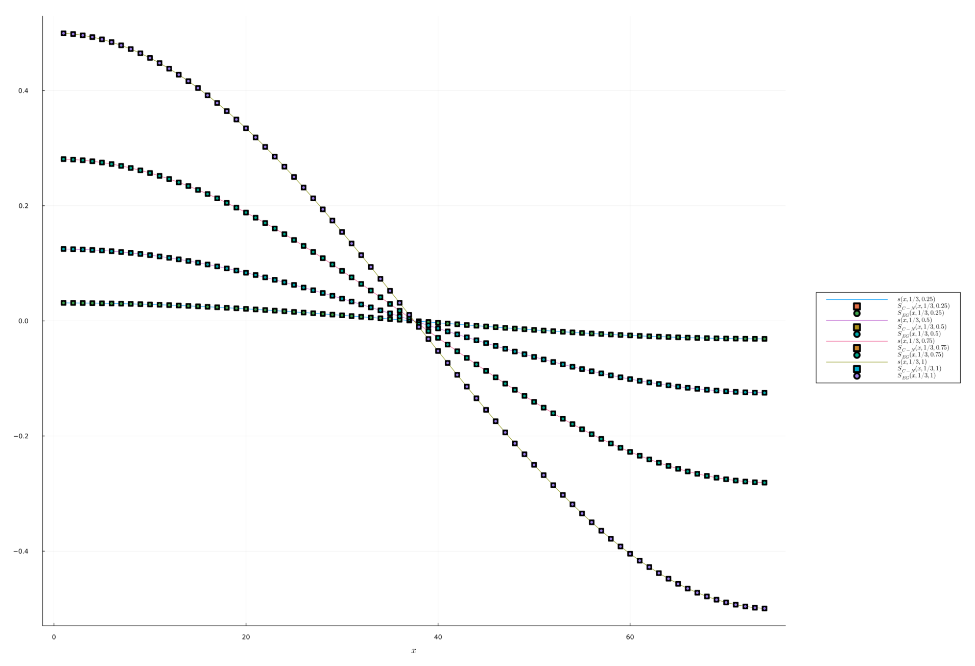
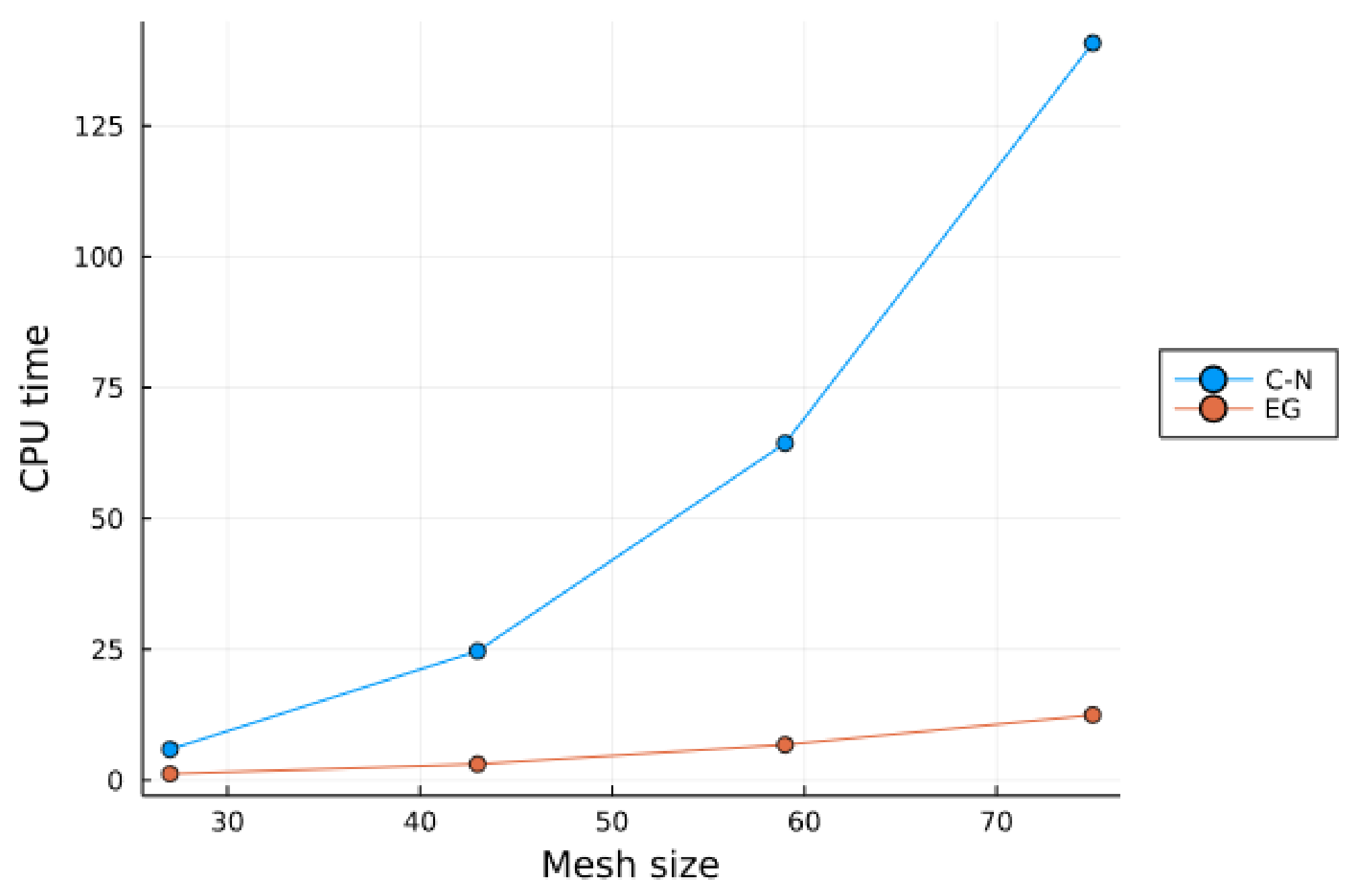
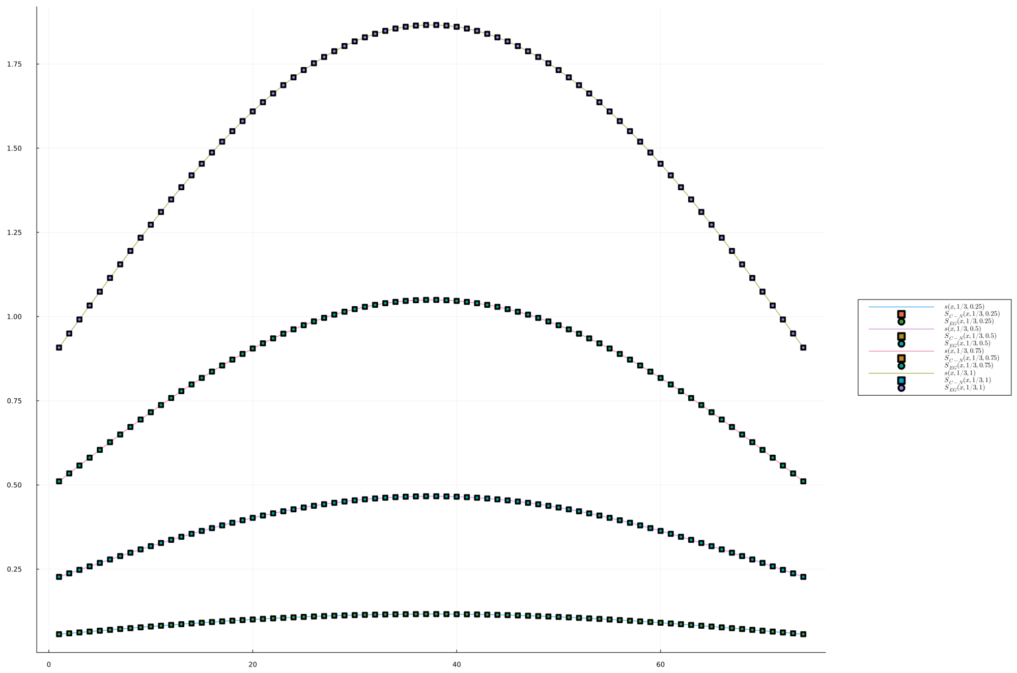
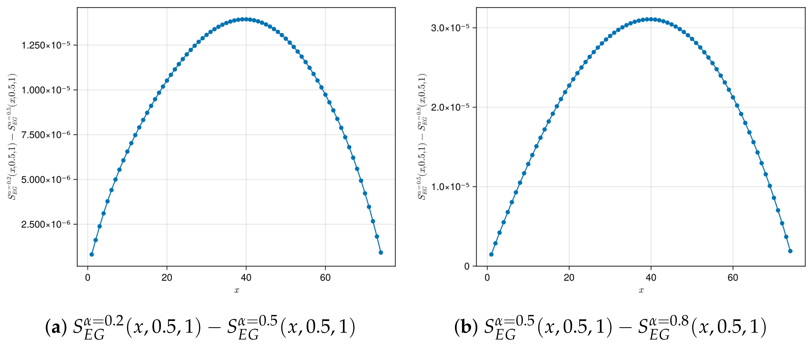
From Table 1 and Table 2, we observe that the C-N and the EG methods have similar accuracy, and their solutions converge to the exact solution as the spatial and temporal step sizes decrease. At the same time, the EG method notably converges to the exact solution much faster than the C-N method. For instance, at $\alpha (x,y,t)={\displaystyle \frac{10-y^2+t^4}{100}}$, it only takes 9.94 s for the EG method to achieve accuracy of $L_{\infty }=1.3527\times {10}^{-4}$, while it requires 116.84 s for the C-N method to achieve similar accuracy. To further illustrate the efficiency of the EG method, we plot in Figure 3 the CPU time of the EG and C-N methods against several spatial step sizes while fixing all other parameters. Figure 4 depicts a comparison between the exact solution and the numerical solutions of the proposed methods at $\alpha (x,y,t)={\displaystyle \frac{12-{cos}^3\left(xyt\right)}{13}}$, $h={\displaystyle \frac{1}{70}}$, $N=100$, $y={\displaystyle \frac{1}{3}}$, and $T=0.25,0.50,0.75,$ and $1.00$. These figures indicate the accuracy of the proposed methods and illustrate the computational superiority of the EG method over the C-N method. Figure 5 investigates the memory effect of the fractional derivative by plotting the difference between solution profiles at $\alpha =0.2$, 0.5, and 0.8 using the EG method with $y=0.5$, $T=1$, $h={\displaystyle \frac{1}{75}}$, and $N=100$. The solution values are seen to decrease as the value of $\alpha$ increases from 0.2 to 0.8.

Example 2.

We investigate the numerical solution of the two-dimensional VO-TFADRE (1) with the exact solution written as

$$s(x,y,t)=t^{2}cos\left(\pi x\right)cos\left(\pi y\right),$$

(33)

with the source term $g(x,y,t)$ expressed as

$$\begin{array}{cc}\hfill g(x,y,t)& ={\displaystyle \frac{2t^{2-\alpha (x,y,t)}}{\Gamma (3-\alpha (x,y,t\left)\right)}}cos\left(\pi x\right)cos\left(\pi y\right)+t^2\pi (2\pi cos\left(\pi x\right)cos\left(\pi y\right)\hfill \\ \hfill & -cos\left(\pi x\right)sin\left(\pi y\right)-cos\left(\pi y\right)sin\left(\pi x\right))+t^{2}cos\left(\pi x\right)cos\left(\pi y\right).\hfill \end{array}$$

(34)

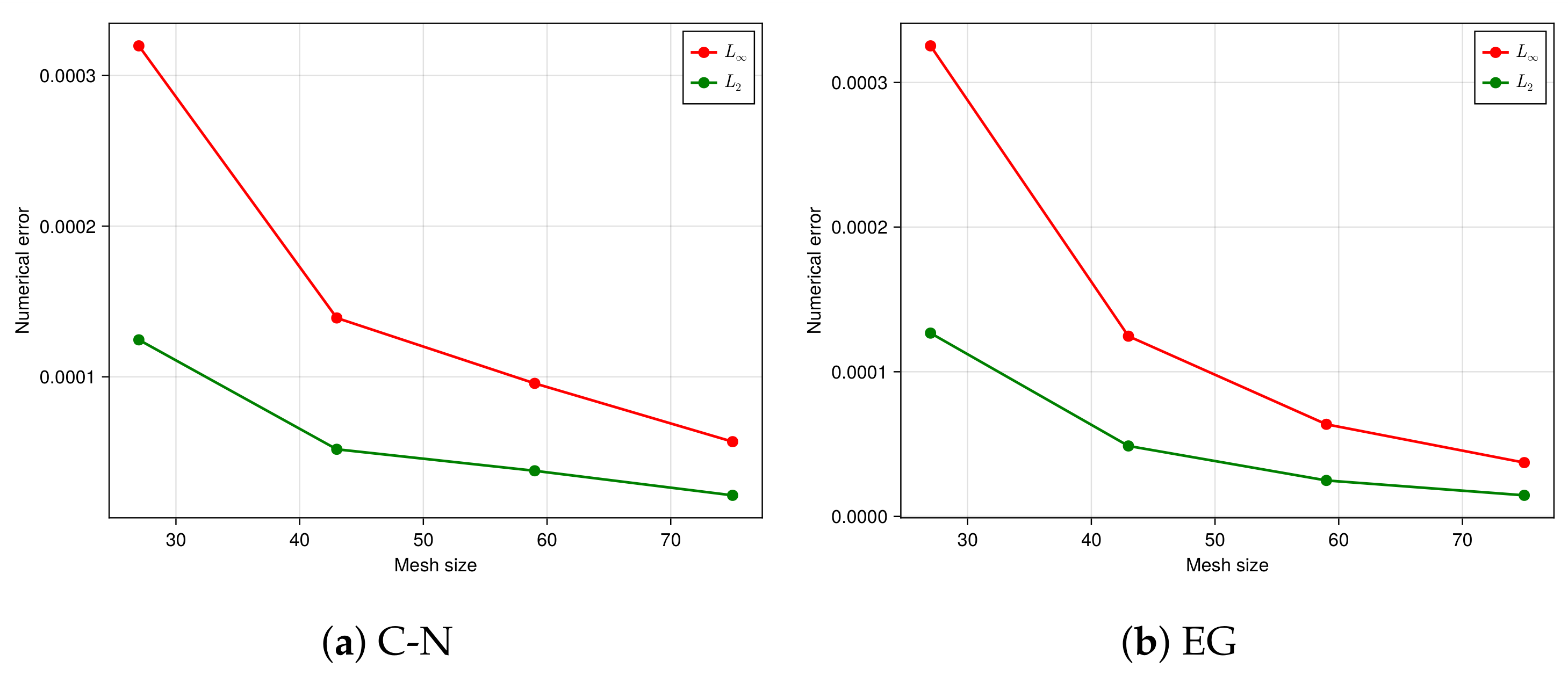
We can easily obtain the initial and boundary conditions from Equation (33). To investigate the performance of the proposed methods, we set $\Omega =[0,1]\times [0,1]$ and $T=1$. The current example records observations similar to the previous test problem.

Table 3. Errors and CPU times of the EG and the C-N methods for solving Example 2 with fixed time increment $\tau ={\displaystyle \frac{1}{100}}$.

		C-N			EG
$\mathbf{\alpha }(\mathit{x},\mathit{y},\mathit{t})$	${\mathit{h}}^{-\mathbf{1}}$	CPU Time	${\mathit{L}}_{\infty }$	Average Err.	CPU Time	${\mathit{L}}_{\infty }$	Average Err.
${\displaystyle \frac{e^{xyt}+cos\left(xyt\right)}{27}}$	27	5.25	3.2397 $\times {10}^{-4}$	1.0587 $\times {10}^{-4}$	1.09	3.3001 $\times {10}^{-4}$	1.0763 $\times {10}^{-4}$
	43	21.85	1.3253 $\times {10}^{-4}$	4.2451 $\times {10}^{-5}$	2.59	1.2898 $\times {10}^{-4}$	4.0603 $\times {10}^{-5}$
	59	58.77	8.1416 $\times {10}^{-5}$	2.2493 $\times {10}^{-5}$	5.80	6.7984 $\times {10}^{-5}$	2.0928 $\times {10}^{-5}$
	75	136.84	6.5714 $\times {10}^{-5}$	2.7492 $\times {10}^{-5}$	11.40	4.1460 $\times {10}^{-5}$	1.2908 $\times {10}^{-5}$
${\displaystyle \frac{18-e^{xyt}}{19}}$	27	1.94	4.0876 $\times {10}^{-4}$	2.0961 $\times {10}^{-4}$	0.68	3.1857 $\times {10}^{-4}$	1.0284 $\times {10}^{-4}$
	43	8.08	1.9259 $\times {10}^{-4}$	1.3193 $\times {10}^{-4}$	1.94	1.1953 $\times {10}^{-4}$	3.7648 $\times {10}^{-5}$
	59	22.08	1.3175 $\times {10}^{-4}$	9.9992 $\times {10}^{-5}$	5.17	5.9277 $\times {10}^{-5}$	1.8853 $\times {10}^{-5}$
	75	48.55	1.1034 $\times {10}^{-4}$	7.9912 $\times {10}^{-5}$	7.52	3.3077 $\times {10}^{-5}$	1.1503 $\times {10}^{-5}$
${\displaystyle \frac{15+{\left(xy\right)}^5-{\left(yt\right)}^6}{70}}$	27	2.47	3.3237 $\times {10}^{-4}$	1.2109 $\times {10}^{-4}$	0.56	3.2376 $\times {10}^{-4}$	1.0640 $\times {10}^{-4}$
	43	11.67	1.3229 $\times {10}^{-4}$	5.0923 $\times {10}^{-5}$	1.67	1.2334 $\times {10}^{-4}$	3.9511 $\times {10}^{-5}$
	59	27.50	7.7299 $\times {10}^{-5}$	2.9287 $\times {10}^{-5}$	4.21	6.2591 $\times {10}^{-5}$	1.9763 $\times {10}^{-5}$
	75	60.53	5.3527 $\times {10}^{-5}$	2.8376 $\times {10}^{-5}$	8.72	3.6157 $\times {10}^{-5}$	1.1631 $\times {10}^{-5}$
${\displaystyle \frac{8-\left(xyt\right)+cos\left(xyt\right)}{19}}$	27	3.23	3.2751 $\times {10}^{-4}$	1.3130 $\times {10}^{-4}$	0.86	3.2312 $\times {10}^{-4}$	1.0578 $\times {10}^{-4}$
	43	14.09	1.5672 $\times {10}^{-4}$	5.4777 $\times {10}^{-5}$	2.14	1.2293 $\times {10}^{-4}$	3.9207 $\times {10}^{-5}$
	59	37.11	7.8307 $\times {10}^{-5}$	3.1249 $\times {10}^{-5}$	5.18	6.2282 $\times {10}^{-5}$	1.9640 $\times {10}^{-5}$
	75	78.79	6.8919 $\times {10}^{-5}$	2.4045 $\times {10}^{-5}$	9.45	3.5892 $\times {10}^{-5}$	1.1639 $\times {10}^{-5}$
${\displaystyle \frac{5+{\left(yt\right)}^4-{\left(xy\right)}^6}{40}}$	27	5.80	3.6905 $\times {10}^{-4}$	1.1172 $\times {10}^{-4}$	0.82	3.2799 $\times {10}^{-4}$	1.0744 $\times {10}^{-4}$
	43	25.03	1.2097 $\times {10}^{-4}$	4.1625 $\times {10}^{-5}$	3.05	1.2709 $\times {10}^{-4}$	4.0414 $\times {10}^{-5}$
	59	67.53	6.9442 $\times {10}^{-5}$	2.2267 $\times {10}^{-5}$	6.29	6.6105 $\times {10}^{-5}$	2.0644 $\times {10}^{-5}$
	75	147.31	5.8311 $\times {10}^{-5}$	2.9765 $\times {10}^{-5}$	10.90	3.9612 $\times {10}^{-5}$	1.2513 $\times {10}^{-5}$
${\displaystyle \frac{10+y^4+t^4}{30}}$	27	4.59	3.4782 $\times {10}^{-4}$	1.6859 $\times {10}^{-4}$	0.67	3.2346 $\times {10}^{-4}$	1.0628 $\times {10}^{-4}$
	43	20.19	1.4581 $\times {10}^{-4}$	5.1795 $\times {10}^{-5}$	2.02	1.2314 $\times {10}^{-4}$	3.9424 $\times {10}^{-5}$
	59	54.88	7.8306 $\times {10}^{-5}$	3.0053 $\times {10}^{-5}$	5.05	6.2434 $\times {10}^{-5}$	1.9707 $\times {10}^{-5}$
	75	112.26	5.8874 $\times {10}^{-5}$	2.3807 $\times {10}^{-5}$	9.09	3.6021 $\times {10}^{-5}$	1.1595 $\times {10}^{-5}$

and

Table 4. Errors and CPU times of the EG and the C-N methods for solving Example 2 with fixed spatial step size $h={\displaystyle \frac{1}{83}}$.

		C-N			EG
$\mathbf{\alpha }(\mathit{x},\mathit{y},\mathit{t})$	${\mathit{\tau }}^{-\mathbf{1}}$	CPU Time	${\mathit{L}}_{\infty }$	Average Err.	CPU Time	${\mathit{L}}_{\infty }$	Average Err.
0.3	8	4.41	1.9851 $\times {10}^{-3}$	9.9237 $\times {10}^{-4}$	0.59	1.9799 $\times {10}^{-3}$	9.8993 $\times {10}^{-4}$
	16	8.23	4.9935 $\times {10}^{-4}$	2.4338 $\times {10}^{-4}$	1.19	4.9937 $\times {10}^{-4}$	2.4069 $\times {10}^{-4}$
	32	16.85	1.2392 $\times {10}^{-4}$	5.6604 $\times {10}^{-5}$	3.13	1.2617 $\times {10}^{-4}$	5.2585 $\times {10}^{-5}$
	64	32.69	3.4280 $\times {10}^{-5}$	1.9360 $\times {10}^{-5}$	7.10	3.1945 $\times {10}^{-5}$	1.1519 $\times {10}^{-5}$
	128	62.12	4.3125 $\times {10}^{-5}$	1.7704 $\times {10}^{-5}$	16.10	3.0975 $\times {10}^{-5}$	9.7545 $\times {10}^{-6}$
0.7	8	4.87	1.9561 $\times {10}^{-3}$	1.0694 $\times {10}^{-3}$	0.56	1.9532 $\times {10}^{-3}$	1.0641 $\times {10}^{-3}$
	16	7.18	4.9319 $\times {10}^{-4}$	2.7270 $\times {10}^{-4}$	1.54	4.9553 $\times {10}^{-4}$	2.6554 $\times {10}^{-4}$
	32	12.35	1.2503 $\times {10}^{-4}$	6.5465 $\times {10}^{-5}$	2.87	1.2686 $\times {10}^{-4}$	6.0948 $\times {10}^{-5}$
	64	18.94	5.1131 $\times {10}^{-5}$	2.7179 $\times {10}^{-5}$	6.26	3.2756 $\times {10}^{-5}$	1.3899 $\times {10}^{-5}$
	128	37.08	9.5832 $\times {10}^{-5}$	4.6902 $\times {10}^{-5}$	11.55	2.9206 $\times {10}^{-5}$	9.5009 $\times {10}^{-6}$
${\displaystyle \frac{18-e^{xyt}}{19}}$	8	12.30	1.7765 $\times {10}^{-3}$	1.0672 $\times {10}^{-3}$	0.64	1.7814 $\times {10}^{-3}$	1.0570 $\times {10}^{-3}$
	16	18.26	4.2398 $\times {10}^{-4}$	2.6015 $\times {10}^{-4}$	1.42	4.2586 $\times {10}^{-4}$	2.6066 $\times {10}^{-4}$
	32	45.98	9.8846 $\times {10}^{-5}$	6.5554 $\times {10}^{-5}$	2.88	1.0001 $\times {10}^{-4}$	6.0937 $\times {10}^{-5}$
	64	64.38	7.9478 $\times {10}^{-5}$	6.1432 $\times {10}^{-5}$	6.18	2.3326 $\times {10}^{-5}$	1.4284 $\times {10}^{-5}$
	128	103.24	1.0388 $\times {10}^{-4}$	8.0312 $\times {10}^{-5}$	15.76	2.8453 $\times {10}^{-5}$	9.3983 $\times {10}^{-6}$

present CPU time and errors in solving Example 2 using both the C-N and EG methods with fixed time increment and fixed spatial step size, respectively. We observe that the errors decrease as the sizes of the time and space partitions decrease. Figure 6 compares the exact solution and the numerical solutions of the proposed methods at $\alpha (x,y,t)={\displaystyle \frac{10+y^4+t^4}{30}}$, $h=1/75$, $N=100$, $y={\displaystyle \frac{1}{3}}$, and $T=0.25,0.50,0.75,1.00$. In Figure 7, we sketch the $L_{\infty }$ and $L_2$ errors against several mesh sizes while fixing the remaining parameters. From this figure, it can be seen that numerical errors decrease steadily with finer meshes, which confirms the convergence of the proposed methods. From Table 3 and Table 4 and Figure 7, one can see that the EG method results in considerable savings of CPU time while maintaining comparable accuracy as compared to the C-N method. Again, the tabulated and graphical results demonstrate that the C-N and EG methods are accurate, and the latter is much faster than the former in solving the considered problem.

Table 5. Errors and computational orders of the EG method for solving Examples 1 and 2 with $\tau ={\displaystyle \frac{1}{100}}$ and $\alpha (x,y,t)={\displaystyle \frac{10-y^2+t^4}{100}}$.

Example	${\mathit{h}}^{-1}$	${\mathit{L}}_{\mathit{\infty }}$	Computational Order
1	27	1.2490 $\times {10}^{-3}$
	43	4.8759 $\times {10}^{-4}$	2.02
	59	2.3573 $\times {10}^{-4}$	2.29
	75	1.4143 $\times {10}^{-4}$	2.12
2	27	3.2905 $\times {10}^{-4}$
	43	1.2806 $\times {10}^{-4}$	2.02
	59	6.7058 $\times {10}^{-5}$	2.04
	75	4.0551 $\times {10}^{-5}$	2.09

demonstrates the computational convergence orders of the EG method using the formula: $\mathrm{computational}\mathrm{order}=log\left(L_{\infty }(\tau ,h_1)/L_{\infty }(\tau ,h_2)\right)/log(h_1/h_2)$. From this table, it can be observed that the computational orders are in good agreement with the theoretical considerations.

Table 6. CPU time and speedup of EG method compared to C-N scheme for Example 2 with $\alpha (x,y,t)={\displaystyle \frac{7-{\left(xyt\right)}^4+{sin}^3\left(xyt\right)}{15}}$, $T=1$, and $N=100$.

${\mathit{h}}^{-1}$	43	59	75	91	107	123	139
C-N	8.61	25.41	43.72	77.41	127.17	220.92	319.52
EG	1.20	3.79	7.08	11.2	15.96	20.16	40.66
speedup	7.18	6.70	6.18	6.91	7.97	10.96	7.86

demonstrates the speedup results of the EG method compared to the C-N difference scheme for solving Example 2. It can be observed that the EG method is more efficient with considerable savings in computational time compared to the C-N scheme. To further enhance this efficiency, a parallel version of the EG method is proposed in the next section.

5. Parallel Implementation and Numerical Simulations

5.1. Parallel Implementation

Parallel computing is a well-known strategy for diminishing computational burdens by performing many arithmetic operations simultaneously. It has been a vital component of large-scale applications and algorithms in engineering and science, such as large sparse linear systems, computational fluid dynamics, and neutron transport (see [51,52] and references therein). The goal of this part is to accelerate the EG method further with parallel computing.

As discussed earlier, the application of the EG scheme (11) to the VO-TFADRE will lead to a large sparse linear system to be solved at each time step. Such linear systems are solved via the serial algorithm described in Algorithm 1. From Step 1 of the serial algorithm, it can be observed that the calculation of the residual vectors ${\mathbf{r}}_0={\mathbf{b}}^k-A_k{\mathbf{S}}_0^{k+1}$, $0\le k\le N-1$ requires storing and processing the solution values at all previous time levels. In other words, Step 1 requires $O\left(k\right)$ computational cost at each time level k and $O\left(N^2\right)$ computational cost for the entire process. As a result, the calculation of Step 1 is one of the most time-consuming parts of the serial solution. Hence, it is worthwhile to parallelize Step 1 to further enhance the performance. To this end, we use a non-overlapping domain decomposition strategy to calculate the residual vectors ${\mathbf{r}}_0={\mathbf{b}}^k-A_k{\mathbf{S}}_0^{k+1}$, $0\le k\le N-1$.

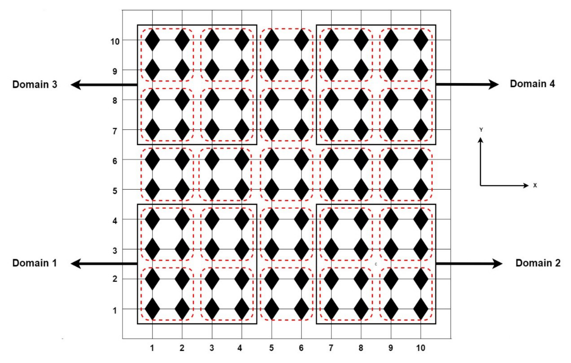
A domain decomposition strategy partitions the computing domain into multiple subdomains, each of which can be handled independently. Here, we divide the spatial domain $\Omega$ at each time level into non-overlapped subdomains ${\Omega }_D,D=1,2,\dots ,z$. Figure 8 shows the case for $z=4$. From the same figure, it can be seen that the subdomains are separated by block interfaces, where each block contains groups of four grid points. The residual values at the groups of each subdomain are computed concurrently using different threads based on Equation (11). The residual values in the interface blocks that separate the subdomains are also calculated with the help of Equation (11). For convenience, the parallel EG (ParEG) algorithm for solving the VO-TFADRE (1) is described in Algorithm 2. All numerical simulations will be performed using multi-threading environment in Julia.

Algorithm 2 Parallel algorithm of the EG method

1. At each time level k, $k=0,1,\dots ,N-1$, choose an initial guess ${\mathbf{S}}_0^{k+1}$ and a. Compute the residual values in the interface blocks that separate the subdomains using Equation (11). b. Compute the residual values at the groups of each subdomain concurrently using different threads based on Equation (11). Afterwards, perform the steps 2 to 5. 2. Define ${\tilde{\mathbf{r}}}_0$ as an arbitrary vector such that $<{\tilde{\mathbf{r}}}_0,{\mathbf{r}}_0>\ne 0$, e.g., ${\tilde{\mathbf{r}}}_0={\mathbf{r}}_0$. 3. Initialize the vectors ${\mathbf{v}}_0={\mathbf{d}}_0=0.$ 4. Initialize the constants ${\rho }_0=\kappa ={\omega }_0=1$. 5. for $n=1,2,\dots$ do          ${\rho }_n=<{\mathbf{r}}_{n-1},{\tilde{\mathbf{r}}}_0>,$          ${\beta }_n=({\rho }_n/{\rho }_{n-1})(\kappa /{\omega }_{n-1}),$          ${\mathbf{d}}_n={\mathbf{r}}_{n-1}+\beta ({\mathbf{d}}_{n-1}+{\omega }_{n-1}{\mathbf{v}}_{n-1}),$          ${\mathbf{v}}_n=A_k{\mathbf{d}}_n,$          $\kappa ={\rho }_n/<{\tilde{\mathbf{r}}}_0,{\mathbf{v}}_n>,$          $\mathbf{e}={\mathbf{r}}_{n-1}-\kappa {\mathbf{v}}_n,$          $\mathbf{f}=A_k\mathbf{e},$          ${\omega }_n=<\mathbf{f},\mathbf{e}>/<\mathbf{f},\mathbf{f}>,$          ${\mathbf{S}}_n^{k+1}={\mathbf{S}}_{n-1}^{k+1}+\kappa {\mathbf{d}}_n+{\omega }_n\mathbf{e},$          if $\left|\right|{\mathbf{S}}_n^{k+1}-{\mathbf{S}}_{n-1}^{k+1}{\left|\right|}_{\infty }<Tolerance$          break          else          ${\mathbf{r}}_n=\mathbf{e}-{\omega }_n\mathbf{f},$ end do 6. Print solution vectors ${\mathbf{S}}^{\mathbf{k}+\mathbf{1}}$, $k=0,1,\dots ,N-1$.

5.2. Numerical Simulations

In this part, we investigate the performance of the ParEG method in solving the VO-TFADRE (1). We solve Examples 1 and 2 given in Section 4, and use the EG method as a benchmark to compare with. We run numerical simulations with stopping criterion $\left|\right|{\mathbf{S}}_n^{k+1}-{\mathbf{S}}_{n-1}^{k+1}{\left|\right|}_{\infty }<{10}^{-5}$ and domain $\Omega =[0,1]\times [0,1]$. All codes are implemented using the Julia multi-threading environment and run on a computer with the following specifications: Intel(R) Core(TM) i7-8550 CPU with 8 GB of RAM and Windows 10 operating system.

Table 7. Errors and CPU times of the ParEG and the EG methods for solving Example 1 with $\tau ={\displaystyle \frac{1}{100}}$, $T=1$, and $z=4$.

		EG			ParEG
$\mathbf{\alpha }(\mathit{x},\mathit{y},\mathit{t})$	${\mathit{h}}^{-\mathbf{1}}$	CPU Time	${\mathit{L}}_{\infty }$	Average Err.	CPU Time	${\mathit{L}}_{\infty }$	Average Err.
${\displaystyle \frac{10-y^2+t^4}{100}}$	75	12.30	1.3527 $\times {10}^{-4}$	4.4200 $\times {10}^{-5}$	10.44	1.3527 $\times {10}^{-3}$	4.4200 $\times {10}^{-4}$
	83	14.47	1.0534 $\times {10}^{-4}$	3.6115 $\times {10}^{-5}$	13.60	1.0534 $\times {10}^{-4}$	3.6115 $\times {10}^{-5}$
	91	19.84	8.2959 $\times {10}^{-5}$	3.0577 $\times {10}^{-5}$	17.45	8.2959 $\times {10}^{-5}$	3.0577 $\times {10}^{-5}$
	115	39.10	6.6530 $\times {10}^{-5}$	2.2662 $\times {10}^{-5}$	34.28	6.6530 $\times {10}^{-5}$	2.2662 $\times {10}^{-5}$
${\displaystyle \frac{15-sin{\left(xyt\right)}^2}{15}}$	75	8.86	1.2294 $\times {10}^{-4}$	3.8373 $\times {10}^{-5}$	6.75	1.2294 $\times {10}^{-4}$	3.8373 $\times {10}^{-5}$
	83	9.61	9.4340 $\times {10}^{-5}$	3.1122 $\times {10}^{-5}$	7.73	9.4340 $\times {10}^{-5}$	3.1122 $\times {10}^{-5}$
	91	12.62	7.2981 $\times {10}^{-5}$	2.6222 $\times {10}^{-5}$	10.71	7.2981 $\times {10}^{-5}$	2.6222 $\times {10}^{-5}$
	115	23.10	3.3706 $\times {10}^{-5}$	1.9579 $\times {10}^{-5}$	17.39	3.3706 $\times {10}^{-5}$	1.9579 $\times {10}^{-5}$
${\displaystyle \frac{17+cos{\left(xt\right)}^5}{18}}$	75	10.50	1.1202 $\times {10}^{-4}$	3.5713 $\times {10}^{-5}$	9.50	1.1202 $\times {10}^{-4}$	3.5713 $\times {10}^{-5}$
	83	13.98	8.3610 $\times {10}^{-5}$	2.9049 $\times {10}^{-5}$	10.28	8.3610 $\times {10}^{-5}$	2.9049 $\times {10}^{-5}$
	91	16.24	6.2494 $\times {10}^{-5}$	2.4830 $\times {10}^{-5}$	13.50	6.2494 $\times {10}^{-5}$	2.4830 $\times {10}^{-5}$
	115	31.89	2.9916 $\times {10}^{-5}$	2.0751 $\times {10}^{-5}$	23.31	2.9916 $\times {10}^{-5}$	2.0751 $\times {10}^{-5}$
${\displaystyle \frac{10+y^4+t^6}{90}}$	75	12.35	1.3321 $\times {10}^{-4}$	4.3634 $\times {10}^{-5}$	11.04	1.3321 $\times {10}^{-4}$	4.3634 $\times {10}^{-5}$
	83	15.89	1.0332 $\times {10}^{-4}$	3.5586 $\times {10}^{-5}$	13.74	1.0332 $\times {10}^{-4}$	3.5586 $\times {10}^{-5}$
	91	21.40	8.0972 $\times {10}^{-5}$	3.0081 $\times {10}^{-5}$	19.12	8.0972 $\times {10}^{-5}$	3.0081 $\times {10}^{-5}$
	115	40.58	6.6742 $\times {10}^{-5}$	2.2308 $\times {10}^{-5}$	35.91	6.6742 $\times {10}^{-5}$	2.2308 $\times {10}^{-5}$
${\displaystyle \frac{12-cos{\left(xyt\right)}^3}{13}}$	75	9.61	8.3883 $\times {10}^{-5}$	4.9545 $\times {10}^{-5}$	8.46	8.3883 $\times {10}^{-5}$	4.9545 $\times {10}^{-5}$
	83	11.12	7.2988 $\times {10}^{-5}$	4.7436 $\times {10}^{-5}$	9.85	7.2988 $\times {10}^{-5}$	4.7436 $\times {10}^{-5}$
	91	16.50	7.3304 $\times {10}^{-5}$	4.7625 $\times {10}^{-5}$	13.67	7.3304 $\times {10}^{-5}$	4.7625 $\times {10}^{-5}$
	115	29.81	7.4016 $\times {10}^{-5}$	5.4817 $\times {10}^{-5}$	22.68	7.4016 $\times {10}^{-5}$	5.4817 $\times {10}^{-5}$
${\displaystyle \frac{7-{\left(xyt\right)}^4+sin{\left(xyt\right)}^3}{15}}$	75	15.35	1.1704 $\times {10}^{-4}$	4.1977 $\times {10}^{-5}$	11.94	1.1704 $\times {10}^{-4}$	4.1977 $\times {10}^{-5}$
	83	19.79	8.7667 $\times {10}^{-5}$	3.5463 $\times {10}^{-5}$	13.77	8.7667 $\times {10}^{-5}$	3.5463 $\times {10}^{-5}$
	91	25.87	6.9055 $\times {10}^{-5}$	3.1416 $\times {10}^{-5}$	18.32	6.9055 $\times {10}^{-5}$	3.1416 $\times {10}^{-5}$
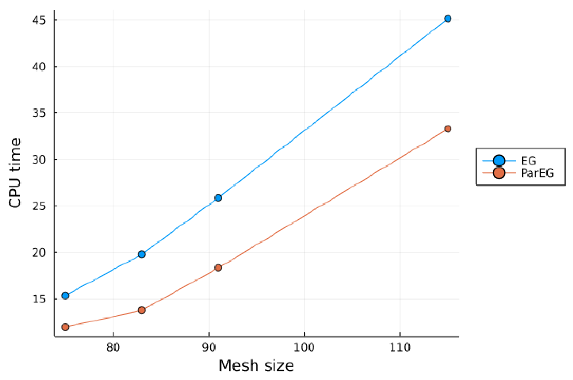
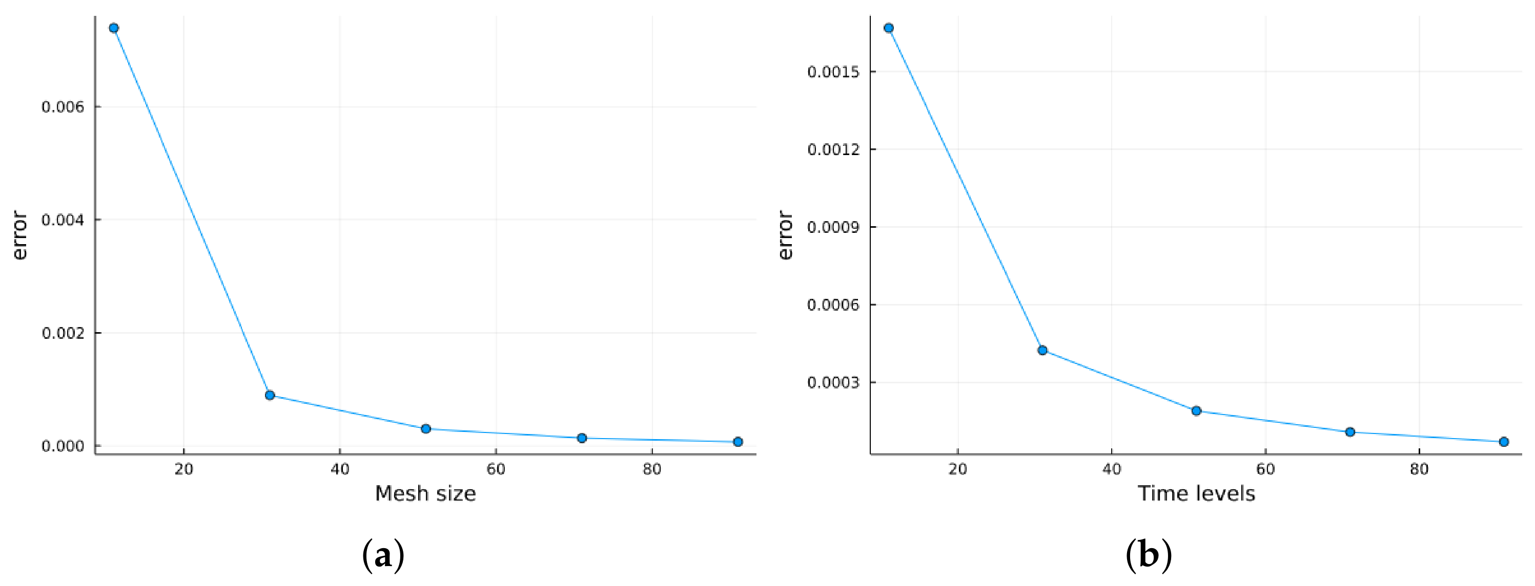
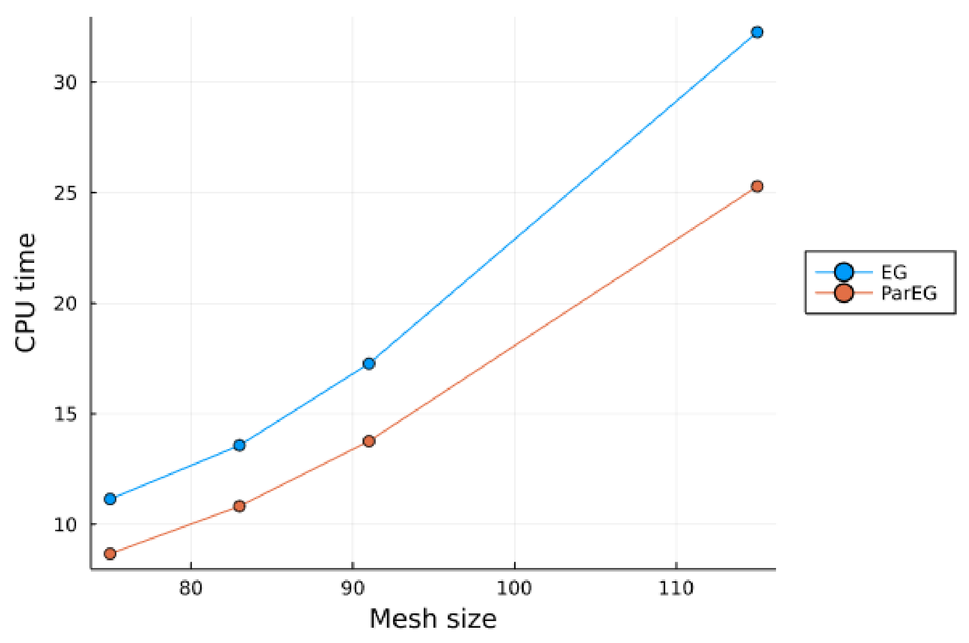
	115	45.14	6.9063 $\times {10}^{-5}$	2.7660 $\times {10}^{-5}$	33.28	6.9063 $\times {10}^{-5}$	2.7660 $\times {10}^{-5}$

shows CPU time, maximum absolute error, and average error of solving Example 1 using the EG and ParEG methods. One can easily see that the accuracy of the parallel solution is the same as the serial solution. We observe that the ParEG method requires less CPU time in solving the considered problem as compared to the EG method. Figure 9 plots the maximum error against several mesh sizes and time steps for solving Example 1 using the ParEG method. We observe that the errors decrease as the spatial and temporal step sizes decrease. Figure 10 demonstrates the CPU time of the ParEG and EG methods versus various mesh sizes. Again, one can see that the ParEG method is faster than the EG method.

Table 8. Errors and CPU times of the ParEG and the EG methods for solving Example 2 with $\tau ={\displaystyle \frac{1}{100}}$, $T=1$, and $z=4$.

		EG			ParEG
$\mathbf{\alpha }(\mathit{x},\mathit{y},\mathit{t})$	${\mathit{h}}^{-\mathbf{1}}$	CPU Time	${\mathit{L}}_{\infty }$	Average Err.	CPU Time	${\mathit{L}}_{\infty }$	Average Err.
${\displaystyle \frac{e^{xyt}+cos\left(xyt\right)}{27}}$	75	11.14	4.0831 $\times {10}^{-5}$	1.2769 $\times {10}^{-5}$	8.67	4.0831 $\times {10}^{-5}$	1.2769 $\times {10}^{-5}$
	83	13.57	3.2967 $\times {10}^{-5}$	1.0543 $\times {10}^{-5}$	10.82	3.2967 $\times {10}^{-5}$	1.0543 $\times {10}^{-5}$
	91	17.27	2.7062 $\times {10}^{-5}$	8.9764 $\times {10}^{-6}$	13.76	2.7062 $\times {10}^{-5}$	8.9764 $\times {10}^{-6}$
	115	32.26	1.6139 $\times {10}^{-5}$	6.5334 $\times {10}^{-6}$	25.28	1.6139 $\times {10}^{-5}$	6.5334 $\times {10}^{-6}$
${\displaystyle \frac{18-e^{xyt}}{19}}$	75	7.62	3.3077 $\times {10}^{-5}$	1.1503 $\times {10}^{-5}$	6.42	3.3077 $\times {10}^{-5}$	1.1503 $\times {10}^{-5}$
	83	9.62	2.5278 $\times {10}^{-5}$	9.5985 $\times {10}^{-6}$	7.95	2.5278 $\times {10}^{-5}$	9.5985 $\times {10}^{-6}$
	91	12.29	1.9452 $\times {10}^{-5}$	8.3530 $\times {10}^{-6}$	9.67	1.9452 $\times {10}^{-5}$	8.3530 $\times {10}^{-6}$
	115	22.59	9.5036 $\times {10}^{-6}$	6.8582 $\times {10}^{-6}$	17.62	9.5036 $\times {10}^{-6}$	6.8582 $\times {10}^{-6}$
${\displaystyle \frac{15+{\left(xy\right)}^5-{\left(yt\right)}^6}{70}}$	75	9.25	3.7241 $\times {10}^{-5}$	1.1931 $\times {10}^{-5}$	8.49	3.7241 $\times {10}^{-5}$	1.1931 $\times {10}^{-5}$
	83	12.11	2.9387 $\times {10}^{-5}$	9.6216 $\times {10}^{-6}$	10.76	2.9387 $\times {10}^{-5}$	9.6216 $\times {10}^{-6}$
	91	15.57	2.3491 $\times {10}^{-5}$	7.9801 $\times {10}^{-6}$	13.7	2.3491 $\times {10}^{-5}$	7.9801 $\times {10}^{-6}$
	115	30.4	1.2917 $\times {10}^{-5}$	5.3534 $\times {10}^{-6}$	26.00	1.2917 $\times {10}^{-5}$	5.3534 $\times {10}^{-6}$
${\displaystyle \frac{8-\left(xyt\right)+cos\left(xyt\right)}{19}}$	75	9.56	3.5892 $\times {10}^{-5}$	1.1639 $\times {10}^{-5}$	8.64	3.5892 $\times {10}^{-5}$	1.1639 $\times {10}^{-5}$
	83	12.29	2.8032 $\times {10}^{-5}$	9.4329 $\times {10}^{-6}$	10.83	2.8032 $\times {10}^{-5}$	9.4329 $\times {10}^{-6}$
	91	15.73	2.2174 $\times {10}^{-5}$	7.8938 $\times {10}^{-6}$	14.07	2.2174 $\times {10}^{-5}$	7.8938 $\times {10}^{-6}$
	115	30.35	1.3945 $\times {10}^{-5}$	5.5440 $\times {10}^{-6}$	26.39	1.3945 $\times {10}^{-5}$	5.5440 $\times {10}^{-6}$
${\displaystyle \frac{5+{\left(yt\right)}^4-{\left(xy\right)}^6}{40}}$	75	10.04	3.9612 $\times {10}^{-5}$	1.2513 $\times {10}^{-5}$	9.36	3.9612 $\times {10}^{-5}$	1.2513 $\times {10}^{-5}$
	83	12.81	3.1745 $\times {10}^{-5}$	1.0243 $\times {10}^{-5}$	11.79	3.1745 $\times {10}^{-5}$	1.0243 $\times {10}^{-5}$
	91	16.84	2.5839 $\times {10}^{-5}$	8.6346 $\times {10}^{-6}$	15.19	2.5839 $\times {10}^{-5}$	8.6346 $\times {10}^{-6}$
	115	32.87	1.4924 $\times {10}^{-5}$	6.0643 $\times {10}^{-6}$	30.19	1.4924 $\times {10}^{-5}$	6.0643 $\times {10}^{-6}$
${\displaystyle \frac{10+y^4+t^4}{30}}$	75	9.13	3.6021 $\times {10}^{-5}$	1.1595 $\times {10}^{-5}$	8.98	3.6021 $\times {10}^{-5}$	1.1595 $\times {10}^{-5}$
	83	11.59	2.8159 $\times {10}^{-5}$	9.3397 $\times {10}^{-6}$	11.27	2.8159 $\times {10}^{-5}$	9.3397 $\times {10}^{-6}$
	91	15.25	2.2298 $\times {10}^{-5}$	7.7572 $\times {10}^{-6}$	14.58	2.2298 $\times {10}^{-5}$	7.7572 $\times {10}^{-6}$
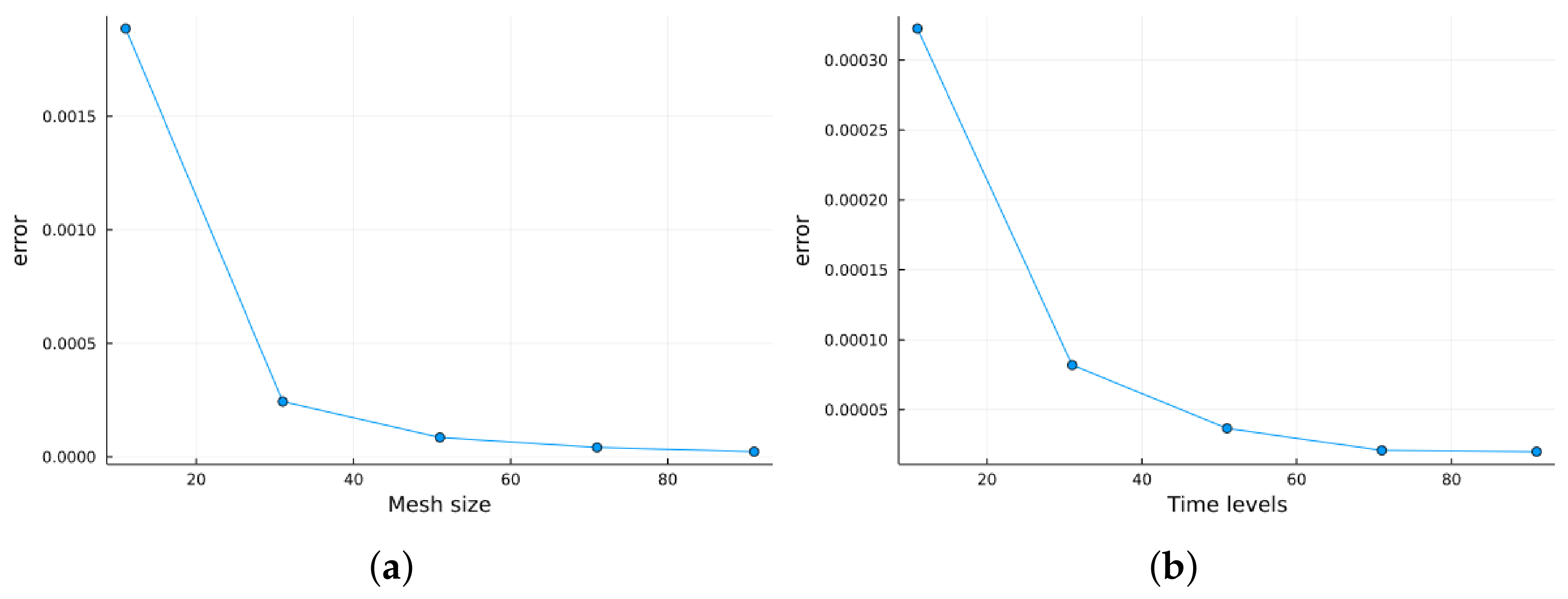
	115	30.15	1.3421 $\times {10}^{-5}$	5.2846 $\times {10}^{-6}$	28.04	1.3421 $\times {10}^{-5}$	5.2846 $\times {10}^{-6}$

compares the numerical results of solving Example 2 using the EG and ParEG methods. The data in the table show that the ParEG method has the same accuracy as the EG method, but takes less computing time in solving the considered problem. The effect of reducing spatial and temporal step sizes over the maximum error in solving Example 2 using ParEG method is depicted in Figure 11. It follows from this figure that the ParEG method converges to the exact solution as the spatial and temporal step sizes decrease. A comparison of computational time between the EG and ParEG methods for solving Example 2 is highlighted in Figure 12. Again, numerical results show that the ParEG method is a viable algorithm for accurate simulation of the considered problem with savings in computational cost as compared to the EG method.

6. Conclusions

This study has successfully addressed the numerical solution of the variable-order time fractional advection–diffusion–reaction in two space dimensions. By proposing a Crank–Nicolson discretization scheme based on central difference operators and the L1 formula for space and time variables, we developed a new algorithm, the EG method. The explicit group method, which utilizes a strategy of small fixed-size groups of mesh points, demonstrated computational advantages over the Crank–Nicolson scheme. Stability and convergence analyses were provided. The application of the proposed methods resulted in large sparse linear systems, efficiently solved using the Bi-CGSTAB method. Numerical experiments validated the accuracy of both the Crank–Nicolson and explicit group methods in simulating the variable-order time fractional advection–diffusion–reaction, with the explicit group method showing superior performance in terms of CPU time. To further reduce computational costs, we introduced a parallelized version of the explicit group method, which proved to be more efficient than the serial algorithm. Overall, the parallel algorithm offers a promising solution for efficiently solving the variable-order time fractional advection–diffusion–reaction and other high-dimensional fractional models [53,54] in the future.

In conclusion, the proposed explicit group method is computationally efficient, straightforward to implement, and well suited for parallelization. However, the history-dependent term remains computationally demanding, particularly for fine spatial meshes or long-time simulations. Further acceleration could be achieved by incorporating parallel-in-time strategies [55] for the considered model problem. In addition, model problems with confined or complex geometries [56] can also be investigated. The integration of such techniques within the current framework is an interesting direction for future work. The extension of this approach to nonlinear problems with optimal error analysis is another line of further studies. Finally, alternate C-N discretizations have been reported to improve stability and error estimates in integer-order models [57,58,59]. Extending such approaches to the variable-order fractional framework constitutes another interesting direction for future work.

References

1. Ezz-Eldien, S.S.; Doha, E.H.; Wang, Y.; Cai, W. A numerical treatment of the two-dimensional multi-term time-fractional mixed sub-diffusion and diffusion-wave equation. Commun. Nonlinear Sci. Numer. Simul. 2020, 91, 105445. [Google Scholar] [CrossRef] [Scilit]
2. Alsuyuti, M.M.; Doha, E.H.; Ezz-Eldien, S.S. Numerical simulation for classes of one-and two-dimensional multi-term time-fractional diffusion and diffusion-wave equation based on shifted Jacobi Galerkin scheme. Math. Methods Appl. Sci. 2025, 48, 8217–8244. [Google Scholar] [CrossRef] [Scilit]
3. Sun, H.; Zhang, Y.; Baleanu, D.; Chen, W.; Chen, Y. A new collection of real world applications of fractional calculus in science and engineering. Commun. Nonlinear Sci. Numer. Simul. 2018, 64, 213–231. [Google Scholar] [CrossRef] [Scilit]
4. Viera-Martin, E.; Gómez-Aguilar, J.; Solís-Pérez, J.; Hernández-Pérez, J.; Escobar-Jiménez, R. Artificial neural networks: A practical review of applications involving fractional calculus. Eur. Phys. J. Spec. Top. 2022, 231, 2059–2095. [Google Scholar] [CrossRef] [Scilit]
5. Arora, S.; Mathur, T.; Agarwal, S.; Tiwari, K.; Gupta, P. Applications of fractional calculus in computer vision: A survey. Neurocomputing 2022, 489, 407–428. [Google Scholar] [CrossRef] [Scilit]
6. Qiao, H.; Cheng, A. A fast modified L 1 finite difference method for time fractional diffusion equations with weakly singular solution. J. Appl. Math. Comput. 2024, 70, 3631–3660. [Google Scholar] [CrossRef] [Scilit]
7. Huang, C.; Yu, Y.; An, N.; Chen, H. A corrected Alikhanov scheme for a subdiffusion equation. Comput. Math. Appl. 2026, 207, 15–26. [Google Scholar] [CrossRef] [Scilit]
8. Liu, P.; Lei, M.; Hon, Y.C. An improved meshless finite integration method for the time fractional diffusion and high order equations. Math. Comput. Simul. 2025, 241, 15–39. [Google Scholar] [CrossRef] [Scilit]
9. Cao, Y.; Tan, Z. A space-time exponential convergence scheme for variable-coefficient time-fractional advection-diffusion-reaction equations based on double exponential transformation. Appl. Math. Comput. 2026, 516, 129876. [Google Scholar] [CrossRef] [Scilit]
10. Wang, W.; Balcerek, M.; Burnecki, K.; Chechkin, A.V.; Janušonis, S.; Ślęzak, J.; Vojta, T.; Wyłomańska, A.; Metzler, R. Memory-multi-fractional Brownian motion with continuous correlations. Phys. Rev. Res. 2023, 5, L032025. [Google Scholar] [CrossRef] [Scilit]
11. Cherstvy, A.G.; Thapa, S.; Mardoukhi, Y.; Chechkin, A.V.; Metzler, R. Time averages and their statistical variation for the Ornstein-Uhlenbeck process: Role of initial particle distributions and relaxation to stationarity. Phys. Rev. E 2018, 98, 022134. [Google Scholar] [CrossRef] [Scilit]
12. Salama, F.M. An efficient numerical treatment of variable-order time fractional advection–diffusion equation. Comput. Appl. Math. 2026, 45, 1–35. [Google Scholar] [CrossRef] [Scilit]
13. Salama, F.M. On numerical simulations of variable-order fractional cable equation arising in neuronal dynamics. Fractal Fract. 2024, 8, 282. [Google Scholar] [CrossRef] [Scilit]
14. Diethelm, K.; Kiryakova, V.; Luchko, Y.; Machado, J.T.; Tarasov, V.E. Trends, directions for further research, and some open problems of fractional calculus. Nonlinear Dyn. 2022, 107, 3245–3270. [Google Scholar] [CrossRef] [Scilit]
15. Yang, X.; Zhang, Z. Superconvergence analysis of a robust orthogonal Gauss collocation method for 2D fourth-order subdiffusion equations. J. Sci. Comput. 2024, 100, 62. [Google Scholar] [CrossRef] [Scilit]
16. Yang, X.; Zhang, Z. Analysis of a new NFV scheme preserving DMP for two-dimensional sub-diffusion equation on distorted meshes. J. Sci. Comput. 2024, 99, 80. [Google Scholar] [CrossRef] [Scilit]
17. Zienkiewicz, O.C.; Taylor, R.L.; Nithiarasu, P.; Zhu, J. The Finite Element Method; McGraw Hill: London, UK, 1977; Volume 3. [Google Scholar]
18. Weilbeer, M. Efficient Numerical Methods for Fractional Differential Equations and Their Analytical Background; Papierflieger: Clausthal-Zellerfeld, Germany, 2006. [Google Scholar]
19. Hu, J.; Ying, C.; Li, S.; Jin, Z.; Chao, X.; Wang, X. Analyzing the Transient Process and the Realizability of Fractional Systems via Intermittent Control. Fractal Fract. 2025, 9, 184. [Google Scholar] [CrossRef] [Scilit]
20. Hu, J.B.; Zheng, Z.; Ying, C.T.; Li, S.G.; Tan, P. The stability and oscillation analysis of fractional neural networks under periodically intermittent control from its response property. Inf. Sci. 2025, 716, 122241. [Google Scholar] [CrossRef] [Scilit]
21. Glöckle, W.G.; Nonnenmacher, T.F. A fractional calculus approach to self-similar protein dynamics. Biophys. J. 1995, 68, 46–53. [Google Scholar] [CrossRef] [Scilit] [PubMed]
22. Cui, M. Compact exponential scheme for the time fractional convection–diffusion reaction equation with variable coefficients. J. Comput. Phys. 2015, 280, 143–163. [Google Scholar] [CrossRef] [Scilit]
23. Ren, L.; Wang, Y.M. A fourth-order extrapolated compact difference method for time-fractional convection-reaction-diffusion equations with spatially variable coefficients. Appl. Math. Comput. 2017, 312, 1–22. [Google Scholar] [CrossRef] [Scilit]
24. Taneja, K.; Deswal, K.; Kumar, D. A robust higher-order numerical technique with graded and harmonic meshes for the time-fractional diffusion–advection–reaction equation. Math. Comput. Simul. 2023, 213, 348–373. [Google Scholar] [CrossRef] [Scilit]
25. Salama, F.M.; Balasim, A.T.; Ali, U.; Khan, M.A. Efficient numerical simulations based on an explicit group approach for the time fractional advection–diffusion reaction equation. Comput. Appl. Math. 2023, 42, 157. [Google Scholar] [CrossRef] [Scilit]
26. Roul, P.; Yadav, J.; Kumari, T. An efficient computational approach and its analysis for the Caputo time-fractional convection reaction–diffusion equation in two-dimensional space. Math. Methods Appl. Sci. 2025, 48, 155–175. [Google Scholar] [CrossRef] [Scilit]
27. Toprakseven, Ş. A weak Galerkin finite element method for time fractional reaction-diffusion-convection problems with variable coefficients. Appl. Numer. Math. 2021, 168, 1–12. [Google Scholar] [CrossRef] [Scilit]
28. Li, C.; Wang, Z. Numerical methods for the time fractional convection-diffusion-reaction equation. Numer. Funct. Anal. Optim. 2021, 42, 1115–1153. [Google Scholar] [CrossRef] [Scilit]
29. Zhang, Y.; Feng, M. The virtual element method for the time fractional convection diffusion reaction equation with non-smooth data. Comput. Math. Appl. 2022, 110, 1–18. [Google Scholar] [CrossRef] [Scilit]
30. Haq, S.; Hussain, M.; Ghafoor, A. A computational study of variable coefficients fractional advection–diffusion–reaction equations via implicit meshless spectral algorithm. Eng. Comput. 2020, 36, 1243–1263. [Google Scholar] [CrossRef] [Scilit]
31. Hafez, R.M.; Hammad, M.; Doha, E.H. Fractional Jacobi Galerkin spectral schemes for multi-dimensional time fractional advection–diffusion–reaction equations. Eng. Comput. 2022, 38, 841–858. [Google Scholar] [CrossRef] [Scilit]
32. Hosseini, V.R.; Mehrizi, A.A.; Karimi-Maleh, H.; Naddafi, M. A numerical solution of fractional reaction–convection–diffusion for modeling PEM fuel cells based on a meshless approach. Eng. Anal. Bound. Elem. 2023, 155, 707–716. [Google Scholar] [CrossRef] [Scilit]
33. Li, X.; Wu, B. Reproducing kernel functions-based meshless method for variable order fractional advection-diffusion-reaction equations. Alex. Eng. J. 2020, 59, 3181–3186. [Google Scholar] [CrossRef] [Scilit]
34. Chen, Y.; Zhang, J.; Pan, C. Numerical approximation of a variable-order time fractional advection-reaction-diffusion model via shifted Gegenbauer polynomials. AIMS Math. 2022, 7, 15612–15632. [Google Scholar] [CrossRef] [Scilit]
35. Hosseininia, M.; Heydari, M.; Avazzadeh, Z.; Ghaini, F.M. A hybrid method based on the orthogonal Bernoulli polynomials and radial basis functions for variable order fractional reaction-advection-diffusion equation. Eng. Anal. Bound. Elem. 2021, 127, 18–28. [Google Scholar] [CrossRef] [Scilit]
36. Kheirkhah, F.; Hajipour, M.; Baleanu, D. The performance of a numerical scheme on the variable-order time-fractional advection-reaction-subdiffusion equations. Appl. Numer. Math. 2022, 178, 25–40. [Google Scholar] [CrossRef] [Scilit]
37. Xu, Y.; Sun, H.; Zhang, Y.; Sun, H.W.; Lin, J. A novel meshless method based on RBF for solving variable-order time fractional advection-diffusion-reaction equation in linear or nonlinear systems. Comput. Math. Appl. 2023, 142, 107–120. [Google Scholar] [CrossRef] [Scilit]
38. Liu, M.; Zheng, X.; Li, K.; Qiu, W. High-order compact difference method for convection-reaction–subdiffusion equation with variable exponent and coefficients. Numer. Algorithms 2025, 101, 1677–1699. [Google Scholar] [CrossRef] [Scilit]
39. Sun, H.; Chang, A.; Zhang, Y.; Chen, W. A review on variable-order fractional differential equations: Mathematical foundations, physical models, numerical methods and applications. Fract. Calc. Appl. Anal. 2019, 22, 27–59. [Google Scholar] [CrossRef] [Scilit]
40. Salama, F.M.; Hj. Ali, M.H.N.; Abd Hamid, N.N. Efficient hybrid group iterative methods in the solution of two-dimensional time fractional cable equation. Adv. Differ. Equ. 2020, 2020, 257. [Google Scholar] [CrossRef] [Scilit]
41. Salama, F.M.; Abd Hamid, N.N.; Ali, N.H.M.; Ali, U. An efficient modified hybrid explicit group iterative method for the time-fractional diffusion equation in two space dimensions. AIMS Math. 2022, 7, 2370–2392. [Google Scholar] [CrossRef] [Scilit]
42. Salama, F.M.; Ali, U.; Ali, A. Numerical solution of two-dimensional time fractional mobile/immobile equation using explicit group methods. Int. J. Appl. Comput. Math. 2022, 8, 188. [Google Scholar] [CrossRef] [Scilit]
43. Abdi, N.; Aminikhah, H.; Sheikhani, A.R.; Alavi, J.; Taghipour, M. An efficient explicit decoupled group method for solving two–dimensional fractional burgers’ equation and its convergence analysis. Adv. Math. Phys. 2021, 2021, 6669287. [Google Scholar] [CrossRef] [Scilit]
44. Salama, F.M. An efficient explicit group method for time fractional Burgers equation. Front. Phys. 2025, 13, 1631259. [Google Scholar] [CrossRef] [Scilit]
45. Salama, F.M.; Abd Hamid, N.N.; Ali, U.; Ali, N.H.M. Fast hybrid explicit group methods for solving 2D fractional advection-diffusion equation. AIMS Math. 2022, 7, 15854–15880. [Google Scholar] [CrossRef] [Scilit]
46. Abdi, N.; Aminikhah, H.; Sheikhani, A.R. High-order rotated grid point iterative method for solving 2D time fractional telegraph equation and its convergence analysis. Comput. Appl. Math. 2021, 40, 1–26. [Google Scholar] [CrossRef] [Scilit]
47. Abdi, N.; Aminikhah, H.; Refahi Sheikhani, A. On rotated grid point iterative method for solving 2D fractional reaction–subdiffusion equation with Caputo–Fabrizio operator. J. Differ. Equ. Appl. 2021, 27, 1134–1160. [Google Scholar] [CrossRef] [Scilit]
48. Khan, M.A.; Ali, N.H.M.; Hamid, N.N.A. A new fourth-order explicit group method in the solution of two-dimensional fractional Rayleigh–Stokes problem for a heated generalized second-grade fluid. Adv. Differ. Equ. 2020, 2020, 1–22. [Google Scholar] [CrossRef] [Scilit]
49. Liu, Z.; Li, X. A Crank–Nicolson difference scheme for the time variable fractional mobile–immobile advection–dispersion equation. J. Appl. Math. Comput. 2018, 56, 391–410. [Google Scholar] [CrossRef] [Scilit]
50. Abdollahi, N.; Rostamy, D. Stability analysis for some numerical schemes of partial differential equation with extra measurements. Hacet. J. Math. Stat. 2019, 48, 1324–1335. [Google Scholar] [CrossRef] [Scilit]
51. Wang, Q.; Liu, J.; Gong, C.; Tang, X.; Fu, G.; Xing, Z. An efficient parallel algorithm for Caputo fractional reaction-diffusion equation with implicit finite-difference method. Adv. Differ. Equ. 2016, 2016, 1–12. [Google Scholar] [CrossRef] [Scilit]
52. Salama, F.M.; Fairag, F. A numerical algorithm with parallel implementation for variable-order fractional mobile/immobile equation. J. Appl. Math. Comput. 2025, 71, 2433–2471. [Google Scholar] [CrossRef] [Scilit]
53. Liu, K.; Zhang, H.; Yang, X. An averaged L1 ADI compact difference scheme for the three-dimensional time-fractional mobile/immobile transport equation with weakly singular solutions. Comput. Math. Appl. 2025, 200, 102–116. [Google Scholar] [CrossRef] [Scilit]
54. Zhang, Z.; Yang, X. Error estimation of α p-robust ADI difference scheme on graded meshes for the three-dimensional nonlinear multiterm subdiffusion equation with constant coefficients. Comput. Appl. Math. 2026, 45, 187. [Google Scholar] [CrossRef] [Scilit]
55. Gu, X.M.; Wu, S.L. A parallel-in-time iterative algorithm for Volterra partial integro-differential problems with weakly singular kernel. J. Comput. Phys. 2020, 417, 109576. [Google Scholar] [CrossRef] [Scilit]
56. Liang, Y.; Wang, W.; Metzler, R.; Cherstvy, A.G. Nonergodicity of confined superdiffusive fractional Brownian motion. Phys. Rev. 2023, 108, L052101. [Google Scholar] [CrossRef] [Scilit]
57. Guo, J.; Wang, C.; Wise, S.M.; Yue, X. An H2 convergence of a second-order convex-splitting, finite difference scheme for the three-dimensional Cahn-Hilliard equation. Commun. Math. Sci. 2016, 14, 489–515. [Google Scholar] [CrossRef] [Scilit]
58. Diegel, A.E.; Wang, C.; Wise, S.M. Stability and convergence of a second-order mixed finite element method for the Cahn–Hilliard equation. IMA J. Numer. Anal. 2016, 36, 1867–1897. [Google Scholar] [CrossRef] [Scilit]
59. Guo, J.; Wang, C.; Wise, S.M.; Yue, X. An improved error analysis for a second-order numerical scheme for the Cahn–Hilliard equation. J. Comput. Appl. Math. 2021, 388, 113300. [Google Scholar] [CrossRef] [Scilit]
Figure 1. Computational grid of the C-N difference scheme.
Fractalfract 10 00378 g001
Figure 2. Computational molecule of the EG method.
Fractalfract 10 00378 g002
Figure 3. CPU time against several mesh sizes in solving Example 1 with α ( x , y , t ) = 7 ( x y t ) 4 + sin 3 ( x y t ) 15 , N = 100 , and T = 1 .
Fractalfract 10 00378 g003
Figure 4. Comparison between the exact and the numerical solutions of Example 1 at α ( x , y , t ) = 12 cos 3 ( x y t ) 13 , h = 1 75 , N = 100 , and y = 1 3 .
Fractalfract 10 00378 g004
Figure 5. The difference between solution profiles using EG method for Example 1 with y = 0.5 , T = 1 , h = 1 75 , and N = 100 .
Fractalfract 10 00378 g005
Figure 6. Comparison between the exact and the numerical solutions of Example 2 at α ( x , y , t ) = 10 + y 4 + t 4 30 , h = 1 75 , N = 100 , and y = 1 3 .
Fractalfract 10 00378 g006
Figure 7. Numerical errors using CN and EG methods for Example 2 with α ( x , y , t ) = 15 + ( x y ) 5 ( y t ) 6 70 , T = 1 , and N = 100 .
Fractalfract 10 00378 g007
Figure 8. Computational grid of the ParEG method.
Fractalfract 10 00378 g008
Figure 9. Maximum error of solving Example 1 using ParEG method versus (a) several mesh sizes with α ( x , y , t ) = 7 ( x y t ) 4 + sin 3 ( x y t ) 15 , τ = 1 100 , T = 1 ; and (b) several time steps with α ( x , y , t ) = 7 ( x y t ) 4 + sin 3 ( x y t ) 15 , h = 1 95 , T = 1 .
Fractalfract 10 00378 g009
Figure 10. CPU time against several mesh sizes in solving Example 1 with α ( x , y , t ) = 7 ( x y t ) 4 + sin 3 ( x y t ) 15 , N = 100 , and T = 1 .
Fractalfract 10 00378 g010
Figure 11. Maximum error of solving Example 2 using ParEG method versus (a) several mesh sizes with α ( x , y , t ) = 10 + y 4 + t 4 30 , τ = 1 100 , T = 1 ; and (b) several time steps with α ( x , y , t ) = 10 + y 4 + t 4 30 , h = 1 95 , T = 1 .
Fractalfract 10 00378 g011
Figure 12. CPU time against several mesh sizes in solving Example 2 with α ( x , y , t ) = e x y t + cos ( x y t ) 27 , N = 100 , and T = 1 .
Fractalfract 10 00378 g012