Averaging Effects and Their Applications to Fractional Elliptic and Parabolic Equations

Abstract

The averaging effect is a distinctive property possessed by fractional operators. In recent years, it has emerged as a powerful tool in the study of qualitative properties of solutions to fractional elliptic and parabolic equations. In this article, we systematically summarize and prove various forms of the averaging effects for both fractional elliptic and parabolic equations, from the simplest one to the one under very relaxed conditions, including versions for antisymmetric functions. We then present examples to illustrate how to apply these effects to obtain radial symmetry and monotonicity for solutions in a unit ball and in a half space. In addition, we derive averaging effects for fractional Monge–Ampère operators and for fractional p-Laplacians, which will be potentially applied to obtain qualitative properties for solutions to equations involving these operators. Compared with the traditional approaches, methods based on the averaging effect require substantially weaker regularity assumptions and can even accommodate unbounded solutions.

1. Introduction

The fractional Laplacian is a nonlocal operator defined by the singular integral

$${(-\Delta )}^{s}u\left(x\right)\equiv C_{n,s}PV{\int }_{{\mathbb{R}}^n}{\displaystyle \frac{u\left(x\right)-u\left(y\right)}{{|x-y|}^{n+2s}}}dy$$

(1)

for any real number $0<s<1$, where PV stands for the Cauchy principal value, and $C_{n,s}$ is a normalization constant (see [1]).

This is a singular integral involving two singularities: one at the point x, the other near ∞.

In order for the integral to converge in a neighborhood of x, we require $u\left(x\right)$ to be locally in $C^{1,1}$ (actually, in $C^{s+ϵ}$ for some $ϵ>0$ is sufficient).

To ensure the convergence of the singular integral near infinity, we assume that u is a slowly increasing function in the space:

$${\mathcal{L}}_{2s}=\left\{u\in L_{\mathrm{loc}}^1\left({\mathbb{R}}^n\right)\mid {\int }_{{\mathbb{R}}^n}{\displaystyle \frac{\left|u\right(x\left)\right|}{1+{\left|x\right|}^{n+2s}}}dx<\infty \right\}.$$

It can be verified that, for each fixed x, as $s\to 1$

$${(-\Delta )}^{s}u\left(x\right)\to -\Delta u\left(x\right),$$

where $\Delta$ is the well-known classical Laplace operator. This observation explains the terminology “fractional Laplacian” for ${(-\Delta )}^s$.

In addition to the fractional Laplacian, many other nonlocal operators have attracted considerable attention in recent years. Two notable examples, which will be discussed later, are listed below.

(i)

Nonlocal Monge–Ampère operator [2]:

$${\mathcal{D}}_{s}u\left(x\right)=inf\left\{P.V.{\int }_{{\mathbb{R}}^n}{\displaystyle \frac{u\left(y\right)-u\left(x\right)}{|A^{-1}{(y-x)|}^{n+2s}}}dy\mid A>0,detA=1\right\},$$

where $A>0$ means that the square matrix A is positive definite. It is clear from the definition that

$${\mathcal{D}}_{s}u\left(x\right)\le -{(-\Delta )}^{s}u\left(x\right).$$

To ensure such operators obey maximum principles, one usually considers their sub-family

$$D_s^{\theta }=\{D_s\mid {\lambda }_{min}\left(A\right)\ge \theta >0\}$$

with ${\lambda }_{min}\left(A\right)$ being the minimum eigenvalue of the matrix A. Such $D_s^{\theta }$ is uniformly elliptic.

(ii)

Fully nonlinear nonlocal operators and the fractional p-Laplacian:

$$\begin{array}{ccc}\hfill F_{\alpha }\left(u\left(x\right)\right)& =& C_{n,\alpha }\underset{ϵ\to 0}{lim}{\int }_{{\mathbb{R}}^n\setminus B_{ϵ}\left(x\right)}{\displaystyle \frac{G\left(u\right(x)-u(z\left)\right)}{{|x-z|}^{n+\alpha }}}dz\hfill \\ & =& C_{n,\alpha }PV{\int }_{{\mathbb{R}}^n}{\displaystyle \frac{G\left(u\right(x)-u(z\left)\right)}{{|x-z|}^{n+\alpha }}}dz\hfill \end{array}$$

(2)

(see [2]). Here $0<\alpha <2$ and G is a nonlinear function that is at least local Lipschitz continuous with $G\left(0\right)=0$.

In particular,

(a) If $G(·)$ is an identity map, then $F_{\alpha }$ reduces the fractional Laplacian ${(-\Delta )}^{\alpha /2}$.

(b) If $G\left(t\right)={\left|t\right|}^{p-2}t$ and $\alpha =ps$, then $F_{\alpha }$ becomes the fractional p-Laplacian

$${(-\Delta )}_p^{s}u\left(x\right)=C_{n,s}PV{\int }_{{\mathbb{R}}^n}{\displaystyle \frac{{|u\left(x\right)-u\left(y\right)|}^{p-2}(u\left(x\right)-u\left(y\right))}{{|x-y|}^{n+ps}}}dy.$$

Moreover, as $s\to 1$, one can show that for each fixed x,

$${(-\Delta )}_p^{s}u\left(x\right)\to -{div\left(\right|\nabla u|}^{p-2}\nabla u\left(x\right))\equiv -{\Delta }_{p}u\left(x\right),$$

where ${\Delta }_p$ denotes the classical p-Laplacian.

Due to their abilities to characterize nonlocal, anomalous effects and long-range interactions, the nonlocal operators become powerful tools across diverse scientific and engineering disciplines. It finds numerous applications in areas such as physics and engineering, minimal surfaces, image processing and computer vision, probability and stochastic processes, mathematical biology and ecology, quantum mechanics and relativistic models, materials science and mechanics, machine learning and data science, as well as geophysics and climate modeling (see [3,4,5,6,7,8,9] and the references therein).

To overcome the difficulties arising from the nonlocal nature of the fractional Laplacian, Caffarelli and Silvestre [10] introduced the celebrated extension method. This technique has been widely and successfully employed to study equations involving the fractional Laplacian, yielding a wealth of deep and influential results (see, for example, Ref. [11] and the references therein).

Another effective approach to fractional equations is the integral equation method, developed in [12,13,14,15,16].

In [17], the authors introduced a direct method of moving planes for fractional equations. It was subsequently modified and extended in [18] to treat nonlinear equations governed by fully nonlinear nonlocal operators, including the fractional p-Laplacians, leading to a series of interesting results on symmetry, monotonicity, and nonexistence of solutions. This method was subsequently applied by many researchers to various problems involving other nonlocal operators, such as the uniformly elliptic fractional operators, nonlocal Monge–Ampère operators, and fractional parabolic operators [19,20,21,22].

Other related techniques include the direct method of moving spheres [23,24], the direct blow-up and rescaling [25], and the sliding method (see [26,27,28] for local equations and [29,30] for nonlocal equations.

These newly developed techniques have become powerful and versatile analytical tools for investigating qualitative properties of solutions to fractional elliptic and parabolic equations. Since their introduction, they have been widely adopted and further developed by numerous researchers to study a broad range of nonlocal problems.

For nonlocal elliptic equations, qualitative properties of solutions were established in [31,32,33,34,35]; uniqueness and classification results were obtained in [36,37,38,39]; regularity theory was developed in [40,41]; a priori estimates and existence results were derived in [42]; and the fractional Nirenberg problem on manifolds was investigated in [43]. For related results on nonlocal parabolic problems, we refer the reader to [44,45,46] and the references therein.

In this survey article, we summarize a special property of the fractional elliptic and parabolic operators—namely, the averaging (or diffusing) effect. Through a series of examples, we illustrate how this effect can be exploited to establish radial symmetry and monotonicity of solutions.

Roughly speaking, this averaging effect can be described as follows:

If a nonnegative function assumes positive values in a region D, then this positivity is “averaged out”, or “diffused” to another region B where the function is almost s-superharmonic. The strength of this effect depends on the distance between the two regions: the closer they are, the stronger the effect, while it is independent of the location of D.

In recent years, this simple property has found many applications in the study of qualitative properties of solutions to fractional elliptic and parabolic equations, mainly in deriving monotonicity and symmetry of solutions. In particular, it has become a powerful tool in the second step of the method of moving planes (see [34,47,48]).

To illustrate the idea, for $\lambda \in \mathbb{R}$, let

$$T_{\lambda }:=\left\{x=(x^{\prime },x_n)\in {\mathbb{R}}^n|x_n=\lambda \right\}$$

be the hyperplane perpendicular to the $x_n$-axis. Define

$${\Sigma }_{\lambda }:=\{x\in {\mathbb{R}}^n\mid x_n<\lambda \},$$

which represent the regions under the hyperplane $T_{\lambda }$. The reflection of a point x with respect to $T_{\lambda }$ is given by

$$x^{\lambda }:=(x_1,\dots ,x_{n-1},2\lambda -x_n)=(x^{\prime },2\lambda -x_n).$$

To compare the solution $u\left(x\right)$ with its reflection $u_{\lambda }\left(x\right):=u\left(x^{\lambda }\right)$, we consider

$$w_{\lambda }\left(x\right):=u_{\lambda }\left(x\right)-u\left(x\right).$$

A standard approach to establish the monotonicity of the solution u in the $x_n$ direction is the method of moving planes. The narrow region principle ensures that for to be $\lambda$ sufficiently small,

$$w_{\lambda }\left(x\right)\ge 0,\forall x\in {\Sigma }_{\lambda }.$$

(3)

This provides a starting point to move the plane $T_{\lambda }$. Then we move the plane continuously up as long as the inequality (3) holds and prove that $T_{\lambda }$ can be moved all the way to $\lambda =\infty$.

If the plane has to stop at some ${\lambda }_0$, then one can construct a decreasing sequence $\left\{{\lambda }_k\right\}$ with ${\lambda }_k\to {\lambda }_0$ and

$$\underset{{\Sigma }_{{\lambda }_k}}{inf}{w}_{{\lambda }_k}\left(x\right)<0.$$

To derive a contradiction, the main difficulty lies in the fact that ${\Sigma }_{{\lambda }_k}$ are unbounded, and hence the minimum of $w_{{\lambda }_k}$ may not be attained. A traditional approach is to pass to the limit along a sequence of solutions, deriving limiting equations, and obtain a contradiction at the limiting equations. However, to ensure the convergence of such a sequence of equations, one typically requires higher regularity estimates—at least uniform $C^{2s+ϵ}$ bounds—for the sequence of solutions. Consequently, this traditional approach can only be applied to investigate a limited number of equations. However, there are many other nonlocal equations, such as the ones involving the above-mentioned nonlocal Monge–Ampére operator $\mathcal{D}$ and the fractional p-Laplacian ${(-\Delta )}_p^s$, as well as the dual fractional parabolic operators ${\partial }_t^{\alpha }+{(-\Delta )}^s$ and the fully fractional master operators ${({\partial }_t-\Delta )}^s,$ for which no higher regularity estimates are currently available to guarantee the convergence of the sequence of equations. Another obvious limitation of this traditional approach is that it can only handle bounded solutions.

Recently, in order to investigate qualitative properties of unbounded solutions for nonlocal fractional elliptic and parabolic equations, the authors in [47,48] introduced a new and fundamentally different approach: applying the averaging effects along such sequences to directly obtain a contradiction. In this framework, instead of requiring uniform $C^{2s+ϵ}$ estimates, one only needs the sequence to be uniformly continuous. Moreover, this approach is applicable to unbounded solutions. For more details, please see Section 3. As we will demonstrate in Section 4, these averaging effects are also valid for nonlocal Monge–Ampére operator $\mathcal{D}$ and the fractional p-Laplacian ${(-\Delta )}_p^s$, and can therefore be employed to investigate qualitative properties of solutions for the corresponding equations.

The organization of this paper is as follows.

In Section 2, we prove various forms of the averaging effects for both fractional elliptic and parabolic equations, from the simplest one to the one under very relaxed conditions, including versions for antisymmetric functions.

In Section 3, we illustrate how this effect can be employed to derive radial symmetry and monotonicity of solutions in a unit ball and in a half space.

Finally, in Section 4, we prove the averaging effect for the fractional Monge–Ampère operators and for the fractional p-Laplacians. These results may have potential applications in the study of qualitative properties of solutions to equations involving these operators.

2. The Averaging Effects for the Fractional Laplacian and Nonlocal Parabolic Operators

2.1. Averaging Effect for the Fractional Laplacian

2.1.1. A Simple Version

It is well-known that for the classical Laplacian, if $u\left(x\right)$ is a super harmonic function, that is, if

$$-\Delta u\ge 0,$$

then it holds the average inequality

$$u\left(x\right)\ge {\displaystyle \frac{1}{|B_R\left(x\right)|}}{\int }_{B_R\left(x\right)}u\left(\xi \right)d\xi$$

(4)

in any ball of radius R centered at point x.

Somewhat similar to this, for the fractional Laplacian, we have the averaging effects, or diffusing effect of super “s-harmonic” functions. It has seen many applications in studying the qualitative properties of solutions. We briefly summarize this important property in the following.

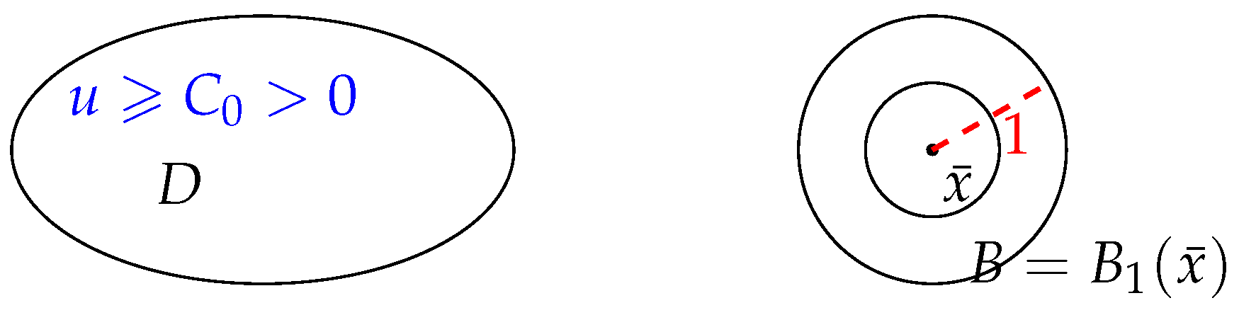
For a nonnegative super s-harmonic function, if it assumes positive values in some region D, then this “positiveness” will be “diffused”, or be “averaged out”, to any other region B, as illustrated in the figure below. This “averaging effect” depends on the distance between the two regions: the closer the distance, the greater the effect.

More precisely, we have

Theorem 1. 

Let D be a region in ${\mathbb{R}}^n$ and assume that

$$u\left(x\right)⩾c_0>0,x\in D.$$

(5)

Suppose that

$${(-\Delta )}^{s}u\left(x\right)⩾0in{B}_1\left(\overline{x}\right),andu\left(x\right)⩾0in{B}_1^c\left(\overline{x}\right),$$

for any point $\overline{x}$ such that $B_1\left(\overline{x}\right)$ is disjointed from D as shown in Figure 1. Then there exists a constant $c_1>0$ depending on $C_0$ and the distance between $\overline{x}$ and D, such that

$$u\left(\overline{x}\right)⩾c_1.$$

The key distinction between the averaging effect of the fractional Laplacian and the average inequality for the classical Laplacian lies in the non-locality of the former. In the fractional case, it suffices to assume that u is s-superharmonic only in $B_1\left(\overline{x}\right)$. Indeed, for $x\in B_1\left(\overline{x}\right)$, the inequality

$${(-\Delta )}^{s}u\left(x\right)\equiv C_{n,s}PV{\int }_{{\mathbb{R}}^n}{\displaystyle \frac{u\left(x\right)-u\left(y\right)}{{|x-y|}^{n+2s}}}dy\ge 0,$$

shows that the values of u outside $B_1\left(\overline{x}\right)$—in particular, in any other region D—influence the behavior of u in $B_1\left(\overline{x}\right)$, since the integral involves all points in ${\mathbb{R}}^n$.

However, for local operators including the classical Laplacian, it is not enough to assume that u is super-harmonic only in $B_1\left(\overline{x}\right)$. In order for the classical mean-value inequality to hold, u is required to be super-harmonic in a large ball $B_R\left(\overline{x}\right)$ containing both D and $B_1\left(\overline{x}\right)$. Here is a counter example:

Let u be a nonnegative continuous function defined by

$$u\left(x\right)=\left\{\begin{array}{cc}0,\hfill & x\in B_1\left(\overline{x}\right),\hfill \\ 1,\hfill & x\in D.\hfill \end{array}\right.$$

Then obviously, u satisfies all the conditions in the theorem:

$$-\Delta u\left(x\right)=0,x\in B_1\left(\overline{x}\right);u\left(x\right)\ge 0,x\in B_1^c\left(\overline{x}\right);u\left(x\right)\ge c_o>0,x\in D.$$

However, the conclusion of the theorem is no longer valid. This demonstrates that the positivity of u in D does not influence its values in $B_1\left(\overline{x}\right)$ in the case of the classical Laplacian.

If we strengthen the condition, that is to require u be super-harmonic in a sufficiently large ball containing D and $B_1\left(\overline{x}\right)$:

$$-\Delta u\left(x\right)\ge 0,x\in B_R\left(\overline{x}\right)\mathrm{with}D\subset B_R\left(\overline{x}\right),$$

then by (4), we can arrive at the conclusion of the theorem.

• Idea of the proof of the theorem

We try to find a sub-solution $\underline{u}$ in $B_1\left(\overline{x}\right)$ that is positively bounded away from 0.

To be a sub-solution, we require

$${(-\Delta )}^s\underline{u}\left(x\right)⩽{(-\Delta )}^{s}u\left(x\right),x\in B_1\left(\overline{x}\right),$$

and

$$\underline{u}\left(x\right)\le u\left(x\right),x\in B_1^c\left(\overline{x}\right).$$

These can be achieved by ${\chi }_D\left(x\right)u\left(x\right)$. As one will see by direct computation in the following proof, ${(-\Delta )}^s\left[{\chi }_D\left(x\right)u\left(x\right)\right]$ is negative, and negatively bounded away from zero if the point x is within a certain distance from D.

In order for the sub-solution to be positively bounded away from 0 in $B_1\left(\overline{x}\right)$, we need to add a function $\phi \left(x\right)$, that is we select

$$\underline{u}\left(x\right):={\chi }_D\left(x\right)u\left(x\right)+\epsilon \phi \left(x\right)$$

by a proper choice of $\phi \left(x\right)$. For a sufficiently small $\epsilon$, the negativeness of ${(-\Delta )}^s\left[{\chi }_D\left(x\right)u\left(x\right)\right]$ would overcome $ϵ{(-\Delta )}^s\phi$, and thus render ${(-\Delta )}^s\underline{u}\left(x\right)\le 0$.

This is a frequently used technique in fractional analysis.

Proof. 

Let

$$\phi \left(x\right):=a(1-|x-\overline{x}{{|}^2)}_{+}^s.$$

Then, it is known that by a proper choice of positive number a

$$\left\{\begin{array}{cc}{(-\Delta )}^s\phi \left(x\right)=1,\hfill & x\in B_1\left(\overline{x}\right)\hfill \\ \phi \left(x\right)=0,\hfill & x\in B_1^c\left(\overline{x}\right).\hfill \end{array}\right.$$

Let

$${\chi }_D\left(x\right):=\left\{\begin{array}{cc}1,\hfill & x\in D,\hfill \\ 0,\hfill & x\notin D,\hfill \end{array}\right.$$

be the characteristic function of set D.

Denote

$$\underline{u}\left(x\right):={\chi }_D\left(x\right)u\left(x\right)+\epsilon \phi \left(x\right).$$

For $x\in B_1\left(\overline{x}\right)$, by (5) we calculate

$$\begin{array}{ccc}\hfill {(-\Delta )}^s\underline{u}\left(x\right)& =& {(-\Delta )}^s\left({\chi }_D\left(x\right)u\left(x\right)\right)+\epsilon \hfill \\ & =& C_{n,s}P.V.{\int }_{{\mathbb{R}}^n}{\displaystyle \frac{0-{\chi }_D\left(y\right)u\left(y\right)}{{|x-y|}^{n+2s}}}dy+\epsilon \hfill \\ & =& C_{n,s}{\int }_D{\displaystyle \frac{-u\left(y\right)}{{|x-y|}^{n+2s}}}dy+\epsilon \hfill \\ & ⩽& -C_{n,s}{c}_0{\int }_D{\displaystyle \frac{1}{{|x-y|}^{n+2s}}}dy+\epsilon \hfill \\ & ⩽& -C_2+\epsilon .\hfill \end{array}$$

Choosing $\epsilon =C_2$, we obtain

$${(-\Delta )}^s\underline{u}\left(x\right)⩽0,x\in B_1\left(\overline{x}\right).$$

This verifies the inequality for $\underline{u}$ to be a sub-solution.

To check the exterior condition, we use the condition

$$u\left(x\right)⩾0,x\notin B_1\left(\overline{x}\right)$$

to derive

$$\underline{u}\left(x\right)={\chi }_D\left(x\right)u\left(x\right)⩽u\left(x\right).$$

Therefore, $\underline{u}$ is a sub-solution in $B_1\left(\overline{x}\right)$, satisfying

$$\left\{\begin{array}{cc}{(-\Delta )}^s\underline{u}\left(x\right)⩽{(-\Delta )}^{s}u\left(x\right),\hfill & x\in B_1\left(\overline{x}\right),\hfill \\ \underline{u}\left(x\right)⩽u\left(x\right).\hfill & x\notin B_1\left(\overline{x}\right).\hfill \end{array}\right.$$

Then by the maximum principle, we derive

$$u\left(x\right)⩾\underline{u}\left(x\right),x\in B_1\left(\overline{x}\right),$$

and consequently,

$$u\left(x\right)⩾\epsilon \phi \left(x\right),x\in B_1\left(\overline{x}\right).$$

Hence, we conclude that

$$u\left(\overline{x}\right)⩾\epsilon >0.$$

The choice of $\epsilon$ indicates that the closer the distance between the ball $B_1\left(\overline{x}\right)$ and the region D, the larger the positive constant $c_1$ can be. □

Remark 1. 

Actually, the condition

$${(-\Delta )}^{s}u\left(x\right)⩾0in{B}_1\left(\overline{x}\right)$$

can be replaced by a weaker assumption

$${(-\Delta )}^{s}u\left(x\right)⩾-\delta in{B}_1\left(\overline{x}\right)$$

for some small $\delta >0$ (see [29]), or even a weaker one

$${(-\Delta )}^{s}u\left(x\right)⩾f\left(u\left(x\right)\right)in{B}_1\left(\overline{x}\right)$$

with $f\left(0\right)\ge 0$ (see [47]).

Under these weaker conditions, the averaging effect can be applied to much more general situations.

2.1.2. Under Weaker Conditions

Here is the averaging effect under weaker conditions.

Theorem 2. 

Let D be a region in ${\mathbb{R}}^n$ and assume that

$$u\left(x\right)⩾c_0>0,x\in D.$$

(6)

Suppose that

$${(-\Delta )}^{s}u\left(x\right)⩾-\delta in{B}_1\left(\overline{x}\right)$$

for some sufficiently small $\delta >0$ depending on the distance between D and $B_1\left(\overline{x}\right)$; and

$$u\left(x\right)⩾0in{B}_1^c\left(\overline{x}\right),$$

for any $\overline{x}$ such that $B_1\left(\overline{x}\right)$ is disjointed from D. Then there exists a constant $c_1>0$ depending on $c_0$ and the distance between $\overline{x}$ and D, such that

$$u\left(\overline{x}\right)⩾c_1.$$

Proof. 

The proof is quite similar to that of Theorem 1, except the choice of $\epsilon$. This time, we choose $\epsilon ={\displaystyle \frac{C_2}{2}}$. Then for $\delta ={\displaystyle \frac{C_2}{2}}$, we still have

$${(-\Delta )}^s\underline{u}\left(x\right)⩽{(-\Delta )}^{s}u\left(x\right),x\in B_1\left(\overline{x}\right).$$

Then the rest of the proof goes the same way as in the proof of Theorem 1. □

When u is uniformly continuous, positivity at a single point $x^0$ implies positivity in a neighborhood of that point. That is, if $u\left(x^0\right)>0$, then there exists a neighborhood D of $x^0$ such that u is bounded away from zero in D. Using this observation, we may reformulate the averaging effect in a form that is more convenient for application.

Corollary 1. 

Suppose u is uniformly continuous, nonnegative, and at some point $x^0$,

$$u\left(x^0\right)=c_0>0.$$

Assume that

$${(-\Delta )}^{s}u\left(x\right)⩾-\delta inaneighborhoodofanotherpoint\overline{x}$$

for some sufficiently small $\delta >0$.

Then there exists a constant $c_1>0$ depending on $c_0$ and the distance between $x^0$ and $\overline{x}$, such that

$$u\left(\overline{x}\right)⩾c_1.$$

Theorem 3 

([47]). Let D be a region in ${\mathbb{R}}^n$ and assume that

$$u\left(x\right)⩾c_0>0,x\in D.$$

(7)

Let $\overline{x}$ be any point not in D and $\delta >0$ such that $B_{\delta }\left(\overline{x}\right)$ is disjointed from D.

Suppose that

$${(-\Delta )}^{s}u\left(x\right)⩾f\left(u\left(x\right)\right)in{B}_{\delta }\left(\overline{x}\right)$$

(8)

with $f\left(0\right)\ge 0$. Assume

$$u\left(x\right)⩾0in{B}_{\delta }^c\left(\overline{x}\right).$$

Then there exists a constant ${ϵ}_0>0$ depending only on $c_0$, the distance between $\overline{x}$ and D, and the uniform continuity of u and the continuity of f near 0, such that

$$u\left(\overline{x}\right)⩾{ϵ}_0.$$

Remark 2. 

It is important that this ${ϵ}_0$ does not depend on the location of D. In applications, such set D may move toward infinity. This is the essential difference between the averaging effect and the strong maximum principle.

Proof. 

From the previous proof, we have derived that there exists $c_1>0$, such that

$${(-\Delta )}^s\left[{\chi }_D\left(x\right)u\left(x\right)\right]\le -2c_1.$$

(9)

Let

$$\underline{u}\left(x\right):={\chi }_D\left(x\right)u\left(x\right)+c_1{\psi }_{\delta }\left(x\right),$$

where

$${\psi }_{\delta }\left(x\right):=a({\delta }^2-|x-\overline{x}{{|}^2)}_{+}^s.$$

Then, it is known that by a proper choice of positive number a

$$\left\{\begin{array}{cc}{(-\Delta )}^s{\psi }_{\delta }\left(x\right)=1,\hfill & x\in B_{\delta }\left(\overline{x}\right)\hfill \\ {\psi }_{\delta }\left(x\right)=0,\hfill & x\in B_{\delta }^c\left(\overline{x}\right).\hfill \end{array}\right.$$

Consequently,

$${(-\Delta )}^s\underline{u}\left(x\right)\le -c_1.$$

(10)

In order to make $\underline{u}\left(x\right)$ a sub-solution, it suffices that

$$f\left(u\left(x\right)\right)\ge -c_1,\forall x\in B_{\delta }\left(\overline{x}\right).$$

(11)

Due to the condition $f\left(0\right)\ge 0$, we only need to ensure

$$|f\left(u\left(x\right)\right)-f\left(0\right)|\le c_1,\forall x\in B_{\delta }\left(\overline{x}\right).$$

(12)

In fact, on one hand, by the uniform continuity of u and the continuity of f, there is a ${\delta }_1>0$, such that

$$|f\left(u\left(x\right)\right)-f\left(u\left(\overline{x}\right)\right)|\le {\displaystyle \frac{c_1}{2}},\forall x\in B_{{\delta }_1}\left(\overline{x}\right).$$

(13)

We now take $\delta$ as ${\delta }_1$.

On the other hand, by the continuity of f near 0, there exists ${\delta }_2>0$, such that

$$|f\left(0\right)-f\left(u\left(\overline{x}\right)\right)|\le {\displaystyle \frac{c_1}{2}},\mathrm{whenever}u\left(\overline{x}\right)\le {\delta }_2.$$

(14)

By (11)–(14), whenever $u\left(\overline{x}\right)\le {\delta }_2$, $\underline{u}\left(x\right)$ is a sub-solution in $B_{{\delta }_1}\left(\overline{x}\right)$, and it follows that

$$u\left(\overline{x}\right)\ge \underline{u}\left(\overline{x}\right)=c_1{\psi }_{{\delta }_1}\left(\overline{x}\right)=c_{1}a{\delta }_1^{2s}.$$

(15)

We conclude that

$$u\left(\overline{x}\right)\ge min\{c_{1}a{\delta }_1^{2s},{\delta }_2\}:={ϵ}_0.$$

In fact, if

$$u\left(\overline{x}\right)\ge {\delta }_2,$$

we are done, while if

$$u\left(\overline{x}\right)<{\delta }_2,$$

then by (15), we have

$$u\left(\overline{x}\right)\ge c_{1}a{\delta }_1^{2s}.$$

In either case, we must have

$$u\left(\overline{x}\right)\ge {ϵ}_0.$$

This completes the proof. □

2.2. Averaging Effect for the Fractional Parabolic Operators

The averaging effect is also valid for fractional parabolic operators, such as ${\partial }_t+{(-\Delta )}^s$ and ${\partial }_t^{\alpha }+{(-\Delta )}^s$, where ${\partial }_t^{\alpha }$ is known as the Marchaud fractional derivative defined as

$${\partial }_t^{\alpha }u\left(t\right)=C_{\alpha }{\int }_{-\infty }^t{\displaystyle \frac{u\left(t\right)-u\left(\tau \right)}{{(t-\tau )}^{1+\alpha }}}d\tau$$

for $0<\alpha <1$. Take ${\partial }_t+{(-\Delta )}^s$ for example, we have

Theorem 4 

(Averaging effects). Let D be a region in ${\mathbb{R}}^n$ and $t_0\in \mathbb{R}$ be a real number. For any $x^0\in {\mathbb{R}}^n$, if there exists a positive radius $r>0$ such that $B_r\left(x^0\right)\cap \overline{D}=⌀$, and

$$u(x,t)\ge C_0>0inD\times (t_0-r^{2s},t_0+r^{2s}].$$

(16)

Assume that

$$u(x,t)\in \left(C_{\mathrm{loc}}^{1,1}\left(B_r\left(x^0\right)\right)\cap {\mathcal{L}}_{2s}\left({\mathbb{R}}^n\right)\right)\times C^1\left([t_0-r^{2s},t_0+r^{2s}]\right)$$

is lower semi-continuous in x on $\overline{B_r\left(x^0\right)}$, satisfying

$$\left\{\begin{array}{cc}{\partial }_{t}u(x,t)+{(-\Delta )}^{s}u(x,t)\ge -\delta ,\hfill & (x,t)\in B_r\left(x^0\right)\times (t_0-r^{2s},t_0+r^{2s}],\hfill \\ u(x,t)\ge 0,\hfill & (x,t)\in B_r^c\left(x^0\right)\times (t_0-r^{2s},t_0+r^{2s}],\hfill \\ u(x,t_0-r^{2s})\ge 0,\hfill & x\in B_r\left(x^0\right),\hfill \end{array}\right.$$

(17)

for some sufficiently small $\delta >0$. Then there exists a positive constant

$$C_1=C_1\left(\alpha ,n,s,C_0,diam\left(D\right),dist(x^0,D)\right)$$

such that

$$u(x^0,t_0)\ge C_1>0,$$

where $diam\left(D\right)$ represents the diameter of region D, and $dist(x^0,D)$ denotes the distance from point $x^0$ to region D.

For the corresponding theorem on the dual fractional parabolic operator ${\partial }_t^{\alpha }+{(-\Delta )}^s$, please see [48].

Proof of Theorem 4. 

The overall approach is again by employing a sub-solution, which is similar to the proof for Theorem 1. However, in this process, we need to take the time variable t into consideration. To this end, we choose the sub-solution as

$$\underline{u}(x,t):=u(x,t){\chi }_D\left(x\right)+ϵ\psi (x,t),$$

where $ϵ$ is a positive constant to be determined later, and ${\chi }_D$ is the characteristic function on D, and

$$\psi (x,t):=\varphi \left(x\right)\eta \left(t\right):=C{\left(1-{\left|{\displaystyle \frac{x-x^0}{r}}\right|}^2\right)}_{+}^s\eta \left(t\right).$$

Here $\eta \left(t\right)$ is a smooth cut-off function with compact support in $(t_0-r^{2s},t_0+r^{2s})$, satisfying

$$0\le \eta \left(t\right)\le 1,\mathrm{and}\eta \left(t\right)\equiv 1\mathrm{in}[t_0-{\displaystyle \frac{r^{2s}}{2}},t_0+{\displaystyle \frac{r^{2s}}{2}}].$$

It is well known that, by a proper choice of positive constant C, we can make

$${(-\Delta )}^s\varphi \left(x\right)={\displaystyle \frac{1}{r^{2s}}}\mathrm{in}{B}_r\left(x^0\right),$$

(18)

while obviously, $\varphi \left(x\right)\equiv 0$ in $B_r^c\left(x^0\right)$.

We verify that $\underline{u}(x,t)$ is a sub-solution in $B_r\left(x^0\right)\times (t_0-r^{2s},t_0+r^{2s}]$. In fact, by (16)–(18) and taking into account $B_r\left(x^0\right)\cap \overline{D}=⌀$ and the smoothness of $\eta \left(t\right)$, we derive, for $(x,t)\in B_r\left(x^0\right)\times (t_0-r^{2s},t_0+r^{2s}]$,

$$\begin{array}{ccc}& & {\partial }_t\left(u(x,t)-\underline{u}(x,t)\right)+{(-\Delta )}^s\left(u(x,t)-\underline{u}(x,t)\right)\hfill \\ & \ge & -\delta -ϵ\varphi \left(x\right){\partial }_t\eta \left(t\right)-{(-\Delta )}^s\left(u(x,t){\chi }_D\left(x\right)\right)-ϵ\eta \left(t\right){(-\Delta )}^s\varphi \left(x\right)\hfill \\ & \ge & -\delta +C_{n,s}{C}_0{\int }_D{\displaystyle \frac{1}{{|x-y|}^{n+2s}}}dy-{\displaystyle \frac{Cϵ}{r^{2s}}}\hfill \\ & \ge & -\delta +C_2-{\displaystyle \frac{Cϵ}{r^{2s}}}.\hfill \end{array}$$

Now choosing $\delta ={\displaystyle \frac{C_2}{2}}$ and $ϵ={\displaystyle \frac{C_2{r}^{2s}}{2C}}$, we arrive at the desired differential inequality for a sub-solution

$$[{\partial }_t+{(-\Delta )}^s]\left(u(x,t)-\underline{u}(x,t)\right)\ge 0,(x,t)\in B_r\left(x^0\right)\times (t_0-r^{2s},t_0+r^{2s}].$$

To verify the exterior condition, we have, for

$$(x,t)\in B_r^c\left(x^0\right)\times (t_0-r^{2s},t_0+r^{2s}],$$

it holds

$$u(x,t)-\underline{u}(x,t)=u(x,t)-u(x,t){\chi }_D\left(x\right)\ge 0,$$

which is ensured by the definition of $\psi (x,t)$ and the exterior condition in (17).

To see the initial condition, we notice that $\underline{u}(x,t_0-r^{2s})=0$ for $x\in B_r\left(x^0\right)$ since both ${\chi }_D\left(x\right)$ and $\eta \left(t\right)$ vanish here.

In summary, we have obtained

$$\left\{\begin{array}{cc}[{\partial }_t+{(-\Delta )}^s]\left(u(x,t)-\underline{u}(x,t)\right)\ge 0,\hfill & \mathrm{in}{B}_r\left(x^0\right)\times (t_0-r^{2s},t_0+r^{2s}],\hfill \\ u(x,t)-\underline{u}(x,t)\ge 0,\hfill & \mathrm{in}{B}_r^c\left(x^0\right)\times (t_0-r^{2s},t_0+r^{2s}],\hfill \\ u(x,t)-\underline{u}(x,t)\ge 0,\hfill & \mathrm{in}{B}_r\left(x^0\right)\times \{t_0-r^{2s}\}.\hfill \end{array}\right.$$

Then the maximum principle implies that

$$u(x,t)\ge \underline{u}(x,t)for(x,t)\in B_r\left(x^0\right)\times (t_0-r^{2s},t_0+r^{2s}].$$

Finally, it follows that

$$u(x^0,t_0)\ge \underline{u}(x^0,t_0)=ϵ\varphi \left(x^0\right)\eta \left(t_0\right)=Cϵ=C_1>0.$$

This completes the proof of Theorem 4. □

In the case when the function is uniformly continuous, we have a similar corollary as in the elliptic case.

Corollary 2. 

Suppose $u(x,t)$ is uniformly continuous in both x and t, nonnegative, and at some point $(x^0,t_0)$,

$$u(x^0,t_0)⩾c_0>0.$$

Assume that

$${\partial }_{t}u+{(-\Delta )}^{s}u(x,t)⩾-\delta inaparabolicneighborhoodofanotherpoint(\overline{x},t_0)$$

for some sufficiently small $\delta >0$.

Then there exists a constant $c_1>0$ depending on $c_0$ and the distance between $x^0$ and $\overline{x}$, such that

$$u(\overline{x},t_0)⩾c_1.$$

2.3. Averaging Effect for Antisymmetric Functions

When employing the method of moving planes, what we consider are antisymmetric functions.

As usual, let

$$T_{\lambda }=\{x\in {\mathbb{R}}^n\mid x_1=\lambda ,\mathrm{for}\mathrm{some}\lambda \in \mathbb{R}\}.$$

Let

$$x^{\lambda }=(2\lambda -x_1,x_2,\dots ,x_n)$$

be the reflection of x about the plane $T_{\lambda }$. Denote

$${\Sigma }_{\lambda }=\{x\in {\mathbb{R}}^n\mid x_1<\lambda \}.$$

Theorem 5 

([34] Averaging effects for antisymmetric functions—the elliptic case). Let D be a region in ${\Sigma }_{\lambda }$. For any given point $x^0\in {\Sigma }_{\lambda }$, if there exists a ball $B_r\left(x^0\right)\subset {\Sigma }_{\lambda }$ such that $B_r\left(x^0\right)\cap \overline{D}=⌀$ and

$$w\left(x\right)\ge c_0>0inD.$$

(19)

Assume that

$$w\left(x\right)\in \left(C_{\mathrm{loc}}^{1,1}\left(B_r\left(x^0\right)\right)\cap {\mathcal{L}}_{2s}\left({\mathbb{R}}^n\right)\right)$$

is lower semi-continuous on $\overline{B_r\left(x^0\right)}$ and satisfies

$$\left\{\begin{array}{cc}{(-\Delta )}^{s}w\left(x\right)\ge -\delta ,\hfill & x\in B_r\left(x^0\right),\hfill \\ w\left(x\right)\ge 0,\hfill & x\in \left({\Sigma }_{\lambda }\setminus B_r\left(x^0\right)\right),\hfill \\ w\left(x\right)=-w\left(x^{\lambda }\right),\hfill & x\in {\Sigma }_{\lambda },\hfill \end{array}\right.$$

(20)

for some sufficiently small $\delta >0$. Then there exists a positive constant $c_1$ depending on $c_0$, $diam\left(D\right)$, $dist(x^0,D)$, $dist(\partial D,T_{\lambda })$, and $dist(x^0,T_{\lambda })$, such that

$$w\left(x^0\right)\ge c_1>0,$$

where $dist(\partial D,T_{\lambda })$ stands for the distance between the boundary $\partial D$ and the hyperplane $T_{\lambda }$.

The proof of this theorem is similar (and simpler) to that of the following parabolic version, we skip it here.

Theorem 6 

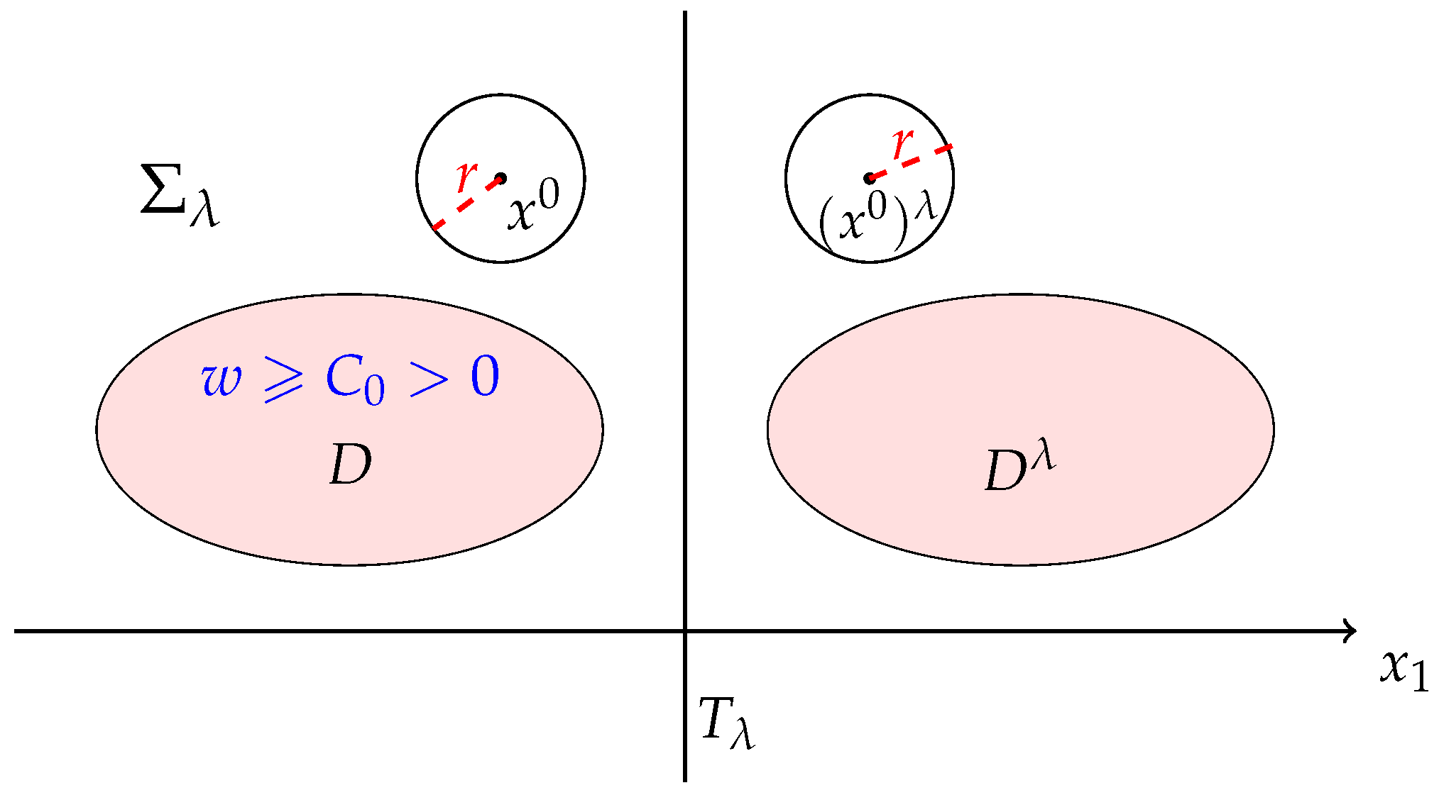
([48] Averaging effects for antisymmetric functions—the parabolic case). Let $D\subset {\Sigma }_{\lambda }$ be a region and $t_0\in \mathbb{R}$ be a real number. For any $x^0\in {\Sigma }_{\lambda }$, if there exists a ball $B_r\left(x^0\right)\subset {\Sigma }_{\lambda }$ such that $B_r\left(x^0\right)\cap \overline{D}=⌀$ as shown in Figure 2, and

$$w(x,t)\ge c_0>0inD\times (t_0-r^{2s},t_0+r^{2s}].$$

(21)

Assume that

$$w(x,t)\in \left(C_{\mathrm{loc}}^{1,1}\left(B_r\left(x^0\right)\right)\cap {\mathcal{L}}_{2s}\left({\mathbb{R}}^n\right)\right)\times \left(C^1\left([t_0-r^{2s},t_0+r^{2s}]\right)\right)$$

is lower semi-continuous in x on $\overline{B_r\left(x^0\right)}$, satisfying

$$\left\{\begin{array}{cc}{\partial }_{t}w(x,t)+{(-\Delta )}^{s}w(x,t)\ge -\delta ,\hfill & (x,t)\in B_r\left(x^0\right)\times (t_0-r^{2s},t_0+r^{2s}],\hfill \\ w(x,t)\ge 0,\hfill & (x,t)\in \left({\Sigma }_{\lambda }\setminus B_r\left(x^0\right)\right)\times (t_0-r^{2s},t_0+r^{2s}],\hfill \\ w(x,t^0)\ge 0,\hfill & x\in B_r\left(x^0\right),\hfill \\ w(x,t)=-w(x^{\lambda },t),\hfill & (x,t)\in {\Sigma }_{\lambda }\times \mathbb{R},\hfill \end{array}\right.$$

(22)

for some sufficiently small $\delta >0$. Then there exists a positive constant $c_1$ depending on $c_0$, $diam\left(D\right)$, $dist(x^0,D)$, $dist(\partial D,T_{\lambda })$, and $dist(x^0,T_{\lambda })$, such that

$$w(x^0,t_0)\ge c_1>0,$$

where $dist(\partial D,T_{\lambda })$ stands for the distance between the boundary $\partial D$ and the hyperplane $T_{\lambda }$.

Proof. 

The key element in this proof is the construction of an antisymmetric sub-solution for $w(x,t)$. Let

$$\varphi \left(x\right):={\left(1-{\left|{\displaystyle \frac{x-x^0}{r}}\right|}^2\right)}_{+}^s\mathrm{and}{\varphi }_{\lambda }\left(x\right):={\left(1-{\left|{\displaystyle \frac{x^{\lambda }-x^0}{r}}\right|}^2\right)}_{+}^s,$$

then it is obvious that

$$\Phi \left(x\right):=\varphi \left(x\right)-{\varphi }_{\lambda }\left(x\right)$$

is an antisymmetric function with respect to the plane $T_{\lambda }$. Denote

$$\eta \left(t\right)\in C_0^{\infty }\left((t_0-r^{2s},t_0+r^{2s})\right)$$

which is a smooth cut-off function valued between 0 and 1, satisfying

$$\eta \left(t\right)\equiv 1\mathrm{in}[t_0-{\displaystyle \frac{r^{2s}}{2}},t_0+{\displaystyle \frac{r^{2s}}{2}}].$$

Let $D^{\lambda }$ be the reflection of D with respect to the plane $T_{\lambda }$ as illustrated in Figure 2 below, and

$$\underline{w}(x,t)=w(x,t){\chi }_{D\cup D^{\lambda }}\left(x\right)+ϵ\Phi \left(x\right)\eta \left(t\right),$$

where $ϵ$ is a positive constant to be determined later, and ${\chi }_{D\cup D^{\lambda }}\left(x\right)$ is the characteristic function in the region $D\cup D^{\lambda }$.

Next we show that the antisymmetric function $\underline{w}(x,t)$ is a sub-solution for $w(x,t)$ in $B_r\left(x^0\right)\times (t_0-r^{2s},t_0+r^{2s}]$.

We first verify the differential inequality in this region. By a straightforward calculation, we derive

$$\begin{array}{ccc}& & {\partial }_t\left(w(x,t)-\underline{w}(x,t)\right)+{(-\Delta )}^s\left(w(x,t)-\underline{w}(x,t)\right)\hfill \\ & \ge & -\delta -ϵ\Phi \left(x\right){\partial }_t^{\alpha }\eta \left(t\right)-{(-\Delta )}^s\left(w(x,t){\chi }_{D\cup D^{\lambda }}\left(x\right)\right)-ϵ\eta \left(t\right){(-\Delta )}^s\left(\varphi \left(x\right)-{\varphi }_{\lambda }\left(x\right)\right)\hfill \\ & \ge & -\delta +C_{n,s}{\int }_{D\cup D^{\lambda }}{\displaystyle \frac{w(y,t)}{{|x-y|}^{n+2s}}}dy-{\displaystyle \frac{Cϵ}{r^{2s}}}-C_{n,s}ϵ{\int }_{B_r\left({\left(x^0\right)}^{\lambda }\right)}{\displaystyle \frac{1}{{|x-y|}^{n+2s}}}dy\hfill \\ & \ge & -\delta +C_{n,s}{c}_0{\int }_D\left[{\displaystyle \frac{1}{{|x-y|}^{n+2s}}}-{\displaystyle \frac{1}{|x-y^{\lambda }{|}^{n+2s}}}\right]dy-{\displaystyle \frac{Cϵ}{r^{2s}}}\hfill \\ & \ge & -\delta +C_2-{\displaystyle \frac{Cϵ}{r^{2s}}}\ge 0.\hfill \end{array}$$

Here we have selected $\delta ={\displaystyle \frac{C_2}{2}}$ and $ϵ={\displaystyle \frac{C_2{r}^{2s}}{2C}}$.

For $(x,t)\in ({\Sigma }_{\lambda }\setminus B_r\left(x^0\right))\times (t_0-r^{2s},t_0+r^{2s}]$, it follows from the exterior condition in (22) that

$$w(x,t)-\underline{w}(x,t)=w(x,t)-w(x,t){\chi }_{D\cup D^{\lambda }}\left(x\right)\ge 0.$$

Finally, we apply the initial condition in (22) to derive

$$w(x,t^0)-\underline{w}(x,t^0)=w(x,t^0)\ge 0,\forall x\in B_r\left(x^0\right).$$

Let $W(x,t)=w(x,t)-\underline{w}(x,t)$. In summary, we have deduced that

$$\left\{\begin{array}{cc}[{\partial }_t+{(-\Delta )}^s]W(x,t)\ge 0,\hfill & \mathrm{in}{B}_r\left(x^0\right)\times (t_0-r^{2s},t_0+r^{2s}],\hfill \\ W(x,t)\ge 0,\hfill & \mathrm{in}({\Sigma }_{\lambda }\setminus B_r\left(x^0\right))\times (t_0-r^{2s},t_0+r^{2s}],\hfill \\ W(x,t)\ge 0,\hfill & \mathrm{in}{B}_r\left(x^0\right)\times \left\{t^0\right\},\hfill \\ W(x,t)=-W(x^{\lambda },t),\hfill & \mathrm{in}{\Sigma }_{\lambda }\times \mathbb{R}.\hfill \end{array}\right.$$

Then applying the maximum principle for antisymmetric functions, we obtain

$$W(x,t)\ge 0\mathrm{in}{B}_r\left(x^0\right)\times (t_0-r^{2s},t_0+r^{2s}].$$

(23)

Otherwise, there exists $(\overline{x},\overline{t})\in B_r\left(x^0\right)\times (t_0-r^{2s},t_0+r^{2s}]$, such that

$$W(\overline{x},\overline{t})=\underset{B_r\left(x^0\right)\times (t_0-r^{2s},t_0+r^{2s}]}{min}W(x,t)<0.$$

If this negative minimum $(\overline{x},\overline{t})$ is attained in the interior of the cylinder

$$B_r\left(x^0\right)\times (t_0-r^{2s},t_0+r^{2s}],$$

then we have

$${\partial }_{t}W(\overline{x},\overline{t})=0,\mathrm{and}{(-\Delta )}^{s}W(\overline{x},\overline{t})<0$$

which is a contradiction with

$$[{\partial }_t+{(-\Delta )}^s]W(x,t)\ge 0,\mathrm{in}{B}_r\left(x^0\right)\times (t_0-r^{2s},t_0+r^{2s}].$$

(24)

If this minimum $(\overline{x},\overline{t})$ is attained at the top of the cylinder

$$B_r\left(x^0\right)\times (t_0-r^{2s},t_0+r^{2s}]$$

with $\overline{t}=t_0+r^{2s}$, then we have

$${\partial }_{t}W(\overline{x},\overline{t})\le 0,\mathrm{and}{(-\Delta )}^{s}W(\overline{x},\overline{t})<0,$$

again a contradiction with (24). Therefore, (24) must be valid.

In particular

$$w(x^0,t_0)\ge \underline{w}(x^0,t_0)=ϵ\varphi \left(x^0\right)\eta \left(t_0\right)=ϵ=:c_1>0.$$

This completes the proof of the theorem. □

3. Applications of the Averaging Effects

3.1. Radial Symmetry in a Unit Ball

In this section, we will use a simple example—deriving the radial symmetry of positive solutions on a unit ball—to illustrate the applications of the averaging effect.

Consider entire solutions to the fractional parabolic problem

$$\left\{\begin{array}{cc}{\displaystyle \frac{\partial u}{\partial t}}+{(-\Delta )}^{s}u=f\left(u(x,t)\right),u>0,\hfill & (x,t)\in B_1\left(0\right)\times \mathbb{R},\hfill \\ u(x,t)\equiv 0,\hfill & (x,t)\in B_1^c\left(0\right)\times \mathbb{R}.\hfill \end{array}\right.$$

(25)

Theorem 7. 

Let $u(x,t)$ be a classical solution of (25). Assume that $f(·)$ is Lipschitz continuous,

$$f\left(0\right)\ge 0and{f}^{\prime }\left(0\right)\le 0.$$

Then for each fixed t, $u(x,t)$ is radially symmetric and strictly decreasing in $\left|x\right|$ about the origin.

Proof. 

As usual, we will apply the method of moving planes to derive the radial symmetry. To this end, we choose $x_1$-axis to be in any given direction and let $T_{\lambda }$, ${\Sigma }_{\lambda }$, and $x^{\lambda }$ as previously defined. For each t, let

$$w_{\lambda }(x,t):=u_{\lambda }(x,t)-u(x,t)$$

with $u_{\lambda }(x,t)=u(x^{\lambda },t)$. Denote

$${\mathsf{\Omega }}_{\lambda }:={\Sigma }_{\lambda }\cap B_1\left(0\right),\lambda \le 0.$$

Then

$$\left\{\begin{array}{cc}{\displaystyle \frac{\partial w_{\lambda }(x,t)}{\partial t}}+{(-\Delta )}^s{w}_{\lambda }(x,t)=c_{\lambda }(x,t)w_{\lambda }(x,t),\hfill & (x,t)\in {\mathsf{\Omega }}_{\lambda }\times \mathbb{R},\hfill \\ w_{\lambda }(x,t)\ge 0,\hfill & (x,t)\in ({\Sigma }_{\lambda }\setminus {\mathsf{\Omega }}_{\lambda })\times \mathbb{R},\hfill \end{array}\right.$$

(26)

where $c_{\lambda }(x,t)=f^{\prime }\left({\xi }_{\lambda }(x,t)\right)$ with ${\xi }_{\lambda }(x,t)$ is valued between $u(x,t)$ and $u_{\lambda }(x,t)$.

There are generally two steps.

In Step 1, we show that for $\lambda >-1$ and sufficiently close to $-1$, it holds

$$w_{\lambda }(x,t)\ge 0,\forall (x,t)\in {\mathsf{\Omega }}_{\lambda }\times \mathbb{R}.$$

(27)

This provides a starting point to move the plane $T_{\lambda }$.

Then in Step 2, we move the plane $T_{\lambda }$ continuously to the right as long as Inequality (27) holds to its limiting position. We prove that this position must be $T_0$, the plane passing through the origin. Since $x_1$-direction can be chosen arbitrarily, we conclude that u must be radially symmetric and monotone decreasing about the origin. Here the averaging effect will come into play.

Now, we carry out the details.

• Step 1.

We show that

$$w_{\lambda }(x,t)⩾0,(x,t)\in {\mathsf{\Omega }}_{\lambda }\times \mathbb{R}$$

(28)

for $\lambda >-1$ and sufficiently close to $-1$.

We deduce (28) again by a contradiction argument. Suppose otherwise,

$$\underset{{\mathsf{\Omega }}_{\lambda }\times \mathbb{R}}{inf}{w}_{\lambda }=-m<0.$$

Unlike the elliptic case where ${\mathsf{\Omega }}_{\lambda }$ is a bounded domain, here ${\mathsf{\Omega }}_{\lambda }\times \mathbb{R}$ is an infinite cylinder and the infimum of $w_{\lambda }$ may not be attained.

For each fixed t, since ${\mathsf{\Omega }}_{\lambda }$ is bounded, $w_{\lambda }(x,t)$ can attain its minimum at some point $x^0\in {\mathsf{\Omega }}_{\lambda }$, and similar to the elliptic case, we still have the crucial inequality as stated in the following lemma.

Lemma 1. 

For each fixed $t\in \mathbb{R}$, assume that the antisymmetric function $w_{\lambda }(·,t)\in {\mathcal{L}}_{2s}\cap C_{loc}^{1,1}\left({\Sigma }_{\lambda }\right)$ and is lower semi-continuous on ${\overline{\Sigma }}_{\lambda }$.

Suppose there exists $x^0\in {\Sigma }_{\lambda }$ such that

$$\underset{x\in {\Sigma }_{\lambda }}{min}{w}_{\lambda }(x,t)=w_{\lambda }(x^0,t),$$

then

$${(-\Delta )}^s{w}_{\lambda }(x^0,t)⩽{\displaystyle \frac{C_1}{{\left[d(x^0,T_{\lambda })\right]}^{2s}}}{w}_{\lambda }(x^0,t),$$

(29)

where $d(x^0,T_{\lambda })$ denotes the distance from the point $x^0$ to the plane $T_{\lambda }$.

If ${\displaystyle \frac{\partial w_{\lambda }}{\partial t}}(x^0,t)=0$, we can arrive at a contradiction as in the elliptic problem. However this is not the case, because $w_{\lambda }(x^0,t)$ may not be the minimum value in t. Then what is left is how to estimate ${\displaystyle \frac{\partial w_{\lambda }}{\partial t}}.$

There are generally two approaches. One is by perturbation, the other is multiplying $w_{\lambda }$ by an exponential function. Here we adopt the second method.

This approach is kind of a standard one. For each fixed $t\in \mathbb{R}$, taking an interval $(\tau ,T]\subset \mathbb{R}$ containing it, we consider

$$\overline{w}(x,t)=e^{m(t-\tau )}{w}_{\lambda }(x,t)$$

with some positive number m. Then it is easy to derive from (26) that

$$\left\{\begin{array}{cc}{\displaystyle \frac{\partial \overline{w}}{\partial t}}+{(-\Delta )}^s\overline{w}=(c_{\lambda }(x,t)+m)\overline{w}(x,t),\hfill & (x,t)\in {\mathsf{\Omega }}_{\lambda }\times (\tau ,T],\hfill \\ \overline{w}(x,t)\ge 0,\hfill & (x,t)\in ({\Sigma }_{\lambda }\setminus {\mathsf{\Omega }}_{\lambda })\times (\tau ,T].\hfill \end{array}\right.$$

(30)

Applying the narrow region maximum principle to $\overline{w}$ on the parabolic cylinder ${\mathsf{\Omega }}_{\lambda }\times (\tau ,T]$, we derive

$$\overline{w}(x,t)\ge min\{0,\underset{x\in {\mathsf{\Omega }}_{\lambda }}{inf}\overline{w}(x,\tau )\}.$$

(31)

In fact, if (31) is violated, then $\overline{w}(x,t)$ attains its negative minimum at some point $(x^0,t_0)$ in ${\mathsf{\Omega }}_{\lambda }\times (\tau ,T]$, then

$${\displaystyle \frac{\partial \overline{w}}{\partial t}}(x^0,t_0)\le 0\mathrm{and}{(-\Delta )}^s\overline{w}(x^0,t_0)\le {\displaystyle \frac{C\overline{w}(x^0,t_0)}{d{(x^0,T_{\lambda })}^{2s}}}.$$

This contradicts the equation in (30) when ${\mathsf{\Omega }}_{\lambda }$ is sufficiently narrow because $c_{\lambda }(x,t)$ is bounded.

If follows from (31) that

$$w_{\lambda }(x,t)\ge e^{-m(t-\tau )}min\{0,\underset{x\in {\mathsf{\Omega }}_{\lambda }}{inf}w(x,\tau )\}\ge -C{e}^{-m(t-\tau )}$$

for all $(x,t)\in {\mathsf{\Omega }}_{\lambda }\times (\tau ,T]$, due to the boundedness of $w_{\lambda }$. Now letting $\tau \to -\infty$, we arrive at

$$w_{\lambda }(x,t)\ge 0,\forall (x,t)\in {\mathsf{\Omega }}_{\lambda }\times \mathbb{R}.$$

• Step 2.

Step 1 provides a starting point from which we move the plane continuously to the right as long as $w_{\lambda }\ge 0$ to its limiting position.

Let the limiting position be $T_{{\lambda }_0}$ with

$${\lambda }_0=sup\left\{\lambda <0\mid w_{\lambda }(x,t)⩾0,(x,t)\in {\mathsf{\Omega }}_{\lambda }\times \mathbb{R}\right\}.$$

We show that

$${\lambda }_0=0.$$

(32)

In Step 1, when ${\mathsf{\Omega }}_{\lambda }$ is narrow, the term ${\displaystyle \frac{1}{d^{2s}(x^o,T_{\lambda })}}$ is very large, which played a dominant role. However, it is not the case now. Therefore a more arduous analysis is needed.

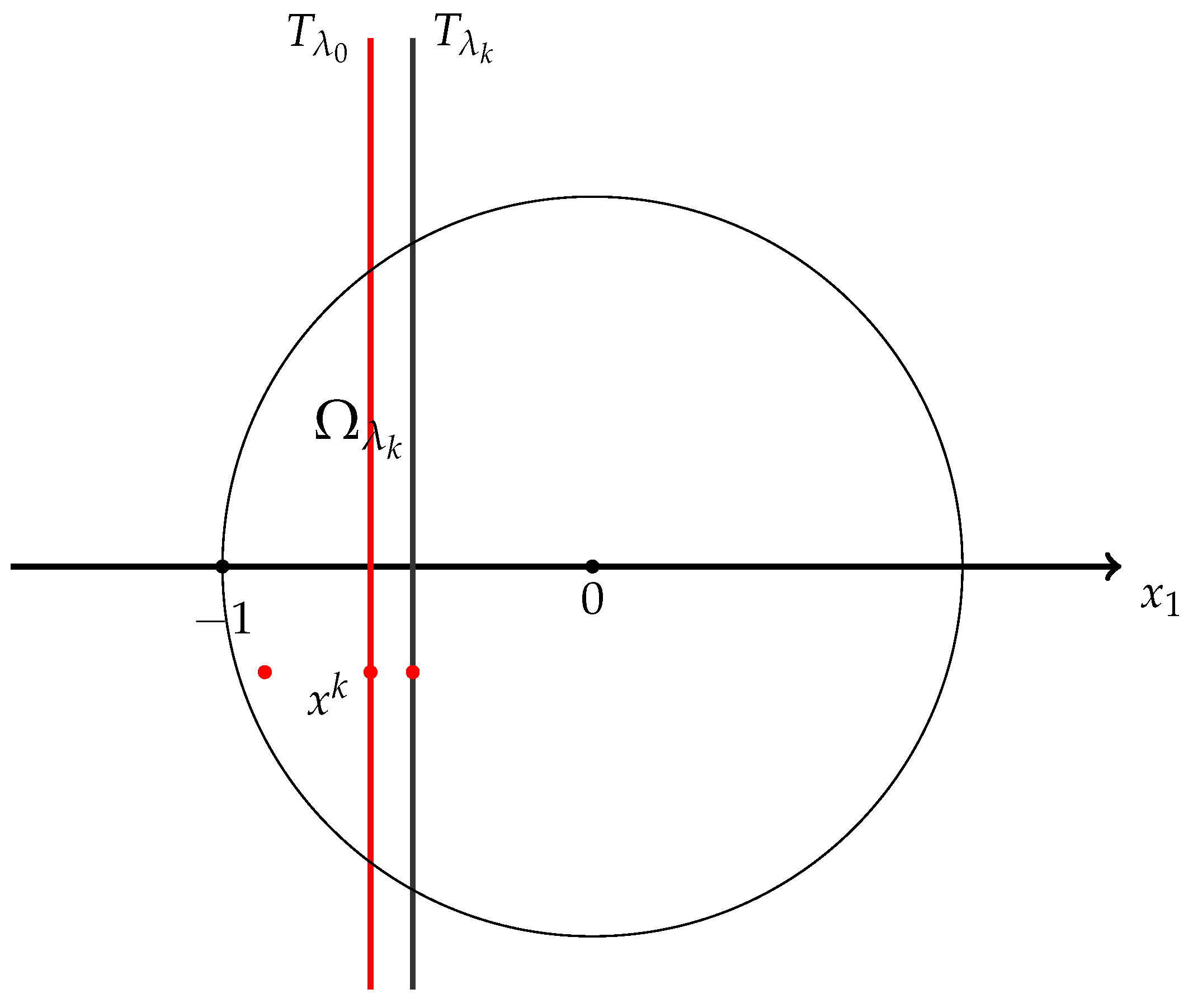
To prove (32), we again argue by contradiction. Suppose ${\lambda }_0<0$, then by the definition of ${\lambda }_0$, there exists a sequence of numbers $\left\{{\lambda }_k\right\}$ with $\left\{{\lambda }_k\right\}\searrow {\lambda }_0$ such that

$$\underset{{\mathsf{\Omega }}_{{\lambda }_k}\times \mathbb{R}}{inf}{w}_{{\lambda }_k}(x,t)=-m_k<0.$$

See Figure 3.

It follows that there exists a sequence $\left\{t_k\right\}\subset \mathbb{R}$ and corresponding $\left\{x\left(t_k\right)\right\}\subset {\mathsf{\Omega }}_{{\lambda }_k}$ such that

$$\begin{array}{c}\hfill w_{{\lambda }_k}(x\left(t_k\right),t_k)=\underset{x\in {\mathsf{\Omega }}_{{\lambda }_k}}{inf}{w}_{{\lambda }_k}(x,t_k)\le -m_k+{\epsilon }_k{m}_k<0.\end{array}$$

Since $\mathbb{R}$ is unbounded, the infimum of $w_{{\lambda }_k}$ with respect to t may not be attained. To estimate ${\displaystyle \frac{\partial w_{{\lambda }_k}}{\partial t}}$, we make a perturbation and let

$$\begin{array}{c}\hfill V_k(x,t):=w_{{\lambda }_k}(x,t)-{\epsilon }_k{m}_k{\eta }_k\left(t\right),\end{array}$$

where ${\eta }_k\left(t\right)=\eta (t-t_k)$ and $\eta \left(t\right)$ is a smooth cut-off function defined by

$$\eta \left(t\right)=\left\{\begin{array}{cc}1,\hfill & t\in (-{\displaystyle \frac{1}{2}},{\displaystyle \frac{1}{2}}),\hfill \\ 0,\hfill & t\notin (-1,1).\hfill \end{array}\right.$$

(33)

It is easy to see that

$$V_k(x\left(t_k\right),t_k)\le -m_k,$$

and

$$V_k(x,t)=w_{{\lambda }_k}(x,t)⩾-m_k$$

for

$$(x,t)\in {\Sigma }_{{\lambda }_k}\times {(t_k-1,t_k+1)}^c.$$

Hence, the auxiliary function $V_k(x,t)$ attains its minimum at some point $(x\left({\overline{t}}_k\right),{\overline{t}}_k)$ in ${\Sigma }_{{\lambda }_k}\times (t_k-1,t_k+1)$ verifying

$$\begin{array}{c}\hfill -m_k-{\epsilon }_k{m}_k\le V_k(x\left({\overline{t}}_k\right),{\overline{t}}_k)=\underset{{\Sigma }_{{\lambda }_k}\times \mathbb{R}}{inf}{V}_k(x,t)\le -m_k.\end{array}$$

(34)

Due to the fact that $w_{{\lambda }_k}(x,t)\ge 0$ in $({\Sigma }_{{\lambda }_k}\setminus {\mathsf{\Omega }}_{{\lambda }_k})\times \mathbb{R}$, the point $(x\left({\overline{t}}_k\right),{\overline{t}}_k)$ is the minimum of $V_k(x,t)$ in ${\mathsf{\Omega }}_{{\lambda }_k}\times \mathbb{R}$, and we simply denote it by $(x^k,t_k)$. Then it follows that

$$\begin{array}{c}\hfill {\displaystyle \frac{\partial V_k}{\partial t}}(x^k,t_k)=0.\end{array}$$

Therefore

$$\begin{array}{c}\hfill {\displaystyle \frac{\partial w_{{\lambda }_k}}{\partial t}}(x^k,t_k)\le C{\epsilon }_k{m}_k.\end{array}$$

(35)

Combining Equations (26) and (35) and the key estimate (the 2s-order derivative-like property), we deduce

$${\displaystyle \frac{C-C{\epsilon }_k}{d{(x^k,T_{{\lambda }_k})}^{2s}}}⩽c_{{\lambda }_k}(x^k,t_k)+C{\epsilon }_k.$$

Since ${\epsilon }_k\to 0$ as $k\to \infty$, and the distance $d(x^k,T_{{\lambda }_k})$ is finite (this time we are not in a narrow region), then for sufficiently large k, it implies that there exists a positive constant $C_0$ independent of k such that, along a subsequence of $\left\{(x^k,t_k)\right\}$, we have

$$c_{{\lambda }_k}(x^k,t_k)\ge C_0>0.$$

Combining this with the condition $f^{\prime }\left(0\right)=0$, we derive

$$u(x^k,t_k)\ge c_1>0.$$

(36)

In fact, if otherwise, then by the continuity assumption of $f^{\prime }(·)$,

$$c_{{\lambda }_k}(x^k,t_k)=f^{\prime }\left({\xi }_{{\lambda }_k}(x^k,t_k)\right)\to f^{\prime }\left(0\right)\le 0.$$

Here we have taken into account that $w_{{\lambda }_k}(x^k,t_k)<0$, and hence

$$u_{{\lambda }_k}(x^k,t_k)\le {\xi }_{{\lambda }_k}(x^k,t_k)\le u(x^k,t_k).$$

Now to continue, a conventional approach is to make a translation in t direction for both functions $w_{{\lambda }_k}$ and u, that is, let

$$w_k(x,t):=w_{{\lambda }_k}(x,t+t_k),\mathrm{and}{u}_k(x,t)=u(x,t+t_k),$$

and take limit as $k\to \infty$. Then derive a contradiction by using both limiting equations. In order that the equations for $w_k$ and $u_k$ converge, it requires very strong regularity assumptions on both sequences $\left\{w_k\right\}$ and $\left\{u_k\right\}$, which cannot be realized for many operators. In particular, it fails when one of the sequences is unbounded.

What we would like to introduce here is a more convenient one—to apply the averaging effect twice, on both $w_{{\lambda }_k}$ and u respectively—to derive a contradiction as k becomes sufficiently large. This approach avoids taking limits along equations, and hence it requires weaker regularity assumptions and can deal with unbounded sequences.

Now we continue from the estimate

$$u(x^k,t_k)\ge c_1>0,\mathrm{for}\mathrm{all}k,$$

(37)

and the fact that

$$w_{{\lambda }_k}(x^k,t_k)<0,\mathrm{for}\mathrm{all}k.$$

(38)

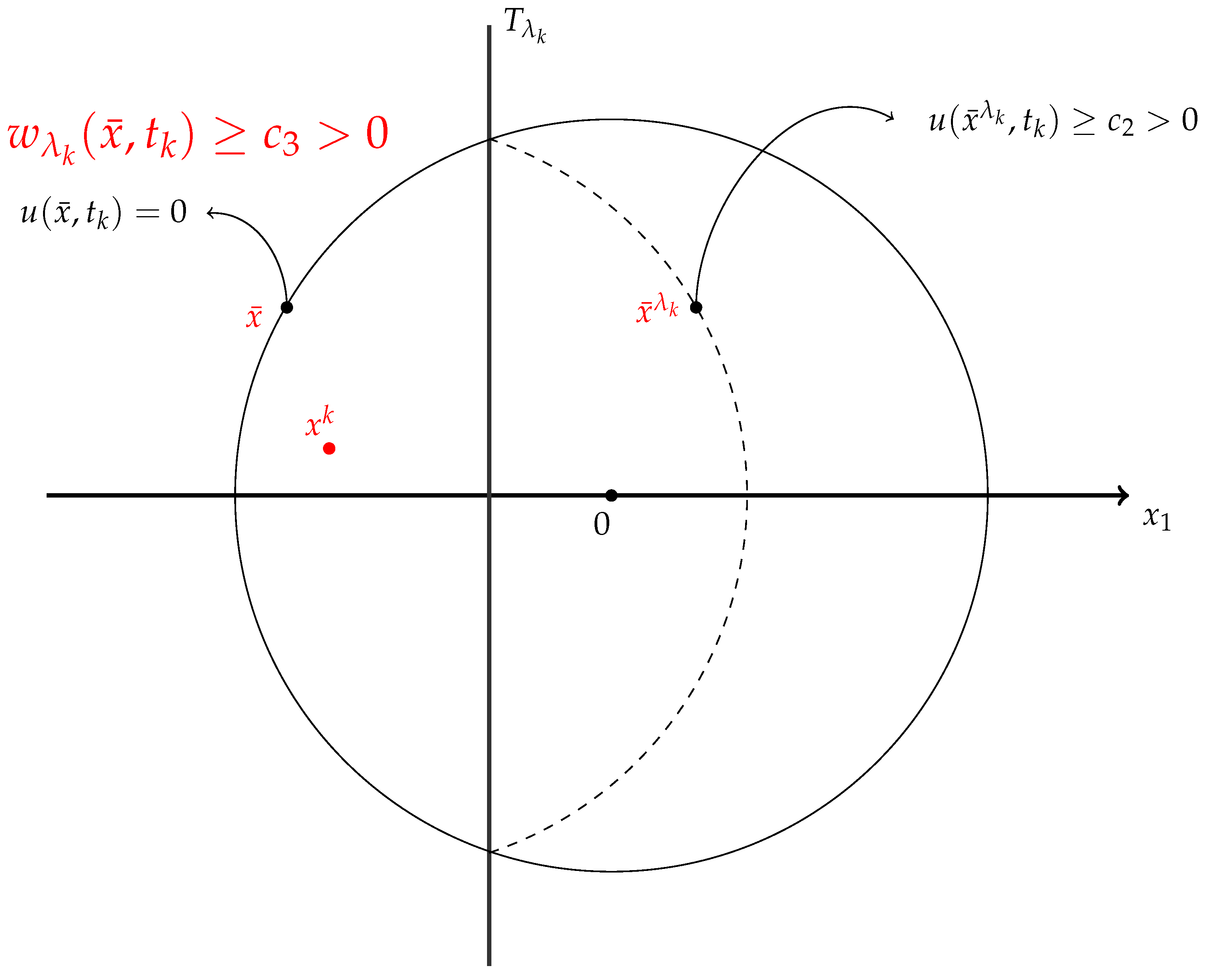
Fix a point $\overline{x}$ on the curve part of the boundary of ${\mathsf{\Omega }}_{{\lambda }_k}$ (see Figure 4 below). Let ${\overline{x}}^{{\lambda }_k}$ be its reflection point about the plane $T_{{\lambda }_k}$. From (37), employing the averaging effect on u, we obtain

$$u({\overline{x}}^{{\lambda }_k},t_k)\ge c_2>0\mathrm{for}\mathrm{all}k.$$

It follows from the definition of $w_{{\lambda }_k}$ that

$$w_{{\lambda }_k}(\overline{x},t_k)\ge c_3>0\mathrm{for}\mathrm{all}k,$$

(39)

because $u(\overline{x},t_k)=0$ on the boundary of $B_1\left(0\right)$.

We are not able to apply the averaging effect directly on $w_{{\lambda }_k}$, because they are not nonnegative. Fortunately, we can utilize $w_{{\lambda }_0}$ who is nonnegative, and by the uniform continuity of u, the difference between the two can be as small as we wish for sufficiently large k. Actually,

$$w_{{\lambda }_k}(\overline{x},t_k)-w_{{\lambda }_0}(\overline{x},t_k)=u({\overline{x}}^{{\lambda }_0},t_k)-u({\overline{x}}^{{\lambda }_k},t_k),$$

while

$$|{\overline{x}}^{{\lambda }_0}-{\overline{x}}^{{\lambda }_k}|=2|{\lambda }_0-{\lambda }_k|\to 0,\mathrm{as}k\to \infty .$$

It follows from this and (39) that

$$w_{{\lambda }_0}(\overline{x},t_k)\ge c_4>0\mathrm{for}\mathrm{all}k.$$

(40)

Now we apply the averaging effect on $w_{{\lambda }_0}$ to derive

$$w_{{\lambda }_0}(x^k,t_k)\ge c_5>0\mathrm{for}\mathrm{all}k.$$

Consequently, by the uniform continuity, we arrive at

$$w_{{\lambda }_k}(x^k,t_k)\ge 0,\mathrm{for}\mathrm{sufficiently}\mathrm{large}k.$$

This contradicts (38) and hence completes the proof. □

3.2. Monotonicity in a Half Space

As another application of the averaging effect, in this section, we consider the fractional equation on a half space

$$\left\{\begin{array}{cc}{(-\Delta )}^{s}u(x,t)=f\left(u\left(x\right)\right),\hfill & x\in {\mathbb{R}}_{+}^n,\hfill \\ u\left(x\right)\equiv 0,\hfill & x\in {\left({\mathbb{R}}_{+}^n\right)}^c.\hfill \end{array}\right.$$

(41)

Here

$${\mathbb{R}}_{+}^n=\{x=(x_1,x^{\prime })\mid x_1>0\}.$$

We will use the method of moving planes to prove that all positive solutions are strictly increasing in $x_1$-direction. This result was established in [34]; here we provide a slightly different and simpler proof.

Previously, when applying the method of moving planes in unbounded domains, one usually requires the solutions to decay to zero in a certain rate or at least be bounded. In [34,48], after introducing a new idea—employing average effect twice on a sequence of solutions—the authors were able to obtain monotonicity for unbounded solutions.

The following are three main ingredients in the process of moving planes. They may also be useful tools in investigating other related problems.

The first one is the narrow region principle for antisymmetric functions in unbounded domains.

Lemma 2 

([34] Narrow region principle for antisymmetric functions). Let Ω be an unbounded narrow region containing the narrow slab

$$\{x\in {\Sigma }_{\lambda }\mid \lambda -2l<x_1<\lambda \}.$$

Suppose that $w\left(x\right)\in (C_{\mathrm{loc}}^{1,1}\left(\mathsf{\Omega }\right)\cap {\mathcal{L}}_{2s}\left({\mathbb{R}}^n\right))$ is lower semi-continuous with respect to x on $\overline{\mathsf{\Omega }}$, and satisfying

$$w\left(x\right)\ge -C(1+|x{|}^{\gamma })forsome0<\gamma <2s,$$

(42)

and

$$\left\{\begin{array}{cc}{(-\Delta )}^{s}w\left(x\right)=c\left(x\right)w\left(x\right),\hfill & x\in \mathsf{\Omega },\hfill \\ w\left(x\right)\ge 0,\hfill & x\in ({\Sigma }_{\lambda }\setminus \mathsf{\Omega }),\hfill \\ w\left(x\right)=-w\left(x^{\lambda }\right),\hfill & x\in {\Sigma }_{\lambda },\hfill \end{array}\right.$$

(43)

where $c(x,t)$ is bounded from above.

Then

$$w\left(x\right)\ge 0,in{\Sigma }_{\lambda }$$

(44)

for sufficiently small l. Furthermore, if $w\left(x\right)$ vanishes at some point $x^0\in \mathsf{\Omega }$, then

$$w\left(x\right)\equiv 0,in{\mathbb{R}}^n.$$

(45)

This narrow region principle is a crucial ingredient in carrying out the method of moving planes as it provides a starting point, from which we will move the plane $T_{\lambda }$ along $x_1$ direction to the right as long as Inequality (44) (with $w\left(x\right)$ replaced by $w_{\lambda }\left(x\right)$) holds. Let

$${\lambda }_0=sup\{\lambda \mid w_{\mu }\left(x\right)\ge 0,\forall x\in {\Sigma }_{\lambda },\mu \le \lambda \}.$$

We will show that ${\lambda }_0=+\infty .$ This is usually done by a contradiction argument. Suppose otherwise, then there exists ${\lambda }_k\searrow {\lambda }_0$ such that $inf{w}_{{\lambda }_k}<0$. To derive a contradiction, a standard approach is to take the limit along a sequence of equations, such as $-\Delta w_k=c_k\left(x\right)w_k\left(x\right)$, to arrive at a limiting equation $-\Delta w\left(x\right)=c\left(x\right)w\left(x\right)$, then to derive a contradiction at the limit equation. This method has been adapted by many authors in a series of the literature. To ensure the convergence of the sequence of equations, higher regularity requirements must be met, and at least, the sequence of solutions must be uniformly bounded.

In order to remove the boundedness assumption on solutions, in [34,48], the authors introduced a brand new idea. Instead of taking the limit along a subsequence of $\left\{w_{{\lambda }_k}\right\}$, they apply the averaging effects twice, first on the solution u, and then on $w_{{\lambda }_0}$, to derive a contradiction for sufficiently large k. We believe that this new approach will become a very useful tool in investigating an unbounded sequence of solutions.

Based on the above narrow region principle and the application of the averaging effect, the author in [34] applied the direct method of moving planes to derive the following monotonicity result.

Theorem 8 

(Monotonicity in a half space I). Let $u\left(x\right)\in C_{\mathrm{loc}}^{1,1}\left({\mathbb{R}}_{+}^n\right)\cap {\mathcal{L}}_{2s}\left({\mathbb{R}}^n\right)$ be a positive solution of (41). Assume that $u\left(x\right)$ is uniformly continuous and satisfies

$$u\left(x\right)\le C(1+|x{|}^{\gamma })forsome0<\gamma <2s.$$

If the nonlinear term $f\in C^1\left([0,+\infty )\right)$ satisfies $f\left(0\right)\ge 0$, $f^{\prime }\left(0\right)\le 0$ and $f^{\prime }$ is bounded from above, then the solution $u\left(x\right)$ is strictly increasing with respect to $x_1$ in ${\mathbb{R}}_{+}^n$.

Sketch of the Proof. 

Let

$$w_{\lambda }\left(x\right)=u\left(x^{\lambda }\right)-u\left(x\right).$$

Then

$${(-\Delta )}^s{w}_{\lambda }\left(x\right)=c_{\lambda }\left(x\right)w_{\lambda }\left(x\right),x\in {\Sigma }_{\lambda }.$$

(46)

In the first step, as usual, we show that for sufficiently small $\lambda$,

$$w_{\lambda }\left(x\right)\ge 0,\forall x\in {\Sigma }_{\lambda }.$$

(47)

This is guaranteed by the narrow region principle stated in Lemma 2.

Inequality (47) provides a starting point to move the plane. Then in the second step, we continously move the plane $T_{\lambda }$ to the right along the $x_1$-axis as long as (47) is valid to its limiting position. Let

$${\lambda }_0:=sup\left\{\lambda \mid w_{\mu }\left(x\right)\ge 0,x\in {\Sigma }_{\mu }\mathrm{for}\mathrm{any}\mu \le \lambda \right\},$$

we will show that

$${\lambda }_0=+\infty .$$

(48)

Otherwise, if ${\lambda }_0<+\infty$, then by its definition, there exists a sequence of ${\lambda }_k>{\lambda }_0$ such that ${\lambda }_k\to {\lambda }_0$ as $k\to \infty$, along which

$${\Sigma }_{{\lambda }_k}^{-}:=\{x\in {\Sigma }_{{\lambda }_k}\mid w_{{\lambda }_k}\left(x\right)<0\}$$

is nonempty and

$${\displaystyle \underset{{\Sigma }_{{\lambda }_k}}{inf}{w}_{{\lambda }_k}\left(x\right)<0.}$$

By the uniform continuity assumption on $u(x,t)$, it is straightforward to show that

$$\underset{{\Sigma }_{{\lambda }_k}}{inf}{w}_{{\lambda }_k}\left(x\right)\to 0ask\to \infty .$$

(49)

With the intention of illustrating the main ideas clearly, we consider the simplest case where the infimum is attained, that is, for each k, there exists a minimum $x^k$:

$${\displaystyle \underset{{\Sigma }_{{\lambda }_k}}{inf}{w}_{{\lambda }_k}\left(x\right)=w_{{\lambda }_k}\left(x^k\right).}$$

In the case when the infimum cannot be attained, we would take a sequence of approximate minima and make perturbations, so that the perturbed functions attain their minima. More details are needed (see [34] or [48]).

Applying the $2s$-order derivative-like property

$${(-\Delta )}^s{w}_{{\lambda }_k}\left(x^k\right)\le {\displaystyle \frac{C{w}_{{\lambda }_k}\left(x^k\right)}{{\left[d(x^k,T_{{\lambda }_k})\right]}^{2s}}},$$

and taking into account that $w_{{\lambda }_k}\left(x^k\right)$ is negative, we arrive at

$${\displaystyle \frac{C}{{\left[d(x^k,T_{{\lambda }_k})\right]}^{2s}}}\le c_{{\lambda }_k}\left(x^k\right).$$

(50)

Here ${\left[d(x^k,T_{{\lambda }_k})\right]}^{2s}$ is the distance between the point $x^k$ and the plane $T_{{\lambda }_k}$.

Inequality (50) implies two consequences.

First, $u\left(x^k\right)$ must be positively bounded away from zero because ${\left[d(x^k,T_{{\lambda }_k})\right]}^{2s}$ is finite. That is, there is $c_o>0$, such that

$$u\left(x^k\right)\ge c_o.$$

(51)

This can be derived from the assumption that $f^{\prime }\left(0\right)\le 0$ and the definition of $c_{\lambda }\left(x\right)$.

Second, since $c_{\lambda }\left(x\right)$ is bounded due to the global Lipschitz assumption on $f(·)$, $d(x^k,T_{{\lambda }_k})$ must also be bounded away from zero:

$$d(x^k,T_{{\lambda }_k})\ge c_1>0.$$

(52)

Now, we are ready to derive a contradiction by applying the averaging effect twice to derive that

$$w_{{\lambda }_k}\left(x^k\right)\ge {\epsilon }_o>0,\mathrm{for}k\mathrm{sufficiently}\mathrm{large},$$

(53)

which contradicts our choice of sequence $\left\{x^k\right\}$, that is, we have chosen $w_{{\lambda }_k}\left(x^k\right)<0$.

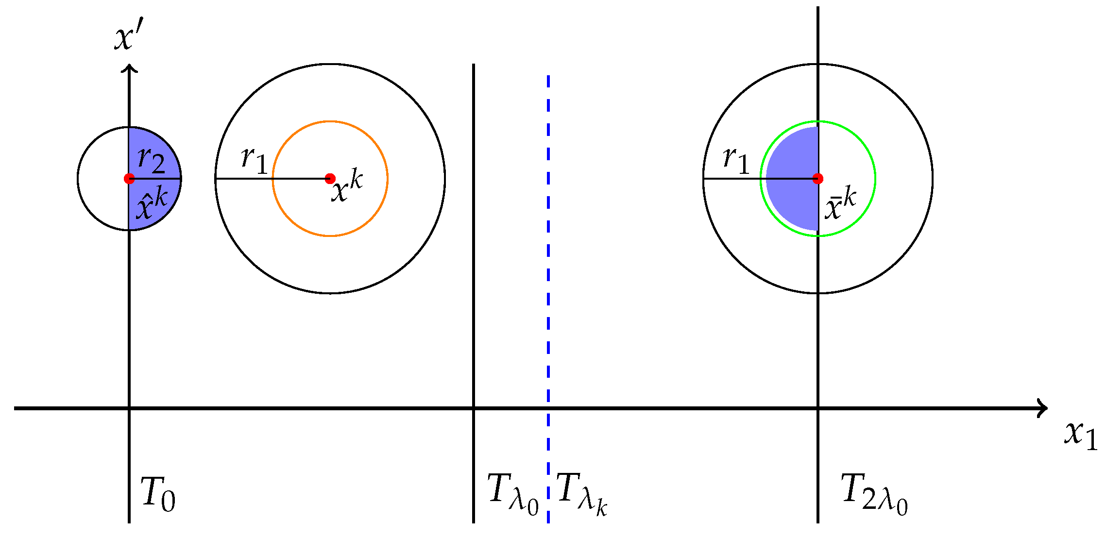
We start from a neighborhood of $x^k$ (see Figure 5 below).

Inequality (51) ensures that the solution $u\left(x\right)$ has a positive lower bound in $B_{r_1}\left(x^k\right)\subset {\Sigma }_{{\lambda }_k}.$ And due to (52), this positive radius $r_1$ can be chosen independent of k.

Then applying the averaging effect on $u\left(x\right)$, we deduce that $u\left(x\right)$ is positively bounded away from zero in a ball of the same size centered at other point ${\overline{x}}^k$ on $T_{2{\lambda }_0}$,

$$u\left(x\right)\ge c_2>0,x\in B_{r_1}\left({\overline{x}}^k\right).$$

(54)

We next apply zero exterior condition in (41) to derive, for sufficiently small $r_2$ (independent of k), and in the ball centered at the point ${\widehat{x}}^k$ on the boundary, that

$$u\left(x\right)\le {\displaystyle \frac{c_2}{2}},x\in B_{r_2}\left({\widehat{x}}^k\right).$$

(55)

Based on (54) and (55), by definition of the antisymmetric function $w_{{\lambda }_0}(x,t)$, we deduce

$$w_{{\lambda }_0}\left(x\right)\ge {\displaystyle \frac{c_2}{2}},x\in B_{r_2}\left({\widehat{x}}^k\right).$$

We further use the averaging effects for antisymmetric functions demonstrated in Lemma 6 to derive that

$$w_{{\lambda }_0}\left(x\right)\ge {\epsilon }_2>0,x\in B_{{\displaystyle \frac{r_1}{2}}}\left(x^k\right).$$

Finally, a combination of the uniform continuity of $w_{\lambda }(x,t)$ with respect to $\lambda$ and ${\lambda }_k\to {\lambda }_0$ as $k\to \infty$ yields that

$$w_{{\lambda }_k}\left(x^k\right)\ge {\displaystyle \frac{{\epsilon }_2}{2}}>0,\mathrm{for}\mathrm{sufficiently}\mathrm{large}k.$$

This contradicts the fact that

$$w_{{\lambda }_k}\left(x^k\right)<0,$$

and hence completes the proof. □

Remark 3. 

The traditional approach is to first make a translation $u_k\left(x\right)=u(x+x^k)$, and take limits along both equations

$${(-\Delta )}^s{w}_k\left(x\right)=c_k\left(x\right)w_k\left(x\right)$$

and

$${(-\Delta )}^s{u}_k\left(x\right)=f\left(u_k\left(x\right)\right),$$

with $w_k\left(x\right)=u_k\left(x^{{\lambda }_k}\right)-u_k\left(x\right)$, to arrive at limiting equations

$${(-\Delta )}^s{w}_0\left(x\right)=c_0\left(x\right)w_0\left(x\right)$$

and

$${(-\Delta )}^s{u}_0\left(x\right)=f\left(u_0\left(x\right)\right).$$

Then try to derive a contradiction at these limiting equations (see, for example, [45]).

In order for the sequences of equations to converge, uniform $C^{2s+ϵ}$ estimates along the solutions must be obtained.

From our above arguments in applying the averaging effects, one can see that only the uniform continuity of the solutions is required.

3.3. Monotonicity in a Half Space Under Weaker Conditions

Employing the more accurate averaging effect—Theorem 3, we will be able to remove the conditions that $f^{\prime }\left(0\right)\le 0$ and $f^{\prime }$ is bounded from above from Theorem 8 and obtain the same monotonicity result.

Theorem 9 

([47]) (Monotonicity in a half space II). Assume $n\ge 2s,$ $f\in C_{loc}^{0,1}\left([0,\infty )\right)$ with $f\left(0\right)\ge 0$ and let $u\in C_{loc}^{1,1}\left({\mathbb{R}}_{+}^n\right)\cap {\mathcal{L}}_{2s}\cap C^0\left(\overline{{\mathbb{R}}_{+}^n}\right)$ be a uniformly continuous, nonnegative, nontrivial classical solution of (41). Then $u\left(x\right)$ is strictly increasing along the $x_n$-direction. Furthermore

$${\displaystyle \frac{\partial u}{\partial x_n}}\left(x\right)>0,\forall x\in {\mathbb{R}}_{+}^n.$$

To prove this theorem, in the second step of the method of moving planes, if the plane $T_{\lambda }$ has to stop somewhere, we would obtain a sequence $\left\{x^k\right\}$ such that $w_{{\lambda }_k}\left(x^k\right)$ approaches its infimum. Applying the averaging effects twice, we deduce that $u\left(x^k\right)\to 0$ as $k\to \infty$. Then we consider the normalized functions

$$v_k\left(x\right)={\displaystyle \frac{u\left(x\right)}{u\left(x_k\right)}},$$

along with their antisymmetric counterparts. Employing the averaging effects once more, together with boundary regularity estimates, we reach a contradiction. For more details, please see [47].

4. Averaging Effect for Nonlocal Monge–Ampère Operators and the Fractional p-Laplacians

Actually, the averaging effects are valid for many other fractional operators, provided that they satisfy suitable maximum principles. In this section, we establish such effects for both the nonlocal Monge–Ampère operators and the fractional p-Laplacians. This serves as a prelude to illustrate the broader applicability of the averaging effects. The proofs presented in this section are somewhat sketchy. Interested readers may fill in the details and further apply these effects to investigate qualitative properties of solutions to equations involving the above-mentioned operators, as well as other nonlocal operators.

4.1. An Averaging Effect for Nonlocal Monge–Ampère Operators

Consider

$${\mathcal{D}}_s^{\theta }u\left(x\right)=inf\left\{P.V.{\int }_{{\mathbb{R}}^n}{\displaystyle \frac{u\left(y\right)-u\left(x\right)}{|A^{-1}{(y-x)|}^{n+2s}}}dy\mid A>0,detA=1,{\lambda }_{min}\left(A\right)\ge \theta >0\right\},$$

with $0<s<1$ and ${\lambda }_{min}\left(A\right)$ being the minimum eigenvalue of the matrix A (see [2]).

Such $D_s^{\theta }$ is uniformly elliptic, and from the definition, it is obvious that

$${\mathcal{D}}_s^{\theta }u\left(x\right)\le -{(-\Delta )}^{s}u\left(x\right).$$

Since the averaging effect is obtained by constructing a sub-solution and applying a maximum principle, we first establish

Theorem 10 

(The maximum principle). Let Ω be a bounded region in ${\mathbb{R}}^n$. Assume that

$$u,v\in C_{\mathrm{loc}}^{1,1}\left(\mathsf{\Omega }\right)\cap C\left(\overline{\mathsf{\Omega }}\right)\cap {\mathcal{L}}_{2s}$$

and satisfies

$$\left\{\begin{array}{cc}{\mathcal{D}}_s^{\theta }u\left(x\right)-{\mathcal{D}}_s^{\theta }v\left(x\right)\le 0\hfill & x\in \mathsf{\Omega }\hfill \\ u\left(x\right)\ge v\left(x\right)\hfill & x\in {\mathsf{\Omega }}^c.\hfill \end{array}\right.$$

(56)

Then

$$u\left(x\right)\ge v\left(x\right),\forall x\in \mathsf{\Omega }.$$

(57)

More strongly, we have either

$$u\left(x\right)>v\left(x\right),\forall x\in \mathsf{\Omega },$$

or

$$u\left(x\right)\equiv v\left(x\right),\forall x\in {\mathbb{R}}^n.$$

Remark 4. 

Notice that ${\mathcal{D}}_s^{\theta }$ is not a linear operator, and hence in general

$${\mathcal{D}}_s^{\theta }u\left(x\right)-{\mathcal{D}}_s^{\theta }v\left(x\right)\ne {\mathcal{D}}_s^{\theta }(u\left(x\right)-v\left(x\right)).$$

Proof. 

Let $w\left(x\right)=u\left(x\right)-v\left(x\right)$. Suppose (57) is violated, then there exists a point $x^0\in \mathsf{\Omega }$, such that

$$w\left(x^0\right)=\underset{x\in \mathsf{\Omega }}{min}w\left(x\right)<0.$$

We will show that

$${\mathcal{D}}_s^{\theta }u\left(x^0\right)-{\mathcal{D}}_s^{\theta }v\left(x^0\right)>0.$$

(58)

In fact, from the definition of the operator, for any $ϵ>0$, there exists a positively definite matrix A with $det\left(A\right)=1$ and ${\lambda }_{min}\left(A\right)\ge \theta >0$, such that

$$\begin{array}{ccc}& & {\mathcal{D}}_s^{\theta }u\left(x^0\right)-{\mathcal{D}}_s^{\theta }v\left(x^0\right)\hfill \\ & \ge & P.V.{\int }_{{\mathbb{R}}^n}{\displaystyle \frac{u\left(y\right)-u\left(x^0\right)}{|A^{-1}(x^0-y){|}^{n+2s}}}dy-ϵ-P.V.{\int }_{{\mathbb{R}}^n}{\displaystyle \frac{v\left(y\right)-v\left(x^0\right)}{|A^{-1}(x^0-y){|}^{n+2s}}}dy\hfill \\ & =& P.V.{\int }_{{\mathbb{R}}^n}{\displaystyle \frac{w\left(y\right)-w\left(x^0\right)}{|A^{-1}(x^0-y){|}^{n+2s}}}dy-ϵ\hfill \\ & \ge & {\theta }^{n+2s}P.V.{\int }_{{\mathbb{R}}^n}{\displaystyle \frac{w\left(y\right)-w\left(x^0\right)}{|x^0{-y|}^{n+2s}}}dy-ϵ\hfill \\ & \ge & {\theta }^{n+2s}P.V.{\int }_{{\mathsf{\Omega }}^c}{\displaystyle \frac{-w\left(x^0\right)}{|x^0{-y|}^{n+2s}}}dy-ϵ.\hfill \end{array}$$

Now let $ϵ\to 0$ and we arrive at (58), which contradicts (56) and thus validates (57).

To verify the strong version of the maximum principle, we suppose that there is a point $x^0\in \mathsf{\Omega }$, such that

$$w\left(x^0\right)=\underset{x\in \mathsf{\Omega }}{min}w\left(x\right)=0.$$

Similar to the above argument, we deduce, for any $ϵ>0$,

$${\mathcal{D}}_s^{\theta }u\left(x^0\right)-{\mathcal{D}}_s^{\theta }v\left(x^0\right)\ge {\theta }^{n+2s}P.V.{\int }_{{\mathbb{R}}^n}{\displaystyle \frac{w\left(y\right)}{|x^0{-y|}^{n+2s}}}dy-ϵ.$$

Letting $ϵ\to 0$ and taking into account of (56), we have

$$P.V.{\int }_{{\mathbb{R}}^n}{\displaystyle \frac{w\left(y\right)}{|x^0{-y|}^{n+2s}}}dy\le 0.$$

Since it is already shown that $w\left(y\right)\ge 0,x\in {\mathbb{R}}^n$, we must have

$$w\left(y\right)\equiv 0,x\in {\mathbb{R}}^n.$$

This completes the proof of the theorem. □

Based on the above maximum principle, we are ready to prove

Theorem 11. 

Let D be a region in ${\mathbb{R}}^n$ and assume that

$$u\left(x\right)⩾c_0>0,x\in D.$$

(59)

Suppose that

$${\mathcal{D}}_s^{\theta }u\left(x\right)⩽\delta in{B}_1\left(\overline{x}\right)$$

for some sufficiently small $\delta >0$ depending on the distance between D and $B_1\left(\overline{x}\right)$; and

$$u\left(x\right)⩾0in{B}_1^c\left(\overline{x}\right),$$

for any $\overline{x}$ such that $B_1\left(\overline{x}\right)$ is disjointed from D. Then there exists a constant $c_1>0$ depending on $c_0$ and the distance between $\overline{x}$ and D, such that

$$u\left(\overline{x}\right)⩾c_1.$$

From the above theorem, one can easily derive the following

Corollary 3. 

Suppose u is uniformly continuous, nonnegative, and at some point $x^0$,

$$u\left(x^0\right)=c_0>0.$$

Assume that

$${\mathcal{D}}_s^{\theta }u\left(x\right)⩽\delta inaneighborhoodofanotherpoint\overline{x}$$

for some sufficiently small $\delta >0$.

Then there exists a constant $ϵ>0$ depending on $c_0$ and the distance between $x^0$ and $\overline{x}$, such that

$$u\left(\overline{x}\right)⩾ϵ.$$

Proof of Theorem 11. 

Let ${\chi }_D\left(x\right)$ be the characteristic function as defined before. Let $\eta \left(x\right)$ be a smooth cut-off function in the unit ball

$$\eta \left(x\right)=\left\{\begin{array}{cc}1,\hfill & x\in B_{\frac{1}{2}}\left(\overline{x}\right),\hfill \\ 0,\hfill & x\in B_1^c\left(\overline{x}\right).\hfill \end{array}\right.$$

Let

$$\underline{u}\left(x\right)={\chi }_D\left(x\right)u\left(x\right)+ϵ\eta \left(x\right).$$

By the definition of the operator, for any given ${ϵ}_1>0$, there exists a matrix A in the family

$$\mathcal{M}:=\{A\mid A>0,detA=1,{\lambda }_{min}\left(A\right)\ge \theta >0\}$$

such that

$$\begin{array}{ccc}\hfill {\mathcal{D}}_s^{\theta }\underline{u}\left(x\right)& =& \underset{\mathcal{M}}{inf}\left\{P.V.{\int }_{{\mathbb{R}}^n}{\displaystyle \frac{\underline{u}\left(y\right)-\underline{u}\left(x\right)}{|A^{-1}{(y-x)|}^{n+2s}}}dy\right\}\hfill \\ & \ge & {\int }_{{\mathbb{R}}^n}{\displaystyle \frac{\underline{u}\left(y\right)-\underline{u}\left(x\right)}{|A^{-1}{(y-x)|}^{n+2s}}}dy-{ϵ}_1\hfill \\ & =& {\int }_D{\displaystyle \frac{u\left(y\right)}{|A^{-1}{(y-x)|}^{n+2s}}}dy+ϵ{\int }_{{\mathbb{R}}^n}{\displaystyle \frac{\eta \left(x\right)-\eta \left(y\right)}{|A^{-1}{(y-x)|}^{n+2s}}}dy-{ϵ}_1\hfill \\ & \ge & c_2-ϵc_3-{ϵ}_1\ge {\displaystyle \frac{C_2}{2}},\hfill \end{array}$$

□

by choosing $ϵ$ and ${ϵ}_1$ sufficiently small.

Now for $\delta \le {\displaystyle \frac{c_2}{2}}$, we have

$${\mathcal{D}}_s^{\theta }u\left(x\right)-{\mathcal{D}}_s^{\theta }\underline{u}\left(x\right)\le 0,x\in B_1\left(\overline{x}\right).$$

(60)

This verifies the differential inequality for $\underline{u}$ as a sub-solution.

The exterior condition is also satisfied, since

$$u\left(x\right)\ge {\chi }_D\left(x\right)u\left(x\right)=\underline{u}\left(x\right),\forall x\notin B_1\left(\overline{x}\right).$$

(61)

Now by the maximum principle (Theorem 10), we arrive at

$$u\left(x\right)\ge \underline{u}\left(x\right)=ϵ\eta \left(x\right),\forall x\in B_1\left(\overline{x}\right),$$

which implies immediately

$$u\left(\overline{x}\right)\ge ϵ.$$

4.2. An Averaging Effect for the Fractional p-Laplacians

Consider the fractional p-Laplacian defined by

$${(-\Delta )}_p^{s}u\left(x\right)=C_{n,s}PV{\int }_{{\mathbb{R}}^n}{\displaystyle \frac{{|u\left(x\right)-u\left(y\right)|}^{p-2}(u\left(x\right)-u\left(y\right))}{{|x-y|}^{n+ps}}}dy.$$

We first recall the maximum principle.

Theorem 12. 

Let Ω be a bounded region in ${\mathbb{R}}^n$. Assume that $u,v\in {\mathcal{L}}_{sp}\cap C_{loc}^{1,1}\cap C\left(\overline{\mathsf{\Omega }}\right)$. If

$$\left\{\begin{array}{cc}{(-\Delta )}_p^{s}u\left(x\right)-{(-\Delta )}_p^{s}v\left(x\right)\ge 0\hfill & in\mathsf{\Omega },\hfill \\ u\left(x\right)-v\left(x\right)\ge 0\hfill & in{\mathbb{R}}^n\setminus \mathsf{\Omega },\hfill \end{array}\right.$$

(62)

then

$$u\left(x\right)-v\left(x\right)\ge 0in\mathsf{\Omega }.$$

(63)

If $u\left(x\right)-v\left(x\right)=0$ at some point in Ω, then

$$u\left(x\right)-v\left(x\right)=0almosteverywherein{\mathbb{R}}^n.$$

These conclusions hold for unbounded region Ω if we further assume that

$$\underset{\left|x\right|\to \infty }{\underline{lim}}[u\left(x\right)-v\left(x\right)]\ge 0.$$

The proof is similar to that of Theorem 2.2 in [18], so we skip it here.

Now we are ready to state the averaging effects for fractional p-Laplacians.

Theorem 13. 

Let D be a region in ${\mathbb{R}}^n$ and assume that

$$u\left(x\right)⩾c_0>0,x\in D.$$

(64)

Suppose that

$${(-\Delta )}_p^{s}u\left(x\right)⩾-\delta in{B}_1\left(\overline{x}\right)$$

for some sufficiently small $\delta >0$ depending on the distance between D and $B_1\left(\overline{x}\right)$; and

$$u\left(x\right)⩾0in{B}_1^c\left(\overline{x}\right),$$

for any $\overline{x}$ such that $B_1\left(\overline{x}\right)$ is disjointed from D. Then there exists a constant $ϵ>0$ depending on $c_0$ and the distance between $\overline{x}$ and D, such that

$$u\left(\overline{x}\right)⩾ϵ.$$

The following analysis lemma is needed in the proof.

Lemma 3 

([18]). For $G\left(z\right)={\left|z\right|}^{p-2}z,p>2$, there exists a constant $C>0$ such that

$$G\left(z_2\right)-G\left(z_1\right)\ge c{(z_2-z_1)}^{p-1}forarbitrary{z}_2>z_1\ge 0.$$

Proof of Theorem 13. 

Let $\eta \left(x\right)$ be the smooth cut-off function as defined in the proof of Theorem 11. Still set

$$\underline{u}\left(x\right)={\chi }_D\left(x\right)u\left(x\right)+ϵ\eta \left(x\right).$$

By the definition of ${(-\Delta )}_p^s$ and Lemma 3, for any $x\in B_1\left(\overline{x}\right)$, we calculate

$$\begin{array}{cc}\hfill & {(-\Delta )}_p^s\underline{u}\left(x\right)={(-\Delta )}_p^s[{\chi }_D\left(x\right)u\left(x\right)+ϵ\eta \left(x\right)]\hfill \\ \hfill & =C_{n,sp}P.V.{\int }_{{\mathbb{R}}^n}{\displaystyle \frac{G(ϵ\eta \left(x\right)-{\chi }_D\left(y\right)u\left(y\right)-ϵ\eta \left(y\right))}{{|x-y|}^{n+sp}}}dy\hfill \\ \hfill & =C_{n,sp}P.V.\{{\int }_{B_1\left(\overline{x}\right)}{\displaystyle \frac{G\left(ϵ\eta \right(x)-ϵ\eta (y\left)\right)}{{|x-y|}^{n+sp}}}dy+{\int }_D{\displaystyle \frac{G\left(ϵ\eta \right(x)-u(y\left)\right)}{{|x-y|}^{n+sp}}}dy\hfill \\ \hfill & +{\int }_{{\mathbb{R}}^n\setminus (B_1\left(\overline{x}\right)\cup D)}{\displaystyle \frac{G\left(ϵ\eta \right(x\left)\right)}{{|x-y|}^{n+sp}}}dy+{\int }_D{\displaystyle \frac{G\left(ϵ\eta \right(x\left)\right)}{{|x-y|}^{n+sp}}}dy-{\int }_D{\displaystyle \frac{G\left(ϵ\eta \right(x\left)\right)}{{|x-y|}^{n+sp}}}dy\}\hfill \\ \hfill & ={(-\Delta )}_p^s\left(ϵ\eta \left(x\right)\right)+{\int }_D{\displaystyle \frac{G\left(ϵ\eta \right(x)-u(y\left)\right)-G\left(ϵ\eta \right(x\left)\right)}{{|x-y|}^{n+sp}}}dy\hfill \\ \hfill & \le {(-\Delta )}_p^s\left(ϵ\eta \right)\left(x\right)-{\int }_D{\displaystyle \frac{C{u}^{p-1}\left(y\right)}{{|x-y|}^{n+sp}}}dy\hfill \\ \hfill & \le C_1{ϵ}^{p-1}-C_2,\hfill \end{array}$$

(65)

where $C_2$ is a positive constant and $C_1$ is the upper bound of ${(-\Delta )}_p^s\eta \left(x\right)$.

Estimate (65) implies that

$${(-\Delta )}_p^{s}u\left(x\right)-{(-\Delta )}_p^s\underline{u}\left(x\right)\ge -\delta -C_1{ϵ}^{p-1}+C_2\ge 0,\forall x\in B_1\left(\overline{x}\right)$$

for sufficiently small $\delta$ and $ϵ$. This validates the differential inequality for $\underline{u}$ to be a sub-solution in $B_1\left(\overline{x}\right)$. The exterior condition is obviously satisfied by the definition of $\underline{u}\left(x\right)$.

Now applying the maximum principle (Theorem 12), we arrive at

$$u\left(\overline{x}\right)\ge ϵ\eta \left(\overline{x}\right)=ϵ.$$

This completes the proof. □

5. Limitations and Possible Projects

5.1. Limitations

From the previous sections, one can see that, for many nonlocal operators, the averaging effect can be established and employed in the second step of the method of moving planes to derive the monotonicity and symmetry of solutions. However, this approach does have certain limitations. For instance, it can only be applied to nonnegative solutions that are uniformly continuous. Moreover, the nonlocal operators under consideration are required to satisfy suitable maximum principles.

5.2. Possible Projects

Thus far, we have only applied this approach in the method of moving planes. Whether it can also be employed in the sliding method has not yet been investigated. Interested readers may wish to explore this direction.

Based on the averaging effects established in Section 4, one may also try to apply them to the study of qualitative properties of nonlocal Monge–Ampère equations and fractional p-Laplace equations. Another interesting direction is to establish this effect for other types of nonlocal operators, such as the fully fractional parabolic operator ${({\partial }_t-\Delta )}^s$, as well as mixed local and nonlocal operators of the form

$$-\Delta +{(-\Delta )}^s,$$

together with the corresponding mixed parabolic operators. One may then investigate the qualitative properties of the associated equations.

References

1. Stein, E. Singular Integrals and Differentiability Properties of Functions; Princeton University Press: Princeton, NJ, USA, 1970. [Google Scholar]
2. Caffarelli, L.; Silvestre, L. A nonlocal Monge-Ampère equation. Commun. Anal. Geom. 2016, 24, 307–335. [Google Scholar] [CrossRef]
3. Caffarelli, L.; Roquejoffre, J.-M.; Savin, O. Nonlocal minimal surfaces. Commun. Pure Appl. Math. 2010, 63, 1111–1144. [Google Scholar] [CrossRef]
4. Caffarelli, L.A.; Salsa, S.; Silvestre, L. Regularity estimates for the solution and the free boundary of the obstacle problem for the fractional Laplacian. Invent. Math. 2008, 171, 425–461. [Google Scholar] [CrossRef]
5. Caffarelli, L.; Valdinoci, E. Uniform estimates and limiting arguments for nonlocal minimal surfaces. Calc. Var. Partial. Differ. Equ. 2011, 41, 203–240. [Google Scholar] [CrossRef]
6. González, M.d.M.; Monneau, R. Slow motion of particle systems as a limit of a reaction diffusion equation with half-Laplacian in dimension one. Discret. Contin. Dyn. Syst. 2012, 32, 1255–1286. [Google Scholar] [CrossRef]
7. Metzler, R.; Klafter, J. The random walk’s guide to anomalous diffusion: A fractional dynamics approach. Phys. Rep. 2000, 339, 1–77. [Google Scholar] [CrossRef]
8. Sire, Y.; Valdinoci, E. Fractional Laplacian phase transitions and boundary reactions: A geometric inequality and a symmetry result. J. Funct. Anal. 2009, 256, 1842–1864. [Google Scholar] [CrossRef]
9. Valdinoci, E. From the long jump random walk to the fractional Laplacian. Bol. Soc. Esp. Mat. Apl. SeMA 2009, 49, 33–44. [Google Scholar]
10. Caffarelli, L.; Silvestre, L. An extension problem related to the fractional Laplacian. Commun. Partial Differ. Equ. 2007, 32, 1245–1260. [Google Scholar] [CrossRef]
11. Brändle, C.; Colorado, E.; de Pablo, A.; Sánchez, U. A concave-convex elliptic problem involving the fractional Laplacian. Proc. R. Soc. Edinb. Sect. Math. 2013, 143, 39–71. [Google Scholar] [CrossRef]
12. Chen, W.; Li, C.; Ou, B. Classification of solutions for an integral equation. Commun. Pure Appl. Math. 2006, 59, 330–343. [Google Scholar] [CrossRef]
13. Hang, F. On the integral systems related to Hardy-Littlewood-Sobolev inequality. Math. Res. Lett. 2007, 14, 373–383. [Google Scholar] [CrossRef]
14. Han, X.; Lu, G.; Zhu, J. Characterization of balls in terms of Bessel-potential integral equation. J. Differ. Equ. 2012, 252, 1589–1602. [Google Scholar] [CrossRef]
15. Ma, L.; Chen, D. A Liouville type theorem for an integral system. Commun. Pure Appl. Math. 2006, 5, 855–859. [Google Scholar]
16. Ma, L.; Zhao, L. Classification of positive solitary solutions of the nonlinear Choquard equation. Arch. Ration. Mech. Anal. 2010, 195, 455–467. [Google Scholar] [CrossRef]
17. Chen, W.; Li, C.; Li, Y. A direct method of moving planes for the fractional Laplacian. Adv. Math. 2017, 308, 404–437. [Google Scholar] [CrossRef]
18. Chen, W.; Li, C. Maximum principles for the fractional p-Laplacian and symmetry of solutions. Adv. Math. 2018, 335, 735–758. [Google Scholar] [CrossRef]
19. Barrios, B.; Peral, I.; Soria, F.; Valdinoci, E. A Widder’s type theorem for the heat equation with nonlocal diffusion. Arch. Ration. Mech. Anal. 2014, 213, 629–650. [Google Scholar] [CrossRef]
20. Bucur, C.; Valdinoci, E. Nonlocal Diffusion and Applications; Springer International Publishing: Cham, Switzerland, 2016. [Google Scholar]
21. Čiegis, R.; Dapšys, I.; Čiegis, R. A Comparison of parallel algorithms for numerical solution of parabolic problems with fractional power elliptic operators. Axioms 2022, 11, 98. [Google Scholar] [CrossRef]
22. Chen, W.; Guo, Y. Dual fractional parabolic equations with indefinite nonlinearities. Adv. Math. 2024, 455, 109891. [Google Scholar] [CrossRef]
23. Chen, W.; Li, Y.; Zhang, R. A direct method of moving spheres on fractional order equations. J. Funct. Anal. 2017, 272, 4133–4157. [Google Scholar]
24. Li, C.; Xu, M.; Yang, H.; Zhuo, R. The direct moving sphere for fractional Laplace equation. J. Funct. Anal. 2025, 289, 29. [Google Scholar] [CrossRef]
25. Chen, W.; Li, C.; Li, Y. A direct blow-up and rescaling argument on nonlocal elliptic equations. Int. J. Math. 2016, 27, 1650064. [Google Scholar] [CrossRef]
26. Berestycki, H.; Caffarelli, L.A.; Nirenberg, L. Monotonicity for elliptic equations in unbounded Lipschitz domains. Commun. Pure Appl. Math. 1997, 50, 1089–1111. [Google Scholar] [CrossRef]
27. Berestycki, H.; Nirenberg, L. On the method of moving planes and the sliding method. Bol. Soc. Bras. Mat. (N. S.) 1991, 22, 1–37. [Google Scholar] [CrossRef]
28. Berestycki, H.; Hamel, F.; Monneau, R. One-dimensional symmetry of bounded entire solutions of some elliptic equations. Duke Math. J. 2000, 103, 375–396. [Google Scholar] [CrossRef]
29. Chen, W.; Hu, Y.; Ma, L. Moving planes and sliding methods for fractional elliptic and parabolic equations. Adv. Nonlinear Stud. 2024, 24, 359–398. [Google Scholar] [CrossRef]
30. Guo, Y.; Ma, L.; Zhang, Z. Sliding methods for dual fractional nonlinear divergence type parabolic equations and the Gibbons’ conjecture. Adv. Nonlinear Stud. 2024, 24, 279–302. [Google Scholar] [CrossRef]
31. Barrios, B.; Garćıa-Melian, J.; Quaas, A. A note on the monotonicity of solutions for fractional equations in half-spaces. Proc. Am. Math. Soc. 2019, 147, 3011–3019. [Google Scholar] [CrossRef]
32. Li, C.; Wu, Z.; Xu, H. Maximum principles and Bôcher type theorems. Proc. Natl. Acad. Sci. USA 2018, 115, 6976–6979. [Google Scholar] [CrossRef]
33. Dai, W.; Liu, Z.; Lu, G. Liouville type theorems for PDE and IE systems involving fractional Laplacian on a half space. Potential Anal. 2017, 46, 569–588. [Google Scholar] [CrossRef]
34. Li, Y. A semilinear Dirichlet problem involving the fractional Laplacian in R + n . Adv. Nonlinear Stud. 2024, 24, 451–462. [Google Scholar] [CrossRef]
35. Lu, G.; Zhu, J. An overdetermined problem in Riesz-potential and fractional Laplacian. Nonlinear Anal. 2012, 75, 3036–3048. [Google Scholar] [CrossRef]
36. Dai, W.; Qin, G. Classification of nonnegative classical solutions to third-order equations. Adv. Math. 2018, 328, 822–857. [Google Scholar] [CrossRef]
37. Fall, M. Entire s-harmonic functions are affine. Proc. AMS 2016, 144, 2587–2592. [Google Scholar] [CrossRef]
38. Frank, R.L.; Lenzmann, E.; Silvestre, L. Uniqueness of radial solutions for the fractional Laplacian. arXiv 2013, arXiv:1302.2652v1. [Google Scholar] [CrossRef]
39. Zhuo, R.; Li, C. Classification of anti-symmetric solutions to nonlinear fractional Laplace equations. Calc. Var. 2022, 61, 17. [Google Scholar] [CrossRef]
40. Ros-Oton, X.; Serra, J. The Dirichlet problem for the fractional Laplacian: Regularity up to the boundary. Math. Pures Appl. 2014, 101, 275–302. [Google Scholar] [CrossRef]
41. Silvestre, L. Regularity of the obstacle problem for a fractional power of the Laplace operator. Commun. Pure Appl. Math. 2007, 60, 67–112. [Google Scholar] [CrossRef]
42. Barrios, B.; Pezzo, L.D.; Garcia-Melian, J.; Quaas, A. A priori bounds and existence of solutions for some nonlocal elliptic problems. Rev. Mat. Iberoam. 2018, 34, 195–220. [Google Scholar] [CrossRef]
43. Jin, T.; Li, Y.Y.; Xiong, J. On a fractional Nirenberg problem, part I: Blow up analysis and compactness of solutions. J. Eur. Math. Soc. 2014, 16, 1111–1171. [Google Scholar] [CrossRef]
44. Caffarelli, L.; Vasseur, A. Drift diffusion equations with fractional diffusion and the quasi-geostrophic equation. Ann. Math. 2010, 171, 1903–1930. [Google Scholar] [CrossRef]
45. Chen, W.; Wu, L. Liouville theorems for fractional parabolic equations. Adv. Nonlinear Stud. 2021, 21, 939–958. [Google Scholar] [CrossRef]
46. Liu, M.; Zhang, L.; Wang, G. Radial symmetry, monotonicity and Liouville theorem for Marchaud fractional parabolic equations with the nonlocal Bellman operator. Adv. Nonlinear Stud. 2025, 25, 902–920. [Google Scholar] [CrossRef]
47. Chen, W.; Guo, Y.; Wu, L. Monotonicity for fractional semi-linear problem in a half space. arXiv 2026, arXiv:2603.14627. [Google Scholar] [CrossRef]
48. Chen, W.; Ma, L. Qualitative properties of solutions for dual fractional nonlinear parabolic equations. J. Funct. Anal. 2023, 285, 110117. [Google Scholar] [CrossRef]
Figure 1. The positiveness of u in D is diffused to B 1 ( x ¯ ) .
Fractalfract 10 00360 g001
Figure 2. The positions of B r ( x 0 ) , B r ( ( x 0 ) λ ) , D, and D λ .
Fractalfract 10 00360 g002
Figure 3. The hyperplane sequence { T λ k } .
Fractalfract 10 00360 g003
Figure 4. Locations of the sequence.
Fractalfract 10 00360 g004
Figure 5. The positions of the balls.
Fractalfract 10 00360 g005
Disclaimer/Publisher’s Note: The statements, opinions and data contained in all publications are solely those of the individual author(s) and contributor(s) and not of MDPI and/or the editor(s). MDPI and/or the editor(s) disclaim responsibility for any injury to people or property resulting from any ideas, methods, instructions or products referred to in the content.