Article

A Compact Finite Difference Scheme with Second-Order Temporal and Sixth-Order Spatial Accuracy for Variable-Order Time-Fractional Sub-Diffusion Equations


Department of Mathematics, Yanbian University, Yanji 133000, China
*
Author to whom correspondence should be addressed.
Fractal Fract. 2026, 10(5), 347; https://doi.org/10.3390/fractalfract10050347
Submission received: 16 April 2026 / Revised: 12 May 2026 / Accepted: 15 May 2026 / Published: 21 May 2026
(This article belongs to the Special Issue Advanced Numerical Methods for Fractional Functional Models)

Abstract

In this paper, a finite difference scheme is proposed for the variable-order time-fractional sub-diffusion equation, achieving second-order accuracy in time and sixth-order accuracy in space. For spatial discretization, a newly constructed operator A is employed to obtain a sixth-order compact approximation of the second derivative. Using an energy analysis method, a priori estimates of the scheme are derived, and the unconditional stability and convergence are rigorously proved. Numerical examples are provided to verify the theoretical accuracy of the scheme.

1. Introduction

Anomalous diffusion phenomena are widely observed in nature and engineering, such as pollutant transport in porous media, drug delivery in biological tissues, and price fluctuations in option pricing. Classical diffusion equations are based on the assumption of Brownian motion, where the mean square displacement scales linearly with time. However, a large number of experimental observations indicate that many practical diffusion processes do not follow this law; instead, they exhibit sub-diffusion or super-diffusion. To characterize such anomalous diffusion processes, fractional-order differential equations have gradually become a powerful mathematical tool, whose nonlocal memory effects and hereditary properties can naturally describe long-range correlations in complex systems.
Constant-order fractional differential equations have achieved great success in modeling anomalous diffusion, but their diffusion exponent γ is usually assumed to be constant, making it difficult to describe situations where the diffusion characteristics vary with space or time. For example, in heterogeneous media, the physical properties of the medium may vary with space; in complex dynamical processes, the memory intensity of the system may change over time. To overcome this limitation, Samko and Ross first proposed the concept of variable-order fractional calculus in 1993 [1]. Subsequently, Lorenzo and Hartley systematically developed the theory of variable-order and distributed-order fractional operators [2]. Coimbra introduced a physically meaningful variable-order derivative definition from a mechanical perspective [3]. Variable-order fractional models can dynamically adjust the order of differentiation, thus more delicately capturing the non-uniform memory and hereditary properties of systems [4]. In recent years, variable-order fractional differential equations have found increasingly wide applications in fields such as groundwater contamination, soft matter physics, viscoelastic mechanics, and signal processing [5]. In particular, for anomalous diffusion modeling, Sun et al. pointed out that variable-order fractional operators can more realistically reflect the variation of the diffusion exponent as the process evolves [6]. Very recently, Sibatov et al. provided a physical interpretation of variable-order fractional sub-diffusion equations within the multiple trapping model and developed Monte Carlo simulation methods [7].
The development of numerical methods for variable-order fractional models has undergone significant evolution over the past two decades. Initial investigations in this field predominantly adopted first-order temporal approximations as the standard approach. Among these pioneering efforts, Chen and colleagues [8] established foundational stability and convergence results using Fourier analysis for their finite difference discretization. As computational requirements grew more demanding, researchers shifted attention toward achieving higher temporal precision. This shift led to the emergence of second-order temporal discretization as a central research theme. Zhao and collaborators [9] made fundamental contributions by deriving two distinct second-order approximation formulas for the variable-order Caputo operator, thereby providing essential theoretical tools for temporal discretization. Subsequent research by Du et al. [10] extended these ideas to multi-dimensional settings with rigorous mathematical proofs using energy inequality techniques. Cao’s research group [11] introduced a Crank–Nicolson type formulation achieving both second-order temporal and fourth-order spatial accuracy. Zhang and associates [12] further broadened this framework by incorporating fourth-order spatial derivative terms. Most recently, Zhang and coworkers [13] developed a computationally efficient algorithm leveraging the L2-1 σ formula combined with exponential sum approximation techniques. Complementary to these developments, adaptive time-stepping strategies [14] and advanced stable algorithms [15] have also been proposed.
Although the above methods achieve second-order accuracy in time, spatial discretization is mostly limited to second or fourth order. When high-resolution simulations are required for long-time behavior or solutions with rapidly varying spatial features, low-order spatial discretizations often lead to excessively fine computational grids, significantly increasing computational cost. Therefore, developing higher-order spatial discretization schemes is of great practical importance.
Significant advances in spatial discretization have been achieved for constant-order fractional models. Zhou and colleagues [16] developed a sixth-order spatial approximation tailored for variable-coefficient sub-diffusion problems, demonstrating temporal convergence of order (2- α ). An alternative approach by Roul et al. [17] integrated the L1 temporal discretization with sextic B-spline basis functions, establishing sixth-order spatial convergence. Zhang and collaborators [18] presented a comprehensive sixth-order numerical framework accompanied by rigorous convergence proofs of order O ( τ 2 + h 6 ) . Dehghan and Safarpoor [19] introduced a non-uniform grid formulation using combined compact operators for multi-term diffusion-wave problems. Additionally, Soori et al. [20] investigated alternating direction implicit techniques with sixth-order spatial precision for two-dimensional wave phenomena. It is important to note that these approaches are inherently designed for constant-order fractional operators and lack direct applicability to the variable-order context.
Within the variable-order paradigm, investigations into sixth-order spatial approximations remain limited. Lu and associates [21] introduced an approach that integrates exponential sum approximation with combined compact difference operators, attaining sixth-order spatial accuracy through a three-point CCD formulation with numerical validation. Nevertheless, their temporal discretization relies on exponential sum approximation, which constrains temporal accuracy and consequently limits performance in long-duration high-precision computations. Spectral collocation techniques utilizing Chebyshev polynomials of the sixth kind and meshless approaches have also demonstrated high-order spatial accuracy for variable-order problems. However, these methods operate within spectral or meshless frameworks and diverge substantially from finite difference approaches in terms of algorithmic simplicity, computational complexity, and mathematical tractability.
Despite these advances, a finite difference discretization achieving simultaneous second-order temporal and sixth-order spatial accuracy for variable-order time-fractional sub-diffusion equations remains unexplored. While the presence of a second-order spatial derivative in principle facilitates sixth-order spatial approximation, two fundamental challenges persist: (i) the interplay between variable-order Caputo temporal discretization and sixth-order spatial operators complicates stability analysis; and (ii) establishing rigorous convergence proofs while preserving computational efficiency presents a non-trivial mathematical obstacle.
Motivated by recent work on sixth-order compact discretizations for classical fractional equations [22], this paper develops a new numerical approach for the variable-order time-fractional sub-diffusion equation. Addressing the respective limitations of existing methods—limited spatial accuracy in [10], insufficient temporal accuracy in [21], and a different problem framework in [22]—this paper provides a unified algorithm that is highly accurate, rigorously theoretically guaranteed, and computationally efficient. Drawing on techniques from [10,22], we consider the following model problem
D t α ( t ) 0 C u ( x , t ) = u x x ( x , t ) + f ( x , t ) , ( x , t ) ( 0 , L ) × ( 0 , T ] , u ( 0 , t ) = u ( L , t ) = 0 , t [ 0 , T ] , u ( x , 0 ) = φ ( x ) , x [ 0 , L ] ,
where f ( x , t ) , φ ( x ) are assumed to be sufficiently smooth. D t α ( t ) 0 C g ( t ) [16] denotes the α ( t ) -order time fractional Caputo derivative of the function g ( t ) , defined as
D t α ( t ) 0 C g ( t ) = g ( t ) g ( 0 ) , α ( t ) = 0 , 1 Γ ( 1 α ( t ) ) 0 t g ( s ) ( t s ) α ( t ) d s , 0 < α ( t ) < 1 , g ( t ) , α ( t ) = 1 .
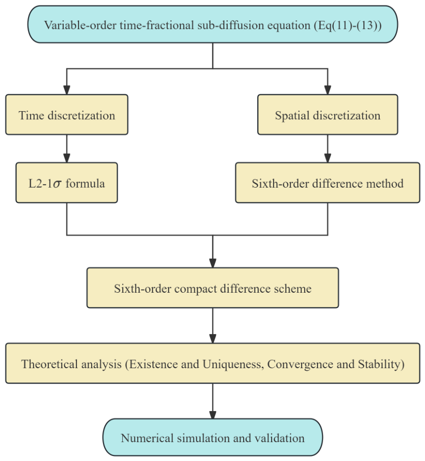
In this paper, we construct a finite difference scheme for the variable-order time-fractional sub-diffusion equation that achieves second-order accuracy in time and sixth-order accuracy in space. We employ a second-order approximation of the variable-order Caputo derivative based on the L2-1 σ formula, ensuring second-order temporal accuracy. For spatial discretization, we use a novel operator configuration to achieve a sixth-order approximation of the second derivative. Through energy analysis method, we derive a priori estimates of the scheme and verify its unconditional stability and convergence. Numerical examples are finally presented to validate the theoretical accuracy of the scheme. This work provides a novel efficient algorithm for high-precision numerical simulation of variable-order fractional diffusion problems and establishes a foundation for further extending the sixth-order spatial scheme to variable-order fractional equations. At last, the structural framework of the paper is shown as Figure 1 below.
The paper is organized as follows. In Section 2, we present the compact difference scheme with second-order temporal accuracy and sixth-order spatial accuracy along with the related notations. Section 3 examines the existence and uniqueness of the fully discrete scheme. A detailed analysis of convergence and stability is presented in Section 4. Section 5 presents numerical calculations that confirm our theoretical findings, and the paper concludes with a brief summary in Section 6.

2. The Compact Finite Difference Scheme

In this section, the L2-1 σ method is mainly used to discretize time, the operator A is used to discretize space, and finally, a compact difference scheme is obtained after processing.
For any integer p, denote set F p = { s | 1 s p , s Z } and F p 0 = { s | 0 s p , s Z } . The intervals [ 0 , L ] and [ 0 , T ] are divided into M and N equal parts, respectively. Take the spatial step length h = L / M and the time step length τ = T / N . Denote x j = j h , j F M 0 , and t n = n τ , n F N 0 . Let Ω h = { x j | j F M 0 } , Ω τ = { t n | n F N 0 } , where M and N are positive integers. Define the grid functions on Ω h as V h = { u | u = ( u 0 , u 1 , , u M ) , u 0 = u M = 0 } .
For any grid functions u V h , introduce the following notations:
δ x u j + 1 2 = 1 h ( u j + 1 u j ) , δ x 2 u j = 1 h 2 ( u j + 1 2 u j + u j 1 ) , ( u , v ) = h j = 1 M 1 u j v j , u = ( u , u ) , | u | 1 = ( δ x u , δ x u ) .
Let
σ n = σ ( t n ) , t n + σ n = t n + σ n τ , α n + σ n = α ( t n + σ n ) .
Here, σ ( t n ) ( 1 2 , 1 ) is the unique root of the equation σ = 1 1 2 α ( t n + σ τ ) , n F N 1 0 ([10]).
For any u = { u i | i F N 0 } defined on Ω τ , σ n in (0,1), we have
u n + σ n = σ n u n + 1 + ( 1 σ n ) u n .
Lemma 1 
([10]). If u C 3 [ 0 , t n + 1 ] , let r n = 0 C D t α ( t ) u ( t ) | t = t n + σ n D α n + σ n u ( t n + σ n ) , we have
| r n | M σ n α n + σ n Γ ( 1 α n + σ n ) [ 1 12 + σ n 6 ( 1 α n + σ n ) ] τ 3 α n + σ n ,
where M = max 0 t t n + 1 | u ( t ) | . Among these,
D α n + σ n u ( t n + σ n ) = τ α n + σ n Γ ( 2 α n + σ n ) k = 0 n c n k ( n , α ) [ u ( t k + 1 ) u ( t k ) ] = β n k = 0 n c k ( n , α ) [ u ( t n k + 1 ) u ( t n k ) ] ,
where β n = τ α n + σ n Γ ( 2 α n + σ n ) , here n = 0 , c 0 ( n , α ) = σ n 1 α n + σ n , when n 1 ,
c l ( n , α ) = 1 2 α n + σ n 1 + σ n 2 α n + σ n σ n 2 α n + σ n 1 2 1 + σ n 1 α n + σ n σ n 1 α n + σ n , l = 0 , 1 2 α n + σ n l + σ n + 1 2 α n + σ n 2 l + σ n 2 α n + σ n + l + σ n 1 2 α n + σ n 1 2 l + σ n + 1 1 α n + σ n 2 l + σ n 1 α n + σ n + l + σ n 1 1 α n + σ n , 1 l n 1 , 1 2 α n + σ n l + σ n 2 α n + σ n l + σ n 1 2 α n + σ n + 1 2 3 l + σ n 1 α n + σ n l + σ n 1 1 α n + σ n , l = n .
Lemma 2 
([22]). Suppose u C ( 10 ) [ x j 1 , x j + 1 ] , we have
A u j = I + 2 h 2 15 δ x 2 u j = 1 15 ( 2 u j 1 + 11 u j + 2 u j + 1 ) ,
B u j = I + h 2 20 δ x 2 u j = 1 20 ( u j 1 + 18 u j + u j + 1 ) ,
then, for the discretization of u x x , we obtain the following approximate formula
A ( u x x ) j = B δ x 2 u j + O ( h 6 ) .
Define the grid functions U on Ω h × Ω τ
U j n = u ( x j , t n ) , j F M 0 , n F N 0 .
Considering the equation of (1) at the point ( x j , t n + σ n ) , we have
D t α ( t n + σ n ) 0 C u ( x j , t n + σ n ) = u x x ( x j , t n + σ n ) + f ( x j , t n + σ n ) , j F M 1 , n F N 1 0 .
Applying the compact operator A to both sides of the above equations, we obtain
A 0 C D t α ( t n + σ n ) u ( x j , t n + σ n ) = A u x x ( x j , t n + σ n ) + A f ( x j , t n + σ n ) , j F M 1 , n F N 1 0 .
By means of Lemma 1 on the left-hand side term of (4), we obtain
A 0 C D t α ( t n + σ n ) u ( x j , t n + σ n ) = β n k = 0 n c k ( n , α ) A ( U j n k + 1 U j n k ) + O ( τ 3 α n + σ n ) .
Using the method in [10] along with Lemma 2, we obtain
A u x x ( x j , t n + σ n ) = A σ n u x x ( x j , t n + 1 ) + ( 1 σ n ) u x x ( x j , t n ) + O ( τ 2 ) = σ n B δ x 2 U j n + 1 + ( 1 σ n ) B δ x 2 U j n + O ( τ 2 + h 6 ) = B δ x 2 ( σ n U j n + 1 + ( 1 σ n ) U j n ) + O ( τ 2 + h 6 ) = B δ x 2 U j n + σ n + O ( τ 2 + h 6 ) .
Substituting (5)–(6) into (4), we have
β n k = 0 n c k ( n , α ) A ( U j n k + 1 U j n k ) = B δ x 2 U j n + σ n + A f j n + σ n + R j n + σ n , j F M 1 , n F N 1 0 ,
where there exists a constant c such that
| R j n + σ n | c ( τ 2 + h 6 ) , j F M 1 , n F N 1 0 .
Omitting the small terms R j n + σ n , substituting U j n with u j n , and noticing boundary conditions
U 0 n = 0 , U M n = 0 , n F N 0 ,
U j 0 = φ ( x j ) , j F M 1 ,
we get the following compact finite difference scheme
β n k = 0 n c k ( n , α ) A ( u j n k + 1 u j n k ) = B δ x 2 u j n + σ n + A f j n + σ n ,
j F M 1 , n F N 1 0 ,
u 0 n = 0 , u M n = 0 , n F N 0 ,
u j 0 = φ ( x j ) , j F M 1 .
In order to conveniently verify the unique solvability, stability, and convergence of the scheme, we manipulate the difference scheme by applying operator A 1 to both sides of the equation, let C = A 1 B , we obtain this compact finite difference scheme:
β n k = 0 n c k ( n , α ) ( u j n k + 1 u j n k ) = C δ x 2 u j n + σ n + f j n + σ n ,
j F M 1 , n F N 1 0 ,
u 0 n = 0 , u M n = 0 , n F N 0 ,
u j 0 = φ ( x j ) , j F M 1 .

3. Existence and Uniqueness

The existence and uniqueness of the solution for the compact difference scheme (14)–(16) are proved in this section.
Lemma 3 
([23]). For any α ( t ) ( 0 < α ( t ) < 1 ) and { c l n , α ( 0 l n , n 1 ) } , it holds that
c 0 n , α > c 1 n , α > > c n 1 n , α > c n n , α > 0 ,
c n n , α > 1 α n + σ n 2 n + σ n α n + σ n > 0 .
Lemma 4 
([23]). Let V h be an inner product space, and · , · * is the inner product with the induced norm · * . For any grid function v n V h , n F N 0 , suppose that { c n ( n , α ) } satisfies (17), we have
k = 0 n c k ( n , α ) v n k + 1 v n k , σ n v n + 1 + 1 σ n v n * 1 2 k = 0 n c k n , α ( v n k + 1 * 2 v n k * 2 ) .
For any u , v V h , we define
u , v C = ( C u , δ x 2 v ) ,
then, u , v C are the inner product on V h . We denote
| u | 1 , C 2 = u , u C .
Lemma 5 
([22]). The coefficient matrix of the the scheme (11)(13) is a pentadiagonal and symmetric positive definite matrix as follows:
A = d 1 a b a d 0 a b b a d 0 a b b a d 0 a b a d 1 ,
d 0 = 11 15 β n c 0 + 17 σ n 10 h 2 , d 1 = 11 15 β n c 0 + 35 σ n 20 h 2 , a = 2 15 β n c 0 4 σ n 5 h 2 , b = σ n 20 h 2 .
The coefficient matrix of the the scheme (14)(16) is also symmetric and positive definite matrices.
Theorem 1. 
The compact difference scheme (14)(16) is uniquely solvable.
Proof. 
We prove the statement by induction. First, (15)–(16) uniquely specify u 0 . Now assuming that { u i | i F n 0 } have been given. Then we consider the homogeneous systems corresponding to u n + 1 below:
β n c 0 ( n , α ) u j n + 1 C δ x 2 u j n + 1 = 0 , j F M 1 .
Based on Lemma 5, taking an inner product with u n + 1 on both sides of (19), we obtain
β n c 0 ( n , α ) ( u n + 1 , u n + 1 ) ( C δ x 2 u n + 1 , u n + 1 ) = 0 .
According to ( C δ x 2 u n + 1 , u n + 1 ) = ( δ x 2 u n + 1 , C u n + 1 ) , combining (19) with (20), we have
β n c 0 ( n , α ) u n + 1 2 + | u n + 1 | 1 , C 2 = 0 .
It yields u n + 1 2 = | u n + 1 | 1 , C 2 = 0 , which follows u n + 1 = 0 .
This completes the proof.  □

4. Convergence and Stability Analysis

This section is devoted first to the convergence analysis of the difference scheme (14)–(16), the stability is then established using the Lax Equivalency Theorem.
Lemma 6 
([22]). Denote
c 0 = max 0 t T t α ( t ) Γ ( 1 α ( t ) ) ,
we have
1 c n ( n , α ) β n 2 c 0 .
Lemma 7 
([22]). For any u V h , we obtain
4 5 u 2 A 1 B u , u = C u , u 15 7 u 2 .
Theorem 2. 
Suppose that { u j n | j F M 0 , n F N 0 } is the solution of the following difference scheme
β n k = 0 n c k ( n , α ) ( u j n k + 1 u j n k ) = C δ x 2 u j n + σ n + F j n + σ n ,
j F M 1 , n F N 1 0 ,
u 0 n = 0 , u M n = 0 , n F N 0 ,
u j 0 = φ ( x ) , j F M 1 ,
then, we obtain
| u n | 1 2 | u 0 | 1 2 + 5 c 0 4 max 0 s n 1 F s + σ s 2 , n F N 0 .
Proof. 
Taking an inner product of (21) with δ x 2 u n + σ n , we obtain
( β n k = 0 n c k ( n , α ) ( u n k + 1 u n k ) , δ x 2 u n + σ n ) = ( C δ x 2 u n + σ n , δ x 2 u n + σ n ) + ( F n + σ n , δ x 2 u n + σ n ) .
Using Lemma 4 for the item on the left-hand side of (25), we have
( β n k = 0 n c k ( n , α ) ( u n k + 1 u n k ) , δ x 2 u n + σ n ) β n 2 k = 0 n c k n , α ( | u n k + 1 | 1 2 | u n k | 1 2 ) .
By Lemma 7, the first item on the right-hand side of (25) arrives at
( C δ x 2 u n + σ n , δ x 2 u n + σ n ) = ( C δ x 2 u n + σ n , δ x 2 u n + σ n ) 4 5 δ x 2 u n + σ n 2 .
Applying the Cauchy–Schwarz inequality to the remaining terms in (25), we obtain
( F n + σ n , δ x 2 u n + σ n ) F n + σ n δ x 2 u n + σ n 4 5 δ x 2 u n + σ n 2 + 5 16 F n + σ n 2 .
Substituting (26)–(28) into (25), using Lemma 7, we obtain
β n 2 k = 0 n c k n , α ( | u n k + 1 | 1 2 | u n k | 1 2 ) 5 16 F n + σ n 2 ,
then, we have
k = 0 n c k n , α ( | u n k + 1 | 1 2 | u n k | 1 2 ) 5 8 β n F n + σ n 2 .
Transforming the above equations and applying Lemma 6, we have
c 0 ( n , α ) | u n + 1 | 1 2 k = 0 n 1 ( c k ( n , α ) c k + 1 ( n , α ) ) | u n k | 1 2 + c n ( n , α ) | u 0 | 1 2 + 5 8 β n F n + σ n 2 k = 0 n 1 ( c k ( n , α ) c k + 1 ( n , α ) ) | u n k | 1 2 + c n ( n , α ) | u 0 | 1 2 + 5 c 0 4 F n + σ n 2 .
We know that (24) is true when n = 0 , then we use mathematical induction to prove (24). Assuming (24) is valid for n F l 0 , combined with Lemma 3, we prove that (24) is valid for n = l + 1 .
c 0 ( l , α ) | u l + 1 | 1 2 k = 0 l 1 ( c k ( l , α ) c k + 1 ( l , α ) ) | u l k | 1 2 + c l ( l , α ) | u 0 | 1 2 + 5 c 0 4 F l + σ l 2 k = 0 l 1 ( c k ( l , α ) c k + 1 ( l , α ) ) | u 0 | 1 2 + 5 c 0 4 max 0 s l k 1 F s + σ s 2 + c l ( l , α ) | u 0 | 1 2 + 5 c 0 4 F l + σ l 2 k = 0 l 1 ( c k ( l , α ) c k + 1 ( l , α ) ) + c l ( l , α ) | u 0 | 1 2 + 5 c 0 4 max 0 s l F s + σ s 2 c 0 ( l , α ) | u 0 | 1 2 + 5 c 0 4 max 0 s l F s + σ s 2 .
From the above inequality, we have
| u l + 1 | 1 2 | u 0 | 1 2 + 5 c 0 4 max 0 s l F s + σ s 2 .
This completes the proof.  □
Theorem 3. 
Suppose that u ( x , t ) is the solution of (1) and { u j n | j F M 0 , n F N 0 } is the solution of the difference scheme (11)(13). Denote
e j n = U j n u j n , j F M 0 , n F N 0 ,
then, there exists a constant c such that
e n c ( τ 2 + h 6 ) , n F N 0 .
Proof. 
Subtracting (11)–(13) from (7)–(10), multiplying both sides of the resulting equation by operator A 1 , we obtain the error system
β n k = 0 n c k ( n , α ) ( e j n k + 1 e j n k ) = C δ x 2 e j n + σ n + R j n + σ n , i F M 1 , n F N 1 0 , e 0 n = 0 , e M n = 0 , n F N 0 , e j 0 = 0 , j F M 1 .
Applying Theorem 2 for the above equation, we have
| e n | 1 2 | e 0 | 1 2 + 5 c 0 4 max 0 s n 1 R s + σ s 2 , n F N 0 .
Noticing (8) and (12), we know
| e n | 1 5 c 0 L 4 ( τ 2 + h 6 ) , n F N 0 .
According to the inverse estimate u L 2 | u | 1 , we obtain
e n c ( τ 2 + h 6 ) , n F N 0 ,
where
c = 5 c 0 L 4 .
It completes the proof.  □
For a consistent finite difference scheme, stability is equivalent to convergence (Lax Equivalence Theorem) [24]. Hence, the convergence of our scheme is already ensured by its stability established earlier. To further validate the theoretical results, we now present two numerical examples.

5. Numerical Results

To confirm the theoretical analysis, three numerical examples are provided in this section using the compact scheme (11)–(13) for problem (1). The computations are carried out in Python (3.11.5).
Denote
E ( h , τ ) = max k F N 0 U k u k , o r d e r τ = log 2 E ( h , 2 τ ) E ( h , τ ) , o r d e r h = log 2 E ( 2 h , 8 τ ) E ( h , τ ) .
Example 1. 
Considering Problem (1) with the initial condition φ ( x ) = 2 sin x , the source term is given by
f ( x , t ) = 4 t 2 α ( t ) Γ ( 3 α ( t ) ) + 3 t 1 α ( t ) Γ ( 2 α ( t ) ) + 2 t 2 + 3 t + 2 sin x .
Let L = π , T = 1 , the exact solution is u ( x , t ) = ( 2 t 2 + 3 t + 2 ) sin x .
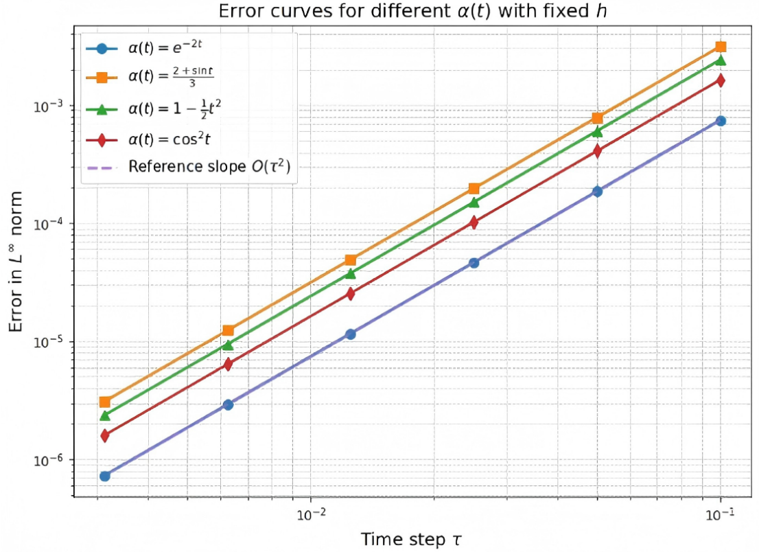
Table 1 fixes the spatial step size at h = π /500 and tests temporal steps τ from 1 / 10 to 1 / 160 . It reports the maximum error and the corresponding temporal convergence order of the compact difference scheme for four choices of α ( t ) = e 2 t , 2 + sin t 3 , 1 1 2 t 2 , cos 2 t . Figure 2 shows the error plots obtained for different values of α ( t ) with a fixed time step h = π /400 and τ ranging from 1 / 10 to 1 / 160 . These numerical results demonstrate second-order convergence in time.
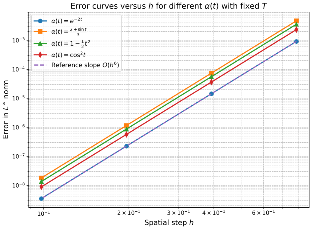
Table 2 presents the maximum error and the associated spatial convergence order of the compact difference scheme as the spatial step size varies. The observed spatial convergence order is approximately sixth order. Figure 3 presents the error plots obtained for different values of α ( t ) , with time steps h = π /4, π /8, π /16, π /32 and corresponding τ values of 1/8, 1/64, 1/512, 1/4096, respectively. Both the temporal and spatial convergence orders agree with the theoretical predictions in Theorem 3.
Example 2. 
Let L = π , T = 10 . The exact solution is u ( x , t ) = ( t 3 + 3 t 2 + 1 ) sin x . From this, the source term and the initial condition are determined as
f ( x , t ) = 6 t 3 α ( t ) Γ ( 4 α ( t ) ) + 6 t 2 α ( t ) Γ ( 3 α ( t ) ) + t 3 + 3 t 2 + 1 sin x ,
φ ( x ) = sin x .
Compared with Example 1, the errors and convergence orders for different α ( t ) under larger time intervals are presented in Table 3 and Table 4 in Example 2. The results show good agreement between the theoretical and numerical findings.
Example 3. 
Let L = π , T = 1 , u ( x , t ) = ( t 3 + 3 t 2 + 1 ) sin x . The source term and the initial condition are determined as
f ( x , t ) = 6 t 3 α ( t ) Γ ( 4 α ( t ) ) + 6 t 2 α ( t ) Γ ( 3 α ( t ) ) + t 3 + 3 t 2 + 1 sin x ,
φ ( x ) = sin x .
This example is intended to compare the errors with the scheme (3.36)–(3.38) which reach fourth order in space in [10]. Then, the errors and convergence orders for different α ( t ) are presented in Table 5. Acoording to the results, although the computational CPU cost is basically comparable to scheme (3.36)–(3.38), the error of scheme (11)–(13) is smaller, indicating that our scheme outperforms the scheme in [10] in spatial accuracy.

6. Conclusions

This work presents a compact finite difference discretization for variable-order time-fractional sub-diffusion equations. Temporal discretization employs the L2-1 σ approximation yielding second-order accuracy, while spatial discretization utilizes a novel operator A achieving sixth-order approximation. A priori estimates are derived via energy analysis, establishing unconditional stability and convergence. Numerical experiments confirm the theoretical convergence rate of O ( τ 2 + h 6 ) . In contrast to prevailing methods restricted to fourth-order spatial accuracy, this approach offers enhanced capabilities for high-resolution modeling of variable-order anomalous diffusion. The proposed sixth-order spatial operator shows promise for broader applications in variable-order fractional PDEs. In future work, we may further investigate extending this problem to two-dimensional and three-dimensional spaces, developing fast solution algorithms for higher-order schemes such as multigrid and FFT-based approaches to improve computational efficiency, and incorporating adaptive time stepping to automatically adjust the temporal resolution based on solution variations.

Author Contributions

Conceptualization, Y.B. and X.Z.; methodology, Y.B. and X.Z.; software, Y.W.; validation, Y.B. and X.Z.; formal analysis, Y.B.; investigation, Y.B.; resources, Y.J.; data curation, Y.B.; writing—original draft preparation, Y.B.; writing—review and editing, X.Z., Y.W. and Y.J.; visualization, Y.W.; supervision, Y.J.; project administration, Y.J.; funding acquisition, Y.J. All authors have read and agreed to the published version of the manuscript.

Funding

This research was funded by the Natural Science Foundation of Jilin Province No. YDZJ202501ZYTS584.

Data Availability Statement

All the data were computed using our algorithm.

Conflicts of Interest

The authors declare that they do not have any conflicts of interest.

References

  1. Samko, S.G.; Ross, B. Integration and differentiation to a variable fractional order. Integral Transform. Spec. Funct. 1993, 1, 277–300. [Google Scholar]
  2. Lorenzo, C.F.; Hartley, T.T. Variable order and distributed order fractional operators. Nonlinear Dyn. 2002, 29, 57–98. [Google Scholar] [CrossRef]
  3. Coimbra, C.F.M. Mechanics with variable-order differential operators. Ann. Phys. 2003, 12, 692–703. [Google Scholar]
  4. Sun, H.G.; Chen, W.; Wei, H.; Chen, Y.Q. A comparative study of constant-order and variable-order fractional models in characterizing memory property of systems. Eur. Phys. J. Spec. Top. 2011, 193, 185–192. [Google Scholar] [CrossRef]
  5. Patnaik, S.; Hollkamp, J.P.; Semperlotti, F. Applications of variable-order fractional operators: A review. Proc. R. Soc. A 2020, 476, 20190498. [Google Scholar] [CrossRef]
  6. Sun, H.G.; Chen, W.; Chen, Y.Q. Variable-order fractional differential operators in anomalous diffusion modeling. Physica A 2009, 388, 4586–4592. [Google Scholar]
  7. Sibatov, R.T.; L‘vov, P.E.; Sun, H.G. Variable-order fractional diffusion: Physical interpretation and simulation within the multiple trapping model. Appl. Math. Comput. 2024, 482, 128960. [Google Scholar] [CrossRef]
  8. Chen, C.M.; Liu, F.; Burrage, K.; Chen, Y. Numerical methods for the variable-order anomalous subdiffusion equation. J. Comput. Appl. Math. 2012, 277, 345–366. [Google Scholar]
  9. Zhao, X.; Sun, Z.Z.; Karniadakis, G.E. Second-order approximations for variable-order fractional derivatives. SIAM J. Numer. Anal. 2015, 53, 933–955. [Google Scholar]
  10. Du, R.; Sun, Z.Z.; Wang, H. Temporal second order difference schemes for the multi-dimensional variable-order time fractional sub-diffusion equations. Comput. Math. Appl. 2020, 79, 2952–2972. [Google Scholar] [CrossRef]
  11. Cao, J.; Qiu, Y.; Song, G. A compact finite difference scheme for variable order subdiffusion equation. Commun. Nonlinear Sci. Numer. Simul. 2017, 48, 140–149. [Google Scholar] [CrossRef]
  12. Zhang, X.; Bo, Y.; Jin, Y. A temporal second-order difference scheme for variable-order-time fractional-sub-diffusion equations of the fourth order. Fractal Fract. 2024, 8, 112. [Google Scholar] [CrossRef]
  13. Zhang, J.L.; Fang, Z.W.; Sun, H.W. Fast second-order evaluation for variable-order Caputo fractional derivative with applications to fractional sub-diffusion equations. Numer. Math. Theory Methods Appl. 2022, 15, 200–226. [Google Scholar] [CrossRef]
  14. Quintana-Murillo, J.; Yuste, S.B. An adaptive difference method for variable-order fractional-time subdiffusion equations. Mediterr. J. Math. 2024, 21, 145. [Google Scholar] [CrossRef]
  15. Kumar, V.; Srivastava, N.; Rajput, P. Higher order stable numerical algorithm for the variable order time-fractional sub-diffusion equation. Iran. J. Sci. 2025, 49, 369–381. [Google Scholar]
  16. Zhou, S.; Meng, F.; Feng, Q.; Dong, L. A spatial sixth order finite difference scheme for time fractional sub-diffusion equation with variable coefficient. IAENG Int. J. Appl. Math. 2017, 47, 175–181. [Google Scholar]
  17. Roul, P.; Goura, V.M.K.P.; Cavoretto, R. A numerical technique based on b-spline for a class of time-fractional diffusion equation. Comput. Appl. Math. 2020, 39, 1–9. [Google Scholar]
  18. Zhang, X.; Feng, Y.; Luo, Z.; Liu, J. A spatial sixth-order numerical scheme for solving fractional partial differential equation. Appl. Math. Lett. 2025, 159, 109265. [Google Scholar] [CrossRef]
  19. Dehghan, M.; Safarpoor, M. Sixth-order non-uniform combined compact difference scheme for multi-term time fractional diffusion-wave equation. Appl. Numer. Math. 2018, 131, 72–94. [Google Scholar]
  20. Soori, Z.; Aminataei, A. Effect of the nodes near boundary points on the stability analysis of sixth-order compact finite difference ADI scheme for the two-dimensional time fractional diffusion-wave equation. Trans. A. Razmadze Math. Inst. 2018, 172, 582–605. [Google Scholar]
  21. Lu, X.; Zhang, C.; Xue, H.; Zhong, B. A hybrid ESA-CCD method for variable-order time-fractional diffusion equations. J. Appl. Math. Phys. 2024, 12, 3053–3065. [Google Scholar] [CrossRef]
  22. Zhang, X.; Zhang, Y.R.; Jin, Q.Z.; Jin, Y.F. Two sixth-order, L convergent, and stable compact difference schemes for the generalized Rosenau-KdV-RLW equation. J. Comput. Appl. Math. 2025, 459, 116382. [Google Scholar] [CrossRef]
  23. Sun, Z. The Method of Order Reduction and Its Application to the Numerical Solutions of Partial Differential Equations; Science Press: Beijing, China, 2009. [Google Scholar]
  24. Lax, P.D.; Richtmyer, R.D. Survey of the stability of linear finite difference equations. Commun. Pure Appl. Math. 1956, 9, 267–293. [Google Scholar] [CrossRef]
Figure 1. The flowchart of the scheme.
Fractalfract 10 00347 g001
Figure 2. The time error of scheme (11)–(13).
Fractalfract 10 00347 g002
Figure 3. The spatial error of scheme (11)–(13).
Fractalfract 10 00347 g003
Table 1. Maximum error and convergence order in time for h = π / 500 in Example 1.
α ( t ) τ E ( h , τ ) order τ
e 2 t 1/107.440164  × 10 4
1/201.859439  × 10 4 2.0005
1/404.648149  × 10 5 2.0001
1/801.162006  × 10 5 2.0000
1/1602.904990  × 10 6 2.0000
2 + sin t 3 1/103.137139  × 10 3
1/207.861705  × 10 4 1.9965
1/401.967905  × 10 4 1.9982
1/804.922923  × 10 5 1.9991
1/1601.231129  × 10 5 1.9995
1 1 2 t 2 1/102.416212  × 10 3
1/206.027455  × 10 4 2.0031
1/401.506062  × 10 4 2.0008
1/803.764664  × 10 5 2.0002
1/1609.411359  × 10 6 2.0000
cos 2 t 1/101.635768  × 10 3
1/204.082210  × 10 4 2.0025
1/401.020122  × 10 4 2.0006
1/802.550040  × 10 5 2.0002
1/1606.374932  × 10 6 2.0000
Table 2. Maximum error and convergence order in space in Example 1.
α ( t ) h τ E ( h , τ ) order h
e 2 t π / 5 1 / 10 6.456786  × 10 4
π / 10 1 / 80 1.062061  × 10 5 5.9259
π / 20 1 / 640 1.660152  × 10 7 5.9994
π / 40 1 / 5120 2.594223  × 10 9 5.9999
2 + sin t 3 π / 5 1 / 10 2.927842  × 10 3
π / 10 1 / 80 4.832728  × 10 5 5.9209
π / 20 1 / 640 7.556097  × 10 7 5.9991
π / 40 1 / 5120 1.180722  × 10 8 5.9999
1 1 2 t 2 π / 5 1 / 10 2.242229  × 10 3
π / 10 1 / 80 3.674701  × 10 5 5.9312
π / 20 1 / 640 5.742105  × 10 7 5.9999
π / 40 1 / 5120 8.972250  × 10 9 6.0000
cos 2 t π / 5 1 / 10 1.497095  × 10 3
π / 10 1 / 80 2.455433  × 10 5 5.9300
π / 20 1 / 640 3.837140  × 10 7 5.9998
π / 40 1 / 5120 5.995743  × 10 9 5.9999
Table 3. Maximum error and convergence order in time for h = π / 400 in Example 2.
α ( t ) τ E ( h , τ ) order τ
e t 1/103.800289  × 10 6
1/209.485177  × 10 7 2.0024
1/402.363681  × 10 7 2.0046
1/805.773427  × 10 8 2.0335
1/1601.352146  × 10 8 2.0942
2 + sin t 4 1/104.076449  × 10 2
1/201.016144  × 10 2 2.0042
1/402.534504  × 10 3 2.0033
1/806.325004  × 10 4 2.0026
1/1601.579119  × 10 4 2.0019
cos 2 t 1/106.154543  × 10 2
1/201.534364  × 10 2 2.0040
1/403.828890  × 10 3 2.0026
1/809.558281  × 10 4 2.0021
1/1602.386611  × 10 4 2.0018
Table 4. Maximum error and convergence order in space in Example 2.
α ( t ) h τ E ( h , τ ) order h
e t π / 5 1 / 10 1.185484  × 10 2
π / 10 1 / 80 1.913502  × 10 4 5.9531
π / 20 1 / 640 2.976471  × 10 6 6.0065
π / 40 1 / 5120 4.641652  × 10 8 6.0028
2 + sin t 4 π / 5 1 / 10 2.406124  × 10 2
π / 10 1 / 80 3.950973  × 10 4 5.9284
π / 20 1 / 640 6.159273  × 10 6 6.0033
π / 40 1 / 5120 9.607447  × 10 8 6.0025
cos 2 t π / 5 1 / 10 4.165475  × 10 2
π / 10 1 / 80 6.835123  × 10 4 5.9294
π / 20 1 / 640 1.065059  × 10 5 6.0040
π / 40 1 / 5120 1.781000  × 10 7 5.9021
Table 5. Maximum errors and convergence orders in space for τ = 1/20,000.
Scheme (3.36)–(3.38) in 1D in [10]Scheme (11)–(13)
α ( t ) h E ( h , τ ) order h CPU ( s ) E ( h , τ ) order h CPU ( s )
cos 2 t π / 4 3.499628 × 10 3 326.906250 1.596659 × 10 4 325.859375
π / 8 2.148933 × 10 4 4.0255 330.390625 2.426481 × 10 6 6.0400 331.640625
π / 16 1.336884 × 10 5 4.0067 335.609375 3.655043 × 10 8 6.0528 329.359375
π / 32 8.335495 × 10 7 4.0035 331.500000 5.290888 × 10 10 6.1102 334.578125
1 t 2 π / 4 4.059446 × 10 3 327.781250 1.851824 × 10 4 322.750000
π / 8 2.492359 × 10 4 4.0257 322.578125 2.815518 × 10 6 6.0394 321.734375
π / 16 1.550643 × 10 5 4.0066 324.796875 4.368609 × 10 8 6.0101 323.015625
π / 32 9.680424 × 10 7 4.0017 329.750000 6.814043 × 10 10 6.0025 339.890625
e t π / 4 3.446153 × 10 3 330.562500 1.572266 × 10 4 373.875000
π / 8 2.116102 × 10 4 4.0255 328.609375 2.389283 × 10 6 6.0401 330.687500
π / 16 1.316448 × 10 5 4.0067 329.046875 3.586260 × 10 8 6.0580 332.484375
π / 32 8.206860 × 10 7 4.0037 355.312500 6.505330 × 10 10 5.7847 335.328125
Disclaimer/Publisher’s Note: The statements, opinions and data contained in all publications are solely those of the individual author(s) and contributor(s) and not of MDPI and/or the editor(s). MDPI and/or the editor(s) disclaim responsibility for any injury to people or property resulting from any ideas, methods, instructions or products referred to in the content.