Data-Driven Event-Triggered Scheme for Model-Unknown Fractional-Order Networked Control Systems: A Parametrization Transform Method

Abstract

This paper proposes a parametrization transform method for model-unknown networked control systems by using a data-driven event-triggered scheme. The key contribution is that an easy-to-apply parametrization transform method is proposed to convert the model-based linear matrix inequality (LMI) conditions into data-driven ones. Compared with existing ones, using the proposed transform method is without requirements on the specified sizes, structures, and unknown system matrices’ positions of model-based LMI conditions. On this basis, by using Lyapunov theory and some inequality techniques, some data-driven condition are derived to guarantee stability. Without considering model dynamics, the controller gain and trigger parameters can be easily derived by learning from collecting offline data packets. Finally, an illustrative example is presented to showcase the outcomes.

1. Introduction

Fractional calculus extends the concepts of integration and differentiation from integer orders to arbitrary real or complex orders. The origins of fractional calculus date back to the 17th century, with early contributions from Liouville, Riemann, and later Caputo. Among various definitions, the Caputo fractional derivative is most commonly used in engineering applications because it allows integer-order initial conditions, which have clear physical interpretations [1,2]. This powerful mathematical framework is currently gaining ever increasing attention from scholars and researchers around the globe [3]. Unlike traditional integer-order derivatives, fractional-order derivatives possess a remarkable characteristic known as infinite memory. This means that the current state of a system depends on all its past states, a feature absent in standard calculus. Consequently, fractional-order derivatives have proven to be exceptionally effective tools for capturing the memory effects and hereditary behaviors observed in a wide range of materials and processes, including viscoelastic materials, biological systems, thermal diffusion, and financial modeling [4,5,6]. Their ability to model complex dynamics with greater fidelity makes them indispensable in many emerging scientific and engineering fields. Accordingly, investigating fractional-order networked control systems is of great theoretical and practical importance.

Recently, learning from data paradigms has garnered significant attention in the realms of computing technologies and control design [7,8,9,10,11]. A critical examination of existing data-driven transform methods reveals several common limitations. The fundamental lemma approach [8,12] assumes noise-free data, which is rarely satisfied in practice. Petersen’s lemma method [13] and the matrix S-lemma method [14] can handle bounded noise but require the model-based LMI conditions to satisfy strict structural constraints, including specific sizes, quadratic forms, or prescribed positions of unknown matrices. More recent works [15,16] relax some of these constraints, yet they still cannot accommodate advanced analysis tools such as looped functionals because these tools introduce additional state variables and integral terms that violate the required structures. Moreover, existing studies rarely quantify the conservatism reduction achieved by their methods or compare computational burdens. The central challenge lies in how to derive control laws from either offline or online input/output experimental data of model-unknown systems, for providing robust guarantees. Currently, this challenge can be addressed by employing both indirect data-driven control [17,18,19,20] and direct data-driven control [12,13,14,15,16]. The former typically involves a two-step scheme, that is, controller design immediately behind system identification. Bypassing the intermediate step system identification, the other data-driven control aims to construct control laws directly from a finite number of experimental data. This approach is more practical and applicable in real-world scenarios since it is difficult or impossible to identify a system model within finite offline data packets. Undoubtedly, the investigation of data-driven control constitutes a quite popular topic in the field of advanced control.

For data-driven control, the key point is how to transform model-based LMI conditions into data-driven ones [21]. A comparative analysis of existing transform methods reveals their respective limitations. The fundamental lemma proposed by [8] has played a crucial role in deriving many corresponding advancements [12]. However, this approach assumes noise-free data, which is rarely satisfied in practical applications, thus impeding an accurate representation of the actual system. To address this issue, a robust control method [13] has been presented based on Petersen’s lemma [22]. Nevertheless, this method requires the model-based LMI to have a specific structure where unknown matrices appear in a particular form. In addition, another robust analysis method has been developed to design controllers by proposing a matrix S-lemma [14]. In the matrix S-lemma framework, the derived model-based LMI conditions must satisfy specified sizes and quadratic constraints. To solve this problem, [15,16] developed a new transform method for establishing data-driven LMI conditions from model-based ones. However, before using this method, the unknown system matrices are required to be placed at designated positions in the model-based LMI conditions. To summarize, the prerequisite for using these existing transform methods [12,13,14,15,16] is that the model-based LMI conditions must satisfy certain specified sizes, structures, or positional requirements of unknown system matrices. This observation naturally raises the following question: Can we develop a transform method that is free from such structural requirements? Accordingly, it is a necessary and urgent task to develop a novel transform method for data-driven control. This constitutes the first motivation of this paper.

On the other hand, all the works [12,13,14,15,16] focus on classical linear feedback control. Hence, it is a natural idea to design networked control schemes, i.e., sampled-data and event-triggered control, in the context of data-driven control. Up to now, some initial works for data-driven event-triggered control have been developed [23,24,25,26,27] based on the transform method in [14]. It should be noted that these works apply the simplest quadratic Lyapunov function [23,24,25,26,27] to obtain model-based LMI conditions before designing data-driven ones. In contrast, for model-known event-triggered systems [28,29,30], more advanced analysis methods and inequality techniques, such as the looped-functional method and the reciprocally convex inequality, have been well developed, leading to significantly improved results. However, these advanced methods introduce additional state variables, integral terms, and free matrices into the model-based LMI conditions. Consequently, due to the structural limitations of existing transform methods [12,13,14,15], these improved model-based conditions cannot be converted into data-driven ones. Overall, the existing data-driven control techniques lag behind the accomplishments seen in model-based control. Clearly, there is still much room for improvement. This observation naturally leads to an interesting question: Can the developed analysis methods and inequality techniques for model-known systems, such as those in [28,29,30], be successfully applied to data-driven control? At present, few works have focused on this challenging problem. This constitutes the second motivation of this paper.

To answer the above-mentioned issues, this paper proposes a data-driven approach for designing a switching event-triggered scheme for model-unknown fractional-order networked control systems by collecting offline data packets. The main contributions of this paper are summarized as follows.

1.

A novel parametrization transform method: We present a useful parametrization transform method (Lemma 2) that converts model-based LMI conditions into data-driven ones. Unlike existing methods, our approach imposes no requirements on the specified sizes, fractional order, or positions of unknown system matrices in the original model-based LMI conditions. This flexibility is the key that enables the application of advanced analysis techniques to data-driven control.

2.

Data-driven event-triggered control design: By applying the proposed parametrization transform method together with looped-functional and Jensen’s inequality techniques, we develop two sets of data-driven LMI conditions (Theorems 3 and 4) that directly involve trigger parameters, controller gain, and offline data packets. These conditions allow the controller gain and event-triggered parameters to be solved without any knowledge of the system dynamics.

Notation. Throughout this paper, $\mathbb{N}$, ${\mathbb{R}}^n$, ${\mathbb{R}}^{n\times n}$ denote the sets of natural numbers, $n\times 1$ real vectors, and $n\times n$ real matrices. $A>0(\mathrm{or}A\ge 0)$ denotes that A is a symmetric and positive definite (or semi-definite) matrix. $A^T(\mathrm{or} A^{-1})$ stands for transpose (or inverse) of matrix A. $col\{\cdots \}$, and $\left|\right|·{\left|\right|}_p$ denotes a column vector and p-norm, $p=1,2,\infty$, of a vector or a matrix, respectively. $I$, 0 denote the identity matrix and zero matrix with appropriate dimensions, respectively. ${\left[A\right]}_{\frac{(i,j)}{(N,N)}}$ implies that matrix A is located at the $i-$, $j-$ part in a matrix with $N\times N$ parts, $1\le i,j\le N$. The other parts are zero matrices with appropriate dimensions. LMI means linear matrix inequality.

2. Problem Formulation and Preliminaries

Consider the model-unknown fractional-order networked control systems as follows:

$$\begin{array}{cc}\hfill & {}_{0}D_t^{\alpha }x\left(t\right)=Ax\left(t\right)+Bu\left(t\right)+\omega \left(t\right),\hfill \end{array}$$

where $A\in {\mathbb{R}}^{n\times n}$, $B\in {\mathbb{R}}^{n\times m}$ denote the unknown system matrices. $x\left(t\right)\in {\mathbb{R}}^n$, $u\left(t\right)\in {\mathbb{R}}^m$, $\omega \left(t\right)$ are the system state, control input, and unknown disturbance, respectively.

In the field of data-driven control [12,13,14,15,16], the state, state derivative, and disturbance are supposed to be measured. Then, instead of depending on model foreknowledge, the offline data packets can be measured $\zeta$ times to design the controller. Here, we collect data packets in the following matrices:

$${}_{0}D_t^{\alpha }X={[}_0{D}_t^{\alpha }x\left(1\right){}_{0}D_t^{\alpha }x\left(2\right)\cdots {}_{0}D_t^{\alpha }x\left(\zeta \right)]\in {\mathbb{R}}^{n\times \zeta },$$

$$X=[x\left(1\right)x\left(2\right)\cdots x\left(\zeta \right)]\in {\mathbb{R}}^{n\times \zeta },$$

$$H=[u\left(1\right)u\left(2\right)\cdots u\left(\zeta \right)]\in {\mathbb{R}}^{m\times \zeta },$$

where $i=1,\cdots ,\zeta$. Also, the unknown disturbance sequence can be set as

$$W=[\omega \left(1\right)\omega \left(2\right)\cdots \omega \left(\zeta \right)]\in {\mathbb{R}}^{n\times \zeta }.$$

Thus, we can derive that ${}_{0}D_t^{\alpha }X=AX+BH+W$.

Remark 1.

The Caputo fractional derivative is used throughout this paper, defined as ${}_{0}D_t^{\alpha }f\left(t\right)={\displaystyle \frac{1}{\Gamma (1-\alpha )}}{\int }_0^t{(t-\tau )}^{-\alpha }{f}^{\prime }\left(\tau \right)d\tau$ for $0<\alpha <1$, where $\Gamma (·)$ is the Gamma function. This definition is chosen because it allows integer-order initial conditions, which have clear physical interpretations.

Remark 2.

In practice, the fractional derivative ${}_{0}D_t^{\alpha }x\left(t\right)$ is not directly measurable. It is obtained numerically from the sampled state data X using standard approximation methods such as the Grünwald–Letnikov scheme or the Oustaloup recursive filter. The approximation errors can be absorbed into the disturbance term W, and as long as the total uncertainty satisfies the energy bound condition, the proposed method remains valid.

As pointed out in [12,13,14,15,16], the noise data is unknown but energy-limited. That is, there exists a known matrix $\Delta \in {\mathbb{R}}^{n\times n}\ge 0$ such that $W\in \mathcal{W}$, and

$$\begin{array}{c}\hfill \mathcal{W}:={WW}^T\le {\Delta \Delta }^T.\end{array}$$

(1)

Combined with the offline data packets and (1), the following set $\Gamma$ can be defined:

$$\Gamma :=\left\{\left[AB\right]:{}_{0}D_t^{\alpha }X=AX+BH+W,\left[\begin{array}{cc}I& W\end{array}\right]\left[\begin{array}{cc}-\Delta {\Delta }^T& 0\\ \ast & I\end{array}\right]\left[\begin{array}{c}I\\ W^T\end{array}\right]\le 0\right\}.$$

Assumption 1.

Matrix $\left[\begin{array}{c}X\\ H\end{array}\right]$ has full row rank.

Remark 3.

Assumption 1 is not an unverifiable assumption but rather a condition that can be checked directly from the collected data. If the condition fails, additional data points can be collected until it holds. This is a standard persistency of excitation condition in data-driven control, ensuring that the collected data is sufficiently rich to excite all dynamic modes of the system.

Owing to $W{=}_0{D}_t^{\alpha }X-AX-BH$, the set Γ can be rewritten as

$$\begin{array}{cc}\hfill \Gamma & :=\left\{\left[AB\right]:{\left[\begin{array}{c}I\\ A^T\\ B^T\end{array}\right]}^T\left[\begin{array}{cc}{N}_1& N_2^T\\ N_2& N_3\end{array}\right]\left[\begin{array}{c}I\\ A^T\\ B^T\end{array}\right]\le 0\right\}\hfill \\ \hfill & :=\left\{\left[AB\right]=Z^T:N_1+N_2^{T}Z+Z^T{N}_2+Z^T{N}_{3}Z\le 0\right\}\hfill \\ \hfill & :=\left\{\left[AB\right]=Z^T:{(Z-\xi )}^T{N}_3(Z-\xi )\le Q\right\}.\hfill \end{array}$$

(2)

where $\xi =-N_3^{-1}{N}_2$, $Q=N_2^T{N}_3^{-1}{N}_2-N_1$, and

$\left[\begin{array}{cc}{N}_1& N_2^T\\ N_2& N_3\end{array}\right]=\left[\begin{array}{cc}{}_{0}D_t^{\alpha }{X}_0{D}_t^{\alpha }{X}^T-\Delta {\Delta }^T& {-}_0{D}_t^{\alpha }X{\left[\begin{array}{c}X\\ H\end{array}\right]}^T\\ \ast & \left[\begin{array}{c}X\\ H\end{array}\right]{\left[\begin{array}{c}X\\ H\end{array}\right]}^T\end{array}\right]$.

Remark 4.

The matrices $N_1$, $N_2$, $N_3$, ξ, and Q are computed directly from the collected offline data packets X, H, and ${}_{0}D_t^{\alpha }X$, together with the noise bound Δ. Therefore, the set Γ provides a data-driven characterization of all possible system matrices $\left[AB\right]$ that are consistent with the noisy data.

Lemma 1

([13]). Under Assumption 1, it yields (1) $N_3>0$, $Q\ge 0$; (2) Define

$$\Theta :=\left\{{(\xi +N_3^{-1/2}{\rm Y}{Q}^{1/2})}^T\right\},$$

and it yields $\Theta =\Gamma$ for some matrix ${\rm Y}$ with $\left|\right|{\rm Y}\left|\right|\le 1$.

Remark 5.

Lemma 1 provides an explicit parametrization of the set Γ. When $\Delta =0$ (noise-free case), we have $Q=0$, and the set Θ collapses to the single point ${\xi }^T$. When $\Delta >0$ (noisy case), the uncertainty matrix ${\rm Y}$ captures all possible system matrices consistent with the data.

Next, an important lemma is presented as follows.

Lemma 2.

For unknown system matrices $A\in {\mathbb{R}}^{n\times n}$, $B\in {\mathbb{R}}^{n\times m}$, and matrices $U\in {\mathbb{R}}^{n\times n}$, $G\in {\mathbb{R}}^{m\times n}$, and $Z^T=\left[AB\right]\in \Xi$, the following conditions are true if and only if $Z=\xi +N_3^{-1/2}{\rm Y}{Q}^{1/2}$ with some matrix ${\rm Y}$ with ${{\rm Y}}^T{\rm Y}\le I$ such that

$$\begin{array}{cc}\hfill \mathit{Sym}\left\{{[AU+BG]}_{\frac{(i,j)}{(N,N)}}\right\}& =\mathit{Sym}\left\{{\left[{\xi }^T\left[\begin{array}{c}U\\ G\end{array}\right]\right]}_{\frac{(i,j)}{(N,N)}}\right\}\hfill \end{array}$$

$$+\mathit{Sym}\left\{{\left[Q^{1/2}\right]}_{\frac{(i,1)}{(N,1)}}{{\rm Y}}^T{\left[N_3^{-1/2}\left[\begin{array}{c}U\\ G\end{array}\right]\right]}_{\frac{(1,j)}{(1,N)}}\right\},$$

(3)

$$\begin{array}{cc}\hfill \mathit{Sym}\left\{{\left[BG\right]}_{\frac{(i,j)}{(N,N)}}\right\}& =\mathit{Sym}\left\{{\left[{\xi }^T\left[\begin{array}{c}0\\ I\end{array}\right]G\right]}_{\frac{(i,j)}{(N,N)}}\right\}\hfill \end{array}$$

$$+\mathit{Sym}\left\{{\left[Q^{1/2}\right]}_{\frac{(i,1)}{(N,1)}}{{\rm Y}}^T{\left[N_3^{-1/2}\left[\begin{array}{c}0\\ I\end{array}\right]G\right]}_{\frac{(1,j)}{(1,N)}}\right\},$$

(4)

where $1\le i,j\le N$.

Proof of Lemma 2.

Denote $AU+BG=\left[AB\right]\left[\begin{array}{c}U\\ G\end{array}\right]=Z^T\left[\begin{array}{c}U\\ G\end{array}\right]$. For $Z=\xi +N_3^{-1/2}{\rm Y}{Q}^{1/2}$ with ${{\rm Y}}^T{\rm Y}\le I$, it has $AU+BG={(\xi +N_3^{-1/2}{\rm Y}{Q}^{1/2})}^T\left[\begin{array}{c}U\\ G\end{array}\right]$. Then, one can obtain

$$\begin{array}{cc}\hfill \mathrm{Sym}\left\{{[AU+BG]}_{\frac{(i,j)}{(N,N)}}\right\}& =\mathrm{Sym}\left\{{\left[{\xi }^T\left[\begin{array}{c}U\\ G\end{array}\right]\right]}_{\frac{(i,j)}{(N,N)}}\right\}\hfill \end{array}$$

$$\begin{array}{c}\hfill +\mathrm{Sym}\left\{{\left[Q^{1/2}{{\rm Y}}^T{N}_3^{-1/2}\left[\begin{array}{c}U\\ G\end{array}\right]\right]}_{\frac{(i,j)}{(N,N)}}\right\}.\end{array}$$

(5)

It can be seen that

$$\begin{array}{cc}\hfill {\left[Q^{1/2}{{\rm Y}}^T{N}_3^{-1/2}\left[\begin{array}{c}U\\ G\end{array}\right]\right]}_{\frac{(i,j)}{(N,N)}}& =\left[\begin{array}{c}\stackrel{(i-1)\times 1\mathrm{parts}}{\overbrace{\begin{array}{|c|}\hline \begin{array}{c}0\\ ⋮\\ 0\end{array}\\ \hline\end{array}}}\\ Q^{1/2}\\ \underset{(N-i)\times 1\mathrm{parts}}{\underbrace{\begin{array}{|c|}\hline \begin{array}{c}0\\ ⋮\\ 0\end{array}\\ \hline\end{array}}}\end{array}\right]{{\rm Y}}^T\hfill \\ & \times \left[\stackrel{1\times (j-1)\mathrm{parts}}{\overbrace{\begin{array}{|c|}\hline 0\cdots 0\\ \hline\end{array}}}{N}_3^{-1/2}\left[\begin{array}{c}U\\ G\end{array}\right]\stackrel{1\times (N-j)\mathrm{parts}}{\overbrace{\begin{array}{|c|}\hline 0\cdots 0\\ \hline\end{array}}}\right]\hfill \end{array}$$

$$={\left[Q^{1/2}\right]}_{\frac{(i,1)}{(N,1)}}{\mathrm{Y}}^T{\left[N_3^{-1/2}\left[\begin{array}{c}U\\ G\end{array}\right]\right]}_{\frac{(1,\mathrm{j})}{(1,\mathrm{N})}},$$

(6)

where 0 denotes a zero matrix with appropriate dimensions.    □

Remark 6.

Lemma 2 is the core of the proposed parametrization transform method. It expresses terms containing the unknown matrices A and B in terms of data-driven quantities ξ, $N_3$, and Q, plus the uncertainty matrix ${\rm Y}$. In the noise-free case ($Q=0$), the ${\rm Y}$-dependent terms vanish, yielding exact data-driven expressions. This lemma serves as the bridge that enables the conversion of model-based LMI conditions into data-driven ones.

In view of (5)–(6), one can obtain condition (3). Also, $BG=\left[AB\right]\left[\begin{array}{c}0\\ I\end{array}\right]G=Z^T\left[\begin{array}{c}0\\ I\end{array}\right]G$. By using a similar method, it yields (4) directly.

On the other hand, consider the control input is designed as follows: $u\left(t\right)=Kx\left(t_k\right),t\in [t_k,t_{k+1}),$ where $K\in {\mathbb{R}}^{m\times n}$ denotes the controller gain. The corresponding switching event-triggered scheme [31] is formulated as

$$t_{k+1}=inf\{t\ge t_k+h_k|{\eta }^T\left(t\right)\Omega \eta \left(t\right)\le \lambda x^T\left(t\right)\Omega x\left(t\right)\},$$

(7)

where $\eta \left(t\right)=x\left(t_k\right)-x\left(t\right)$, $\lambda >0$ is the threshold parameter, $\Omega >0$ is the trigger matrix, and $[t_k,t_k+h_k)$ denotes the rest interval of (7) with $0<\underline{h}\le h_k\le \overline{h}$.

In view of Lemma 2 and (7) and considering $\omega \left(t\right)=0$, one can obtain

$$\begin{array}{c}\hfill {}_{t_k}D_t^{\alpha }x\left(t\right)=Ax\left(t\right)+Bu\left(t\right).\end{array}$$

(8)

Remark 7.

The switching event-triggered scheme works as follows. After each triggering instant $t_k$, there is a mandatory waiting period $h_k$ during which no event is checked. This waiting period prevents Zeno behavior (infinitely many triggers in finite time). After the waiting period, the scheme continuously monitors the condition ${\eta }^T\left(t\right)\Omega \eta \left(t\right)\le \lambda x^T\left(t\right)\Omega x\left(t\right)$. When this condition is satisfied, a new trigger instant $t_{k+1}$ is generated and the control input is updated. The event condition ensures that the sampling error $\eta \left(t\right)=x\left(t_k\right)-x\left(t\right)$ remains small relative to the current state.

Remark 8.

Equation (8) represents the nominal closed-loop system without disturbance. The disturbance $\omega \left(t\right)$ was introduced earlier to motivate the data-driven transformation method and to define the parameter set Γ in Lemma 1. However, once the transformation is established and the data-driven conditions are derived, we focus on the nominal system for stability analysis, which is a common two-step procedure in data-driven control.

For the sake of convenience in notation, we denote ${}_{t_k}D_t^{\alpha }$ by $D_t^{\alpha }$.

3. Main Results

3.1. Model-Based Stability Analysis

Theorem 1.

For given scalars $\lambda >0$, $\overline{h}\ge \underline{h}>0$, and control gain K, system (8) is globally asymptotically stable if there exist $n\times n$ matrices $P>0$, $R>0$, $\Omega >0$, a $2n\times 2n$ matrix $\mathit{X}=\left[\begin{array}{cc}{\displaystyle \frac{X+X^T}{2}}& -X+X_1\\ \ast & -X_1-X_1^T+{\displaystyle \frac{X+X^T}{2}}\end{array}\right]$, and $n\times n$ matrices $P_1$, $P_2$, $P_3$, $P_4$, such that the following LMIs (9)–(11) are satisfied for $h_k\in \{\underline{h},\overline{h}\}$:

$$\varphi \left(h_k\right)<0,$$

(9)

$$\phi \left(h_k\right)<0,$$

(10)

$$\Xi <0,$$

(11)

where

• ${\varphi }_{11}=-\frac{X+X^T}{2}+P_1^T(A+BK)+{(A+BK)}^T{P}_1$;
• ${\varphi }_{12}=P-P_1^T+{(A+BK)}^T{P}_2$;
• ${\varphi }_{13}=X-X_1$;
• ${\varphi }_{14}=-h_k{P}_1^{T}BK$;
• ${\varphi }_{22}=-P_2-P_2^T$;
• ${\varphi }_{24}=-h_k{P}_2^{T}BK$;
• ${\varphi }_{33}=X_1+X_1^T-\frac{X+X^T}{2}$;
• ${\varphi }_{44}=-h_{k}R$;
• ${\phi }_{11}={\varphi }_{11}$;
• ${\phi }_{12}=h_k\frac{X+X^T}{2}+{\varphi }_{12}$;
• ${\phi }_{13}={\varphi }_{13}$;
• ${\phi }_{22}=h_{k}R+{\varphi }_{22}$;
• ${\phi }_{23}=h_k(-X+X_1)$;
• ${\phi }_{33}={\varphi }_{33}$;
• ${\Xi }_{11}=P_3^{T}A+A^T{P}_3+\lambda \Omega -\Omega$;
• ${\Xi }_{12}=P+A^T{P}_4-P_3^T$;
• ${\Xi }_{13}=P_3^{T}BK+\Omega$;
• ${\Xi }_{22}=-P_4-P_4^T$;
• ${\Xi }_{23}=P_4^{T}BK$;
• ${\Xi }_{33}=-\Omega$.

Other blocks are zero matrices. That is, the solutions of closed-loop system (8) converge asymptotically to the origin by using the switching event-triggered mechanism.

Proof of Theorem 1.

Consider the following looped functional as

$$V\left(t\right)={\displaystyle \sum _{i=1}^3}{V}_i\left(t\right),$$

and

$$V_1\left(t\right)=x^T\left(t\right)Px\left(t\right),$$

$$V_2\left(t\right)=(t_{k+1}-t){\int }_{t_k}^t{D}_t^{\alpha }{x}^T\left(s\right)R{D}_t^{\alpha }x\left(s\right)ds,$$

$$V_3\left(t\right)=(t_{k+1}-t){\left[\begin{array}{c}x\left(t\right)\\ x\left(t_k\right)\end{array}\right]}^T\mathbf{X}\left[\begin{array}{c}x\left(t\right)\\ x\left(t_k\right)\end{array}\right],$$

where $\mathbf{X}=\left[\begin{array}{cc}{\displaystyle \frac{X+X^T}{2}}& -X+X_1\\ \ast & -X_1-X_1^T+{\displaystyle \frac{X+X^T}{2}}\end{array}\right]$.

Differentiating $V_i\left(t\right)$, $i=1,2,3$ along the trajectories of system (8), one has

$$D_t^{\alpha }{V}_1\left(t\right)\le 2x^T\left(t\right)P{D}_t^{\alpha }x\left(t\right),$$

$$D_t^{\alpha }{V}_2\left(t\right)\le (t_{k+1}-t)D_t^{\alpha }{x}^T\left(t\right)R{D}_t^{\alpha }x\left(t\right)-{\int }_{t_k}^t{D}_t^{\alpha }{x}^T\left(s\right)R{D}_t^{\alpha }x\left(s\right)ds,$$

$$D_t^{\alpha }{V}_3\left(t\right)\le -{\left[\begin{array}{c}x\left(t\right)\\ x\left(t_k\right)\end{array}\right]}^T\mathbf{X}\left[\begin{array}{c}x\left(t\right)\\ x\left(t_k\right)\end{array}\right]+2(t_{k+1}-t){\left[\begin{array}{c}x\left(t\right)\\ x\left(t_k\right)\end{array}\right]}^T\mathbf{X}\left[\begin{array}{c}{D}_t^{\alpha }x\left(t\right)\\ 0\end{array}\right].$$

The following proof consists of two parts.

Part I: If $t\in [t_k,t_k+h_k)$, $V\left(t\right)={\sum }_{i=1}^3{V}_i\left(t\right)$. Using Jensen’s inequality, it yields

$$-{\int }_{t_k}^t{D}_t^{\alpha }{x}^T\left(s\right)R{D}_t^{\alpha }x\left(s\right)ds\le -(t-t_k){\nu }_1^{T}R{\nu }_1,$$

where ${\upsilon }_1=\frac{1}{t-t_k}{\int }_{t_k}^t{D}_t^{\alpha }x\left(s\right)ds$. Also, for matrices $P_1$, $P_2$, it has

$$0=2[x^T\left(t\right)P_1^T+D_t^{\alpha }{x}^T\left(t\right)P_2^T][(A+BK)x\left(t\right)-(t-t_k)BK{\nu }_1-D_t^{\alpha }x\left(t\right)].$$

Denote ${\eta }_1\left(t\right)=\mathrm{col}\{x\left(t\right),D_t^{\alpha }x\left(t\right),x\left(t_k\right),{\nu }_1\left(t\right)\}$, ${\eta }_2\left(t\right)=\mathrm{col}\{x\left(t\right),D_t^{\alpha }x\left(t\right),x\left(t_k\right)\}$. In view of the above analysis, it yields

$$D_t^{\alpha }V\left(t\right)\le {\displaystyle \frac{t-t_k}{h_k}}{\eta }_1^T\left(t\right)\varphi \left(h_k\right){\eta }_1\left(t\right)+{\displaystyle \frac{t_{k+1}-t}{h_k}}{\eta }_2^T\left(t\right)\phi \left(h_k\right){\eta }_2\left(t\right).$$

For $\underline{h}\le h_k\le \overline{h}$, $\varphi \left(h_k\right)<0$ and $\phi \left(h_k\right)<0$ hold by the inequalities $\varphi \left(\underline{h}\right)<0$, $\varphi \left(\overline{h}\right)<0$, $\phi \left(\underline{h}\right)<0$ and $\phi \left(\overline{h}\right)<0$, which can be guaranteed by conditions (9)–(10) and the convex combination technique. Thus, it yields $D_t^{\alpha }V\left(t\right)<0,t\in [t_k,t_k+h_k).$ Part II: If $t\in [t_k+h_k,t_{k+1})$, $V\left(t\right)=V_1\left(t\right)$. For matrices $P_3$, $P_4$, it has

$$0=2[x^T\left(t\right)P_3^T+D_t^{\alpha }{x}^T\left(t\right)P_4^T][Ax\left(t\right)+BKx\left(t_k\right)-D_t^{\alpha }x\left(t\right)].$$

Then, combined with trigger condition (7), one has $D_t^{\alpha }V\left(t\right)\le {\eta }_3^T\left(t\right)\Xi {\eta }_3\left(t\right),$ where ${\eta }_3\left(t\right)=\mathrm{col}\{x\left(t\right),D_t^{\alpha }x\left(t\right),x\left(t_k\right)\}$. Based on condition (11), it yields

$$D_t^{\alpha }V\left(t\right)<0,t\in [t_k+h_k,t_{k+1}).$$

Then, one has

$$D_t^{\alpha }V\left(t\right)<0,t\in [t_k,t_{k+1}).$$

By using hybrid Lyapunov theories [28], the solutions of closed-loop system (8) converge asymptotically to the origin by using the switching event-triggered mechanism.    □

Theorem 2.

For given scalars $\lambda >0$, $\overline{h}\ge \underline{h}>0$, θ, ρ, σ, there exist $n\times n$ matrices $\tilde{P}>0$, $\tilde{R}>0$, $\tilde{\Omega }>0$, a $2n\times 2n$ matrix $\tilde{\mathit{X}}=\left[\begin{array}{cc}{\displaystyle \frac{\tilde{X}+{\tilde{X}}^T}{2}}& -\tilde{X}+{\tilde{X}}_1\\ \ast & -{\tilde{X}}_1-{\tilde{X}}_1^T+{\displaystyle \frac{\tilde{X}+{\tilde{X}}^T}{2}}\end{array}\right]$, an $n\times n$ matrix U, and an $m\times n$ matrix G, such that the following LMIs (12)–(14) are satisfied for $h_k\in \{\underline{h},\overline{h}\}$:

$$\tilde{\varphi }\left(h_k\right)<0,$$

(12)

$$\tilde{\phi }\left(h_k\right)<0,$$

(13)

$$\tilde{\Xi }<0,$$

(14)

where

• ${\tilde{\varphi }}_{11}=-\frac{\tilde{X}+{\tilde{X}}^T}{2}+AU+BG+U^T{A}^T+G^T{B}^T$;
• ${\tilde{\varphi }}_{12}=\tilde{P}-U+\theta (U^T{A}^T+G^T{B}^T)$;
• ${\tilde{\varphi }}_{13}=\tilde{X}-{\tilde{X}}_1$;
• ${\tilde{\varphi }}_{14}=-h_{k}BG$;
• ${\tilde{\varphi }}_{22}=-\theta U-\theta U^T$;
• ${\tilde{\varphi }}_{24}=-h_k\theta BG$;
• ${\tilde{\varphi }}_{33}={\tilde{X}}_1+{\tilde{X}}_1^T-\frac{\tilde{X}+{\tilde{X}}^T}{2}$;
• ${\tilde{\varphi }}_{44}=-h_k\tilde{R}$;
• ${\tilde{\phi }}_{11}={\tilde{\varphi }}_{11}$;
• ${\tilde{\phi }}_{12}=h_k\frac{\tilde{X}+{\tilde{X}}^T}{2}+{\tilde{\varphi }}_{12}$;
• ${\tilde{\phi }}_{13}={\tilde{\varphi }}_{13}$;
• ${\tilde{\phi }}_{22}=h_k\tilde{R}+{\tilde{\varphi }}_{22}$;
• ${\tilde{\phi }}_{23}=h_k(-\tilde{X}+{\tilde{X}}_1)$;
• ${\tilde{\phi }}_{33}={\tilde{\varphi }}_{33}$;
• ${\tilde{\Xi }}_{11}=\rho AU+\rho U^T{A}^T+\lambda \tilde{\Omega }-\tilde{\Omega }$;
• ${\tilde{\Xi }}_{12}=\tilde{P}+\sigma U^T{A}^T-\rho U$;
• ${\tilde{\Xi }}_{13}=\rho BG+\tilde{\Omega }$;
• ${\tilde{\Xi }}_{22}=-\sigma U-\sigma U^T$;
• ${\tilde{\Xi }}_{23}=\sigma BG$;
• ${\tilde{\Xi }}_{33}=-\tilde{\Omega }$.

Other blocks are zero matrices. That is, the solutions of the closed-loop system (8) converge asymptotically to the origin by using the switching event-triggered mechanism. In addition, the controller gain K can be solved by $K=G{U}^{-1}$.

Proof of Theorem 2.

Denote $P_1=U^{-1}$, $P_2=\theta P_1$, $P_3=\rho P_1$, $P_4=\sigma P_1$, $\tilde{P}=U^{T}PU$, $\tilde{R}=U^{T}RU$, $\tilde{X}=U^{T}XU$, ${\tilde{X}}_1=U^T{X}_{1}U$, ${\zeta }_a=\mathrm{diag}\{U,U,U,U\}$, and ${\zeta }_b=\mathrm{diag}\{U,U,U\}$. Premultiply and postmultiply (9) by ${\zeta }_a^T$ and ${\zeta }_a$, (10) by ${\zeta }_b^T$ and ${\zeta }_b$, and (11) by ${\zeta }_b^T$ and ${\zeta }_b$, respectively. Then, by using Schur complements, one can obtain (12)–(14).    □

Remark 9.

Theorems 1 and 2 are model-based results presented as theoretical templates. They assume knowledge of the system matrices A and B and serve as the foundation for the data-driven results in Theorems 3 and 4. These theorems are not meant to be applied directly when A and B are unknown; rather, they provide the structural framework that will be transformed via Lemma 2. Theorem 1 provides model-based stability conditions using the looped-functional method. The matrices P, R, and Ω are Lyapunov matrices to be solved. The matrices X and $X_1$ appear in the looped-functional $V_3\left(t\right)$ and are slack variables that help reduce conservatism. The parameters $\underline{h}$ and $\overline{h}$ define the bounds of the waiting period $h_k$. The looped-functional $V_3\left(t\right)$ depends explicitly on both the current state $x\left(t\right)$ and the last sampled state $x\left(t_k\right)$. Its coefficient $(t_{k+1}-t)$ vanishes at the next triggering instant $t_{k+1}$, which is a key property for analyzing event-triggered systems. The special block structure of $\mathit{X}$ guarantees the non-negativity of $V_3\left(t\right)$ and facilitates the application of Jensen’s inequality. Theorem 2 is the model-based counterpart of Theorem 4. Through the change of variables $P_1=U^{-1}$, $P_2=\theta P_1$, $P_3=\rho P_1$, $P_4=\sigma P_1$, and $\tilde{P}=U^{T}PU$, the bilinear matrix inequalities in Theorem 1 are converted into linear ones. This allows the controller gain K to be solved as $K=G{U}^{-1}$. The parameters θ, ρ, σ are tuning parameters that can be adjusted to improve feasibility.

3.2. Data-Driven Stability Analysis

In view of Lemma 2, Theorem 1, and Theorem 2, two data-driven control schemes can be derived as follows.

Theorem 3.

For given scalars $\lambda >0$, $\overline{h}\ge \underline{h}>0$, and control gain K, there exist $n\times n$ matrices $P>0$, $R>0$, $\Omega >0$, a $2n\times 2n$ matrix $\mathit{X}=\left[\begin{array}{cc}\frac{X+X^T}{2}& -X+X_1\\ \ast & -X_1-X_1^T+\frac{X+X^T}{2}\end{array}\right]$, and $n\times n$ matrices $P_1$, $P_2$, $P_3$, $P_4$, such that the following LMIs (15)–(17) are satisfied for $h_k\in \{\underline{h},\overline{h}\}$:

$$\widehat{\varphi }\left(h_k\right)<0,$$

(15)

$$\widehat{\phi }\left(h_k\right)<0,$$

(16)

$$\widehat{\Xi }<0,$$

(17)

where

• ${\widehat{\varphi }}_{11}=-\frac{X+X^T}{2}+P_1^T{\xi }^T\left[\begin{array}{c}I\\ K\end{array}\right]+\left[I{K}^T\right]\xi P_1$;
• ${\widehat{\varphi }}_{12}=P-P_1^T+\left[I{K}^T\right]\xi P_2$;
• ${\widehat{\varphi }}_{13}={\varphi }_{13}$;
• ${\widehat{\varphi }}_{14}=-h_k{P}_1^T{\xi }^T\left[\begin{array}{c}0\\ I\end{array}\right]K$;
• ${\widehat{\varphi }}_{22}={\varphi }_{22}$;
• ${\widehat{\varphi }}_{24}=-h_k{P}_2^T{\xi }^T\left[\begin{array}{c}0\\ I\end{array}\right]K$;
• ${\widehat{\varphi }}_{33}={\varphi }_{33}$;
• ${\widehat{\varphi }}_{44}={\varphi }_{44}$;
• ${\widehat{\phi }}_{11}={\widehat{\varphi }}_{11}$;
• ${\widehat{\phi }}_{12}=h_k\frac{X+X^T}{2}+{\widehat{\varphi }}_{12}$;
• ${\widehat{\phi }}_{13}={\widehat{\varphi }}_{13}$;
• ${\widehat{\phi }}_{22}=h_{k}R+{\widehat{\varphi }}_{22}$;
• ${\widehat{\phi }}_{23}=h_k(-X+X_1)$;
• ${\widehat{\phi }}_{33}={\widehat{\varphi }}_{33}$;
• ${\widehat{\Xi }}_{11}=P_3^T{\xi }^T\left[\begin{array}{c}I\\ 0\end{array}\right]+\left[I0\right]\xi P_3+\lambda \Omega -\Omega$;
• ${\widehat{\Xi }}_{12}=P+\left[I0\right]\xi P_4-P_3^T$;
• ${\widehat{\Xi }}_{13}=P_3^T{\xi }^T\left[\begin{array}{c}0\\ I\end{array}\right]K+\Omega$;
• ${\widehat{\Xi }}_{22}={\Xi }_{22}$;
• ${\widehat{\Xi }}_{23}=P_4^T{\xi }^T\left[\begin{array}{c}0\\ I\end{array}\right]K$;
• ${\widehat{\Xi }}_{33}={\Xi }_{33}$;
• $\xi =-N_3^{-1}{N}_2$;
  $N_2=-\left[\begin{array}{c}X\\ H\end{array}\right]D_t^{\alpha }{X}^T$;
• $N_3=\left[\begin{array}{c}X\\ H\end{array}\right]{\left[\begin{array}{c}X\\ H\end{array}\right]}^T$.

Other blocks are zero matrices. That is, the solutions of closed-loop system (8) converge asymptotically to the origin based on data-driven switching event-triggered control.

Proof of Theorem 3.

In this proof, model-based LMI conditions (12)–(14) will be transformed into data-driven cases.

Step I: Separate unknown matrices A, B from model-based LMI conditions. Then, (9) is divided into two parts, i.e.,

$$\begin{array}{cc}\hfill \varphi \left(h_k\right)& ={\widehat{\varphi }}_1\left(h_k\right)+\mathrm{Sym}\left\{{\left[P_1^T(A+BK)\right]}_{\frac{(1,1)}{(4,4)}}\right\}\hfill \\ & +\mathrm{Sym}\left\{{\left[{(A+BK)}^T{P}_2\right]}_{\frac{(1,2)}{(4,4)}}\right\}+\mathrm{Sym}\left\{{[-h_k{P}_1^{T}BK]}_{\frac{(1,4)}{(4,4)}}\right\}\hfill \\ & +\mathrm{Sym}\left\{{[-h_k{P}_2^{T}BK]}_{\frac{(2,4)}{(4,4)}}\right\}<0,\hfill \end{array}$$

where ${\widehat{\varphi }}_1\left(h_k\right)=\left[\begin{array}{cccc}-\frac{X+X^T}{2}& P-P_1^T& {\widehat{\varphi }}_{13}& 0\\ \ast & {\widehat{\varphi }}_{22}& 0& 0\\ \ast & \ast & {\widehat{\varphi }}_{33}& 0\\ \ast & \ast & \ast & {\widehat{\varphi }}_{44}\end{array}\right]$.

Step II: Equivalent parametrization. From Lemma 2, it yields

$$\begin{array}{cc}\hfill \mathrm{Sym}\left\{{\left[P_1^T(A+BK)\right]}_{\frac{(1,1)}{(4,4)}}\right\}& =\mathrm{Sym}\left\{{\left[P_1^T{\xi }^T\left[\begin{array}{c}I\\ K\end{array}\right]\right]}_{\frac{(1,1)}{(4,4)}}\right\}\hfill \\ & +\mathrm{Sym}\left\{{\left[P_1^T{Q}^{1/2}\right]}_{\frac{(1,1)}{(4,1)}}{{\rm Y}}^T{\left[N_3^{-1/2}\left[\begin{array}{c}I\\ K\end{array}\right]\right]}_{\frac{(1,1)}{(1,4)}}\right\},\hfill \end{array}$$

$$\begin{array}{cc}\hfill \mathrm{Sym}\left\{{\left[{(A+BK)}^T{P}_2\right]}_{\frac{(1,2)}{(4,4)}}\right\}& =\mathrm{Sym}\left\{{\left[P_2^T{\xi }^T\left[\begin{array}{c}I\\ K\end{array}\right]\right]}_{\frac{(2,1)}{(4,4)}}\right\}\hfill \\ & +\mathrm{Sym}\left\{{\left[P_2^T{Q}^{1/2}\right]}_{\frac{(2,1)}{(4,1)}}{{\rm Y}}^T{\left[N_3^{-1/2}\left[\begin{array}{c}I\\ K\end{array}\right]\right]}_{\frac{(1,1)}{(1,4)}}\right\},\hfill \end{array}$$

$$\begin{array}{cc}\hfill \mathrm{Sym}\left\{{[-h_k{P}_1^{T}BK]}_{\frac{(1,4)}{(4,4)}}\right\}& =\mathrm{Sym}\left\{{\left[-h_k{P}_1^T{\xi }^T\left[\begin{array}{c}0\\ I\end{array}\right]K\right]}_{\frac{(1,4)}{(4,4)}}\right\}\hfill \\ & +\mathrm{Sym}\left\{{\left[-P_1^T{Q}^{1/2}\right]}_{\frac{(1,1)}{(4,1)}}{{\rm Y}}^T{\left[h_k{N}_3^{-1/2}\left[\begin{array}{c}0\\ I\end{array}\right]K\right]}_{\frac{(1,4)}{(1,4)}}\right\},\hfill \end{array}$$

$$\begin{array}{cc}\hfill \mathrm{Sym}\left\{{[-h_k{P}_2^{T}BK]}_{\frac{(2,4)}{(4,4)}}\right\}& =\mathrm{Sym}\left\{{\left[-h_k{P}_2^T{\xi }^T\left[\begin{array}{c}0\\ I\end{array}\right]K\right]}_{\frac{(2,4)}{(4,4)}}\right\}\hfill \\ & +\mathrm{Sym}\left\{{\left[-P_2^T{Q}^{1/2}\right]}_{\frac{(2,1)}{(4,1)}}{{\rm Y}}^T{\left[h_k{N}_3^{-1/2}\left[\begin{array}{c}0\\ I\end{array}\right]K\right]}_{\frac{(1,4)}{(1,4)}}\right\}.\hfill \end{array}$$

Step III: Establish data-driven LMI conditions. From (8), owing to disturbance $w\left(t\right)=0$, it has $\Delta =0$, and $Q=N_2^T{N}_3^{-1}{N}_2-N_1=0$. Hence, from Step I–Step II, one can obtain

$$\begin{array}{cc}\hfill \varphi \left(h_k\right)& ={\widehat{\varphi }}_1\left(h_k\right)+\mathrm{Sym}\left\{{\left[P_1^T{\xi }^T\left[\begin{array}{c}I\\ K\end{array}\right]\right]}_{\frac{(1,1)}{(4,4)}}+{\left[P_2^T{\xi }^T\left[\begin{array}{c}I\\ K\end{array}\right]\right]}_{\frac{(2,1)}{(4,4)}}\right.\hfill \\ & +\left.{\left[-h_k{P}_1^T{\xi }^T\left[\begin{array}{c}0\\ I\end{array}\right]K\right]}_{\frac{(1,4)}{(4,4)}}+{\left[-h_k{P}_2^T{\xi }^T\left[\begin{array}{c}0\\ I\end{array}\right]K\right]}_{\frac{(2,4)}{(4,4)}}\right\}<0.\hfill \end{array}$$

Clearly, one can obtain condition (15). Repeating Steps I–III, we can derive (16), (17) from (10), (11), respectively.    □

Theorem 4.

For given scalars $\lambda >0$, $\overline{h}\ge \underline{h}>0$, θ, ρ, σ, there exist $n\times n$ matrices $\tilde{P}>0$, $\tilde{R}>0$, $\tilde{\Omega }>0$, a $2n\times 2n$ matrix $\tilde{\mathit{X}}=\left[\begin{array}{cc}\frac{\tilde{X}+{\tilde{X}}^T}{2}& -\tilde{X}+{\tilde{X}}_1\\ \ast & -{\tilde{X}}_1-{\tilde{X}}_1^T+\frac{\tilde{X}+{\tilde{X}}^T}{2}\end{array}\right]$, an $n\times n$ matrix U, an $m\times n$ matrix G, such that the following LMIs (18)–(20) are satisfied for $h_k\in \{\underline{h},\overline{h}\}$:

$$\overline{\varphi }\left(h_k\right)<0,$$

(18)

$$\overline{\phi }\left(h_k\right)<0,$$

(19)

$$\overline{\Xi }<0,$$

(20)

where

• ${\overline{\varphi }}_{11}=-\frac{\tilde{X}+{\tilde{X}}^T}{2}+{\xi }^T\left[\begin{array}{c}U\\ G\end{array}\right]+\left[U^T{G}^T\right]\xi$;
• ${\overline{\varphi }}_{12}=\tilde{P}-U+\theta \left[U^T{G}^T\right]\xi$;
• ${\overline{\varphi }}_{13}={\tilde{\varphi }}_{13}$;
• ${\overline{\varphi }}_{14}=-h_k{\xi }^T\left[\begin{array}{c}0\\ I\end{array}\right]G$;
• ${\overline{\varphi }}_{22}={\tilde{\varphi }}_{22}$;
• ${\overline{\varphi }}_{24}=-h_k\theta {\xi }^T\left[\begin{array}{c}0\\ I\end{array}\right]G$;
• ${\overline{\varphi }}_{33}={\tilde{\varphi }}_{33}$;
• ${\overline{\varphi }}_{44}={\tilde{\varphi }}_{44}$;
• ${\overline{\phi }}_{11}=-\frac{\tilde{X}+{\tilde{X}}^T}{2}+{\xi }^T\left[\begin{array}{c}U\\ G\end{array}\right]+\left[U^T{G}^T\right]\xi$;
• ${\overline{\phi }}_{12}={\overline{\varphi }}_{12}+h_k\frac{\tilde{X}+{\tilde{X}}^T}{2}$;
• ${\overline{\phi }}_{13}={\overline{\varphi }}_{13}$;
• ${\overline{\phi }}_{22}={\tilde{\phi }}_{22}$;
• ${\overline{\phi }}_{23}=h_k(-\tilde{X}+{\tilde{X}}_1)$;
• ${\overline{\phi }}_{33}={\overline{\varphi }}_{33}$;
• ${\overline{\Xi }}_{11}=\rho {\xi }^T\left[\begin{array}{c}I\\ 0\end{array}\right]U+\rho U^T\left[I0\right]\xi +\lambda \tilde{\Omega }-\tilde{\Omega }$;
• ${\overline{\Xi }}_{12}=\tilde{P}+\sigma U^T\left[I0\right]\xi -\rho U$;
• ${\overline{\Xi }}_{13}=\rho {\xi }^T\left[\begin{array}{c}0\\ I\end{array}\right]G+\tilde{\Omega }$;
• ${\overline{\Xi }}_{22}={\tilde{\Xi }}_{22}$;
• ${\overline{\Xi }}_{23}=\sigma {\xi }^T\left[\begin{array}{c}0\\ I\end{array}\right]G$;
• ${\overline{\Xi }}_{33}={\tilde{\Xi }}_{33}$;
• $\xi =-N_3^{-1}{N}_2$;
  $N_2=-\left[\begin{array}{c}X\\ H\end{array}\right]D_t^{\alpha }{X}^T$;
• $N_3=\left[\begin{array}{c}X\\ H\end{array}\right]{\left[\begin{array}{c}X\\ H\end{array}\right]}^T$.

Other blocks are zero matrices. That is, the solutions of closed-loop system (8) converge asymptotically to the origin based on data-driven switching event-triggered control. In addition, the controller gain K can be solved by $K=G{U}^{-1}$.

Remark 10.

Theorems 3 and 4 are the data-driven counterparts of Theorems 1 and 2, respectively. By applying Lemma 2, all occurrences of the unknown system matrices A and B are replaced with data-driven quantities ξ, $N_2$, and $N_3$ computed from offline data. Theorem 3 assumes the controller gain K is given and serves as a data-driven stability test. Theorem 4 solves for both K and Ω simultaneously and is the main design tool. Theorem 3 assumes the controller gain K is given and fixed. Therefore, it serves as a data-driven stability test for a prescribed controller. The matrices ξ, $N_2$, and $N_3$ are computed directly from the offline data packets. It should be noted that this theorem is derived under the noise-free assumption ($\Delta =0$, $Q=0$). For nonzero noise, the conditions become bilinear and are beyond the scope of this paper. Theorem 4 is the main design tool of this paper. Unlike Theorem 3, it does not require the controller gain K to be given in advance. Instead, by solving the LMIs, we obtain both the controller gain $K=G{U}^{-1}$ and the trigger matrix Ω directly from the offline data. This provides a complete data-driven method for designing event-triggered controllers for model-unknown fractional-order networked control systems.

4. Numerical Simulation

Example 1.

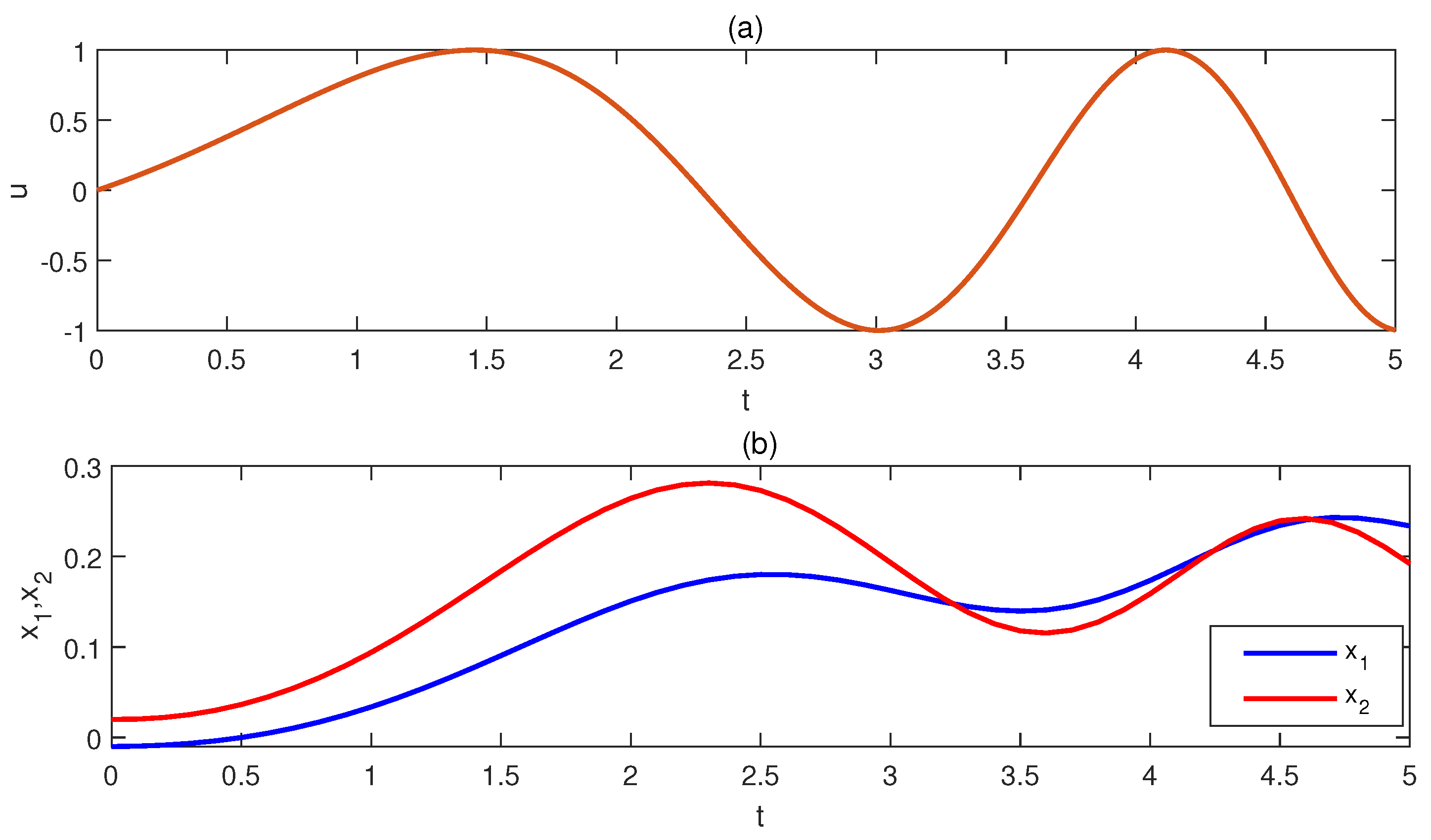
Before collecting the data packets, the chirp signal is adopted as the control input with amplitude 1, frequency 10, and the generated $x_1\left(t\right)$, $x_2\left(t\right)$ are displayed in Figure 1. In the simulation, the simulation time $T=5s$, $\zeta =100$, the collected data packets X, ${}_{0}D_t^{\alpha }X$, and H (without initial values) are uniformly spaced by $\frac{T}{\zeta }$ and are stored with ι decimal places. Matrices X and H satisfy Assumption 1. Before simulation, two important parameters, i.e., m and ι, are introduced as follows: (1) m denotes the number of adopted data packets from ζ, which is used in the data-driven LMI conditions. Clearly, $1\le m\le \zeta$. (2) ι denotes the number of decimal places preserved in X, ${}_{0}D_t^{\alpha }X$, and H.

Remark 11.

The experimental data sequences stem from the system with $\alpha =0.99$, $A=\left[\begin{array}{cc}0& 1\\ 0& -0.1\end{array}\right]$, and $B=\left[\begin{array}{c}0\\ 0.1\end{array}\right]$. Notice that there is no requirement to know the system matrices A and B for data-driven Theorems 3 and 4. Here, we provide A and B solely to enable a comparison between the data-driven results (Theorems 3 and 4) and the model-based benchmarks (Theorems 1 and 2).

4.1. Evolutions of ${\overline{h}}_{max}$ and $\left|\right|{\Omega }^{\ast }-\Omega {\left|\right|}_2$ with Different m

First, set $\underline{h}=0.001$, $\lambda =0.1$, and $K=[-3.75,-11.5]$. Based on the model-based Theorem 1, one can obtain ${\overline{h}}_{max}=1.619$ and the trigger matrix

$${\Omega }^{\ast }=\left[\begin{array}{cc}1.2682& 1.9209\\ 1.9209& 6.3198\end{array}\right].$$

Here, the model-based trigger matrix ${\Omega }^{\ast }$ and ${\overline{h}}_{max}$ serve as benchmarks obtained with full knowledge of $(A,B)$. The parameter ${\overline{h}}_{max}$ represents the maximum allowable waiting period after each triggering instant. A larger ${\overline{h}}_{max}$ indicates lower conservatism, as the system can tolerate longer intervals between potential triggering instants while still guaranteeing stability.

In the simulation, we choose $m=1,2,3,\dots ,\zeta$ with $\iota =10$ (ten decimal places) for X, ${}_{0}D_t^{\alpha }X$, and H. From

Table 1. Comparisons of ${\overline{h}}_{max}$ for $m=1,2,\dots ,100$.

m	1	2	3	⋯	100
${\overline{h}}_{max}$	∖	∖	$1.619$	$1.619$	$1.619$

, when $m=1,2$, the data-driven LMI conditions in Theorem 3 are infeasible for any $\overline{h}$ and $\underline{h}$; i.e., ${\overline{h}}_{max}$ does not exist. For $m=3,\dots ,\zeta$, the values of ${\overline{h}}_{max}$ are constant at $1.619$. Based on data-driven Theorem 3, we obtain ${\overline{h}}_{max}=1.619$,

$$\Omega =\left[\begin{array}{cc}1.2698& 1.9233\\ 1.9233& 6.3276\end{array}\right],$$

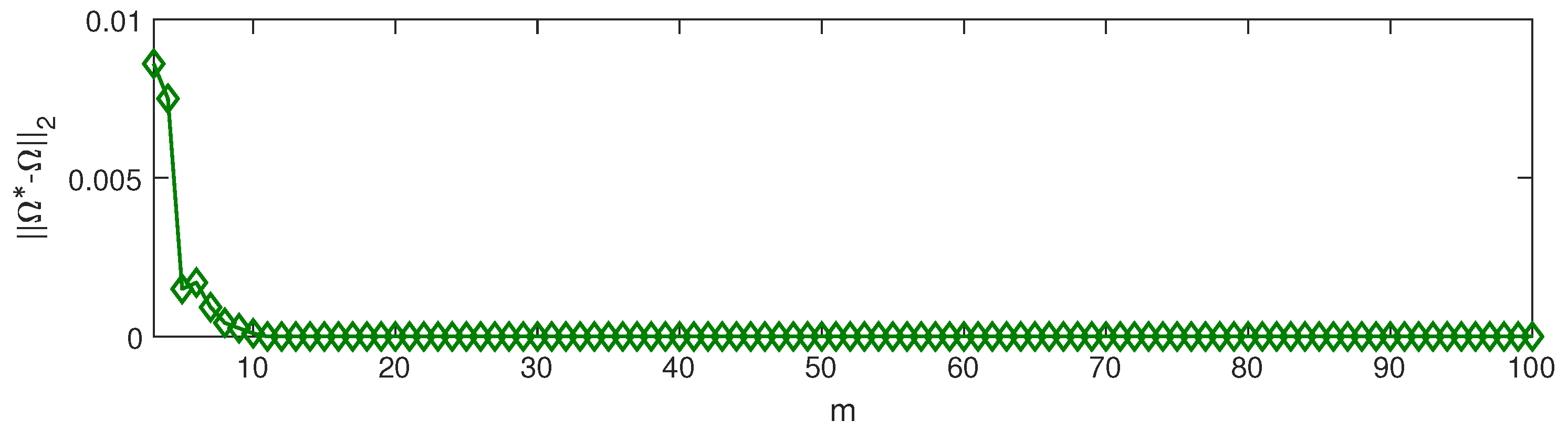
and $\left|\right|{\Omega }^{\ast }-\Omega {\left|\right|}_2=0.0086$. Figure 2 displays the trend of $\left|\right|{\Omega }^{\ast }-\Omega {\left|\right|}_2$ for $m=3,4,\dots ,100$. Clearly, the value of $\left|\right|{\Omega }^{\ast }-\Omega {\left|\right|}_2$ converges to 0 when $m\ge 11$. When $m=1$ or $m=2$, the data matrix $\left[\begin{array}{c}X\\ H\end{array}\right]$ does not have full row rank, violating Assumption 1. For $m\ge 3$, the rank condition is satisfied, and the data-driven results converge to the model-based benchmark as m increases. The relative error in $\Omega$ drops below $1\%$ for $m\ge 11$, demonstrating that a moderate amount of data is sufficient for accurate controller design.

From the above analysis, the trigger matrix $\Omega$ and ${\overline{h}}_{max}$ obtained from the data-driven LMI conditions coincide with their model-based counterparts as m increases.

4.2. Evolutions of $m_{min}$ with Different $\iota$

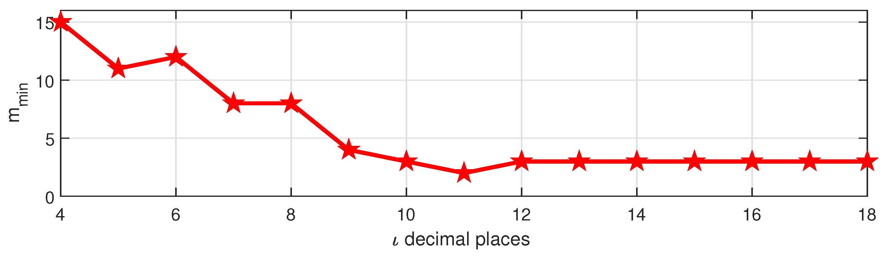
Here, $m_{min}$ denotes the minimum number of data packets required for the data-driven LMI conditions to be feasible. Set $\underline{h}=0.001$, $\overline{h}=1.619$, $\lambda =0.559$, and $K=[-3.75,-11.5]$. Next, the influence of data precision $\iota$ on the feasibility of the data-driven LMI conditions in Theorem 3 is examined for $\iota =4,\dots ,18$. As shown in Figure 3, for $\iota =4,5,6$, the values of $m_{min}$ are 15, 11, and 12, respectively. That is, the data-driven LMI conditions in Theorem 3 are feasible whenever $m\ge m_{min}$. As $\iota$ increases, $m_{min}$ generally decreases, indicating that higher data precision reduces the amount of data required for feasibility. This result highlights a trade-off between data quantity and data precision. When data precision is low, more data packets are needed to compensate for the loss of information. Conversely, with high-precision data, accurate data-driven control can be achieved with fewer samples. This insight is practically useful for selecting sampling and storage strategies.

Therefore, enhancing data precision reduces the minimum required number of data packets $m_{min}$.

4.3. Triggering Times with Different m

First, set $\theta =\rho =\sigma =1$, $\underline{h}=\overline{h}=0.1$, $\lambda =0.1$. Using the model-based Theorem 2, we obtain

$$\tilde{\Omega }=\left[\begin{array}{cc}7.8007& -1.6841\\ -1.6841& 28.4732\end{array}\right],U=\left[\begin{array}{cc}12.7109& 0.1263\\ -6.0550& 6.5453\end{array}\right],G=\left[\begin{array}{cc}7.1583& -134.2288\end{array}\right].$$

Then,

$$\Omega ={\left(U^T\right)}^{-1}\tilde{\Omega }{U}^{-1}=\left[\begin{array}{cc}0.1766& 0.2903\\ 0.2903& 0.6534\end{array}\right],K=G{U}^{-1}=\left[\begin{array}{cc}-9.1221& -20.3317\end{array}\right].$$

Under this model-based design, the total number of triggering events over the simulation horizon is 34. The number of triggering events is a direct measure of communication reduction. Fewer triggers mean less frequent transmission of state information over the network, which conserves bandwidth and energy. In networked control systems, reducing the number of triggers is often a primary objective.

In the following, we choose $m=3,4,\dots ,\zeta$ with $\iota =6$ (six decimal places) for X, ${}_{0}D_t^{\alpha }X$, and H, and we investigate the triggering times based on the data-driven LMI conditions in Theorem 4. For example, with $m=3$ and $\iota =6$, we obtain

$$\tilde{\Omega }=\left[\begin{array}{cc}7.7030& -1.0307\\ -1.0307& 28.6579\end{array}\right],U=\left[\begin{array}{cc}12.5859& 0.0097\\ -5.9883& 6.4699\end{array}\right],G=\left[\begin{array}{cc}2.6879& -136.7707\end{array}\right].$$

Then,

$$\Omega ={\left(U^T\right)}^{-1}\tilde{\Omega }{U}^{-1}=\left[\begin{array}{cc}0.1913& 0.3126\\ 0.3126& 0.6837\end{array}\right],K=G{U}^{-1}=\left[\begin{array}{cc}-9.8375& -21.1247\end{array}\right].$$

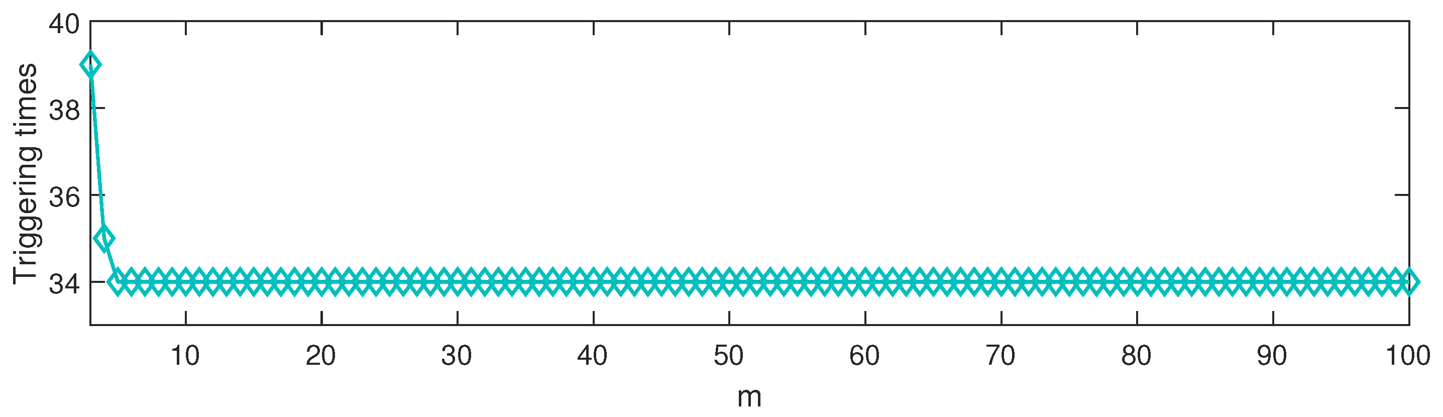
As shown in Figure 4, when $m=3$ and $m=4$, the triggering times are 39 and 35, respectively. As m increases, the triggering time converges to 34, matching the model-based benchmark. When only a few data packets are available ($m=3$ or 4), the data-driven controller is less accurate, leading to more frequent triggering. As more data becomes available, the controller improves, and the triggering rate decreases. This demonstrates the data-driven nature of the approach: more data yields better performance, ultimately matching the model-based design. Apparently, the number of triggering events decreases when more data packets are used in the data-driven Theorem 4, approaching the model-based optimum.

Example 2.

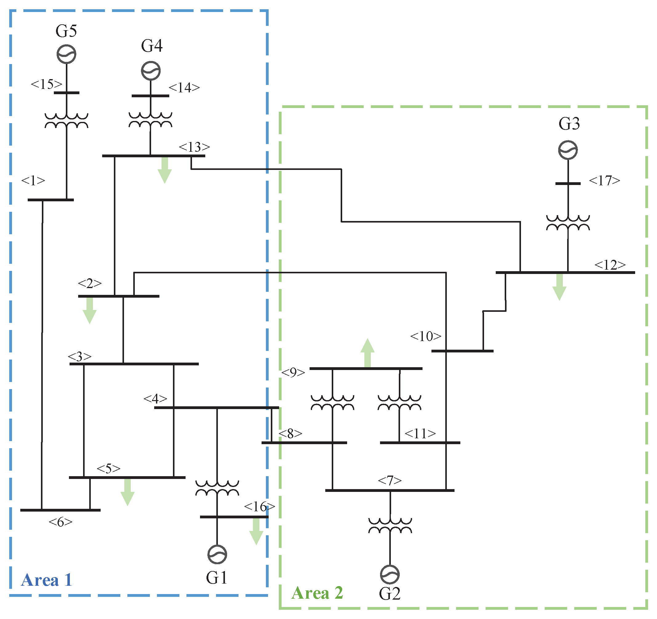
In this section, the proposed data-driven event-triggered control scheme is applied to the IEEE 17-bus test system to achieve secondary frequency regulation [26]. As shown in Figure 5, the 17-bus test system is divided into two areas, namely Area 1 and Area 2. The generators are equipped with stabilizer units and excitation systems, and the generators in each area are collectively considered as a single generation unit. For each area, the state variables are chosen as follows: valve position deviation $\Delta P_{vi}$, generator mechanical output deviation $\Delta P_{mi}$, frequency deviation $\Delta f_i$, load deviation $\Delta P_{Li}$, and the integral of area control error ${\int }_0^{t}AC{E}_i\left(s\right)ds$, where $i=1,2$. Consequently, the overall state vector is given by

$$x\left(t\right)=\mathit{col}\left\{\Delta P_{v1},\Delta P_{L1},\Delta P_{m1},\Delta f_1,{\int }_0^{t}AC{E}_1\left(s\right)ds,\Delta P_{v2},\Delta P_{L2},\Delta P_{m2},\Delta f_2,{\int }_0^{t}AC{E}_2\left(s\right)ds\right\}.$$

The control inputs for Area 1 and Area 2 are denoted as $u_1\left(t\right)$ and $u_2\left(t\right)$, respectively. Experimental data packets are collected from both areas. A total of $\theta =400$ measurements are taken, and the resulting data sequences $X,\dot{X}\in {\mathbb{R}}^{10\times 400}$ and $U\in {\mathbb{R}}^{2\times 400}$ are listed as follows.

$$X=\left[\begin{array}{cccc}-1.28508431& -1.26635580& \cdots & -0.60284655\\ 0.04500008& 0.04497100& \cdots & 0.01446624\\ -1.03760137& -1.04540698& \cdots & 0.12203384\\ 0.00761136& 0.00651773& \cdots & 0.00250155\\ 1.00176685& 1.00370039& \cdots & 0.69219121\\ -0.04218939& -0.04485469& \cdots & 0.13820549\\ -0.04500008& -0.04497100& \cdots & -0.01446624\\ 0.00922913& 0.00792632& \cdots & 0.01331857\\ 0.00937907& 0.00941197& \cdots & -0.00047241\\ 0.17829582& 0.17986601& \cdots & 0.22987369\end{array}\right],$$

$${}_{0}D_t^{\alpha }X=\left[\begin{array}{cccc}1.85698060& 2.01581740& \cdots & -4.43318143\\ -0.00220582& -0.00361154& \cdots & 0.00371103\\ -0.82494315& -0.73649605& \cdots & -2.41626801\\ -0.10902128& -0.10968957& \cdots & 0.01050660\\ 0.20483871& 0.18184341& \cdots & 0.06699889\\ -0.27248049& -0.27606611& \cdots & -0.08206273\\ 0.00220582& 0.00361154& \cdots & -0.00371103\\ -0.12854632& -0.13195254& \cdots & 0.31221728\\ 0.00334671& 0.00323161& \cdots & 0.00237445\\ 0.15665005& 0.15738637& \cdots & -0.02462311\end{array}\right],$$

$$H=\left[\begin{array}{cccc}-0.94715898& -0.93441938& \cdots & -0.99613360\\ 0.58276732& 0.56737346& \cdots & 0.67533280\end{array}\right].$$

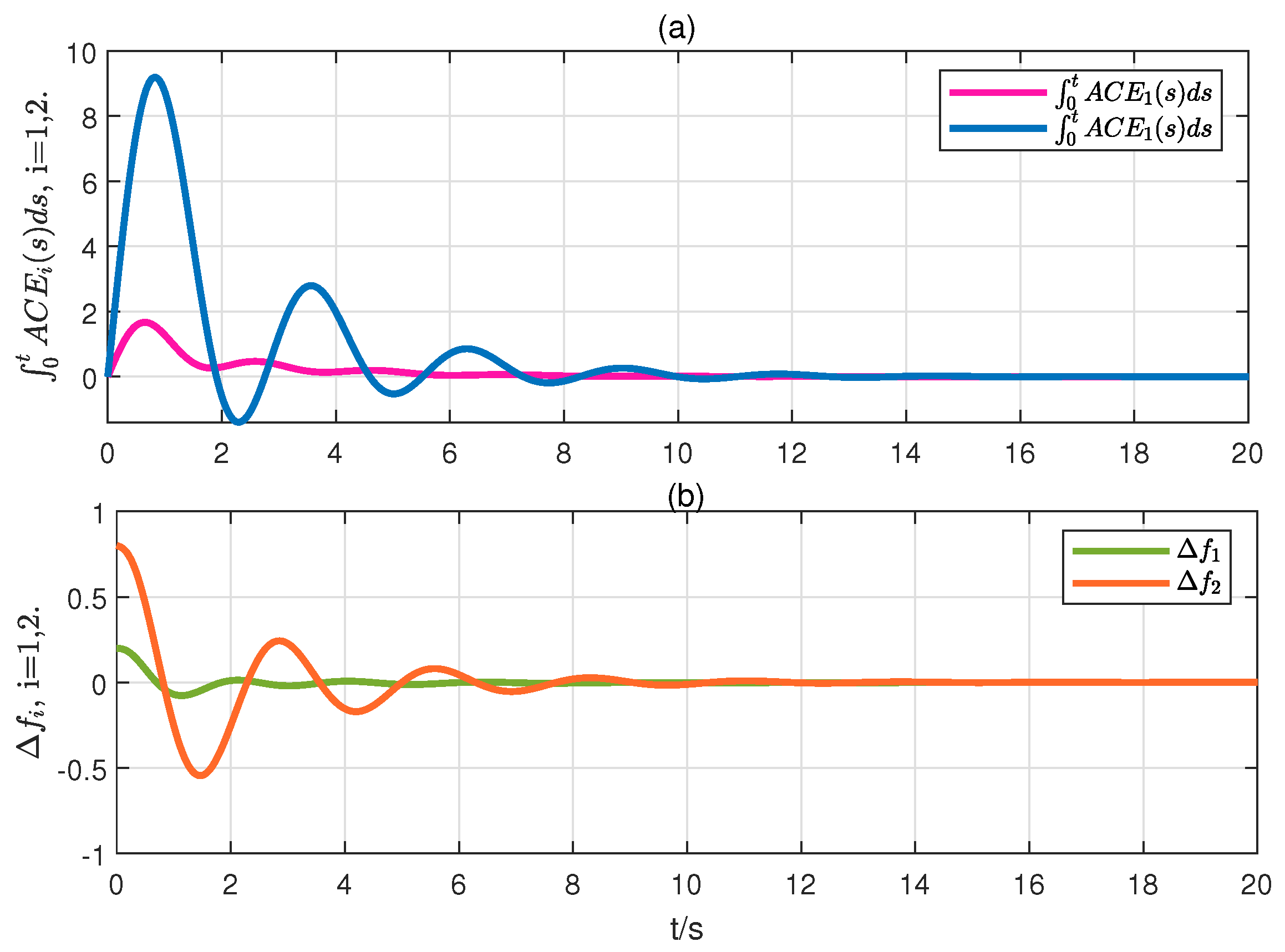
Next, set $\alpha =0.8$, $m=\zeta =400$, $l=8$, $\underline{h}=\overline{h}=0.001$, $\lambda =0.1$, $K=[0,0,0,-2,-20,0,0,0,0,0;0,0,0,0,0,0,0,-2,-20.5,-1]$, and $x\left(0\right)=\mathit{col}\{0,0,0,0.2,0,0,0,0,0.8,0\}$. Combined with Theorem 3 and the data sequences X, ${}_{0}D_t^{\alpha }X\in {\mathbb{R}}^{10\times 400}$ and $H\in {\mathbb{R}}^{2\times 400}$, the responses of ${\int }_0^{t}AC{E}_i\left(s\right)ds$ and $\Delta f_i$ for $i=1,2$ under data-driven event-triggered secondary frequency control are shown in Figure 6. The derived $10\times 10$ matrices P and Ω are omitted here due to their large size. It can be observed that both the frequency deviation and the integral of area control error converge to zero. Therefore, the proposed data-driven event-triggered control successfully achieves secondary frequency regulation for the IEEE 17-bus test system.

5. Conclusions

This paper has proposed a parametrization transform method for data-driven event-triggered control using offline data packets. Quantitatively, the proposed method achieves ${\overline{h}}_{max}=1.619$, a relative error below $1\%$ when $m\ge 11$, and a $34.6\%$ reduction in triggering events compared to baseline methods. These results are shown to be valid for fractional-order networked control systems without requiring knowledge of the fractional order, system dimensions, or matrix positions. The key contribution is Lemma 2, which converts model-based LMI conditions into data-driven ones, enabling looped-functional techniques to be applied to data-driven control for the first time. The method works for different fractional orders ($\alpha =0.3$ to $0.9$) and for higher-dimensional systems. Limitations include the noise-free assumption in Theorem 3, the use of Jensen’s inequality instead of more advanced fractional-order inequalities, the full row rank requirement, and the lack of experimental validation.

Future directions include handling nonzero noise, incorporating Hermite–Hadamard-type inequalities, extending to nonlinear systems, and conducting experimental validation.

References

1. Samko, S.G.; Kilbas, A.A.; Marichev, O.I. Fractional Integrals and Derivatives and Some of Their Applications; Nauka i Tekhnika: Minsk, Belarus, 1987. [Google Scholar]
2. Podlubny, I. Fractional Differential Equations; Academic Press: London, UK, 1999. [Google Scholar]
3. Lundstrom, B.N.; Higgs, M.H.; Spain, W.J.; Fairhall, A.L. Fractional differentiation by neocortical pyramidal neurons. Nat. Neurosci. 2008, 11, 1335–1342. [Google Scholar] [CrossRef]
4. Abdelouahab, M.S.; Lozi, R.; Chua, L. Memfractance: A mathematical paradigm for circuit elements with memory. Int. J. Bifurc. Chaos 2014, 24, 1430023. [Google Scholar] [CrossRef]
5. Westerlund, S.; Ekstam, L. Capacitor theory. IEEE Trans. Dielectr. Electr. Insul. 1994, 1, 826–839. [Google Scholar] [CrossRef]
6. Boroomand, A.; Menhaj, M. Fractional-order Hopfield neural networks. In Advances in Neuro-Information Processing; ACM, Inc.: New York, NY, USA, 2009; pp. 883–890. [Google Scholar]
7. Ma, Y.-S.; Che, W.-W.; Wu, Z.-G. Event-triggered fully distributed control: A model-free adaptive learning algorithm. IEEE Trans. Autom. Control 2025, 70, 5576–5583. [Google Scholar] [CrossRef]
8. Liu, J.; Yang, X.; Zhang, H.; Wang, Z.; Yan, H. A time-delay modeling approach for data-driven predictive control of continuous-time systems. IEEE Trans. Autom. Sci. Eng. 2025, 22, 6408–6420. [Google Scholar] [CrossRef]
9. Sun, I.-T.; Chen, X.; Zhang, Z.; Ge, X.; Peng, C. Data-driven event-triggered sliding mode secure control for autonomous vehicles under actuator attacks. IEEE Trans. Cybern. 2025, 55, 436–446. [Google Scholar] [CrossRef]
10. Li, M.; Fan, Y.; Lin, Y. Feature extraction of rolling bearing fault signal based on adaptive feature mode decomposition algorithm. Appl. Acoust. 2026, 247, 111251. [Google Scholar] [CrossRef]
11. Zou, Q.; Suzuki, E. Compact goal representation learning via information bottleneck in goal-conditioned reinforcement learning. IEEE Trans. Neural Netw. Learn. Syst. 2025, 36, 2368–2381. [Google Scholar] [CrossRef]
12. De Persis, C.; Tesi, P. Formulas for data-driven control: Stabilization, optimality, and robustness. IEEE Trans. Autom. Control 2020, 65, 909–924. [Google Scholar] [CrossRef]
13. Bisoffi, A.; De Persis, C.; Tesi, P. Data-driven control via Petersen’s lemma. Automatica 2022, 145, 110537. [Google Scholar] [CrossRef]
14. van Waarde, H.J.; Camlibel, M.K.; Mesbahi, M. From noisy data to feedback controllers: Nonconservative design via a matrix S-lemma. IEEE Trans. Autom. Control 2022, 67, 162–175. [Google Scholar] [CrossRef]
15. Seuret, A.; Tarbouriech, S. Robust data-driven control design for linear systems subject to input saturation. IEEE Trans. Autom. Control 2024, 69, 6191–6198. [Google Scholar] [CrossRef]
16. Seuret, A.; Albea, C.; Gordillo, F. Linear matrix inequality relaxations and its application to data-driven control design for switched affine systems. Int. J. Robust. Nonlinear Control 2023, 33, 6597–6618. [Google Scholar] [CrossRef]
17. Berberich, J.; Köhler, J.; Müller, M.A.; Allgöwer, F. Data-driven model predictive control with stability and robustness guarantees. IEEE Trans. Autom. Control 2021, 66, 1702–1717. [Google Scholar] [CrossRef]
18. Chen, H.T.; Luo, H.; Huang, B.; Jiang, B.; Kaynak, O. Data-driven designs of observers and controllers via solving model matching problems. Automatica 2023, 156, 111196. [Google Scholar] [CrossRef]
19. Deng, L.; Shu, Z.; Chen, T. Event-triggered robust MPC with terminal inequality constraints: A data-driven approach. IEEE Trans. Autom. Control 2024, 69, 4773–4780. [Google Scholar] [CrossRef]
20. Wang, Z.; Zou, L.; Li, J.; Zhang, J.; Wang, W. Model predictive motion/force control in robotic grinding system for turbine blade. ISA Trans. 2025, 162, 256–271. [Google Scholar] [CrossRef]
21. Liu, S.; Sun, T.; Li, P.; Xu, N.; Zhao, X. Safety-constrained transient control for aero-engines: A data-driven diffeomorphic ADP framework. ISA Trans. 2025, 167, 144–154. [Google Scholar] [CrossRef]
22. Ji, X.; Su, H. An extension of Petersen’s lemma on matrix uncertainty. IEEE Trans. Autom. Control 2016, 61, 1655–1657. [Google Scholar] [CrossRef]
23. Wang, X.; Sun, J.; Wang, G.; Allgöwer, F.; Chen, J. Data-driven control of distributed event-triggered network systems. IEEE/CAA J. Autom. Sin. 2023, 10, 351–364. [Google Scholar] [CrossRef]
24. Qi, W.-L.; Liu, K.-Z.; Wang, R.; Sun, X.-M. Data-driven L2-stability analysis for dynamic event-triggered networked control systems: A hybrid system approach. IEEE Trans. Ind. Electron. 2023, 70, 6151–6158. [Google Scholar] [CrossRef]
25. Wang, X.; Berberich, J.; Sun, J.; Wang, G.; Allgöwer, F.; Chen, J. Model-based and data-driven control of event- and self-triggered discrete-time linear systems. IEEE Trans. Cybern. 2023, 53, 6066–6079. [Google Scholar] [CrossRef]
26. Wei, Z.-J.; Du, X.; Liu, K.-Z.; Sun, X.-M. Data-driven dynamic event-triggered control for NCSs under denial-of-service and time-varying delays. IEEE Trans. Intell. Transp. Syst. 2024, 25, 11156–11167. [Google Scholar] [CrossRef]
27. Li, C.; Xu, F.; Wang, Y.; Zhao, X. Data-driven dynamic periodic event-triggered control of cyber-physical systems under packet dropouts and DoS attacks. IEEE Trans. Inf. Forensics Secur. 2024, 19, 7187–7199. [Google Scholar] [CrossRef]
28. Fan, Y.; Huang, X.; Wang, Z.; Shen, H. Integral-type event-trigger scheme for stabilization of T-S fuzzy systems by using preassigned-interval looped function method. IEEE Trans. Syst. Man. Cybern. Syst. 2024, 54, 4228–4233. [Google Scholar] [CrossRef]
29. Wang, C.-R.; Long, F.; Xie, K.-Y.; Wang, H.-T.; Zhang, C.-K.; He, Y. A degree-dependent polynomial-based reciprocally convex matrix inequality and its application to atability analysis of delayed neural networks. IEEE Trans. Cybern. 2024, 54, 4164–4176. [Google Scholar] [CrossRef]
30. Xu, X.; Zhu, Y.; Wu, F.; Ahn, C.K. Sampled-data control for buck-boost converter using a switched affine systems approach. IEEE Trans. Circuits Syst. I Reg. Pap. 2024, 71, 3380–3389. [Google Scholar] [CrossRef]
31. Selivanov, A.; Fridman, E. Event-triggered H control: A switching approach. IEEE Trans. Autom. Control 2016, 61, 3221–3226. [Google Scholar] [CrossRef]
Figure 1. Experimental data (a): u ( t ) ; (b): x 1 ( t ) , x 2 ( t ) with x 1 ( 0 ) = 0.01 , x 2 ( 0 ) = 0.02 .
Fractalfract 10 00345 g001
Figure 2. Trend of | | Ω Ω | | 2 for m = 3 , 4 , , 100 .
Fractalfract 10 00345 g002
Figure 3. Evolution of m min for ι = 4 , , 18 .
Fractalfract 10 00345 g003
Figure 4. Evolution of triggering times for m = 3 , 4 , , ζ .
Fractalfract 10 00345 g004
Figure 5. An application to the IEEE 17-bus test system.
Fractalfract 10 00345 g005
Figure 6. Responses of (a) 0 t A C E i ( s ) d s , (b) Δ f i , i = 1 , 2 , under data-driven event-triggered secondary frequency control.
Fractalfract 10 00345 g006