Straightforward Design of a Robust Fractional-Order Controller

Abstract

Fractional-order controllers have emerged as robust alternatives to conventional PID controllers. Existing tuning methods generally focus solely on robustness to process gain variations. This paper introduces a design method for fractional-order PI controllers, specifically resilient to time constant changes by shaping the loop frequency response. This work simplifies the design method by replacing the separate magnitude and phase derivative calculations used in prior techniques with a unified, single partial derivative approach. Instead of using cumbersome optimization routines and graphical analysis used in existing fractional-order controller tuning methods, the proposed approach uses a direct, simple, and efficient 1-step algorithm. Numerical simulations for lag- and delay-dominant processes are included to highlight the efficiency of the proposed approach. Traditional integer order controllers are designed for comparative purposes. The proposed approach achieves a constant overshoot despite time constant variations, an advantage compared to classical controllers.

1. Introduction

The fractional-order PID (FO-PID) generalizes classical PID control [1], offering superior flexibility, reduced control effort, and enhanced performance for time-delay systems [2]. They have recently been used in sophisticated control structures [3,4], a premise towards further enhancing research in the area of tuning more and more performant FO-PIDs. This motivates the use of these controllers in this research, as well. Most tuning methods utilize the frequency domain due to its mathematical simplicity compared to the time domain, indirectly targeting criteria such as settling time, overshoot, steady-state accuracy, and disturbance rejection [1,2]. Other, more advanced tuning methods include metaheuristic optimization algorithms, hybrid approaches involving reinforcement learning, data-driven approaches, or auto-tuning [5,6,7,8], to name just a few.

A primary benefit of FO-PID controllers is the increased closed-loop robustness they provide [9,10] relative to classical PID architectures. Several review papers [1,11,12] provide extensive surveys on fractional-order PID design for various processes, including discussions on their inherent robustness. Extensive research [13,14,15,16,17,18,19] has focused on ensuring robustness specifically against plant gain variations, across diverse systems, from simple first-order plants to complex processes with significant dead time. Researchers have moved beyond standard metrics, employing a combination of phase margin, gain margin, and iso-damping specifications [13]. For example, Ref. [14] integrates frequency-domain constraints with the Integral Time Absolute Error (ITAE) to enhance resilience, while [18] utilizes the Integral of Absolute Error (IAE) alongside a maximum sensitivity constraint.

Alternative strategies incorporate Bode’s ideal loop transfer function, often featuring additional delay terms or filters [15,17], though these primarily evaluate robustness against gain fluctuations. The iso-damping property—essential for maintaining a constant overshoot despite gain changes—remains a focal point in methods derived from Bode’s ideal loop [19]. Internal Model Control (IMC) approaches [20] have been used to meet specific gain crossover frequency and phase margin targets, with experimental validation on DC motor setups.

Few research papers deal with robustness to other process parameters. The tuning procedure is, however, tedious and not straightforward. Probabilistic robustness [21] or multi-objective genetic algorithms [22] are used to handle parameter uncertainties, though these often lack direct tuning rules. The parameters of the FO-PIDs are often estimated using optimization routines that involve the minimization of indices such as Integral of Absolute Error (IAE), overshoot, and settling time. These optimization routines usually depend on the choice of the initial conditions, the maximum number of iterations, global convergence, and computational efficiency. These factors make the computation of the FO-PID parameters a non-trivial task that demands significant expertise in optimization routines. While [23] considers robustness to both gain and time constant variations using phase and gain margin specifications, it lacks a systematic tuning procedure for time constant resilience. Alternative strategies employ cascaded FO-PI structures optimized for IAE [24]. A tuning methodology for fractional-order controllers using interval pole placement is introduced in [25]. Validated on a thermal plant, this approach improves transient response and control effort while offering superior robustness compared to traditional robust control techniques. In [26], the authors developed an FO-PID design method that targets specific phase margins, gain crossover frequencies, and iso-damping properties. This approach specifically addresses variations in the undamped natural frequency for oscillatory systems, though it is limited to minimum phase rational transfer functions where pole-zero combinations satisfy the interlacing property on the imaginary axis.

Robust stabilization for uncertainties across all parameters is tackled in [27,28,29,30,31]. While D-K iterations are used in [27] for interval plants, no explicit tuning rules are indicated in [28]. CRONE controllers [29] have been applied to wind energy systems [30], but all these procedures remain notoriously tedious. Other approaches [31] define a stability area for FO-PID parameters in uncertain FOPDT processes, but, like many existing studies, they stop short of offering an exact, step-by-step parameter determination procedure.

While most research focuses on tuning FO-PID controllers for robustness to gain variations, recent studies have introduced practical design methods that also address time constant variations. In [32], a fractional-order [PD] controller tuning algorithm that incorporates a third constraint to ensure robustness against time constant variations, based on gain crossover and phase margin criteria, is introduced. The core strategy involves analyzing the gradient of the phase margin and crossover frequency to changes in both the process time constant and the operating frequency. Due to the nonlinear nature of the resulting equations, optimization algorithms are employed to find a solution. Additionally, the paper provides specific parameter constraints and criteria for selecting the optimal gain crossover frequency. Using optimization to solve resulting nonlinear equations, the method is validated through simulation and experimental results demonstrating efficiency across ±20% variations. An updated iso-damping method using min-max optimization is presented in [33]. When applied to a Fractional-Order Plus Delay Time (FOPDT) process, this approach maintains performance even with parameter fluctuations of up to 30%. A similar idea to [32] is reiterated in [34] to demonstrate the practical range of phase margins and gain crossover frequencies that ensure robustness against time constant variations. By defining these operational limits, the authors showcase the broad applicability of their tuning method. A more general approach presented in [9] focuses on FO-PID design for systems with one uncertain parameter. By calculating the partial derivatives of the phase margin and gain crossover frequency with respect to that parameter, the method ensures a stable phase margin. These sensitivity measures are then used as constraints within an optimization-based tuning process. These previous studies rely on partial derivatives to quantify and ensure robustness against time constant fluctuations. While these methods aim to satisfy specific gain crossover frequencies and phase margins by solving systems of nonlinear equations, they generally still require optimization routines to find a solution [9,32,33,34]. Recent studies have applied a similar methodology to biomedical and industrial systems [35,36], by extending the design methodology to different kinds of fractional-order controllers, such as FO-PIs and FO-PIDs. Experimental validation of these techniques is included in [32]. By utilizing the partial derivatives of the phase margin and crossover frequency with respect to plant parameters, these controllers maintain a consistent overshoot despite fluctuations in the time constant. Instead of using optimization routines to estimate the controller parameters, these new papers [35,36,37], use a graphical solution for the system of nonlinear equations. This makes the design more accessible for practical engineering without requiring exhaustive optimization.

This paper builds on the partial derivative-based robustness techniques found in [9,32,33,34,35,36,37], while incorporating specific requirements for phase margin and gain crossover frequency. Unlike previous methods that separately calculate derivatives for both the magnitude and phase of the loop response, this work proposes a more elegant, unified approach using a single partial derivative of the loop frequency response. Furthermore, the tuning process for FO-PI parameters is streamlined by replacing optimization routines and graphical methods with a straightforward, simple 1-step procedure without iterations.

The original elements of the paper consist in: a novel design approach for FO-PIs; a simplification of existing FO-PI tuning methods for robustness to time constant variations; FO-PIs that are robust to time constant variations, rather than gain variations (frequently encountered in research papers). The advantages of the proposed approach consist of a reduced mathematical overhead. The contribution of the research is three-fold: the development of the analytical equations for designing a FO-PI controller that is robust to time constant variations; the development of a simple 1-step approach to determine the parameters of the FO-PI controller; the implementation, testing, and comparative analysis of the proposed approach with a traditional PI controller for lag- and delay-dominant processes.

The use of a unified partial derivative reduces the analytical effort necessary to satisfy the robustness constraints found in [9,32,33,34,35,36,37]. Additionally, the proposed algorithm eliminates the need for specialized knowledge on optimization routines or graphical analysis. Without requiring any iterations, the proposed algorithm is a straightforward procedure that enables faster parameter tuning, making it more suitable for industrial applications compared to [9,21,22,32,33,34,35,36,37].

This paper is structured as follows. It presents a robust fractional-order controller, detailing its theoretical framework and design procedure in Section 2. It then demonstrates application through numerical examples of FOPDT processes in Section 3, followed by concluding remarks and future work in Section 4.

2. Design of a Robust Fractional-Order PI Controller

Consider a process described by a FOPDT model as indicated next:

$$P\left(s\right)={\displaystyle \frac{k}{Ts+1}}{e}^{-\tau s}$$

(1)

where k is the process gain, $\tau$ is the dead time, and T is the time constant. Using FOPDT models is standard practice in industrial process control [38]. The FOPDT model in Equation (1) is highly representative of a vast majority of industrial chemical, thermal, or biological systems. While real industrial systems are often higher order, the FOPDT models can be used as linear approximations that capture the essential dynamics, in terms of process gain, dead time, and dominant time constant. Additionally, working with a simplified FOPDT model enables an easier and faster design of the controllers.

The process is controlled via a fractional-order PI (FO-PI) controller, described as:

$$C\left(s\right)={k_p^{\lambda }{\left(1+{\displaystyle \frac{1}{T_{i}s}}\right)}^{\lambda }=\left(k_p+{\displaystyle \frac{k_i}{s}}\right)}^{\lambda }$$

(2)

where $\lambda \in \left(0, 1\right)$ is the fractional order, k_p and k_i are the proportional and integral gains, and T_i is the integral time constant. Denoting $C_1\left(s\right)=k_p+{\displaystyle \frac{k_i}{s}}$, it follows that the FO-PI controller in Equation (2) can be written in a more compact form, such as:

$$C\left(s\right)={C_1\left(s\right)}^{\lambda }$$

(3)

Considering a unit negative feedback system, the controller C(s) can also be defined as:

$$C\left(s\right)={\displaystyle \frac{L\left(s\right)}{P\left(s\right)}}$$

(4)

where L(s) is the open-loop transfer function. Using the previous notation $C_1\left(s\right)=k_p+{\displaystyle \frac{k_i}{s}}$, the proportional and integral gains are obtained as:

$$k_p=\mathfrak{R}e\left(C_1\left(j\omega \right)\right)$$

(5)

$$k_i=-\omega ·\mathcal{I}m\left(C_1\left(j\omega \right)\right)$$

(6)

and $T_i={\displaystyle \frac{k_p}{k_i}}$. The frequency response of L(s) is defined as:

$$L\left(j\omega \right)=M(\omega )·e^{j\phi \left(\omega \right)}=\left|L\left(j\omega \right)\right|·e^{j\angle L\left(j\omega \right)}$$

(7)

The loop frequency response (FR) in Equation (7) specifies the dynamics of the open-loop system at any frequency, $\omega$. The frequency response shows how a system behaves when a sinusoidal signal of a certain frequency and amplitude is applied at its input. The magnitude M = $\left|L\left(j\omega \right)\right|$ in Equation (7) shows the ratio of the output signal amplitude to the input signal amplitude. The phase $\phi =\angle L\left(j\omega \right)$ shows the shift of the output signal with respect to the input signal. The loop FR $L\left(j\omega \right)$ in Equation (7) can be mathematically expressed as a complex number.

To achieve the desired settling time and overshoot, the gain crossover frequency (${\omega }_c$) and phase margin (PM) are selected as design specifications. The loop frequency response is then calculated using Equation (7) as follows:

$$L\left(j{\omega }_c\right)=1·e^{j(-{180}^{\circ }+PM)}$$

(8)

The process frequency response at the gain crossover frequency is directly computed using Equation (1) as:

$$P\left(j{\omega }_c\right)={\displaystyle \frac{k}{j{\omega }_{c}T+1}}{e}^{-j{\omega }_c\tau }$$

(9)

By substituting Equations (8) and (9) into Equation (4), the controller frequency response is directly determined and then used to calculate the three tuning parameters: $k_p$, $k_i$, and $\lambda$.

Beyond the gain crossover frequency and phase margin, a third criterion ensures robustness to process time constant (T) variations. Since fluctuations in T directly impact both ${\omega }_c$ and PM, this requirement is critical for maintaining stability. For the system to be robust to changes in the time constant T, the following equations must hold [32]:

$${\left.{\displaystyle \frac{\mathsf{\partial }\left|L\left(j\omega \right)\right|}{\mathsf{\partial }\omega }}\right|}_{\left({\omega }_c,T_0\right)}\mathit{\Delta }\omega +{\left.{\displaystyle \frac{\mathsf{\partial }\left|L\left(j\omega \right)\right|}{\mathsf{\partial }T}}\right|}_{\left({\omega }_c,T_0\right)}\mathit{\Delta }T=0$$

(10)

$${\left.{\displaystyle \frac{\mathsf{\partial }\angle L\left(j\omega \right)}{\mathsf{\partial }\omega }}\right|}_{\left({\omega }_c,T_0\right)}\mathit{\Delta }\omega +{\left.{\displaystyle \frac{\mathsf{\partial }\angle L\left(j\omega \right)}{\mathsf{\partial }T}}\right|}_{\left({\omega }_c,T_0\right)}\mathit{\Delta }T=0$$

(11)

which can be rearranged to yield:

$${\displaystyle \frac{{\left.\frac{\mathsf{\partial }\left|L\left(j\omega \right)\right|}{\mathsf{\partial }\omega }\right|}_{\left({\omega }_c,T_0\right)}}{{\left.\frac{\mathsf{\partial }\left|L\left(j\omega \right)\right|}{\mathsf{\partial }T}\right|}_{\left({\omega }_c,T_0\right)}}}={\displaystyle \frac{{\left.\frac{\mathsf{\partial }\angle L\left(j\omega \right)}{\mathsf{\partial }\omega }\right|}_{\left({\omega }_c,T_0\right)}}{{\left.\frac{\mathsf{\partial }\angle L\left(j\omega \right)}{\mathsf{\partial }T}\right|}_{\left({\omega }_c,T_0\right)}}}$$

(12)

The robustness condition in Equation (12) has also been used in [9,32,33,34,35,36,37]. A detailed explanation of the link between the two equations in Equations (10) and (11) and the idea of maintaining a constant phase margin despite time constant variations is included in [32] and omitted for brevity in this paper.

The focus of this research falls on a novel approach that replaces Equations (10) and (11) with a single derivative, as indicated next. First, the result in Equation (11) is multiplied by ${j\left|L\left(j\omega \right)\right|}_{\left({\omega }_c,T_0\right)}$, yielding:

$$j{\left.{\displaystyle \frac{\mathsf{\partial }\angle L\left(j\omega \right)}{\mathsf{\partial }\omega }}\right|}_{\left({\omega }_c,T_0\right)}{\left|L\left(j\omega \right)\right|}_{\left({\omega }_c,T_0\right)}\mathsf{\Delta }\omega +j{\left.{\displaystyle \frac{\mathsf{\partial }\angle L\left(j\omega \right)}{\mathsf{\partial }T}}\right|}_{\left({\omega }_c,T_0\right)}{\left|L\left(j\omega \right)\right|}_{\left({\omega }_c,T_0\right)}\mathsf{\Delta }T=0$$

(13)

The summation of Equations (10) and (13) results in:

$${\left.{\displaystyle \frac{\mathsf{\partial }\left|L\left(j\omega \right)\right|}{\mathsf{\partial }\omega }}\right|}_{\left({\omega }_c,T_0\right)}\mathsf{\Delta }\omega +{\left.{\displaystyle \frac{\mathsf{\partial }\left|L\left(j\omega \right)\right|}{\mathsf{\partial }T}}\right|}_{\left({\omega }_c,T_0\right)}\mathsf{\Delta }T+{j\left.{\displaystyle \frac{\mathsf{\partial }\angle L\left(j\omega \right)}{\mathsf{\partial }\omega }}\right|}_{\left({\omega }_c,T_0\right)}{\left|L\left(j\omega \right)\right|}_{\left({\omega }_c,T_0\right)}\mathsf{\Delta }\omega +{\left.j{\displaystyle \frac{\mathsf{\partial }\angle L\left(j\omega \right)}{\mathsf{\partial }T}}\right|}_{\left({\omega }_c,T_0\right)}{\left|L\left(j\omega \right)\right|}_{\left({\omega }_c,T_0\right)}\mathsf{\Delta }T=0$$

(14)

Rearranging Equation (14) yields:

$$\left({\left.{\displaystyle \frac{\mathsf{\partial }\left|L\left(j\omega \right)\right|}{\mathsf{\partial }\omega }}\right|}_{\left({\omega }_c,T_0\right)}+{j\left.{\displaystyle \frac{\mathsf{\partial }\angle L\left(j\omega \right)}{\mathsf{\partial }\omega }}\right|}_{\left({\omega }_c,T_0\right)}{\left|L\left(j\omega \right)\right|}_{\left({\omega }_c,T_0\right)}\right)\mathsf{\Delta }\omega +\left({\left.{\displaystyle \frac{\mathsf{\partial }\left|L\left(j\omega \right)\right|}{\mathsf{\partial }T}}\right|}_{\left({\omega }_c,T_0\right)}{\left.+j{\displaystyle \frac{\mathsf{\partial }\angle L\left(j\omega \right)}{\mathsf{\partial }T}}\right|}_{\left({\omega }_c,T_0\right)}{\left|L\left(j\omega \right)\right|}_{\left({\omega }_c,T_0\right)}\right)\mathsf{\Delta }T=0$$

(15)

Multiplying Equation (15) by $e^{j\angle L\left(j\omega \right)}$ results in:

$$\left({\left.{\displaystyle \frac{\mathsf{\partial }\left|L\left(j\omega \right)\right|}{\mathsf{\partial }\omega }}\right|}_{\left({\omega }_c,T_0\right)}{e}^{j\angle L\left(j\omega \right)}+{j\left.e^{j\angle L\left(j\omega \right)}{\displaystyle \frac{\mathsf{\partial }\angle L\left(j\omega \right)}{\mathsf{\partial }\omega }}\right|}_{\left({\omega }_c,T_0\right)}{\left|L\left(j\omega \right)\right|}_{\left({\omega }_c,T_0\right)}\right)\mathsf{\Delta }\omega +\left(e^{j\angle L\left(j\omega \right)}{\left.{\displaystyle \frac{\mathsf{\partial }\left|L\left(j\omega \right)\right|}{\mathsf{\partial }T}}\right|}_{\left({\omega }_c,T_0\right)}{\left.+j{e}^{j\angle L\left(j\omega \right)}{\displaystyle \frac{\mathsf{\partial }\angle L\left(j\omega \right)}{\mathsf{\partial }T}}\right|}_{\left({\omega }_c,T_0\right)}{\left|L\left(j\omega \right)\right|}_{\left({\omega }_c,T_0\right)}\right)\mathsf{\Delta }T=0$$

(16)

which can be rewritten as:

$$\left({\left.{\displaystyle \frac{\mathsf{\partial }\left|L\left(j\omega \right)\right|}{\mathsf{\partial }\omega }}\right|}_{\left({\omega }_c,T_0\right)}{e}^{j\angle L\left(j\omega \right)}+{\left.{\displaystyle \frac{\mathsf{\partial }{e}^{j\angle L\left(j\omega \right)}}{\mathsf{\partial }\omega }}\right|}_{\left({\omega }_c,T_0\right)}{\left|L\left(j\omega \right)\right|}_{\left({\omega }_c,T_0\right)}\right)\mathsf{\Delta }\omega +\left(e^{j\angle L\left(j\omega \right)}{\left.{\displaystyle \frac{\mathsf{\partial }\left|L\left(j\omega \right)\right|}{\mathsf{\partial }T}}\right|}_{\left({\omega }_c,T_0\right)}{\left.+{\displaystyle \frac{\mathsf{\partial }{e}^{j\angle L\left(j\omega \right)}}{\mathsf{\partial }T}}\right|}_{\left({\omega }_c,T_0\right)}{\left|L\left(j\omega \right)\right|}_{\left({\omega }_c,T_0\right)}\right)\mathsf{\Delta }T=0$$

(17)

Using Equation (7), the result in Equation (17) can be mathematically condensed into:

$${\displaystyle \frac{\mathsf{\partial }L\left(j\omega \right)}{\mathsf{\partial }\omega }}\mathsf{\Delta }\omega +{\displaystyle \frac{\mathsf{\partial }L\left(j\omega \right)}{\mathsf{\partial }T}}\mathsf{\Delta }T=0$$

(18)

which leads to:

$${\displaystyle \frac{\frac{\mathsf{\partial }L\left(j\omega \right)}{\mathsf{\partial }\omega }}{\frac{\mathsf{\partial }L\left(j\omega \right)}{\mathsf{\partial }T}}}=-{\displaystyle \frac{\mathsf{\Delta }T}{\mathsf{\Delta }\omega }}$$

(19)

with ${\displaystyle \frac{\mathsf{\Delta }T}{\mathsf{\Delta }\omega }}$ a real number. Instead of using the partial derivatives of both the magnitude and the phase of the loop frequency response as in Equation (12), a unified approach was developed using the partial derivative of the loop frequency response only, as in Equation (19).

The loop frequency response can be written as:

$$L\left(j\omega \right)={\left[k_p\left(1+{\displaystyle \frac{1}{{J\omega T}_i}}\right)\right]}^{\lambda }{\displaystyle \frac{k{e}^{-j\omega \tau }}{1+j\omega T}}$$

(20)

Applying now the logarithmic operator to Equation (20) yields:

$$\log L\left(j\omega \right)=\lambda \left[\log k_p+\log \left(1+{j\omega T}_i\right)-\log \left({j\omega T}_i\right)\right]+\log k-j\omega \tau -\log \left(1+j\omega T\right)$$

(21)

Taking the derivative of Equation (21) with respect to the frequency $\omega$ gives:

$${\displaystyle \frac{\mathsf{\partial }\log L\left(j\omega \right)}{\mathsf{\partial }\omega }}=\lambda \left({\displaystyle \frac{{jT}_i}{1+{j\omega T}_i}}-{\displaystyle \frac{1}{\omega }}\right)-j\tau -{\displaystyle \frac{jT}{1+j\omega T}}$$

(22)

while the derivative of Equation (21) with respect to the time constant T gives:

$${\displaystyle \frac{\mathsf{\partial }\log L\left(j\omega \right)}{\mathsf{\partial }T}}=-{\displaystyle \frac{j\omega }{1+j\omega T}}$$

(23)

Taking now the ratio of Equations (22) and (23) yields:

$${\displaystyle \frac{\frac{\mathsf{\partial }\log L\left(j\omega \right)}{\mathsf{\partial }\omega }}{\frac{\mathsf{\partial }\log L\left(j\omega \right)}{\mathsf{\partial }T}}}=-\lambda {\displaystyle \frac{T_i}{\omega }}{\displaystyle \frac{1+j\omega T}{1+{j\omega T}_i}}+\lambda {\displaystyle \frac{1+j\omega T}{j{\omega }^2}}+{\displaystyle \frac{\tau }{\omega }}\left(1+j\omega T\right)+{\displaystyle \frac{T}{\omega }}$$

(24)

which leads to:

$${\displaystyle \frac{\frac{\mathsf{\partial }\log L\left(j\omega \right)}{\mathsf{\partial }\omega }}{\frac{\mathsf{\partial }\log L\left(j\omega \right)}{\mathsf{\partial }T}}}=-\lambda {\displaystyle \frac{T_i}{\omega }}{\displaystyle \frac{\left(1+j\omega T\right)\left(1-j\omega T_i\right)}{1+{\omega }^2{T}_i^2}}-\lambda j{\displaystyle \frac{1+j\omega T}{{\omega }^2}}+{\displaystyle \frac{\tau }{\omega }}\left(1+j\omega T\right)+{\displaystyle \frac{T}{\omega }}$$

(25)

with the real and imaginary parts obtained as:

$$\mathfrak{R}=-\lambda {\displaystyle \frac{T_i}{\omega }}{\displaystyle \frac{1+{\omega }^{2}T{T}_i}{1+{\omega }^2{T}_i^2}}+\lambda {\displaystyle \frac{T}{\omega }}+{\displaystyle \frac{\tau }{\omega }}+{\displaystyle \frac{T}{\omega }}$$

(26)

$$\mathfrak{I}=-\lambda T_i{\displaystyle \frac{\left(T-T_i\right)}{1+{\omega }^2{T}_i^2}}-{\displaystyle \frac{\lambda }{{\omega }^2}}+\tau T$$

(27)

The following equations also hold:

$${\displaystyle \frac{\mathsf{\partial }\log L\left(j\omega \right)}{\mathsf{\partial }\omega }}={\displaystyle \frac{\frac{\mathsf{\partial }L\left(j\omega \right)}{\mathsf{\partial }\omega }}{L}}$$

(28)

$${\displaystyle \frac{ \mathsf{\partial }\log L\left(j\omega \right)}{\mathsf{\partial }T}}={\displaystyle \frac{\frac{\mathsf{\partial }L\left(j\omega \right)}{\mathsf{\partial }T}}{L}}$$

(29)

Taking the ratio of Equations (28) and (29) leads to:

$${\displaystyle \frac{\frac{\mathsf{\partial }\log L\left(j\omega \right)}{\mathsf{\partial }\omega }}{\frac{\mathsf{\partial }\log L\left(j\omega \right)}{\mathsf{\partial }T}}}={\displaystyle \frac{\frac{\mathsf{\partial }L\left(j\omega \right)}{\mathsf{\partial }\omega }}{\frac{\mathsf{\partial }L\left(j\omega \right)}{\mathsf{\partial }T}}}$$

(30)

According to Equation (19), the imaginary part of ${\displaystyle \frac{\frac{\mathsf{\partial }L\left(j\omega \right)}{\mathsf{\partial }\omega }}{\frac{\mathsf{\partial }L\left(j\omega \right)}{\mathsf{\partial }T}}}=0$. Thus, the imaginary part in Equation (27) should be null, yielding:

$$-\lambda T_i{\displaystyle \frac{\left(T-T_i\right)}{1+{\omega }^2{T}_i^2}}-{\displaystyle \frac{\lambda }{{\omega }^2}}+\tau T=0$$

(31)

This last equation can be used to compute the fractional-order $\lambda$ as:

$$\lambda ={\displaystyle \frac{{\omega }^2\tau T\left(1+{\omega }^2{T}_i^2\right)}{\left(1+{\omega }^{2}T{T}_i\right)}}$$

(32)

The algorithm to compute the parameters of the FO-PI controller is as follows.

Step 1. Given a certain phase margin and gain crossover frequency, compute the loop frequency response $L\left(j{\omega }_c\right)$, according to Equation (8). This results in a single complex number.

Step 2. Compute the process FR-value $P\left(j{\omega }_c\right)$, using Equation (9). This results in a single complex number.

Step 3. Compute the controller FR-value $C\left(j{\omega }_c\right)={\displaystyle \frac{L\left(j{\omega }_c\right)}{P\left(j{\omega }_c\right)}}$. This results in a single complex number.

Step 4. For $\lambda$ = ${\lambda }_{min}:0.01:1$, with ${\lambda }_{min}={\displaystyle \frac{\left({180}^{\circ }-PM\right)-\angle P\left(j{\omega }_c\right)}{{90}^{\circ }}},$ compute ${C_1\left(j{\omega }_c\right)=C\left(j{\omega }_c\right)}^{1/\lambda }$, based on Equation (3); compute $k_p$ and $k_i$, using Equations (5) and (6), respectively. Compute ${\lambda }_{new}={\displaystyle \frac{{{\omega }_c}^2\tau T\left(1+{{\omega }_c}^2{T}_i^2\right)}{\left(1+{{\omega }_c}^{2}T{T}_i\right)}}$ according to Equation (32).

Step 5. Evaluate $e={\lambda }_{new}-\lambda$. The final solution is obtained where e = 0.

The simple 1-step procedure in the algorithm avoids convergence issues. As indicated in Step 4 and Step 5 of the algorithm, for each $\mathrm{\lambda }$ in the range ${\mathrm{\lambda }}_{\mathrm{m}\mathrm{i}\mathrm{n}}$ to 1, the expression ${\mathrm{\lambda }}_{\mathrm{n}\mathrm{e}\mathrm{w}}-\mathrm{\lambda }$ is evaluated. The final solution for $\mathrm{\lambda }$, which fulfills the robustness condition, is obtained where ${\mathrm{\lambda }}_{\mathrm{n}\mathrm{e}\mathrm{w}}-\mathrm{\lambda }=0$. Finding a solution is not always guaranteed. For some choices of PM and/or ${\mathrm{\omega }}_{\mathrm{c}}$, there might be no solution. This is not the result of the proposed algorithm. Any other method would also fail because there simply does not exist a $\mathrm{\lambda }$-value that fulfills the robustness condition.

3. Numerical Simulation Results

The proposed method is validated using three numerical examples: a lag-dominant process (with a ratio ${\displaystyle \frac{T}{\tau }}=30$), a process with a ratio ${\displaystyle \frac{T}{\tau }}=2$, and a and a delay-dominant process (with a ratio ${\displaystyle \frac{T}{\tau }}=0.55$).

3.1. Example No. 1

A lag-dominant process with k = 1, $\tau =0.2$, and T = 6 is described by the following transfer function:

$$P_1\left(s\right)={\displaystyle \frac{1}{6s+1}}{e}^{-0.2s}$$

(33)

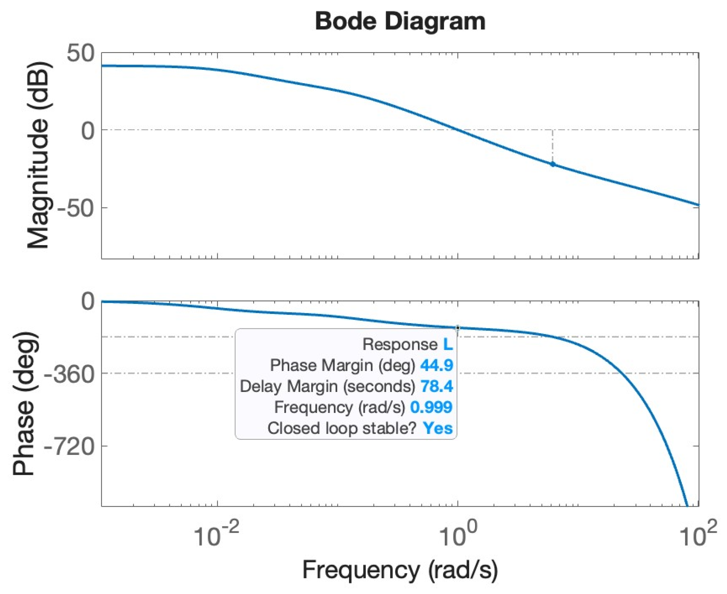
To tune the FO-PI controller, the following performance specifications are used: PM = 45°,${\omega }_c=1$ rad/s, and robustness to time constant variations. The algorithm presented in Section 2 yields the results indicated in

Table 1. Results obtained for process P₁(s).

Step 1	$L\left(j{\omega }_c\right)=-0.7071-j0.7071$
Step 2	$P\left(j{\omega }_c\right)=-0.0057-0.1643j$
Step 3	$C\left(j{\omega }_c\right)=4.4484+4.1487j$
Step 4–6	${\lambda }_{min}=0.4778$ $\mathit{e} = 0 \mathrm{for} \lambda =0.5478$ kp = 5.3826 and ki = 26.4559

. The Bode diagram of the open-loop system is shown in Figure 1. The obtained gain crossover frequency and phase margin correspond to the performance specifications.

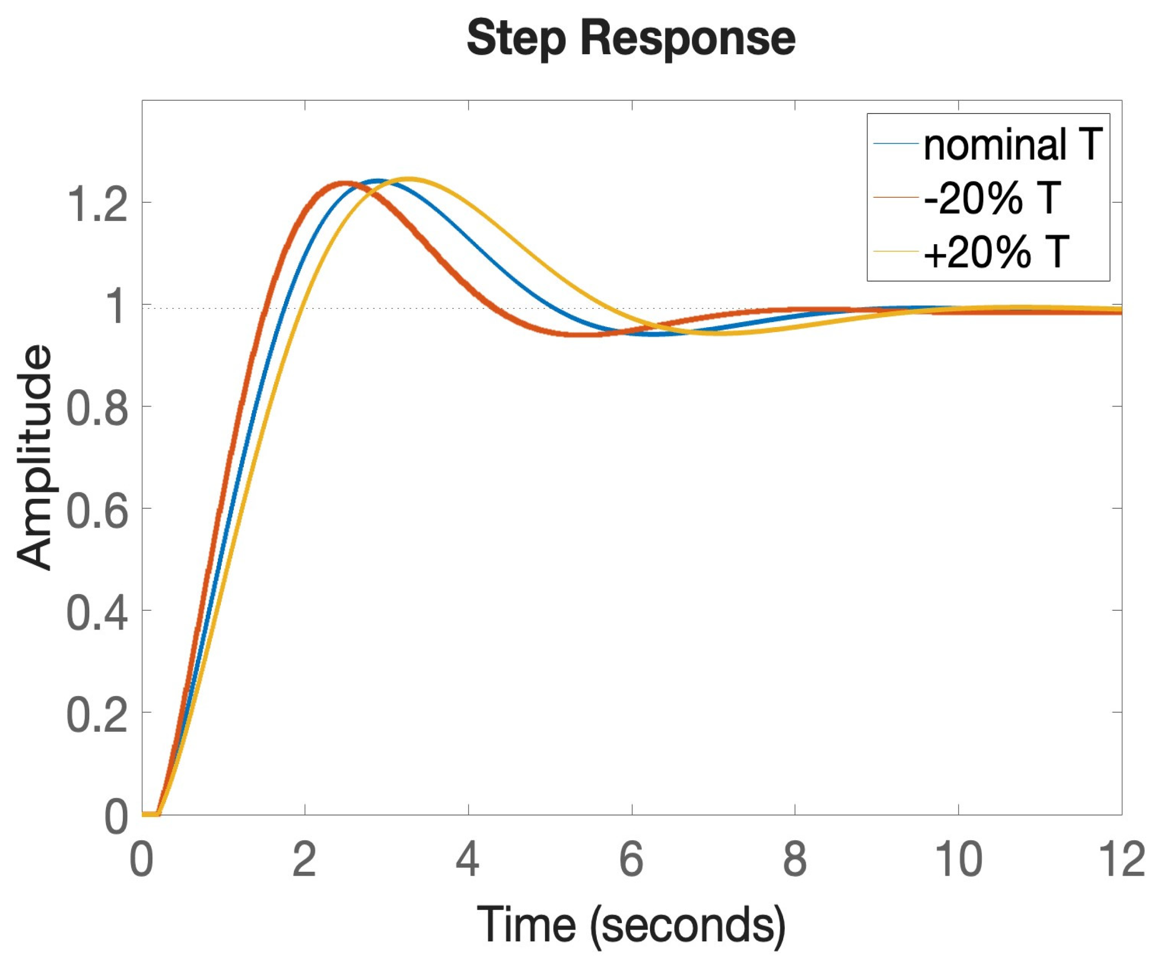
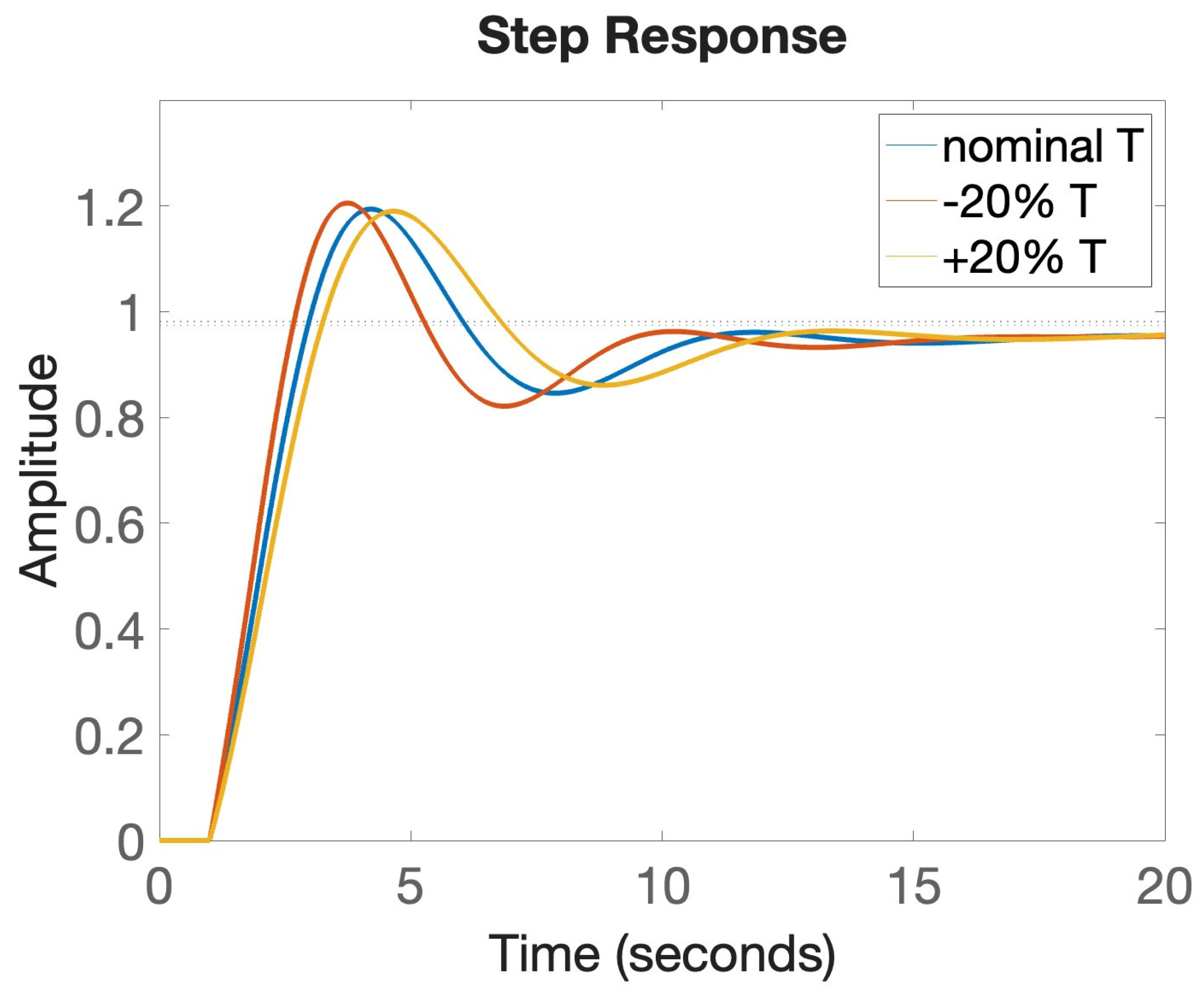
To demonstrate that the PM remains constant despite variations in the time constant, $\pm 20\%$ changes in T are considered next.

Table 2. Robustness results obtained for process P₁(s).

T = 6	${\omega }_c=1$	$\left|L\left(j{\omega }_c\right)\right|$ = 1.0081	PM = 44.81°
T− = 4.8	${\omega }_{c-}=1.15$	$\left|L_{-}\left(j{\omega }_c\right)\right|$ = 1.0158	PM = 44.82°
T+ = 7.2	${\omega }_{c+}=0.89$	$\left|L_{+}\left(j{\omega }_c\right)\right|$ = 1.0058	PM = 44.80°

shows the results obtained. Notice that variations in T have not modified the phase margin of the open-loop system, which is kept constant at approximately 45°, as specified. Hence, the closed-loop overshoot remains the same, at 24%, as indicated in the simulation results in Figure 2.

To implement the controller C(s), a discrete-time approximation of 4th order is obtained using [39] and a sampling period T_s = 0.01 s. The resulting discrete-time controller is:

$$C_1\left(z\right)={\displaystyle \frac{2.55z^4-10.05z^3+ 14.86z^2-9.77z+2.41}{z^4-3.97z^3+5.9z^2-3.91z+0.97}}$$

(34)

For comparative purposes, a standard PI controller is designed to meet the same phase margin and gain crossover frequency as the proposed fractional-order PI. Taking $\lambda$ = 1 in Equation (2) leads to the standard parallel form of the integer order PI controller. Using PM = 45° and ${\omega }_c=1$ rad/s, the proportional and integral gains of the integer order PI controller are computed as: k_p = 4.45 and k_i = 4.15. The closed-loop simulation results using this integer order PI controller are presented in Figure 3. The overshoot in this case ranges from 26% to 33%. The comparison shows the efficiency of the proposed design method and fractional-order controller to ensure the robustness by maintaining the overshoot constant despite time constant variations (as seen in Figure 2).

In terms of settling time, denoted as t_s, the FO-PI reaches steady state within 7.8 s in the nominal case and 6.82 s and 8.74 s for −20% and +20% variation of T, respectively.

Table 3. Closed-loop performance for the process P₁(s) with the proposed FO-PI and the integer order PI controllers.

	FO-PI	PI	FO-PI	PI
T = 6	ISE = 79.8	ISE = 77.8	ts = 7.8	ts = 8.58
T− = 4.8	ISE− = 70	ISE− = 65.1	ts− = 6.82	ts− = 7.21
T+ = 7.2	ISE+ = 88.9	ISE+ = 90.7	ts+ = 8.74	ts+ = 9.65

summarizes these results, as well as those obtained using the PI controller. The results in Table 3 indicate that the FO-PI is faster compared to the traditional PI controller. The Integral of Squared Error (ISE) was also computed, and it is included in Table 3. Although the ISE values do not necessarily favor the use of the FO-PI controller, it is important to note that the main focus of the design was to ensure a constant overshoot, which is clearly evidenced by the results in Table 2 and Figure 2 compared to Figure 3 (where the PI controller is shown).

3.2. Example No. 2

A second example with a larger dead time is considered next, having k = 1, $\tau =1,$ and T = 2:

$$P_2\left(s\right)={\displaystyle \frac{1}{2s+1}}{e}^{-s}$$

(35)

To tune the FO-PI controller, the following performance specifications are used: PM = 45°, ${\omega }_c=0.65$ rad/s and robustness to time constant variations. The algorithm presented in Section 2 yields the results indicated in Figure 4, where e = 0 is obtained for $\lambda =0.6536$. As mentioned before, there is only one solution to Step 6 of the algorithm, clearly visible in Figure 4.

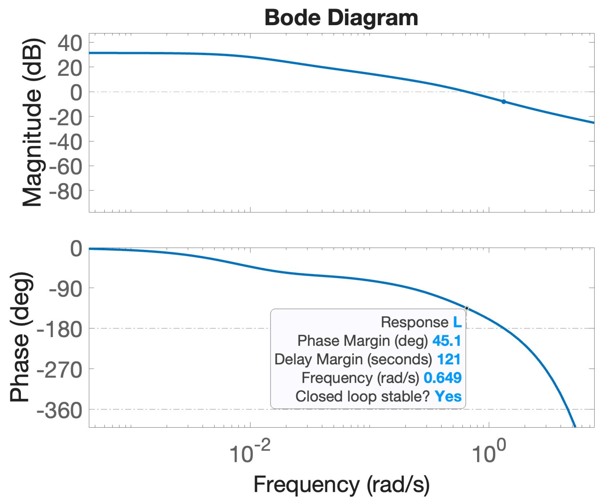
Based on the algorithm, the final results for the tuning of the FO-PI controller are given in

Table 4. Results obtained for process P₂(s).

Step 1	$L\left(j{\omega }_c\right)=-0.7071-j0.7071$
Step 2	$P\left(j{\omega }_c\right)=0.0035-0.6097j$
Step 3	$C\left(j{\omega }_c\right)=1.1531-1.1663j$
Step 4–6	${\lambda }_{min}=0.5036$ $e = 0 \mathrm{for} \lambda =0.6536$ kp = 0.7519 and ki = 1.2966

. The Bode diagram of the open-loop system is shown in Figure 5. The obtained gain crossover frequency and phase margin correspond to the performance specifications.

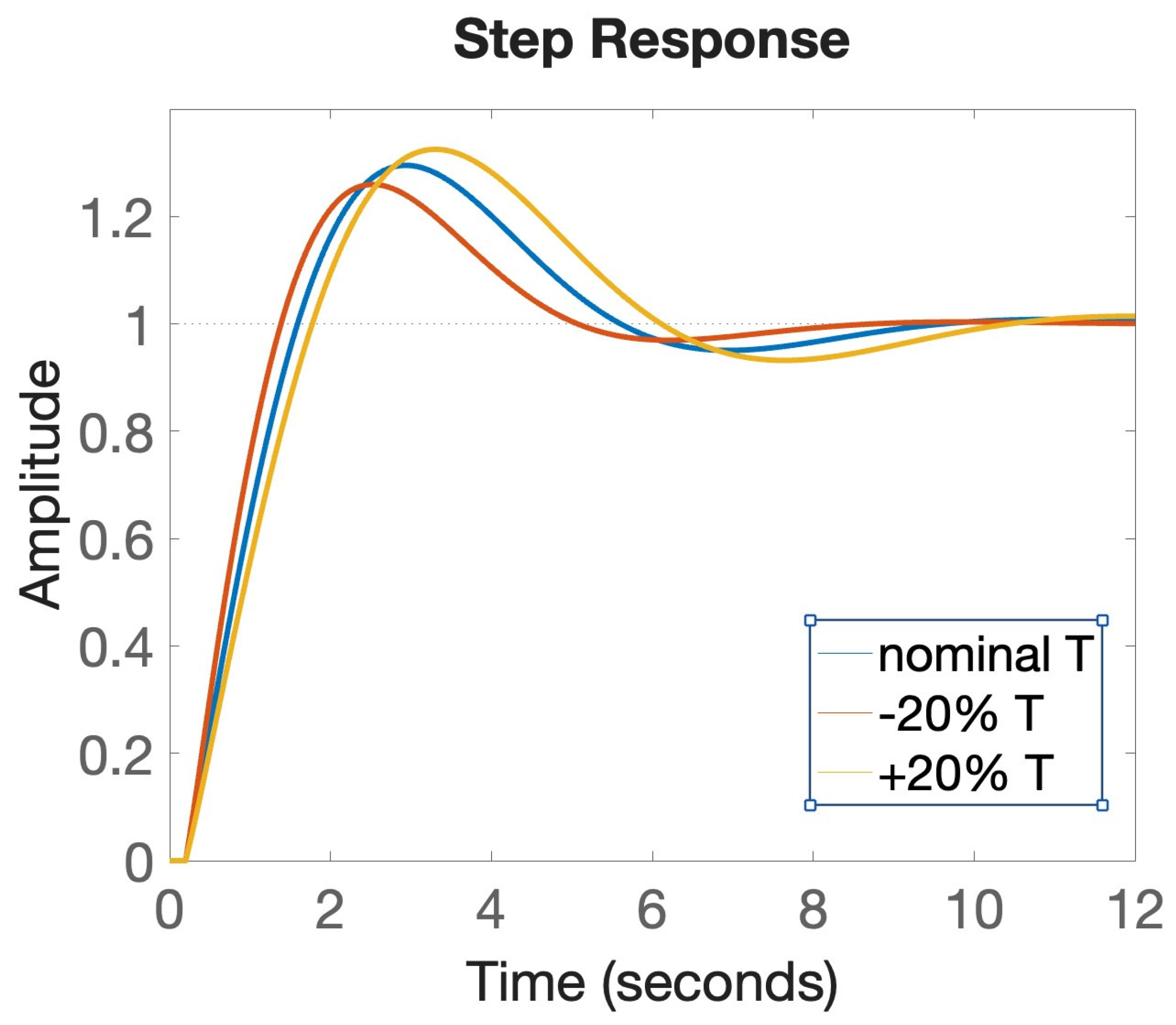
To demonstrate that the PM remains constant despite variations in the time constant, $\pm 20\%$ changes in T are considered next.

Table 5. Robustness results obtained for process P₂(s).

T = 2	${\omega }_c=0.65$	$\left|L\left(j{\omega }_c\right)\right|$ = 0.9985	PM = 45.19°
T− = 1.6	${\omega }_{c-}=0.73$	$\left|L_{-}\left(j{\omega }_c\right)\right|$ = 1.001	PM = 45.24°
T+ = 2.4	${\omega }_{c+}=0.59$	$\left|L_{+}\left(j{\omega }_c\right)\right|$ = 0.9958	PM = 45.02°

shows the results obtained. Notice that variations in T have not modified the phase margin of the open-loop system, which is kept constant at approximately 45°, as specified. Hence, the closed-loop overshoot remains the same, ranging from 18.9–20%, as indicated in the simulation results in Figure 6.

To implement the controller C(s), a discrete-time approximation of 4th order is obtained using [39] and a sampling period T_s = 0.1 s. The discrete-time transfer function of the resulting controller is given as:

$$C_2\left(z\right)={\displaystyle \frac{0.88z^4-3.36z^3+4.84z^2-3.1z+0.74}{z^4-3.94z^3+5.8z^2-3.8z+0.94}}$$

(36)

In terms of settling time, the FO-PI reaches steady state within 10.1 s in the nominal case, 8.91 s, and 11.2 s for −20% and +20% variation of T, respectively. The Integral of Squared Error (ISE) was also computed, yielding an ISE = 16.1 for the nominal value of T, ISE₋ = 15.2, for −20% variation of T, and ISE₊ = 16.9 for a +20% variation of the time constant. It is important to note that obtaining a constant settling time or a small ISE, despite time constant variations, was not the focus of the design; rather, the focus was on obtaining a constant overshot, which is clearly achieved based on the results in Table 5 and Figure 6.

3.3. Example No. 3

A delay-dominant process with k = 1, $\mathit{\tau }\mathbf{=}\mathbf{2}$ and T = 1.1 is considered as the third numerical example:

$${\mathit{P}}_{\mathbf{3}}\left(\mathit{s}\right)\mathbf{=}{\displaystyle \frac{\mathbf{1}}{\mathbf{1.1}\mathit{s}\mathbf{+}\mathbf{1}}}{\mathit{e}}^{\mathbf{-}\mathbf{2}\mathit{s}}$$

(37)

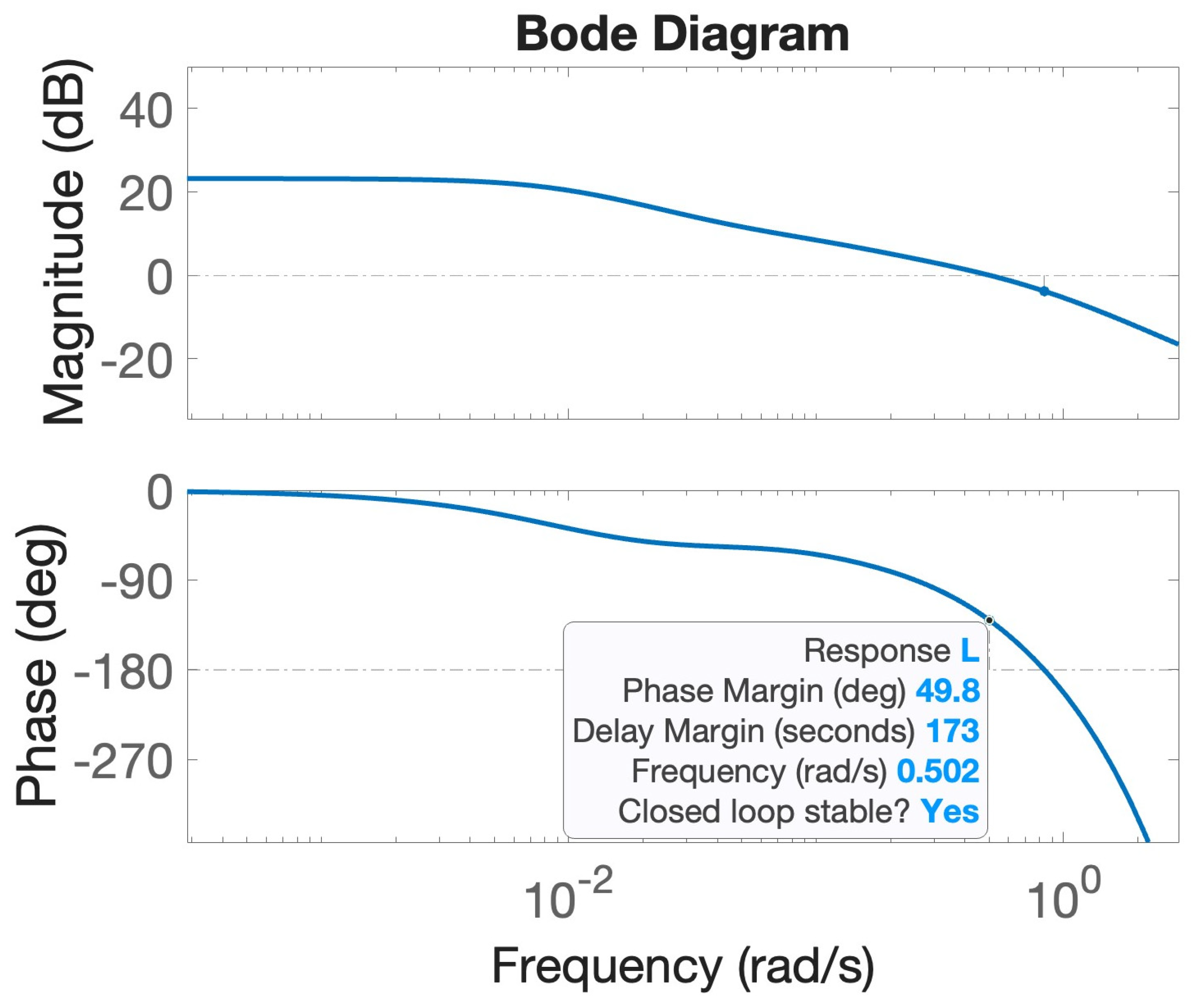
To tune the FO-PI controller, the following performance specifications are used: PM = 50°, ${\mathit{\omega }}_{\mathit{c}}\mathbf{=}\mathbf{0.5}$ rad/s, and robustness to time constant variations. The algorithm presented in Section 2 yields the results indicated in

Table 6. Results obtained for process P₃(s).

Step 1	$L\left(j{\omega }_c\right)=-0.6428-j0.7660$
Step 2	$P\left(j{\omega }_c\right)=0.0595-0.8742j$
Step 3	$C\left(j{\omega }_c\right)=0.8224-0.7913j$
Step 4–6	${\lambda }_{min}=0.4877$ $\mathit{e} = 0 \mathrm{for} \lambda =0.5277$ kp = 0.1526 and ki = 0.6377

. The Bode diagram of the open-loop system is presented in Figure 7. The obtained gain crossover frequency and phase margin correspond to the performance specifications.

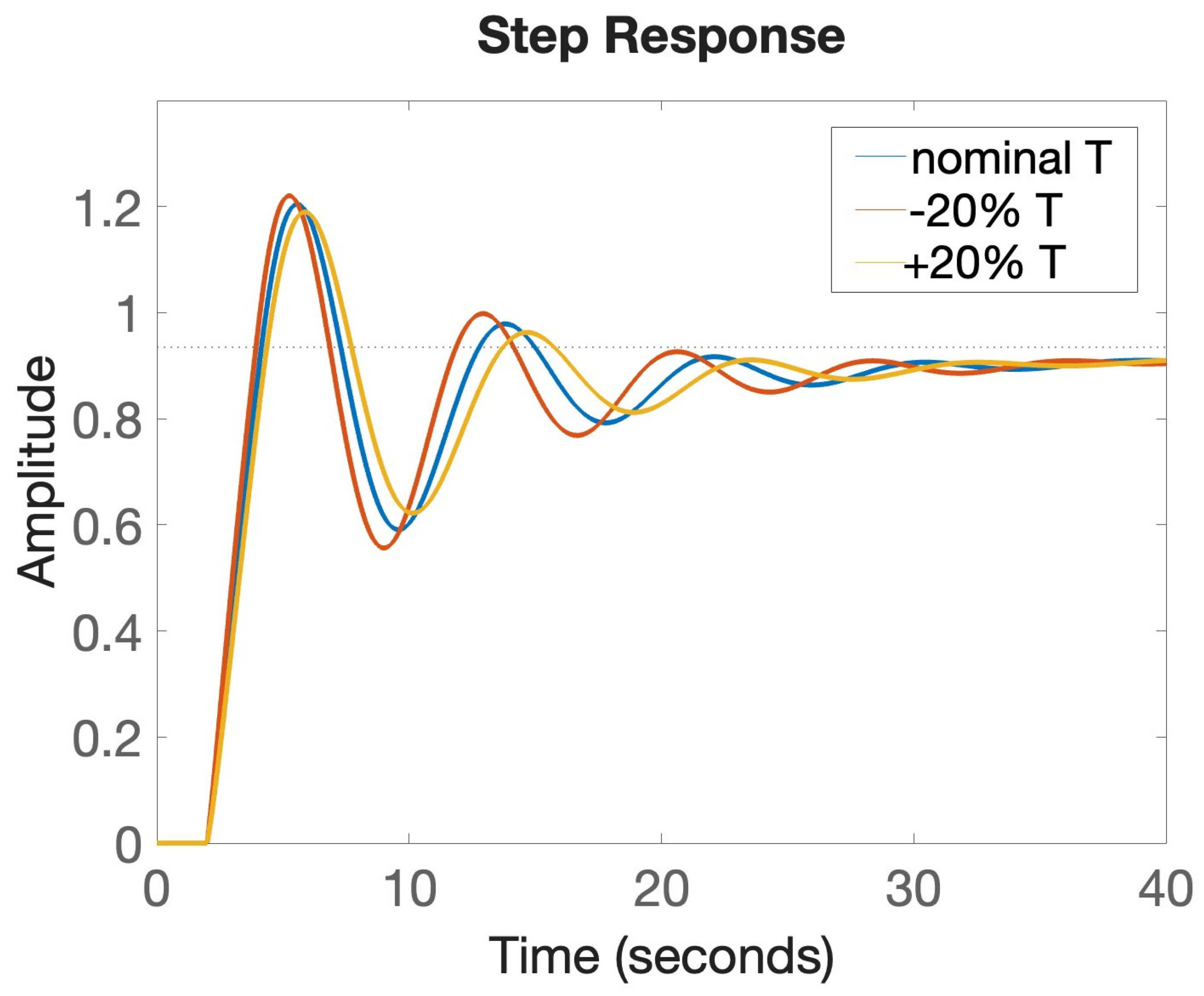
To demonstrate that the PM remains constant despite variations in the time constant, $\mathbf{\pm }\mathbf{20}\mathbf{\%}$ changes in T are considered next.

Table 7. Robustness results obtained for process P₃(s).

T = 1.1	${\omega }_c=0.5$	$\left|L\left(j{\omega }_c\right)\right|$ = 1	PM = 50°
T− = 0.88	${\omega }_{c-}=$0.534	$\left|L_{-}\left(j{\omega }_c\right)\right|$ = 0.9982	PM = 49.98°
T+ = 1.32	${\omega }_{c+}=$0.472	$\left|L_{+}\left(j{\omega }_c\right)\right|$ = 0.9981	PM = 49.89°

shows the results obtained. Notice that variations in T have not modified the phase margin of the open-loop system, which is kept constant at approximately 50°, as specified. Hence, the closed-loop overshoot remains the same, ranging from 19.3–21.5%, as indicated in the simulation results in Figure 8.

To implement the controller C(s), a discrete-time approximation of 4th order is obtained using [39] and a sampling period T_s = 0.1 s. The discrete-time transfer function of the resulting controller is given as:

$$C_3\left(z\right)={\displaystyle \frac{0.41z^4-1.52z^3+2.1z^2-1.28z+0.29}{z^4-3.88z^3+5.63z^2-3.6z+0.88}}$$

(38)

In terms of settling time, the FO-PI reaches steady state within 28.2 s in the nominal case, 26.8 s and 30.1 s for −20% and +20% variation of T, respectively. The Integral of Squared Error (ISE) was also computed, yielding an ISE = 25.95 for the nominal value of T, ISE₋ = 25.85, for −20% variation of T, and ISE₊ = 26.11 for a +20% variation of the time constant. It is important to note that obtaining a constant settling time or a small ISE, despite time constant variations, was not the focus of the design; rather, the focus was on obtaining a constant overshot, which is clearly achieved based on the results in Table 7 and Figure 8.

4. Conclusions

Fractional-order (FO) controllers have gained significant attention over the past 20 years as robust alternatives to traditional PID controllers, with their additional parameters offering enhanced tuning flexibility and system resilience. While most existing methods focus on robustness to gain variations, this paper introduces a novel FO-PI design specifically resilient to time constant variations. By utilizing partial derivatives of the loop frequency response, the proposed approach replaces tedious optimization or graphical-based solutions with a simple 1-step approach. The method is validated using first-order plus dead time processes, ranging from lag- to delay-dominant models. The results presented show that the method is efficient in ensuring the robustness to time constant variations for processes that exhibit a ratio T/τ ranging from 0.55 to 30. The method presented here can be easily extended to higher-order systems and generalized by replacing the corresponding process frequency response in the algorithm. Future work will focus on experimental validation and developing techniques for precise gain crossover frequency and phase margin selection.

References

1. Petráš, I. Chapter Three—Fractional-order control: New control techniques. In Emerging Methodologies and Applications in Modelling, Fractional Order Systems; Radwan, A.G., Khanday, F.A., Said, L.A., Eds.; Academic Press: Cambridge, MA, USA, 2022; Volume 1, pp. 71–106. [Google Scholar] [CrossRef]
2. Tepljakov, A.; Alagoz, B.B.; Yeroglu, C.; Gonzalez, E.A.; Hosseinnia, S.H.; Petlenkov, E.; Ates, A.; Cech, M. Towards Industrialization of FOPID Controllers: A Survey on Milestones of Fractional-Order Control and Pathways for Future Developments. IEEE Access 2021, 9, 21016–21042. [Google Scholar] [CrossRef]
3. Izci, D.; Ekinci, S.; Mohd Tumari, M.Z.; Ahmad, M.A. A Novel Softsign Fractional-Order Controller Optimized by an Intelligent Nature-Inspired Algorithm for Magnetic Levitation Control. Fractal Fract. 2025, 9, 801. [Google Scholar] [CrossRef]
4. Izci, D.; Ekinci, S.; Rizk-Allah, R.M.; Ahmad, M.A. Robust Fractional-Order Control with Master–Slave Mechanism for Motor Speed Regulation. Fractal Fract. 2026, 10, 187. [Google Scholar] [CrossRef]
5. Nataraj, D.; Subramanian, M. Design and optimal tuning of fractional order PID controller for paper machine headbox using jellyfish search optimizer algorithm. Sci. Rep. 2025, 15, 1631. [Google Scholar] [CrossRef]
6. Bashishtha, T.K.; Singh, V.P.; Yadav, U.K.; Sahu, U.K. Fractional-order PID controllers and applications: A comprehensive survey. Annu. Rev. Control 2025, 60, 101013. [Google Scholar] [CrossRef]
7. Jinai, K.; Kawaguchi, N.; Arrieta, O.; Sato, T. Data-Driven Robust Servo Tuning Method Using Fractional-Order PID Controller. IFAC-PapersOnLine 2024, 58, 436–441. [Google Scholar] [CrossRef]
8. Akinwola, A.B.; Alkuhayli, A. Hybrid PSO–Reinforcement Learning-Based Adaptive Virtual Inertia Control for Frequency Stability in Multi-Microgrid PV Systems. Electronics 2025, 14, 3349. [Google Scholar] [CrossRef]
9. Li, X.; Gao, L. Robust Fractional-order PID Tuning Method for a Plant with an Uncertain Parameter. Int. J. Control Autom. Syst. 2021, 19, 1302–1310. [Google Scholar] [CrossRef]
10. Luo, Y.; Chen, Y.Q. Stabilizing and robust fractional order PI controller synthesis for first order plus time delay systems. Automatica 2012, 48, 2159–2167. [Google Scholar] [CrossRef]
11. Dastjerdi, A.A.; Vinagre, B.M.; Chen, Y.Q.; HosseinNia, S.H. Linear fractional order controllers; A survey in the frequency domain. Annu. Rev. Control 2019, 47, 51–70. [Google Scholar] [CrossRef]
12. Birs, I.; Muresan, C.; Nascu, I.; Ionescu, C. A Survey of Recent Advances in Fractional Order Control for Time Delay Systems. IEEE Access 2019, 7, 30951–30965. [Google Scholar] [CrossRef]
13. Ruan, S. Robust Fractional-Order Proportional-Integral Controller Tuning for Load Frequency Control of a Microgrid System with Communication Delay. Energies 2023, 16, 5418. [Google Scholar] [CrossRef]
14. Chen, P.; Luo, Y.; Peng, Y.; Chen, Y.Q. Optimal robust fractional order PIλD controller synthesis for first order plus time delay systems. ISA Trans. 2021, 114, 136–149. [Google Scholar] [CrossRef]
15. Azarmi, R.; Tavakoli-Kakhki, M.; Sedigh, A.K.; Fatehi, A. Robust Fractional Order PI Controller Tuning Based on Bode’s Ideal Transfer Function. IFAC-PapersOnLine 2016, 49, 158–163. [Google Scholar] [CrossRef]
16. Zheng, W.; Luo, Y.; Chen, Y.; Wang, X. A Simplified Fractional Order PID Controller’s Optimal Tuning: A Case Study on a PMSM Speed Servo. Entropy 2021, 23, 130. [Google Scholar] [CrossRef]
17. Liu, L.; Zhang, S. Robust Fractional-Order PID Controller Tuning Based on Bode’s Optimal Loop Shaping. Complexity 2018, 2018, 6570560. [Google Scholar] [CrossRef]
18. Sánchez, H.S.; Padula, F.; Visioli, A.; Vilanova, R. Tuning rules for robust FOPID controllers based on multi-objective optimization with FOPDT models. ISA Trans. 2017, 66, 344–361. [Google Scholar] [CrossRef]
19. Şenol, B.; Demiroğlu, U. Fractional order proportional derivative control for first order plus time delay plants: Achieving phase and gain specifications simultaneously. Trans. Inst. Meas. Control 2019, 41, 4358–4369. [Google Scholar] [CrossRef]
20. Saxena, S.; Hote, Y.V. Design of robust fractional-order controller using the Bode ideal transfer function approach in IMC paradigm. Nonlinear Dyn. 2022, 107, 983–1001. [Google Scholar] [CrossRef]
21. Wu, Z.; Li, D.; Xue, Y.; He, T.; Zheng, S. Tuning for Fractional Order PID Controller based on Probabilistic Robustness. IFAC-PapersOnLine 2018, 51, 675–680. [Google Scholar] [CrossRef]
22. Kumar, V.; Rana, K.P.S.; Mishra, P. Robust speed control of hybrid electric vehicle using fractional order fuzzy PD and PI controllers in cascade control loop. J. Frankl. Inst. 2016, 353, 1713–1741. [Google Scholar] [CrossRef]
23. Monje, C.; Calderon, A.; Vinagre, B.; Chen, Y.; Feliu, V. On Fractional PIλ Controllers: Some Tuning Rules for Robustness to Plant Uncertainties. Nonlinear Dyn. 2004, 38, 369–381. [Google Scholar] [CrossRef]
24. Pachauri, N.; Thangavel, V.; Suresh, V.; Kantipudi, M.P.; Kotb, H.; Tripathi, R.N.; Bajaj, M. A Robust Fractional-Order Control Scheme for PV-Penetrated Grid-Connected Microgrid. Mathematics 2023, 11, 1283. [Google Scholar] [CrossRef]
25. Martins-Gomes, M.C.; Ayres, F.A.d.C., Jr.; da Costa, C.T., Jr.; de Bessa, I.V.; Farias, N.J.d.S.; de Medeiros, R.L.P.; Silva, L.E.S.; de Lucena, V.F., Jr. Fractional-order robust control design under parametric uncertain approach. ISA Trans. 2024, 153, 420–432. [Google Scholar] [CrossRef]
26. Feliu-Batlle, V. Robust isophase margin control of oscillatory systems with large uncertainties in their parameters: A fractional-order control approach. Int. J. Robust. Nonlinear Control 2017, 27, 2145–2164. [Google Scholar] [CrossRef]
27. Mihaly, V.; Şuşcă, M.; Dulf, E.H.; Morar, D.; Dobra, P. Fractional Order Robust Controller for Fractional-Order Interval Plants. IFAC-PapersOnLine 2022, 55, 151–156. [Google Scholar] [CrossRef]
28. Gao, Z. Robust stabilization criterion of fractional-order controllers for interval fractional-order plants. Automatica 2015, 61, 9–17. [Google Scholar] [CrossRef]
29. Lanusse, P.; Malti, R.; Melchior, P. CRONE control system design toolbox for the control engineering community: Tutorial and case study. Philos. Trans. A Math. Phys. Eng. Sci. 2013, 371, 20120149. [Google Scholar] [CrossRef]
30. Mseddi, A.; Abid, A.; Naifar, O.; Rhaima, M.; Ben Makhlouf, A.; Mchiri, L. Investigation of the robust fractional order control approach associated with the online analytic unity magnitude shaper: The case of wind energy systems. Fractal Fract. 2024, 8, 187. [Google Scholar] [CrossRef]
31. Rhouma, A.; Hafsi, S.; Laabidi, K. Stabilizing and Robust Fractional PID Controller Synthesis for Uncertain First-Order plus Time-Delay Systems. Math. Probl. Eng. 2021, 2021, 9940634. [Google Scholar] [CrossRef]
32. Jin, Y.; Chen, Y.-Q.; Xue, D. Time-constant robust analysis of a fractional order [proportional derivative] controller. IET Control Theory Appl. 2011, 5, 164–172. [Google Scholar] [CrossRef]
33. Beschi, M.; Padula, F.; Visioli, A. The generalised isodamping approach for robust fractional PID controllers design. Int. J. Control 2015, 90, 1157–1164. [Google Scholar] [CrossRef]
34. Badri, V.; Tavazoei, M.S. On time-constant robust tuning of fractional order proportional derivative controllers. IEEE/CAA J. Autom. Sin. 2019, 6, 1179–1186. [Google Scholar] [CrossRef]
35. Badau, N.E.; Popescu, T.M.; Mihai, M.D.; Birs, I.R.; Muresan, C.I. A Robust Fractional-Order Controller for Biomedical Applications. Fractal Fract. 2025, 9, 597. [Google Scholar] [CrossRef]
36. Muresan, C.I.; Mihai, M.D.; Hegedus, E.T.; Badau, N.; Birs, I.R.; De Keyser, R. A Robust fractional order PI controller for time constant variations. Fract. Calc. Appl. Anal. 2026, 29, 980–1005. [Google Scholar] [CrossRef]
37. Badau, N.E.; Tudor, A.M.; Muresan, C.I. Experimental Validation of a Robust [FO-PID]λ Controller. Mathematics 2026, 14, 592. [Google Scholar] [CrossRef]
38. Åström, K.J.; Hägglund, T. Advanced PID Control; ISA—The Instrumentation, Systems, and Automation Society: Research Triangle Park, NC, USA, 2006; ISBN 978-1-55617-942-6. [Google Scholar]
39. De Keyser, R.; Muresan, C.I.; Ionescu, C.M. An efficient algorithm for low-order direct discrete-time implementation of fractional order transfer functions. ISA Trans. 2018, 74, 229–238. [Google Scholar] [CrossRef] [PubMed]
Figure 1. The Bode diagram of the loop frequency response for P1(s).
Fractalfract 10 00330 g001
Figure 2. Closed-loop simulation results for P1(s).
Fractalfract 10 00330 g002
Figure 3. Closed-loop simulation results for P1(s) using an integer order PI controller.
Fractalfract 10 00330 g003
Figure 4. The error e = λ n e w λ as a function of λ for designing the controller for P2(s).
Fractalfract 10 00330 g004
Figure 5. The Bode diagram of the loop frequency response for P2(s).
Fractalfract 10 00330 g005
Figure 6. Closed-loop simulation results for P2(s).
Fractalfract 10 00330 g006
Figure 7. The Bode diagram of the loop frequency response for P3(s).
Fractalfract 10 00330 g007
Figure 8. Closed-loop simulation results for P3(s).
Fractalfract 10 00330 g008