A Space–Time Spectral Method for Nonlinear Fractional Convection–Diffusion Equations with Viscosity Terms

Abstract

We develop a high-order space-time spectral method for nonlinear convection–diffusion equations with a Riemann–Liouville time-fractional derivative and a spectrally defined space-fractional Laplacian. The spatial discretization uses a Fourier spectral method that diagonalizes the fractional Laplacian under periodic boundary conditions. The temporal discretization employs a Petrov–Galerkin method based on generalized Jacobi functions which capture the initial singularity exactly. The nonlinear convection term is treated pseudo-spectrally, and the resulting algebraic system is solved with a damped Newton iteration. Rigorous error analysis proves exponential convergence in both space and time. Numerical experiments for various fractional orders confirm the spectral accuracy. Simulations of the fractional Burgers equation demonstrate that increasing the viscosity enhances diffusion and stabilizes the solution, while a nonlinear coefficient that significantly exceeds the viscosity leads to error growth over long time intervals. The method provides an efficient and accurate tool for simulating anomalous transport phenomena.

1. Introduction

Fractional differential equations have emerged as a powerful modeling framework for complex physical systems characterized by memory effects and long-range interactions. By incorporating fractional-order derivatives, these models capture anomalous transport phenomena that elude traditional integer-order formulations. Time-fractional derivatives naturally describe history-dependent processes, such as viscoelastic relaxation, signal propagation in heterogeneous media, and turbulent flows, while space-fractional Laplacians account for nonlocal diffusion observed in porous media transport, groundwater contaminant spreading, and plasma turbulence [1]. The interplay between nonlinear convection and fractional diffusion gives rise to a rich class of space-time fractional convection–diffusion equations, which serve as the foundation for this work. Such models find broad applicability across diverse fields: in fluid dynamics, fractional Burgers-type equations capture the cumulative effect of wall friction through boundary layers and the unidirectional propagation of weakly nonlinear acoustic waves [2,3]; in environmental engineering, fractional convection–dispersion equations successfully describe non-Fickian transport in heterogeneous aquifers where contaminant plumes exhibit heavy-tailed breakthrough curves [4]; in materials science, time-fractional constitutive relations model stress relaxation in viscoelastic polymers while space-fractional terms incorporate long-range elastic interactions [5]; and in plasma physics, fractional models accurately characterize anomalous particle transport in fusion devices where standard diffusion theories fall short [6].

A significant body of literature has been devoted to the numerical treatment of fractional convection–diffusion equations. Finite difference methods remain the most widely used approach due to their conceptual simplicity and ease of implementation. Recent advances include semi-adaptive finite difference schemes for two-sided fractional quenching problems [7], exponentially fitted methods for singularly perturbed time-fractional convection–diffusion problems with variable coefficients [8], and explicit group methods for solving two-dimensional time-fractional Burgers equations [9]. Finite element methods have also attracted considerable attention. For instance, a stabilized finite element formulation with shock-capturing has been developed for advection-dominated convection–diffusion equations involving time-fractional derivatives [10], where nonlinear systems are solved using the Newton–Raphson method at each time step. Finite element algorithms based on high-order time approximation have been proposed for time-fractional convection–diffusion equations [11], while the finite volume element method has been applied to two-dimensional space-fractional convection–diffusion problems [4]. Meshfree and spectral methods have also been actively explored. The corrected smoothed particle hydrodynamics (CSPH) method has been coupled with numerical integration techniques for solving multi-dimensional space-fractional convection–diffusion equations with Riemann–Liouville derivatives [12], and radial basis function (RBF) finite difference approaches have been applied to generalized time-fractional Burgers equations under various boundary conditions [13]. In the spectral realm, Müntz spectral methods have been proposed for two-dimensional space-fractional convection–diffusion equations [14], and spectral Galerkin methods have been applied to Riesz space-fractional convection–diffusion equations [15]. Petrov–Galerkin spectral methods have been developed for fractional convection–diffusion equations with two-sided fractional derivatives [16]. A barycentric rational interpolation method has been employed to solve time-dependent fractional convection–diffusion equations [17], leveraging spectral techniques to handle the nonlocal nature of fractional operators.

Despite the availability of these numerical approaches, several fundamental challenges remain unresolved when solving space-time fractional nonlinear convection–diffusion equations of the form considered here. First, the Riemann–Liouville time-fractional derivative introduces a weak singularity at the initial time $t=0$, where typical solutions behave as $t^{\alpha }$ times a smooth function. Standard polynomial or spline approximations fail to capture this singular behavior efficiently, leading to reduced convergence rates unless the grid is heavily refined near $t=0$ [18]. Second, the spectrally defined space-fractional Laplacian ${(-\Delta )}^{\beta /2}$ is a nonlocal pseudodifferential operator that becomes dense in any polynomial basis, rendering standard finite element or finite difference methods computationally expensive due to the resulting dense linear systems [19]. Third, the nonlinear convection term $\nabla ·\mathbf{F}\left(u\right)$ couples all Fourier modes, complicating the solution process and requiring careful treatment to maintain both stability and accuracy [20]. Fourth, the space-time coupled nature of the problem demands a discretization strategy that simultaneously addresses spatial and temporal fractional operators in a balanced manner to achieve exponential convergence overall.

To overcome these challenges, this paper proposes a novel space-time spectral method that combines a Fourier spectral discretization in space with a Petrov–Galerkin spectral method based on generalized Jacobi functions (GJFs) in time [18,21,22]. The Fourier spectral method diagonalizes the spectral fractional Laplacian exactly, reducing the spatial discretization to a set of decoupled algebraic equations for each Fourier mode. This approach completely avoids the dense matrix fill-in typically associated with nonlocal operators. For the temporal direction, generalized Jacobi functions of the form ${\psi }_m\left(t\right)={(t/T)}^{\alpha }{P}_m^{(\alpha ,0)}(2t/T-1)$ are employed as trial functions. The factor ${(t/T)}^{\alpha }$ exactly captures the initial singularity of the solution, and a key property, the closure under Riemann–Liouville fractional differentiation, ensures that the time stiffness matrix is diagonal, dramatically simplifying the implementation. The nonlinear convection term is treated pseudo-spectrally using fast Fourier transforms (FFTs) and high-order Gauss–Legendre quadrature, achieving spectral accuracy in both space and time while maintaining computational efficiency. The resulting fully discrete nonlinear algebraic system is solved by Newton’s method with a matrix-free Krylov subspace solver.

A typical model equation on a periodic domain $\Omega ={[0,2\pi )}^2$ takes the form

$${}_0{}^{RL}D_t^{\alpha }u(\mathbf{x},t)+{\mu }_{\mathrm{nl}}\nabla ·\mathbf{F}\left(u\right)=-\nu {(-\Delta )}^{\beta /2}u(\mathbf{x},t)+f(\mathbf{x},t),\mathbf{x}=(x,y)\in \Omega ,t\in (0,T],$$

(1)

supplemented with periodic boundary conditions

$$\begin{array}{c}\hfill u(x+2\pi ,y,t)=u(x,y+2\pi ,t)=u(x,y,t),(x,y)\in {\mathbb{R}}^2,t>0,\end{array}$$

(2)

and an appropriate initial condition for the Riemann–Liouville derivative of order $\alpha -1$

$$\begin{array}{c}\hfill {}_0{}^{RL}D_t^{\alpha -1}u(\mathbf{x},0)=u_0\left(\mathbf{x}\right),\mathbf{x}=(x,y)\in \Omega .\end{array}$$

(3)

Here, ${}_0{}^{RL}D_t^{\alpha }$ denotes the left-sided Riemann–Liouville fractional derivative of order $\alpha \in (0,1)$, ∇ represents the gradient operator defined as $\nabla =({\partial }_x,{\partial }_y)$, and $\mathbf{F}\left(u\right)=(u^2/2,u^2/2)$ gives the nonlinear convection so that

$$\begin{array}{c}\hfill \nabla ·\mathbf{F}\left(u\right)=({\partial }_x,{\partial }_y)·\left({\displaystyle \frac{u^2}{2}},{\displaystyle \frac{u^2}{2}}\right)=u{\partial }_{x}u+u{\partial }_{y}u.\end{array}$$

The parameter ${\mu }_{\mathrm{nl}}$ controls the strength of the nonlinear convection. When ${\mu }_{\mathrm{nl}}=0$, the equation becomes linear; when ${\mu }_{\mathrm{nl}}=1$, we recover the standard nonlinear Burgers equation. $\nu >0$ is the viscosity coefficient, and ${(-\Delta )}^{\beta /2}$ is the spectral fractional Laplacian with $\beta \in (1,2)$ defined via Fourier series

$${(-\Delta )}^{\beta /2}u\left(\mathbf{x}\right)=\sum _{\mathbf{k}\in {\mathbb{Z}}^2}{\left|\mathbf{k}\right|}^{\beta }{\widehat{u}}_{\mathbf{k}}{e}^{i\mathbf{k}·\mathbf{x}},\beta \in (1,2).$$

for $u\left(\mathbf{x}\right)={\sum }_{\mathbf{k}\in {\mathbb{Z}}^2}{\widehat{u}}_{\mathbf{k}}{e}^{i\mathbf{k}·\mathbf{x}}$, with $\mathbf{k}=(k_1,k_2)$, and $\left|\mathbf{k}\right|=\sqrt{k_1^2+k_2^2}$, $\mathbb{Z}$ denotes the set of all integers. The source term f is assumed to be smooth. In all theoretical derivations in Section 2, Section 3 and Section 4, we keep ${\mu }_{\mathrm{nl}}=1$ without loss of generality, but the numerical experiments in Section 5 explicitly vary ${\mu }_{\mathrm{nl}}$ to examine its effect on the solution.

Numerically, solving such equations faces two major challenges:

(i)

The time-fractional derivative introduces a weak singularity at $t=0$;

(ii)

The space-fractional Laplacian is a nonlocal operator that becomes dense in a standard polynomial basis.

In this work, we address these issues by combining a Fourier spectral method for the spatial discretization with a generalized Jacobi function (GJF) spectral method in time within a Petrov–Galerkin framework [18,21,22], which exactly captures the initial singularity and yields exponential convergence. The nonlinear convection term is treated by a pseudo-spectral collocation technique, and the resulting algebraic system is solved by Newton’s method. The primary contributions of this work are threefold. First, we provide a comprehensive derivation of the space-time spectral method for nonlinear fractional convection–diffusion equations, including the construction of basis functions, the variational formulation, and the pseudo-spectral evaluation of nonlinear terms. Second, we present a detailed error analysis that rigorously establishes exponential convergence in both space and time under appropriate analyticity assumptions on the solution. Third, we offer a complete algorithmic framework with pseudo-code, making the method readily implementable by researchers in the field.

The remainder of this paper is structured as follows. Section 2 presents the necessary preliminaries on Riemann–Liouville fractional derivatives, spectral fractional Laplacians, generalized Jacobi functions, and relevant function spaces. Section 3 describes the fully discrete numerical scheme, including spatial Fourier discretization, temporal GJF discretization, pseudo-spectral treatment of the nonlinear convection term, and the Newton–Krylov solver. Section 4 provides a rigorous error analysis, establishing exponential convergence. Section 5 presents the numerical results, and Section 6 shows the concluding remarks and outlines directions for future work.

2. Preliminaries

We recall the definitions and key properties of Riemann–Liouville fractional derivatives, spectral fractional Laplacians, and generalized Jacobi functions.

2.1. Riemann–Liouville Fractional Derivative

For $\alpha \in (0,1)$ and a function $u\in L^1(0,T)$, the left-sided Riemann–Liouville fractional derivative is defined by [23]

$${}_0{}^{RL}D_t^{\alpha }u\left(t\right)={\displaystyle \frac{1}{\mathrm{\Gamma }(1-\alpha )}}{\displaystyle \frac{d}{dt}}{\int }_0^t{(t-s)}^{-\alpha }u\left(s\right)ds.$$

A crucial property for our analysis is its action on power functions:

$${}_0{}^{RL}D_t^{\alpha }{t}^{\gamma }={\displaystyle \frac{\mathrm{\Gamma }(\gamma +1)}{\mathrm{\Gamma }(\gamma -\alpha +1)}}{t}^{\gamma -\alpha },\gamma >-1.$$

Thus, for a function that behaves like $t^{\alpha }$ times a smooth function near $t=0$, its Riemann–Liouville fractional derivative remains bounded at the origin. In fact, for the power function $t^{\gamma }$ with $\gamma >-1$, the derivative is proportional to $t^{\gamma -\alpha }$, which is bounded near $t=0$ if and only if $\gamma \ge \alpha$.

2.2. Spectral Fractional Laplacian

On the domain $\Omega ={[0,2\pi )}^2$ with periodic boundary conditions, the spectral fractional Laplacian of order $\beta /2$ is defined via Fourier series [24]. For $u\left(\mathbf{x}\right)={\sum }_{\mathbf{k}\in {\mathbb{Z}}^2}{\widehat{u}}_{\mathbf{k}}{e}^{i\mathbf{k}·\mathbf{x}}$,

$${(-\Delta )}^{\beta /2}u\left(\mathbf{x}\right)=\sum _{\mathbf{k}\in {\mathbb{Z}}^2}{\left|\mathbf{k}\right|}^{\beta }{\widehat{u}}_{\mathbf{k}}{e}^{i\mathbf{k}·\mathbf{x}},\left|\mathbf{k}\right|=\sqrt{k_1^2+k_2^2},\beta \in (1,2).$$

For a periodic function $u\left(\mathbf{x}\right)$ on $\Omega ={[0,2\pi )}^2$, its Fourier coefficients are given by

$${\widehat{u}}_{\mathbf{k}}={\displaystyle \frac{1}{{\left(2\pi \right)}^2}}{\int }_{\Omega }u\left(\mathbf{x}\right)e^{-i\mathbf{k}·\mathbf{x}}d\mathbf{x},\mathbf{k}\in {\mathbb{Z}}^2.$$

(4)

If $u(·,t)\in H^s(\Omega )$ with $s>1$, the Fourier series converges uniformly and $|{\widehat{u}}_{\mathbf{k}}{\left(t\right)|\le C|\mathbf{k}|}^{-s}$; for an analytic u, the convergence is exponential.

The spectral fractional Laplacian ${(-\Delta )}^{\beta /2}$ ($\beta \in (1,2)$) is defined by its action on Fourier modes:

$${(-\Delta )}^{\beta /2}{e}^{i\mathbf{k}·\mathbf{x}}={\left|\mathbf{k}\right|}^{\beta }{e}^{i\mathbf{k}·\mathbf{x}}.$$

(5)

By linearity, for any $u\left(\mathbf{x}\right)={\sum }_{\mathbf{k}\in {\mathbb{Z}}^2}{\widehat{u}}_{\mathbf{k}}{e}^{i\mathbf{k}·\mathbf{x}}$,

$${(-\Delta )}^{\beta /2}u\left(\mathbf{x}\right)=\sum _{\mathbf{k}\in {\mathbb{Z}}^2}{\left|\mathbf{k}\right|}^{\beta }{\widehat{u}}_{\mathbf{k}}{e}^{i\mathbf{k}·\mathbf{x}}.$$

(6)

This definition is standard and agrees with the Riesz potential definition on the torus [24]. It is diagonal in the Fourier basis, which is crucial for the efficiency of our method.

2.3. Generalized Jacobi Functions

Let $T>0$. Mapping $[0,T]$ to $[-1,1]$ by $s=2t/T-1$, the generalized Jacobi functions are defined as [18]

$${\psi }_m\left(t\right)={\left({\displaystyle \frac{2t}{T}}\right)}^{\alpha }{P}_m^{(\alpha ,0)}\left(s\right),m=0,1,\dots ,N_t,$$

(7)

where $P_m^{(\alpha ,0)}$ are Jacobi polynomials. The factor ${(2t/T)}^{\alpha }$ captures the initial singularity of solutions to fractional differential equations. Since the initial singularity occurs only at $t=0$, we set the second Jacobi parameter to 0; the weight ${(1-s)}^{\alpha }$ then exactly matches the singular behavior. The admissible range of the time-fractional order is $\alpha \in (0,1)$, which corresponds to a fractional derivative of order $\alpha$. For other types of singularities, different parameters $(\alpha ,\beta )$ could be used, but they are not required in this work. We take the test functions as Legendre polynomials for the Petrov–Galerkin method as

$${\varphi }_n\left(t\right)=P_n^{(0,0)}\left(s\right)=L_n\left(s\right),n=0,\dots ,N_t.$$

(8)

A key property is the closure under fractional differentiation:

$${}_0{}^{RL}D_t^{\alpha }{\psi }_m\left(t\right)={\displaystyle \frac{\mathrm{\Gamma }(m+\alpha +1)}{\mathrm{\Gamma }(m+1)}}{\left({\displaystyle \frac{2}{T}}\right)}^{\alpha }{\varphi }_m\left(t\right).$$

(9)

This relation follows from the identity for fractional derivatives of Jacobi polynomials and implies that the time stiffness matrix is diagonal.

2.4. Function Spaces and Projections

For the error analysis we use the weighted space $L_{\omega }^2(0,T)$ with $\omega \left(t\right)=t^{\alpha }$. The Fourier projection $P_K$ onto the space ${\mathbb{P}}_K=span\{e^{i\mathbf{k}·\mathbf{x}}: |k_1|\le K_1,|k_2|\le K_2\}$ satisfies, for analytic functions [25],

$$\begin{array}{c}\hfill \parallel u-P_K{u\parallel }_{L^2(\Omega )}\le C{e}^{-c{K}_{min}},K_{min}=min(K_1,K_2).\end{array}$$

(10)

The space-time norm is defined as

$${\parallel u\parallel }_{L_{\omega }^2(I;L^2(\Omega ))}={\left({\int }_0^T{\parallel u(·,t)\parallel }_{L^2(\Omega )}^2\omega \left(t\right)dt\right)}^{1/2}.$$

These preliminaries provide the necessary tools for constructing the fully discrete scheme in the next section.

3. Fully Discrete Numerical Scheme

In this section we develop the full discretization of the model problem (1). We first discretize the spatial derivatives using a Fourier spectral method, which diagonalizes the fractional Laplacian. Then, we apply a Petrov–Galerkin spectral method in time using generalized Jacobi functions to handle the Riemann–Liouville fractional derivative and the initial singularity. The nonlinear convection term is treated pseudo-spectrally, and the resulting algebraic system is solved by Newton’s method combined with a Krylov subspace solver.

3.1. Spatial Discretization: Fourier Spectral Method

We consider periodic boundary conditions on $\Omega ={[0,2\pi )}^2$. The solution is approximated by a truncated Fourier series

$$u_N(\mathbf{x},t)=\sum _{\mathbf{k}\in \mathcal{K}}{\widehat{u}}_{\mathbf{k}}\left(t\right)e^{i\mathbf{k}·\mathbf{x}},\mathcal{K}=\{(k_1,k_2): |k_1| \le K_1,|k_2| \le K_2\},$$

with $N_x=2K_1+1$, $N_y=2K_2+1$ grid points. The Fourier coefficients ${\widehat{u}}_{\mathbf{k}}\left(t\right)$ depend on time. The spectral fractional Laplacian acts diagonally:

$$\begin{array}{c}\hfill {(-\Delta )}^{\beta /2}{u}_N(\mathbf{x},t)=\sum _{\mathbf{k}\in \mathcal{K}}{\left|\mathbf{k}\right|}^{\beta }{\widehat{u}}_{\mathbf{k}}\left(t\right)e^{i\mathbf{k}·\mathbf{x}}.\end{array}$$

(11)

Partial derivatives are also diagonal as ${\partial }_{x_j}{u}_N=\sum i{k}_j{\widehat{u}}_{\mathbf{k}}{e}^{i\mathbf{k}·\mathbf{x}}$.

3.2. Temporal Discretization: GJF–Petrov–Galerkin Method

To capture the weak singularity of the solution at $t=0$, which is caused by the Riemann–Liouville derivative, we employ a Petrov–Galerkin spectral method in time using generalized Jacobi functions. Define the affine mapping $s=2t/T-1$ from $[0,T]$ to $[-1,1]$. The trial functions are

$${\psi }_m\left(t\right)={\left({\displaystyle \frac{2t}{T}}\right)}^{\alpha }{P}_m^{(\alpha ,0)}\left(s\right),m=0,\dots ,N_t,$$

where $P_m^{(\alpha ,0)}$ are Jacobi polynomials. The test functions are Legendre polynomials:

$${\varphi }_n\left(t\right)=P_n^{(0,0)}\left(s\right),n=0,\dots ,N_t.$$

The trial space is ${\mathcal{U}}_{N_t}=span\left\{{\psi }_m\right\}$, and the test space is ${\mathcal{V}}_{N_t}=span\left\{{\varphi }_n\right\}$. A key property is the closure under the fractional derivative:

$${}_0{}^{RL}D_t^{\alpha }{\psi }_m\left(t\right)={\displaystyle \sum _{n=0}^m}{d}_{mn}^{\left(\alpha \right)}{\varphi }_n\left(t\right),$$

where the coefficients $d_{mn}^{\left(\alpha \right)}$ can be computed explicitly [18].

We then define the time mass and stiffness matrices:

$$\begin{array}{cc}\hfill M_{nm}^t& ={\langle {\psi }_m,{\varphi }_n\rangle }_t={\int }_0^T{\psi }_m\left(t\right){\varphi }_n\left(t\right)dt,\hfill \end{array}$$

(12)

$$\begin{array}{cc}\hfill K_{nm}^t& ={\langle {}_0{}^{RL}D_t^{\alpha }{\psi }_m,{\varphi }_n\rangle }_t={\displaystyle \sum _{l=0}^m}{d}_{lm}^{\left(\alpha \right)}{\langle {\varphi }_l,{\varphi }_n\rangle }_t.\hfill \end{array}$$

(13)

Since ${\langle {\varphi }_l,{\varphi }_n\rangle }_t={\displaystyle \frac{T}{2}}{\displaystyle \frac{2}{2n+1}}{\delta }_{ln}$, the matrix $K^t$ is upper triangular and can be computed once.

3.3. Space-Time Variational Formulation

We seek the fully discrete solution

$$u_{KN}(\mathbf{x},t)=\sum _{\mathbf{k}\in \mathcal{K}}{\displaystyle \sum _{m=0}^{N_t}}{\widehat{u}}_{\mathbf{k},m}{e}^{i\mathbf{k}·\mathbf{x}}{\psi }_m\left(t\right),$$

(14)

such that for all ${\mathbf{k}}^{\prime }\in \mathcal{K}$ and $n=0,1,\dots ,N_t$,

$${\int }_0^T{\int }_{\Omega }({}_0{}^{RL}D_t^{\alpha }{u}_{KN}+\nabla ·\mathbf{F}\left(u_{KN}\right)+\nu {(-\Delta )}^{\beta /2}{u}_{KN}-f)\overline{e^{i{\mathbf{k}}^{\prime }·\mathbf{x}}}{\varphi }_n\left(t\right)d\mathbf{x}dt=0.$$

(15)

Using the closure property (9), the Riemann–Liouville fractional derivative of $u_{KN}$ becomes

$$\begin{array}{c}\hfill \begin{array}{cc}\hfill {}_0{}^{RL}D_t^{\alpha }{u}_{KN}(\mathbf{x},t)& =\sum _{\mathbf{k}\in \mathcal{K}}{\displaystyle \sum _{m=0}^{N_t}}{\widehat{u}}_{\mathbf{k},m}{e}^{i\mathbf{k}·\mathbf{x}}{}_0{}^{RL}D_t^{\alpha }{\psi }_m\left(t\right)\hfill \\ \hfill & =\sum _{\mathbf{k}\in \mathcal{K}}{\displaystyle \sum _{m=0}^{N_t}}{\widehat{u}}_{\mathbf{k},m}{e}^{i\mathbf{k}·\mathbf{x}}\left({\displaystyle \frac{\mathrm{\Gamma }(m+\alpha +1)}{\mathrm{\Gamma }(m+1)}}{\left({\displaystyle \frac{2}{T}}\right)}^{\alpha }{\varphi }_m\left(t\right)\right)\hfill \\ \hfill & =\sum _{\mathbf{k}\in \mathcal{K}}{\displaystyle \sum _{m=0}^{N_t}}{\widehat{u}}_{\mathbf{k},m}{e}^{i\mathbf{k}·\mathbf{x}}{\tilde{d}}_m{\varphi }_m\left(t\right),\hfill \end{array}\end{array}$$

(16)

with

$$\begin{array}{c}\hfill {\tilde{d}}_m={\displaystyle \frac{\mathrm{\Gamma }(m+\alpha +1)}{\mathrm{\Gamma }(m+1)}}{\left({\displaystyle \frac{2}{T}}\right)}^{\alpha }.\end{array}$$

(17)

Substituting this expression into (15) and using the orthogonality of the Fourier modes, the equations decouple for each wavenumber $\mathbf{k}$:

$${\displaystyle \sum _{m=0}^{N_t}}{\widehat{u}}_{\mathbf{k},m}{\int }_0^T\left({\tilde{d}}_m{\varphi }_m\left(t\right){\varphi }_n\left(t\right)+\nu {\left|\mathbf{k}\right|}^{\beta }{\psi }_m\left(t\right){\varphi }_n\left(t\right)\right)dt+{\int }_0^T{\varphi }_n\left(t\right)\overline{{\widehat{N\left(u_{KN}\right)}}_{\mathbf{k}}\left(t\right)}dt=F_{\mathbf{k},n},$$

(18)

where

$${\widehat{N\left(u_{KN}\right)}}_{\mathbf{k}}\left(t\right)={\displaystyle \frac{1}{|\Omega |}}{\int }_{\Omega }\nabla ·\mathbf{F}\left(u_{KN}(\mathbf{x},t)\right)e^{-i\mathbf{k}·\mathbf{x}}d\mathbf{x},F_{\mathbf{k},n}={\int }_0^T{\varphi }_n\left(t\right){\widehat{f}}_{\mathbf{k}}\left(t\right)dt.$$

Define the time mass and stiffness matrices

$$M_{nm}^t={\int }_0^T{\psi }_m\left(t\right){\varphi }_n\left(t\right)dt,K_{nm}^t={\int }_0^T{\tilde{d}}_m{\varphi }_m\left(t\right){\varphi }_n\left(t\right)dt={\displaystyle \frac{\mathrm{\Gamma }(m+\alpha +1)}{\mathrm{\Gamma }(m+1)}}{\left({\displaystyle \frac{2}{T}}\right)}^{\alpha -1}{\displaystyle \frac{2}{2m+1}}{\delta }_{nm}.$$

Then, (18) can be written in the compact form

$${\displaystyle \sum _{m=0}^{N_t}}{\widehat{u}}_{\mathbf{k},m}\left(K_{nm}^t+\nu {\left|\mathbf{k}\right|}^{\beta }{M}_{nm}^t\right)+{\int }_0^T{\varphi }_n\left(t\right)\overline{{\widehat{N\left(u_{KN}\right)}}_{\mathbf{k}}\left(t\right)}dt=F_{\mathbf{k},n}.$$

(19)

3.4. Pseudo-Spectral Treatment of the Nonlinear Term

The time integral of the nonlinear term in (19) is evaluated by a Gauss–Legendre quadrature that is exact for polynomials of degree up to $2N_t$. Let ${\{t_q,w_q\}}_{q=0}^Q$ be the Legendre nodes and weights on $[0,T]$ with $Q\ge 2N_t$. Then,

$${\int }_0^T{\varphi }_n\left(t\right)\overline{{\widehat{N\left(u_{KN}\right)}}_{\mathbf{k}}\left(t\right)}dt\approx {\displaystyle \sum _{q=0}^Q}{w}_q{\varphi }_n\left(t_q\right)\overline{{\widehat{N}}_{\mathbf{k}}\left(t_q\right)},$$

where ${\widehat{N}}_{\mathbf{k}}\left(t_q\right)$ is computed pseudo-spectrally. The following steps detail this computation:

1.

Evaluation of Fourier coefficients at quadrature points: For each quadrature time $t_q$, we compute the Fourier coefficients of the current numerical solution as

$${\widehat{u}}_{\mathbf{k}}\left(t_q\right)={\displaystyle \sum _{m=0}^{N_t}}{\widehat{u}}_{\mathbf{k},m}{\psi }_m\left(t_q\right),\mathbf{k}\in \mathcal{K}.$$

This step reconstructs the Fourier representation of $u_{KN}$ from its coefficient array ${\widehat{u}}_{\mathbf{k},m}$ at the specific time $t_q$.

2.

Inverse Fourier transform to physical space: For each wave number $\mathbf{k}$, the values ${\widehat{u}}_{\mathbf{k}}\left(t_q\right)$ are arranged into a two-dimensional array of size $N_x\times N_y$ (the Fourier coefficients on the grid). An inverse 2D fast Fourier transform (FFT) is then applied to obtain the physical values

$$u_{KN}({\mathbf{x}}_{ij},t_q)={\mathcal{F}}^{-1}{\left\{{\widehat{u}}_{\mathbf{k}}\left(t_q\right)\right\}}_{ij},$$

where ${\mathbf{x}}_{ij}=(x_i,y_j)$ are the Cartesian grid points. This step is essential for the pointwise evaluation of the nonlinear product.

3.

Spectral computation of spatial derivatives: The partial derivatives ${\partial }_x{u}_{KN}$ and ${\partial }_y{u}_{KN}$ are computed directly in Fourier space using the fact that differentiation corresponds to multiplication by $i{k}_1$ and $i{k}_2$, respectively:

$$\widehat{{\partial }_x{u}_{KN}}(\mathbf{k},t_q)=i{k}_1{\widehat{u}}_{\mathbf{k}}\left(t_q\right),\widehat{{\partial }_y{u}_{KN}}(\mathbf{k},t_q)=i{k}_2{\widehat{u}}_{\mathbf{k}}\left(t_q\right).$$

Then, an inverse FFT yields the physical derivatives ${\partial }_{x}u({\mathbf{x}}_{ij},t_q)$ and ${\partial }_{y}u({\mathbf{x}}_{ij},t_q)$. This spectral differentiation is exact up to machine precision for bandlimited functions.

4.

Pointwise computation of the nonlinear convection term: At each spatial grid point ${\mathbf{x}}_{ij}$, the nonlinear term is formed as

$$N_{ij}\left(t_q\right)=u_{KN}({\mathbf{x}}_{ij},t_q){\partial }_x{u}_{KN}({\mathbf{x}}_{ij},t_q)+u_{KN}({\mathbf{x}}_{ij},t_q){\partial }_y{u}_{KN}({\mathbf{x}}_{ij},t_q).$$

This is the pseudo-spectral core: the nonlinear product is evaluated in physical space where it is local, avoiding the convolution that would appear in Fourier space.

5.

Forward Fourier transform to obtain the nonlinear Fourier coefficients: The nonlinear values $N_{ij}\left(t_q\right)$ are transformed back to Fourier space via a forward 2D FFT:

$${\widehat{N}}_{\mathbf{k}}\left(t_q\right)=\mathcal{F}{\left\{N_{ij}\left(t_q\right)\right\}}_{\mathbf{k}}.$$

These Fourier coefficients are then used in the quadrature sum for the time integral.

Since the Gauss–Legendre quadrature with $Q\ge 2N_t$ is exact for polynomials of degree at most $2N_t$, and the pseudo-spectral evaluation of the nonlinear term introduces no aliasing error when the 3/2 rule (here $N_x\ge 3K_{max}$, $N_y\ge 3K_{max}$) is used, the approximation error in the discrete time integral is zero. This guarantees that the fully discrete scheme retains the spectral accuracy in space and time.

3.5. Algebraic System and Newton–Krylov Solver

Let $\mathbf{U}=\left\{{\widehat{u}}_{\mathbf{k},m}\right\}$ be the vector of all unknown coefficients. The discrete equations (19) can be written as a nonlinear system $\mathbf{R}\left(\mathbf{U}\right)=0$, where the residual is

$$\begin{array}{c}\hfill R_{\mathbf{k},n}\left(\mathbf{U}\right)={\displaystyle \sum _{m=0}^{N_t}}{\widehat{u}}_{\mathbf{k},m}(K_{nm}^t+{\nu \left|\mathbf{k}\right|}^{\beta }{M}_{nm}^t)+{\displaystyle \sum _{q=0}^Q}{w}_q{\varphi }_n\left(t_q\right)\overline{{\widehat{N}}_{\mathbf{k}}\left(t_q\right)}-F_{\mathbf{k},n}.\end{array}$$

(20)

The dimension of $\mathbf{U}$ is $N_{\mathrm{dof}}=(2K_1+1)(2K_2+1)(N_t+1)$.

We solve $\mathbf{R}\left(\mathbf{U}\right)=0$ by Newton’s method. The algorithm is summarized in Algorithm 1. The Jacobian matrix $\mathbf{J}\left(\mathbf{U}\right)=\partial \mathbf{R}/\partial \mathbf{U}$ is never explicitly assembled; instead, we use a matrix-free approach where the action of $\mathbf{J}$ on a vector $\mathbf{V}$ is approximated by a directional derivative:

$$\mathbf{J}\left(\mathbf{U}\right)\mathbf{V}\approx {\displaystyle \frac{\mathbf{R}(\mathbf{U}+\epsilon \mathbf{V})-\mathbf{R}\left(\mathbf{U}\right)}{\epsilon }},$$

with a small parameter $\epsilon$. This finite-difference approximation is common in matrix-free Newton–Krylov methods [26,27]. The choice of $\epsilon$ requires care: if $\epsilon$ is too large, the approximation is inaccurate; if $\epsilon$ is too small, round-off errors due to subtractive cancellation may dominate. A practical guideline is to take $\epsilon$ as $\sqrt{{ϵ}_{\mathrm{machine}}}$ times a typical scale of $\mathbf{U}$, e.g., $\epsilon ={10}^{-8}$ for double-precision arithmetic when $\parallel \mathbf{U}\parallel \approx 1$ [28]. In our implementation we also incorporate a simple adaptive strategy: if the residual norm does not decrease sufficiently, we reduce $\epsilon$ by a factor of 10 and recompute the Jacobian-vector product. This safeguards against instability caused by an inappropriate $\epsilon$.

Alternatively, one can derive the analytical linearization of the nonlinear term, which leads to a similar pseudo-spectral evaluation of $\delta N=\delta u{\partial }_{x}u+u{\partial }_x\delta u+\delta u{\partial }_{y}u+u{\partial }_y\delta u$. The matrix-free approach avoids the complexity of assembling the full Jacobian and is particularly efficient when the action of $\mathbf{J}$ on a vector can be computed rapidly, as is the case here using FFTs.

The convergence of Newton’s method is highly sensitive to the initial guess ${\mathbf{U}}^{\left(0\right)}$. For the nonlinear problems considered in this paper, we select the initial guess as the solution of the linearized problem, i.e., setting ${\mu }_{\mathrm{nl}}=0$ and solving the resulting linear system

$$\left(K_{nm}^t+\nu {\left|\mathbf{k}\right|}^{\beta }{M}_{nm}^t\right){\widehat{u}}_{\mathbf{k},m}^{\left(0\right)}=F_{\mathbf{k},n},$$

where $F_{\mathbf{k},n}$ is the projection of the source term f, which may be zero for the homogeneous Burgers equation. This linear solution provides a good initial approximation when the nonlinearity is weak or the time interval is short. For stronger nonlinearities, we employ a damping strategy in the Newton iteration to enlarge the convergence basin. In all numerical experiments reported in Section 5, this strategy leads to convergence within 5–10 iterations to a residual tolerance of ${10}^{-10}$.

At each Newton step, the linear system ${\mathbf{J}}^{\left(s\right)}\Delta \mathbf{U}=-{\mathbf{R}}^{\left(s\right)}$ is solved by a Krylov subspace method, preconditioned by the diagonal part of the linear operator $K_{nm}^t+\nu {\left|\mathbf{k}\right|}^{\beta }{M}_{nm}^t$ (which is block-diagonal in $\mathbf{k}$). The iteration is terminated when $\parallel {\mathbf{R}}^{\left(s\right)}{\parallel }_2\le \mathrm{tol}$.

This completes the description of the fully discrete numerical scheme. The method combines the exponential convergence of Fourier spectral methods in space with the high-order accuracy of GJF-based Petrov–Galerkin methods in time, while efficiently handling the nonlinearity through pseudo-spectral techniques and Newton–Krylov solvers.

Algorithm 1 Newton–Krylov solver for the fully discrete system.

Require:  Initial guess ${\mathbf{U}}^{\left(0\right)}$, tolerance $ϵ$, max iterations $J_{max}$.   1: Compute time matrices $M^t$, $K^t$ and quadrature nodes $\{t_q,w_q\}$.   2: for  $s=0,1,\dots ,J_{max}$do   3:    Compute residual ${\mathbf{R}}^{\left(s\right)}$ using pseudo-spectral evaluation (Algorithm 2).   4:    if $\parallel {\mathbf{R}}^{(s)}{\parallel }_2\le ϵ$ then   5:      break   6:    end if   7:    Solve ${\mathbf{J}}^{\left(s\right)}\Delta \mathbf{U}=-{\mathbf{R}}^{\left(s\right)}$ via GMRES with matrix-free Jacobian-vector product.   8:    Update ${\mathbf{U}}^{(s+1)}={\mathbf{U}}^{\left(s\right)}+\Delta \mathbf{U}$.   9: end for 10: return ${\mathbf{U}}^{\left(s\right)}$.

Algorithm 2 Pseudo-spectral evaluation of the residual $\mathbf{R}\left(\mathbf{U}\right)$.

Require: Coefficient vector $\mathbf{U}=\left\{{\widehat{u}}_{\mathbf{k},m}\right\}$.   1: Initialize $R_{\mathbf{k},n}={\sum }_m{\widehat{u}}_{\mathbf{k},m}(K_{nm}^t+{\nu \left|\mathbf{k}\right|}^{\beta }{M}_{nm}^t)-F_{\mathbf{k},n}$.   2: for  $q=0,\dots ,Q$  do   3:    Compute ${\widehat{u}}_{\mathbf{k}}\left(t_q\right)={\sum }_m{\widehat{u}}_{\mathbf{k},m}{\psi }_m\left(t_q\right)$ for all $\mathbf{k}$.   4:    Perform inverse 2D FFT on ${\widehat{u}}_{\mathbf{k}}\left(t_q\right)$ to obtain $u_{KN}({\mathbf{x}}_{ij},t_q)$.   5:    Compute ${\partial }_x{u}_{KN}$ and ${\partial }_y{u}_{KN}$ via FFT (multiply by $i{k}_1$, $i{k}_2$).   6:    Compute $N_{ij}=u_{KN}{\partial }_x{u}_{KN}+u_{KN}{\partial }_y{u}_{KN}$ pointwise.   7:    Perform forward 2D FFT to obtain ${\widehat{N}}_{\mathbf{k}}\left(t_q\right)$.   8:    for $n=0,\dots ,N_t$ do   9:      $R_{\mathbf{k},n}\leftarrow R_{\mathbf{k},n}+w_q{\varphi }_n\left(t_q\right)\overline{{\widehat{N}}_{\mathbf{k}}\left(t_q\right)}$. 10:    end for 11: end for 12: return $\mathbf{R}$.

A rigorous nonlinear stability analysis for the proposed space-time spectral method is challenging due to the nonlocal nature of the fractional operators and the quadratic nonlinearity. For the linearized problem where ${\mu }_{\mathrm{nl}}=0$ and for each Fourier mode $\mathbf{k}$, the matrix $L_k$ with entries ${\left(L_k\right)}_{nm}=K_{nm}^t+\nu {\left|\mathbf{k}\right|}^{\beta }{M}_{nm}^t$ is symmetric positive definite because both matrices $K^t$ and $M^t$ are positive definite by way of the properties of GJFs. Hence the linear scheme is unconditionally stable in the sense that the energy norm decreases. For the fully nonlinear problem, we rely on the dissipative effect of the viscosity term $\nu {(-\Delta )}^{\beta /2}$, which provides a smoothing mechanism. In all our numerical experiments, the damped Newton method with line search converged without any sign of instability for moderate nonlinearities (e.g., ${\mu }_{\mathrm{nl}}/\nu \le 10$ and T not too large). A complete stability analysis for the nonlinear case, including a rigorous estimate of the critical time or the maximum admissible ${\mu }_{\mathrm{nl}}$, is an important topic for future work.

4. Error Analysis

In this section we provide a rigorous a priori error estimate for the fully discrete scheme. We assume the exact solution u is sufficiently smooth in space and belongs to a weighted Sobolev space in time. The analysis proceeds in several steps: spatial projection error, temporal projection error, consistency of the nonlinear term, and finally the full error estimate.

4.1. Function Spaces and Notations

Let $\Omega ={[0,2\pi )}^2$ and $I=(0,T)$. For a real number $s\ge 0$, the fractional Sobolev space $H^s(\Omega )$ consists of periodic functions u whose Fourier coefficients satisfy

$${\parallel u\parallel }_{H^s(\Omega )}^2=\sum _{\mathbf{k}\in {\mathbb{Z}}^2}({1+\left|\mathbf{k}\right|}^2{)}^s{\left|{\widehat{u}}_{\mathbf{k}}\right|}^2<\infty ,$$

where ${\widehat{u}}_{\mathbf{k}}$ are the Fourier coefficients defined in (4). This definition is standard and covers both integer and fractional orders s [24]. For $s=0$, $H^0(\Omega )=L^2(\Omega )$.

Define the weighted $L^2$ space in time:

$$L_{\omega }^2\left(I\right)=\left\{{v: \parallel v\parallel }_{\omega }^2={\int }_0^{T}v{\left(t\right)}^2\omega \left(t\right)dt<\infty \right\},\omega \left(t\right)=t^{\alpha }.$$

The corresponding space-time inner product is

$${\langle u,v\rangle }_{\omega }={\int }_0^T{\int }_{\Omega }u(\mathbf{x},t)v(\mathbf{x},t)d\mathbf{x}\omega \left(t\right)dt.$$

For the spatial discretization, we use the Fourier projection $P_K:L^2(\Omega )\to {\mathbb{P}}_K$, where ${\mathbb{P}}_K=span\{e^{i\mathbf{k}·\mathbf{x}}: |k_1| \le K_1,|k_2| \le K_2\}$. For any $u\in H^s(\Omega )$ with $s\ge 0$, there holds

$$\parallel u-P_K{u\parallel }_{L^2(\Omega )}\le C{K}_{min}^{-s}{\parallel u\parallel }_{H^s(\Omega )},$$

and if u is analytic, we have exponential convergence $\parallel u-P_K{u\parallel }_{L^2(\Omega )}\le C{e}^{-c{K}_{min}}$.

For the time discretization, define the Petrov–Galerkin projection ${\Pi }_{N_t}:L_{\omega }^2\left(I\right)\to {\mathcal{U}}_{N_t}$ such that for all ${\varphi }_n\in {\mathcal{V}}_{N_t}$,

$$\begin{array}{c}\hfill {\langle {}_0{}^{RL}D_t^{\alpha }(u-{\Pi }_{N_t}u),{\varphi }_n\rangle }_t=0,\end{array}$$

(21)

where ${\langle ·,·\rangle }_t$ is the unweighted $L^2$ inner product on I. This projection is well defined because of the inf–sup condition satisfied by the pair $({\mathcal{U}}_{N_t},{\mathcal{V}}_{N_t})$ [18].

4.2. Spatial Error Estimate

We first consider the semi-discrete problem in space: find $u_K(·,t)=P_{K}u(·,t)$ for each t. The spatial projection error is denoted by $\eta =u-u_K$.

Lemma 1

(Spatial projection error). For any $t\in I$, if $u(·,t)\in H^s(\Omega )$ with $s>1$, then

$$\begin{array}{c}\hfill {\parallel \eta (·,t)\parallel }_{L^2(\Omega )}\le C{K}_{min}^{-s}{\parallel u(·,t)\parallel }_{H^s(\Omega )},\end{array}$$

(22)

and

$$\begin{array}{c}\hfill {\parallel (-\Delta )}^{\beta /2}{\eta (·,t)\parallel }_{L^2(\Omega )}\le C{K}_{min}^{-s+\beta }{\parallel u(·,t)\parallel }_{H^s(\Omega )},\end{array}$$

(23)

provided $s\ge \beta$. Moreover, if u is analytic in space, then

$${\parallel \eta (·,t)\parallel }_{L^2(\Omega )}\le C{e}^{-c{K}_{min}}{\parallel u(·,t)\parallel }_{H^s(\Omega )},$$

for some $c>0$.

Proof. 

The Fourier projection error is classical: ${\widehat{\eta }}_{\mathbf{k}}\left(t\right)={\widehat{u}}_{\mathbf{k}}\left(t\right)$ for $\left|\mathbf{k}\right|>K_{min}$ and zero otherwise. Then,

$${\parallel \eta \parallel }_{L^2}^2=\sum _{\left|\mathbf{k}\right|>K_{min}}|{\widehat{u}}_{\mathbf{k}}{|}^2\le K_{min}^{-2s}\sum _{\left|\mathbf{k}\right|>K_{min}}{\left|\mathbf{k}\right|}^{2s}|{\widehat{u}}_{\mathbf{k}}{|}^2\le K_{min}^{-2s}{\parallel u\parallel }_{H^s}^2.$$

The second estimate follows from ${|(-\Delta )}^{\beta /2}{\widehat{\eta }}_{\mathbf{k}}{|=|\mathbf{k}|}^{\beta }\left|{\widehat{\eta }}_{\mathbf{k}}\right|$ and the same argument. For analytic functions, the Fourier coefficients decay exponentially, giving the exponential bound. □

4.3. Temporal Error Estimate for the Linear Problem

Consider the linear problem, where $f=0$ and neglecting the nonlinear term:

$$\begin{array}{c}\hfill {}_0{}^{RL}D_t^{\alpha }u+\nu {(-\Delta )}^{\beta /2}u=0.\end{array}$$

(24)

After spatial discretization, we have for each Fourier mode $\mathbf{k}$:

$${}_0{}^{RL}D_t^{\alpha }{\widehat{u}}_{\mathbf{k}}\left(t\right)+\nu {\left|\mathbf{k}\right|}^{\beta }{\widehat{u}}_{\mathbf{k}}\left(t\right)=0.$$

The time-discrete solution ${\widehat{u}}_{\mathbf{k},N_t}\left(t\right)={\sum }_{m=0}^{N_t}{\widehat{u}}_{\mathbf{k},m}{\psi }_m\left(t\right)$ satisfies the Petrov–Galerkin condition:

$$\begin{array}{c}\hfill {\int }_0^T\left({}_0{}^{RL}D_t^{\alpha }({\widehat{u}}_{\mathbf{k}}-{\widehat{u}}_{\mathbf{k},N_t})+\nu {\left|\mathbf{k}\right|}^{\beta }({\widehat{u}}_{\mathbf{k}}-{\widehat{u}}_{\mathbf{k},N_t})\right){\varphi }_n\left(t\right)dt=0,\forall n.\end{array}$$

(25)

Lemma 2

(Temporal projection error for linear ODE). Let ${\widehat{u}}_{\mathbf{k}}\left(t\right)=t^{\alpha }v\left(t\right)$ with v analytic on $[0,T]$. Then, there exists a constant C independent of $N_t$ and $\mathbf{k}$ such that

$$\begin{array}{c}\hfill \parallel {\widehat{u}}_{\mathbf{k}}-{\widehat{u}}_{\mathbf{k},N_t}{\parallel }_{L_{\omega }^2\left(I\right)}\le C{e}^{-c{N}_t}{\parallel {\widehat{u}}_{\mathbf{k}}\parallel }_{H_{\omega }^{\sigma }\left(I\right)},\end{array}$$

(26)

for some $c>0$ and any $\sigma \ge 0$. Moreover,

$$\begin{array}{c}\hfill \parallel {}_0{}^{RL}D_t^{\alpha }({\widehat{u}}_{\mathbf{k}}-{\widehat{u}}_{\mathbf{k},N_t}){\parallel }_{L^2\left(I\right)}\le C{e}^{-c{N}_t}{\parallel {\widehat{u}}_{\mathbf{k}}\parallel }_{H_{\omega }^{\sigma +1}\left(I\right)}.\end{array}$$

(27)

Proof. 

Let ${\widehat{u}}_{\mathbf{k}}\left(t\right)=t^{\alpha }v\left(t\right)$ with v analytic on $[0,T]$. We first map the interval $[0,T]$ to $[-1,1]$ via the affine transformation $s=2t/T-1$. Under this mapping, $t^{\alpha }={(T/2)}^{\alpha }{(1+s)}^{\alpha }$, and the weight $\omega \left(t\right)=t^{\alpha }$ becomes ${(T/2)}^{\alpha }{(1+s)}^{\alpha }$. The Petrov–Galerkin projection ${\Pi }_{N_t}{\widehat{u}}_{\mathbf{k}}\in {\mathcal{U}}_{N_t}$ is defined by

$${\int }_0^T\left({}_0{}^{RL}D_t^{\alpha }({\widehat{u}}_{\mathbf{k}}-{\Pi }_{N_t}{\widehat{u}}_{\mathbf{k}})\right){\varphi }_n\left(t\right)dt=0,n=0,\dots ,N_t,$$

where ${\varphi }_n\left(t\right)=P_n^{(0,0)}\left(s\right)$ are Legendre polynomials. Using the closure property (9), we have

$${}_0{}^{RL}D_t^{\alpha }{\psi }_m\left(t\right)={\displaystyle \frac{\mathrm{\Gamma }(m+\alpha +1)}{\mathrm{\Gamma }(m+1)}}{\left({\displaystyle \frac{2}{T}}\right)}^{\alpha }{\varphi }_m\left(t\right),$$

which implies that the stiffness matrix $K_{nm}^t$ is diagonal. Consequently, the projection ${\Pi }_{N_t}{\widehat{u}}_{\mathbf{k}}$ can be computed mode-wise and is equivalent to truncating the expansion of ${\widehat{u}}_{\mathbf{k}}$ in the basis $\left\{{\psi }_m\right\}$ after $N_t$ terms.

Define $\tilde{v}\left(s\right)=v(T(s+1)/2)$. Then, ${\widehat{u}}_{\mathbf{k}}\left(t\right)=t^{\alpha }v\left(t\right)$ corresponds to ${(T/2)}^{\alpha }{(1+s)}^{\alpha }\tilde{v}\left(s\right)$. The condition of the Petrov–Galerkin projection is equivalent to requiring that the Legendre expansion coefficients of ${}_0{}^{RL}D_t^{\alpha }{\widehat{u}}_{\mathbf{k}}$ coincide with those of ${}_0{}^{RL}D_t^{\alpha }{\Pi }_{N_t}{\widehat{u}}_{\mathbf{k}}$ up to degree $N_t$. Since ${}_0{}^{RL}D_t^{\alpha }{\widehat{u}}_{\mathbf{k}}=\mathrm{\Gamma }(\alpha +1)\tilde{v}\left(s\right)$, we see that the projection reduces to the classical Legendre projection of $\tilde{v}$ onto polynomials of degree $\le N_t$. More precisely,

$${\Pi }_{N_t}{\widehat{u}}_{\mathbf{k}}\left(t\right)=t^{\alpha }{\Pi }_{N_t}^{\mathrm{Leg}}\tilde{v}\left(s\right),$$

where ${\Pi }_{N_t}^{\mathrm{Leg}}$ is the $L^2$ projection onto Legendre polynomials on $[-1,1]$. Thus, the error satisfies

$${\widehat{u}}_{\mathbf{k}}\left(t\right)-{\Pi }_{N_t}{\widehat{u}}_{\mathbf{k}}\left(t\right)=t^{\alpha }\left(\tilde{v}\left(s\right)-{\Pi }_{N_t}^{\mathrm{Leg}}\tilde{v}\left(s\right)\right).$$

Here, $\tilde{v}$ is analytic on $[-1,1]$ because v is analytic on $[0,T]$. For analytic functions, the Legendre projection error decays exponentially:

$$\parallel \tilde{v}-{\Pi }_{N_t}^{\mathrm{Leg}}\tilde{v}{\parallel }_{L^2(-1,1)}\le C{e}^{-c{N}_t}{\parallel \tilde{v}\parallel }_{H^{\sigma }(-1,1)},$$

for some $c>0$ and any $\sigma \ge 0$. Returning to the weighted $L_{\omega }^2$ norm on $(0,T)$,

$$\begin{array}{cc}\hfill \parallel {\widehat{u}}_{\mathbf{k}}-{\Pi }_{N_t}{\widehat{u}}_{\mathbf{k}}{\parallel }_{L_{\omega }^2\left(I\right)}^2& ={\int }_0^T{t}^{\alpha }{\left|{\widehat{u}}_{\mathbf{k}}\left(t\right)-{\Pi }_{N_t}{\widehat{u}}_{\mathbf{k}}\left(t\right)\right|}^{2}dt\hfill \\ \hfill & ={\int }_{-1}^1{(1+s)}^{\alpha }{\left|\tilde{v}\left(s\right)-{\Pi }_{N_t}^{\mathrm{Leg}}\tilde{v}\left(s\right)\right|}^2{\displaystyle \frac{T}{2}}ds\hfill \\ \hfill & \le C\parallel \tilde{v}-{\Pi }_{N_t}^{\mathrm{Leg}}\tilde{v}{\parallel }_{L^2(-1,1)}^2,\hfill \end{array}$$

since ${(1+s)}^{\alpha }$ is bounded on $[-1,1]$. Therefore,

$$\parallel {\widehat{u}}_{\mathbf{k}}-{\Pi }_{N_t}{\widehat{u}}_{\mathbf{k}}{\parallel }_{L_{\omega }^2\left(I\right)}\le C{e}^{-c{N}_t}{\parallel \tilde{v}\parallel }_{L^2(-1,1)}.$$

Since v is analytic, $\parallel \tilde{v}{\parallel }_{L^2(-1,1)}$ is equivalent to $\parallel {\widehat{u}}_{\mathbf{k}}{\parallel }_{H_{\omega }^{\sigma }\left(I\right)}$ for any $\sigma \ge 0$. Hence, the first estimate (26) holds.

For the second estimate, note that

$${}_0{}^{RL}D_t^{\alpha }({\widehat{u}}_{\mathbf{k}}-{\Pi }_{N_t}{\widehat{u}}_{\mathbf{k}})=\mathrm{\Gamma }(\alpha +1)\left(\tilde{v}\left(s\right)-{\Pi }_{N_t}^{\mathrm{Leg}}\tilde{v}\left(s\right)\right).$$

Thus,

$$\begin{array}{cc}\hfill \parallel {}_0{}^{RL}D_t^{\alpha }({\widehat{u}}_{\mathbf{k}}-{\Pi }_{N_t}{\widehat{u}}_{\mathbf{k}}){\parallel }_{L^2\left(I\right)}^2& =\mathrm{\Gamma }{(\alpha +1)}^2{\int }_0^T{\left|\tilde{v}\left(s\right)-{\Pi }_{N_t}^{\mathrm{Leg}}\tilde{v}\left(s\right)\right|}^{2}dt\hfill \\ \hfill & =\mathrm{\Gamma }{(\alpha +1)}^2{\displaystyle \frac{T}{2}}{\parallel \tilde{v}-{\Pi }_{N_t}^{\mathrm{Leg}}\tilde{v}\parallel }_{L^2(-1,1)}^2\hfill \\ \hfill & \le C{e}^{-2c{N}_t}{\parallel \tilde{v}\parallel }_{L^2(-1,1)}^2,\hfill \end{array}$$

which implies (27). The exponential convergence follows from the analyticity of v, completing the proof. □

Remark 1.

The analyticity of v is required only for the exponential convergence stated in the lemma. If v belongs to a weighted Sobolev space $H_{\omega }^m\left(I\right)$ for some finite $m\ge 0$, the same proof yields an algebraic convergence rate $\parallel {\widehat{u}}_{\mathbf{k}}-{\widehat{u}}_{\mathbf{k},N_t}{\parallel }_{L_{\omega }^2\left(I\right)}\le C{N}_t^{-m}{\parallel {\widehat{u}}_{\mathbf{k}}\parallel }_{H_{\omega }^m\left(I\right)}$. For the purpose of our error analysis in Theorem 1, the exponential convergence is necessary to obtain the final exponential bound. In practice, if the solution has only finite regularity, the method still converges, but at an algebraic rate determined by the regularity. This is consistent with the general theory of spectral methods.

4.4. Nonlinear Term Consistency

The nonlinear term $\nabla ·\mathbf{F}\left(u\right)=u{\partial }_{x}u+u{\partial }_{y}u$ is Lipschitz in appropriate norms. For any $u,v\in H^2(\Omega )$ with ${\parallel u\parallel }_{H^2},{\parallel v\parallel }_{H^2}\le M$, there exists a constant $L\left(M\right)$ such that

$${\parallel \nabla ·\mathbf{F}\left(u\right)-\nabla ·\mathbf{F}\left(v\right)\parallel }_{L^2(\Omega )}\le L\left(M\right){\parallel u-v\parallel }_{H^1(\Omega )}.$$

This follows from the identity

$$\begin{array}{cc}\hfill u{\partial }_{x}u-v{\partial }_{x}v& =(u-v){\partial }_{x}u+v({\partial }_{x}u-{\partial }_{x}v),\hfill \\ \hfill u{\partial }_{y}u-v{\partial }_{y}v& =(u-v){\partial }_{y}u+v({\partial }_{y}u-{\partial }_{y}v),\hfill \end{array}$$

and the Sobolev embedding $H^2(\Omega )\hookrightarrow L^{\infty }(\Omega )$ in two dimensions, which gives ${\parallel u\parallel }_{L^{\infty }}\le C{\parallel u\parallel }_{H^2}$.

When we replace the exact nonlinearity by its pseudo-spectral approximation ${\Pi }_K\nabla ·\mathbf{F}\left(u_K\right)$, the aliasing error is zero if the 3/2 rule is used: $N_x\ge 3K_{max}$, $N_y\ge 3K_{max}$. Therefore, due to the anti-aliasing condition, we have

$${\Pi }_K\nabla ·\mathbf{F}\left(u_K\right)=\nabla ·\mathbf{F}\left(u_K\right).$$

4.5. Fully Discrete Error Estimate

We now combine the spatial and temporal error estimates to obtain the convergence rate of the fully discrete scheme. The main result is stated in the following theorem.

Theorem 1

(Exponential convergence of the fully discrete scheme). Let u be the exact solution of (1) and $u_{KN}$ the fully discrete solution defined in Section 3. Assume that:

• $u(·,t)$ is analytic in Ω for each $t\in [0,T]$;
• $u(\mathbf{x},·)=t^{\alpha }v(\mathbf{x},·)$ with $v(\mathbf{x},·)$ analytic on $[0,T]$ for each $\mathbf{x}\in \Omega$;
• The pseudo-spectral evaluation uses $Q\ge 2N_t$ quadrature points and the 3/2 rule in space to avoid aliasing;
• The initial guess for Newton’s method is sufficiently close to the discrete solution.

Then, there exist constants $C,c_1,c_2>0$, independent of $K_{min}=min(K_1,K_2)$ and $N_t$, such that

$$\begin{array}{c}\hfill \parallel u-u_{KN}{\parallel }_{L_{\omega }^2(I;L^2(\Omega ))}\le C\left(e^{-c_1{K}_{min}}+e^{-c_2{N}_t}\right).\end{array}$$

(28)

Proof. 

The error is split as

$$e=u-u_{KN}=(u-P_{K}u)+(P_{K}u-u_{KN})=:\eta +\xi ,$$

where $P_K$ is the $L^2$-orthogonal projection onto the Fourier space ${\mathbb{P}}_K$.

Step 1: Spatial error estimate.

Since u is analytic in space, Lemma 1 yields

$${\parallel \eta \parallel }_{L_{\omega }^2(I;L^2(\Omega ))}\le C_1{e}^{-c_1{K}_{min}}.$$

The same estimate holds for $\parallel {\partial }_{x_j}\eta {\parallel }_{L_{\omega }^2(I;L^2(\Omega ))}$ and ${\parallel (-\Delta )}^{\beta /2}{\eta \parallel }_{L_{\omega }^2(I;L^2(\Omega ))}$.

Step 2: Equation for $\xi$.

Let $u_{KN}$ be the fully discrete solution. For each Fourier mode $\mathbf{k}$, define the temporal error

$$e_{\mathbf{k}}\left(t\right)={\widehat{u}}_{\mathbf{k}}\left(t\right)-{\widehat{u}}_{\mathbf{k},N_t}\left(t\right),{\widehat{u}}_{\mathbf{k},N_t}\left(t\right)={\displaystyle \sum _{m=0}^{N_t}}{\widehat{u}}_{\mathbf{k},m}{\psi }_m\left(t\right).$$

Then, $e_{\mathbf{k}}$ satisfies, for all test functions ${\varphi }_n$,

$${\int }_0^T\left({}_0{}^{RL}D_t^{\alpha }{e}_{\mathbf{k}}+\nu {\left|\mathbf{k}\right|}^{\beta }{e}_{\mathbf{k}}\right){\varphi }_n\left(t\right)dt+{\int }_0^T{\varphi }_n\left(t\right)\overline{{\widehat{N\left(u_K\right)}}_{\mathbf{k}}\left(t\right)-{\widehat{N\left(u_{KN}\right)}}_{\mathbf{k}}\left(t\right)}dt=0,$$

where ${\widehat{N\left(u\right)}}_{\mathbf{k}}={\Pi }_K\nabla ·\mathbf{F}\left(u\right)$.

Step 3: Lipschitz property of the nonlinear term.

For any two functions $w_1,w_2$ with bounded $H^2$ norms,

$$\parallel \nabla ·\mathbf{F}\left(w_1\right)-\nabla ·\mathbf{F}\left(w_2\right){\parallel }_{L^2(\Omega )}\le L{\parallel w_1-w_2\parallel }_{H^1(\Omega )}.$$

The Fourier projection ${\Pi }_K$ does not increase the $L^2$ norm, so

$$\parallel {\widehat{N\left(u_K\right)}}_{\mathbf{k}}\left(t\right)-{\widehat{N\left(u_{KN}\right)}}_{\mathbf{k}}(t){\parallel }_{L^2(\Omega )}\le L{\parallel \xi \parallel }_{H^1(\Omega )}.$$

Since $\xi \in {\mathbb{P}}_K$, the $H^1$ norm is equivalent to the $L^2$ norm up to a factor $K_{max}$:

$${\parallel \xi \parallel }_{H^1(\Omega )}\le C{K}_{max}{\parallel \xi \parallel }_{L^2(\Omega )}.$$

Thus,

$$\parallel {\widehat{N\left(u_K\right)}}_{\mathbf{k}}\left(t\right)-{\widehat{N\left(u_{KN}\right)}}_{\mathbf{k}}{\left(t\right)\parallel }_{L^2(\Omega )}\le L{\parallel \xi (·,t)\parallel }_{L^2(\Omega )}.$$

Step 4: Temporal error estimate for each mode.

By the Galerkin orthogonality and the inf–sup condition of the time discretization [18],

$$\parallel e_{\mathbf{k}}{\parallel }_{L_{\omega }^2\left(I\right)}\le C\underset{w\in {\mathcal{U}}_{N_t}}{inf}\parallel {\widehat{u}}_{\mathbf{k}}{-w\parallel }_{L_{\omega }^2\left(I\right)}+C{{\widehat{\parallel N\left(u_K\right)}}_{\mathbf{k}}-{\widehat{N\left(u_{KN}\right)}}_{\mathbf{k}}\parallel }_{L^2\left(I\right)}.$$

Thanks to Lemma 2, the best approximation error decays exponentially

$$\underset{w\in {\mathcal{U}}_{N_t}}{inf}\parallel {\widehat{u}}_{\mathbf{k}}{-w\parallel }_{L_{\omega }^2\left(I\right)}\le C_2{e}^{-c_2{N}_t}{\parallel {\widehat{u}}_{\mathbf{k}}\parallel }_{H_{\omega }^{\sigma }\left(I\right)}.$$

Using the Lipschitz property and the relation $\xi =u_K-u_{KN}$,

$$\parallel {\widehat{N\left(u_K\right)}}_{\mathbf{k}}-{\widehat{N\left(u_{KN}\right)}}_{\mathbf{k}}{\parallel }_{L^2\left(I\right)}\le L{\parallel e_{\mathbf{k}}\parallel }_{L^2\left(I\right)}.$$

The Petrov–Galerkin method provides the stability estimate [21]

$$\parallel e_{\mathbf{k}}{\parallel }_{L^2\left(I\right)}\le C{\parallel e_{\mathbf{k}}\parallel }_{L_{\omega }^2\left(I\right)}.$$

Combining these estimates gives

$$\parallel e_{\mathbf{k}}{\parallel }_{L_{\omega }^2\left(I\right)}\le C_2{e}^{-c_2{N}_t}+CL{\parallel e_{\mathbf{k}}\parallel }_{L_{\omega }^2\left(I\right)}.$$

For sufficiently large $N_t$ so that $CL<1$, we obtain

$$\parallel e_{\mathbf{k}}{\parallel }_{L_{\omega }^2\left(I\right)}\le C_3{e}^{-c_2{N}_t},$$

with $C_3=C_2/(1-CL)$.

Step 5: Summation over Fourier modes.

Since $\xi$ has Fourier coefficients $e_{\mathbf{k}}$,

$$\begin{array}{c}\hfill {\parallel \xi \parallel }_{L_{\omega }^2(I;L^2(\Omega ))}^2=\sum _{\mathbf{k}\in \mathcal{K}}{\parallel e_{\mathbf{k}}\parallel }_{L_{\omega }^2\left(I\right)}^2\le C_4{e}^{-2c_2{N}_t}.\end{array}$$

Together with the spatial error bound,

$$\begin{array}{cc}\hfill \parallel u-u_{KN}{\parallel }_{L_{\omega }^2(I;L^2(\Omega ))}& \le \parallel \eta \parallel +\parallel \xi \parallel \le C\left(e^{-c_1{K}_{min}}+e^{-c_2{N}_t}\right),\hfill \end{array}$$

which completes the proof of Theorem 1. □

4.6. Error Estimate in the $H^1$ Norm

In addition to the $L^2$ error estimate, we also provide an exponential convergence result in the space-time $H^1$ norm. Define the weighted $H^1$ norm as

$${\parallel u\parallel }_{L_{\omega }^2(I;H^1(\Omega ))}={\left({\int }_0^T{\parallel u(·,t)\parallel }_{H^1(\Omega )}^2\omega \left(t\right)dt\right)}^{1/2},$$

(29)

where ${\parallel u\parallel }_{H^1(\Omega )}^2={\parallel u\parallel }_{L^2(\Omega )}^2+{\parallel \nabla u\parallel }_{L^2(\Omega )}^2$.

The following theorem states the exponential convergence of the fully discrete solution in this norm.

Theorem 2

(Exponential convergence in $H^1$ norm). Under the same assumptions as in Theorem 1, the fully discrete solution $u_{KN}$ satisfies

$$\parallel u-u_{KN}{\parallel }_{L_{\omega }^2(I;H^1(\Omega ))}\le C\left(e^{-c_1{K}_{min}}+e^{-c_2{N}_t}\right),$$

(30)

with constants $C,c_1,c_2>0$ independent of $K_{min},N_t$.

Proof. 

The error is again split into spatial and temporal parts:

$$e=u-u_{KN}=(u-P_{K}u)+(P_{K}u-u_{KN})=:\eta +\xi .$$

For the spatial projection error $\eta$, we have from Lemma 1 that both ${\parallel \eta \parallel }_{L^2(\Omega )}$ and ${\parallel \nabla \eta \parallel }_{L^2(\Omega )}$ decay exponentially because the Fourier projection $P_K$ commutes with differentiation, and the analyticity of u implies exponential decay of all derivatives. More precisely,

$${\parallel \nabla \eta (·,t)\parallel }_{L^2(\Omega )}\le C{e}^{-c{K}_{min}}{\parallel u(·,t)\parallel }_{H^s(\Omega )},$$

for some $c>0$ and s sufficiently large. Hence,

$${\parallel \eta \parallel }_{L_{\omega }^2(I;H^1(\Omega ))}\le C{e}^{-c{K}_{min}}.$$

(31)

For the temporal error $\xi =u_K-u_{KN}$, we note that $\xi$ belongs to the Fourier space ${\mathbb{P}}_K$ and its gradient satisfies ${\widehat{\nabla \xi }}_{\mathbf{k}}=i\mathbf{k}{\widehat{\xi }}_{\mathbf{k}}$. Since the time discretization is applied to each Fourier mode independently, the error estimate for $\xi$ in the $L^2$ norm has already been obtained in the proof of Theorem 1:

$${\parallel \xi \parallel }_{L_{\omega }^2(I;L^2(\Omega ))}\le C{e}^{-c_2{N}_t}.$$

For the gradient, using the same temporal projection error for the derivative mode, we have for each $\mathbf{k}$,

$$\parallel i\mathbf{k}{e}_{\mathbf{k}}{\parallel }_{L_{\omega }^2\left(I\right)}=\left|\mathbf{k}\right|\parallel e_{\mathbf{k}}{\parallel }_{L_{\omega }^2\left(I\right)}\le \left|\mathbf{k}\right|C{e}^{-c_2{N}_t}{\parallel {\widehat{u}}_{\mathbf{k}}\parallel }_{H_{\omega }^{\sigma }\left(I\right)}.$$

Summing over all $\mathbf{k}$’s and using the equivalence of $H^1$ norm to the weighted ${\ell }^2$ norm in Fourier space with weight $1+{\left|\mathbf{k}\right|}^2$, we obtain

$${\parallel \nabla \xi \parallel }_{L_{\omega }^2(I;L^2(\Omega ))}\le C{e}^{-c_2{N}_t}.$$

Therefore,

$${\parallel \xi \parallel }_{L_{\omega }^2(I;H^1(\Omega ))}\le C{e}^{-c_2{N}_t}.$$

Combining the estimates for $\eta$ and $\xi$ via the triangle inequality yields the desired result. □

5. Numerical Experiments

In this section we present two sets of numerical experiments. The first set verifies the exponential convergence of the proposed space-time spectral method for different fractional orders and for both linear and nonlinear regimes. The second set simulates the two-dimensional nonlinear fractional Burgers equation to demonstrate the influence of the viscosity term on the solution behavior.

5.1. Convergence Tests for the Manufactured Solution

We first consider the manufactured solution $u_{\mathrm{exact}}(x,y,t)=t^{\alpha }sinxsiny$ on the periodic domain $\Omega ={[0,2\pi )}^2$. The corresponding source term f is computed explicitly as

$$\begin{array}{c}\hfill \begin{array}{cc}\hfill f(x,y,t)& =\mathrm{\Gamma }(\alpha +1)sinxsiny\hfill \\ \hfill & +{\mu }_{\mathrm{nl}}{t}^{2\alpha }\left(sinxcosx{sin}^{2}y+{sin}^{2}xsinycosy\right)\hfill \\ \hfill & -\nu 2^{\beta /2}{t}^{\alpha }sinxsiny.\hfill \end{array}\end{array}$$

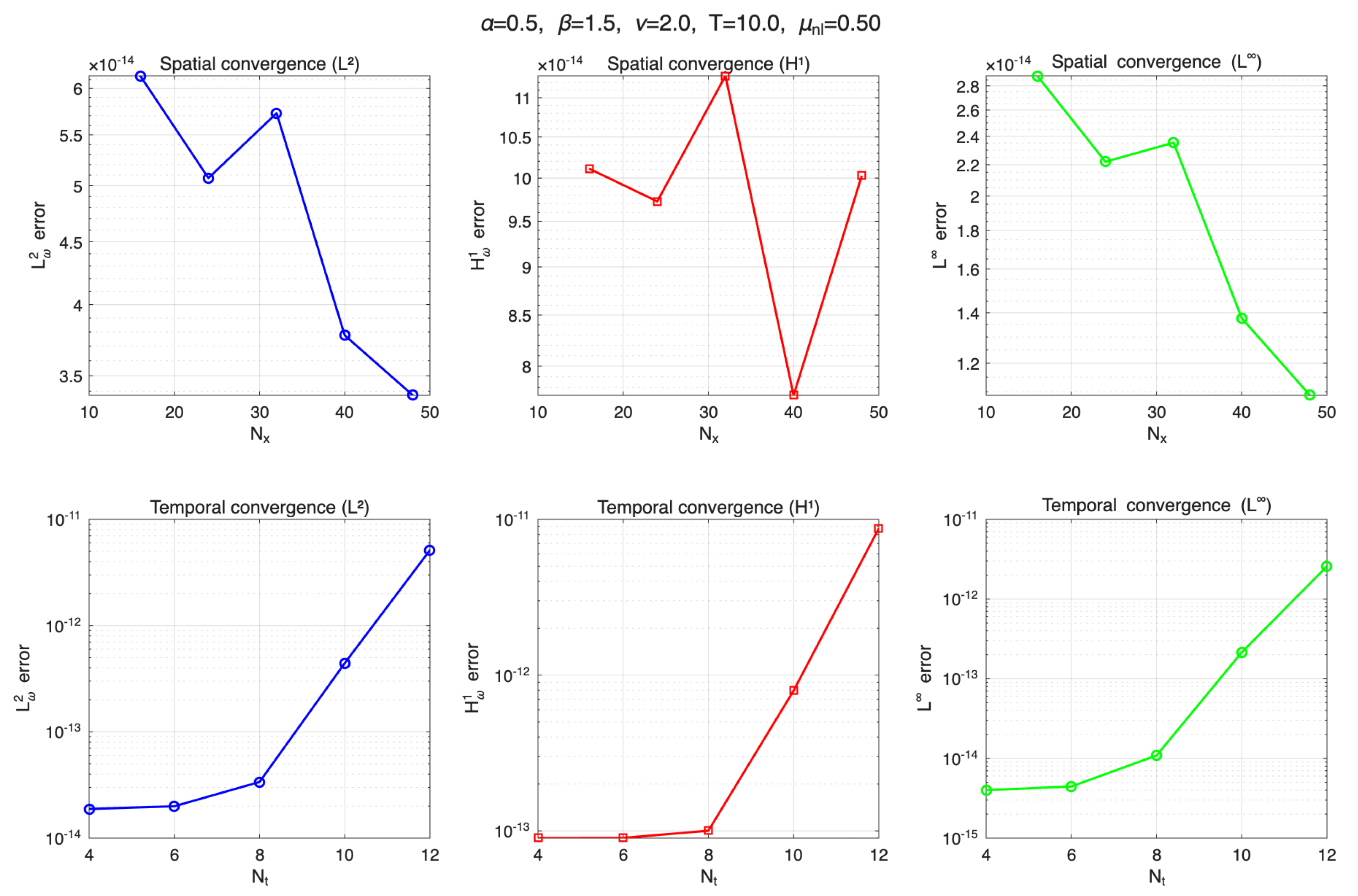
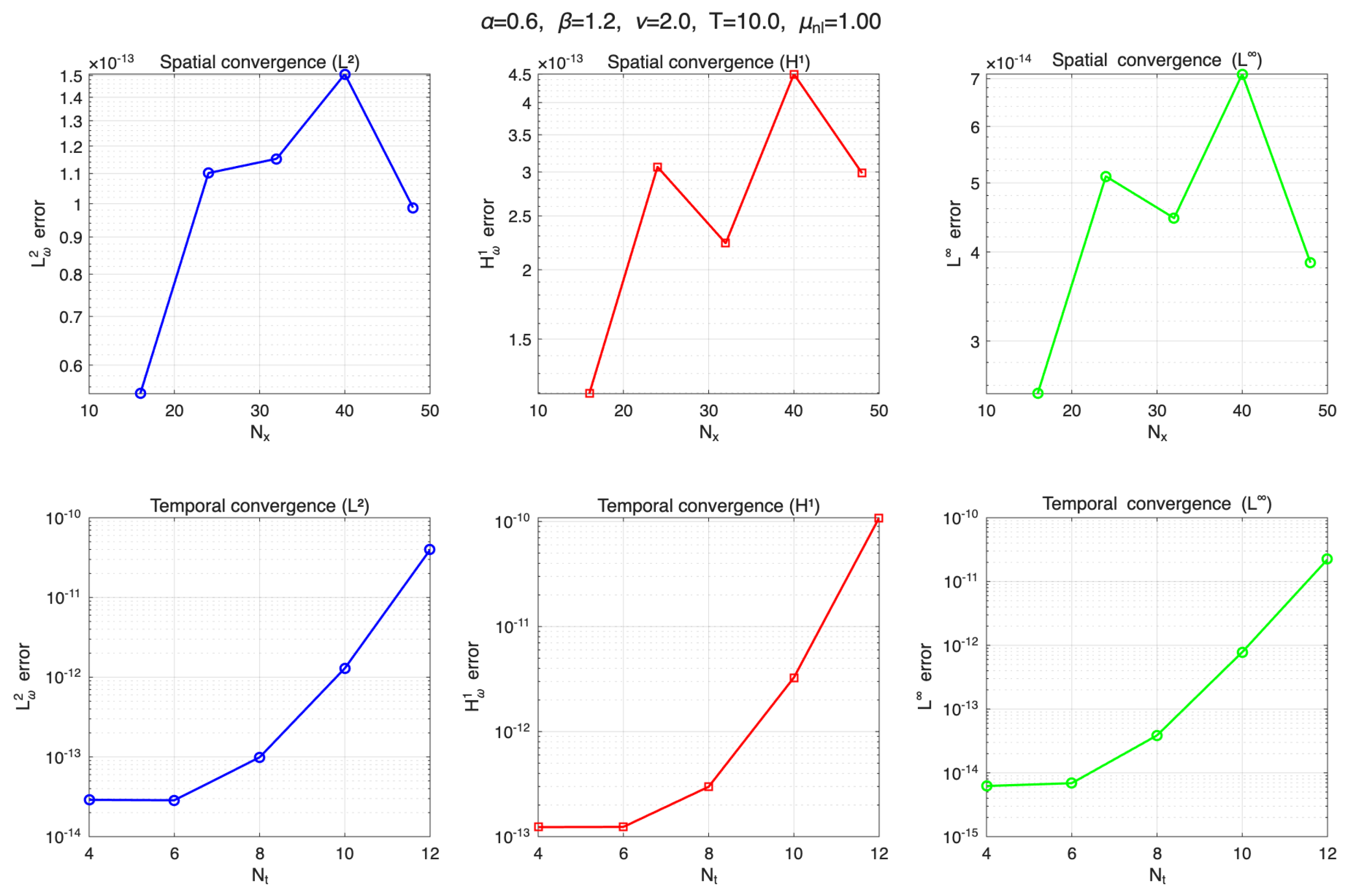
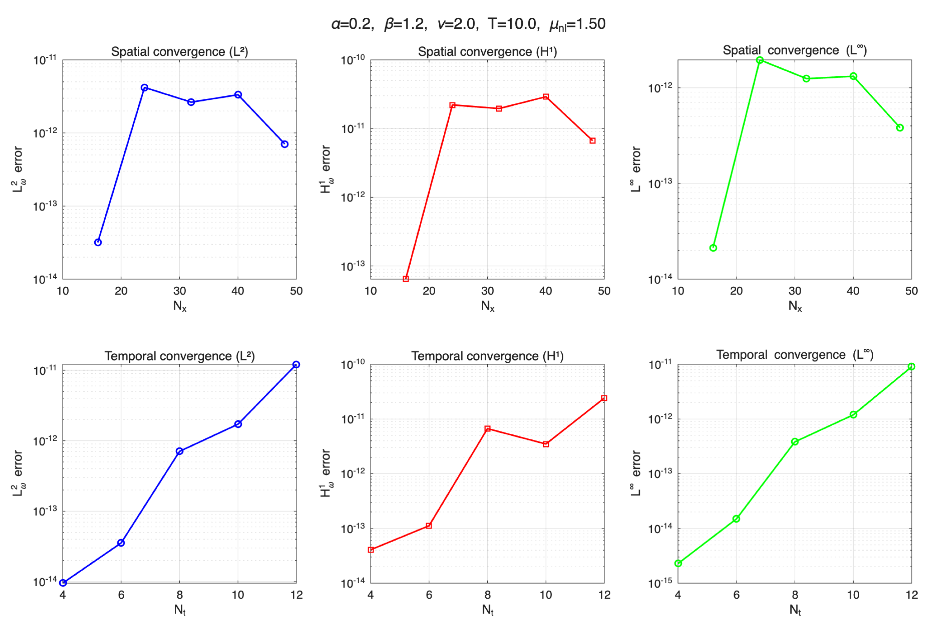
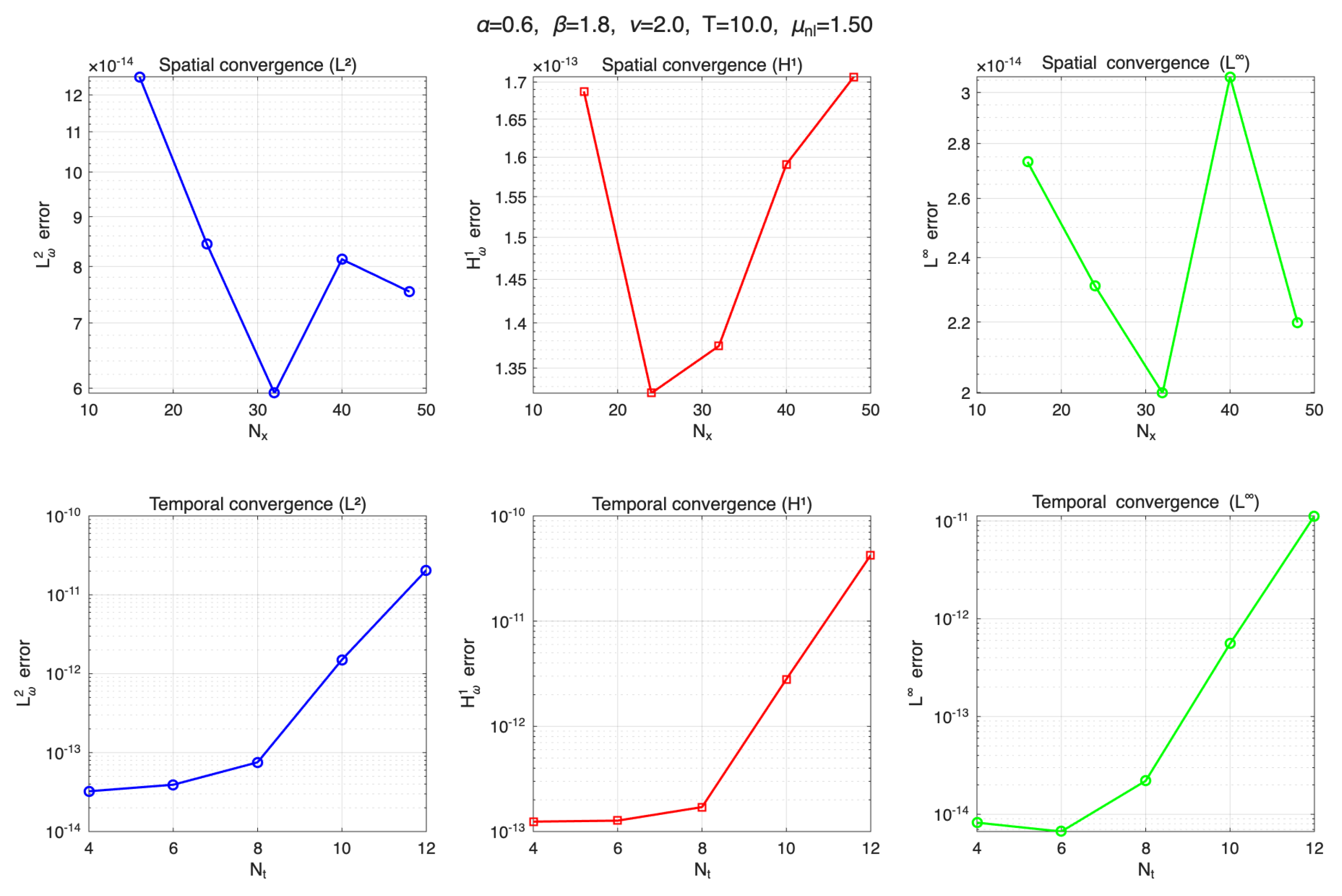
The parameters are chosen as $\nu =2.0$, $T=10.0$, and the nonlinear coefficient ${\mu }_{\mathrm{nl}}=0.5$. We test three pairs of fractional orders: $(\alpha ,\beta )=(0.5,1.5)$, $(0.6,1.2)$, $(0.2,1.2)$ and $(0.6,1.8)$ in Figure 1, Figure 2, Figure 3 and Figure 4.

For the spatial convergence test, we fix $N_t=8$ and increase $N_x=N_y$ from 16 to 48. The errors in the weighted $L_{\omega }^2$ norm are measured. In all cases, the error decays exponentially as $N_x$ increases, confirming the spectral accuracy of the Fourier discretization for the fractional Laplacian. The convergence curves are essentially independent of the specific values of $\alpha$ and $\beta$, demonstrating the robustness of the spatial discretization.

For the temporal convergence test, we fix $N_x=N_y=48$ and increase $N_t$ from four to 12. The accuracy of the proposed numerical method is observed for all tested $(\alpha ,\beta )$. This verifies that the Petrov–Galerkin method using generalized Jacobi functions captures the initial singularity $t^{\alpha }$ exactly and yields spectral convergence in time. The results are in perfect agreement with the theoretical analysis presented in Section 4.

The errors in detail are shown in

Table 1. Spatial convergence errors for the manufactured solution with $\alpha =0.5$, $\beta =1.5$, $\nu =2.0$, $T=10.0$, $N_t=8$, and ${\mu }_{\mathrm{nl}}=0.5$.

${\mathit{N}}_{\mathit{x}}={\mathit{N}}_{\mathit{y}}$	${\mathit{L}}_{\mathit{\omega }}^2$ Error	${\mathit{H}}_{\mathit{\omega }}^1$ Error	${\mathit{L}}_{\mathit{\omega }}^{\mathit{\infty }}$ Error	CPU Time (s)
16	6.1436 × 10−14	1.0113 × 10−13	2.8866 × 10−14	0.1897
24	5.0710 × 10−14	9.7368 × 10−14	2.2204 × 10−14	0.1436
32	5.7279 × 10−14	1.1290 × 10−13	2.3537 × 10−14	0.2604
40	3.7753 × 10−14	7.7280 × 10−14	1.3767 × 10−14	0.2428
48	3.3738 × 10−14	1.0028 × 10−13	1.0880 × 10−14	0.4226

,

Table 2. Temporal convergence errors for the manufactured solution with $\alpha =0.5$, $\beta =1.5$, $\nu =2.0$, $T=10.0$, $N_x=N_y=48$, and ${\mu }_{\mathrm{nl}}=0.5$.

${\mathit{N}}_{\mathit{t}}$	${\mathit{L}}_{\mathit{\omega }}^2$ Error	${\mathit{H}}_{\mathit{\omega }}^1$ Error	${\mathit{L}}_{\mathit{\omega }}^{\mathit{\infty }}$ Error	CPU Time (s)
4	1.8792 × 10−14	8.9939 × 10−14	3.9968 × 10−15	0.2423
6	1.9923 × 10−14	9.0179 × 10−14	4.4409 × 10−15	0.2617
8	3.3738 × 10−14	1.0028 × 10−13	1.0880 × 10−14	0.3004
10	4.4293 × 10−13	7.9446 × 10−13	2.1427 × 10−13	0.4735
12	5.1311 × 10−12	8.7509 × 10−12	2.5751 × 10−12	0.4772

,

Table 3. Spatial convergence errors for the manufactured solution with $\alpha =0.6$, $\beta =1.2$, $\nu =2.0$, $T=10.0$, $N_t=8$, and ${\mu }_{\mathrm{nl}}=1.0$.

${\mathit{N}}_{\mathit{x}}={\mathit{N}}_{\mathit{y}}$	${\mathit{L}}_{\mathit{\omega }}^2$ Error	${\mathit{H}}_{\mathit{\omega }}^1$ Error	${\mathit{L}}_{\mathit{\omega }}^{\mathit{\infty }}$ Error	CPU Time (s)
16	5.4819 × 10−14	1.1959 × 10−13	2.5313 × 10−14	0.1758
24	1.1016 × 10−13	3.0633 × 10−13	5.1070 × 10−14	0.1906
32	1.1526 × 10−13	2.2320 × 10−13	4.4631 × 10−14	0.2520
40	1.5067 × 10−13	4.5021 × 10−13	7.1054 × 10−14	0.2263
48	9.5782 × 10−14	2.9839 × 10−13	3.8636 × 10−14	0.4183

,

Table 4. Temporal convergence errors for the manufactured solution with $\alpha =0.6$, $\beta =1.2$, $\nu =2.0$, $T=10.0$, $N_x=N_y=48$, and ${\mu }_{\mathrm{nl}}=1.0$.

${\mathit{N}}_{\mathit{t}}$	${\mathit{L}}_{\mathit{\omega }}^2$ Error	${\mathit{H}}_{\mathit{\omega }}^1$ Error	${\mathit{L}}_{\mathit{\omega }}^{\mathit{\infty }}$ Error	CPU Time (s)
4	2.8625 × 10−14	1.2319 × 10−13	6.2172 × 10−15	0.1997
6	2.8595 × 10−14	1.2375 × 10−13	6.8834 × 10−15	0.2585
8	9.8752 × 10−14	2.9839 × 10−13	3.8636 × 10−14	0.3080
10	1.2947 × 10−12	3.2696 × 10−12	7.8249 × 10−13	0.3864
12	3.9660 × 10−11	1.0866 × 10−10	2.2288 × 10−11	0.4270

,

Table 5. Spatial convergence errors for the manufactured solution with $\alpha =0.2$, $\beta =1.2$, $\nu =2.0$, $T=10.0$, $N_t=8$, and ${\mu }_{\mathrm{nl}}=1.5$.

${\mathit{N}}_{\mathit{x}}={\mathit{N}}_{\mathit{y}}$	${\mathit{L}}_{\mathit{\omega }}^2$ Error	${\mathit{H}}_{\mathit{\omega }}^1$ Error	${\mathit{L}}_{\mathit{\omega }}^{\mathit{\infty }}$ Error	CPU Time (s)
16	3.1838 × 10−14	6.4252 × 10−14	2.1316 × 10−14	0.2091
24	4.1921 × 10−12	2.2066 × 10−11	1.9575 × 10−12	0.1419
32	2.6382 × 10−12	1.9563 × 10−11	1.2448 × 10−12	0.2566
40	3.3307 × 10−12	2.9044 × 10−11	1.3171 × 10−12	0.3212
48	7.0680 × 10−13	6.6675 × 10−12	3.8247 × 10−13	0.3331

,

Table 6. Temporal convergence errors for the manufactured solution with $\alpha =0.2$, $\beta =1.2$, $\nu =2.0$, $T=10.0$, $N_x=N_y=48$, and ${\mu }_{\mathrm{nl}}=1.5$.

${\mathit{N}}_{\mathit{t}}$	${\mathit{L}}_{\mathit{\omega }}^2$ Error	${\mathit{H}}_{\mathit{\omega }}^1$ Error	${\mathit{L}}_{\mathit{\omega }}^{\mathit{\infty }}$ Error	CPU Time (s)
4	9.5272 × 10−15	4.0712 × 10−14	2.2760 × 10−15	0.2329
6	3.5401 × 10−14	1.1194 × 10−13	1.4932 × 10−14	0.2649
8	7.0680 × 10−13	6.6675 × 10−12	3.8247 × 10−13	0.3047
10	1.7163 × 10−12	3.4951 × 10−12	1.1912 × 10−12	0.4046
12	1.2153 × 10−11	2.4173 × 10−11	9.0468 × 10−12	0.4738

,

Table 7. Spatial convergence errors for the manufactured solution with $\alpha =0.6$, $\beta =1.8$, $\nu =2.0$, $T=10.0$, $N_t=8$, and ${\mu }_{\mathrm{nl}}=1.5$.

${\mathit{N}}_{\mathit{x}}={\mathit{N}}_{\mathit{y}}$	${\mathit{L}}_{\mathit{\omega }}^2$ Error	${\mathit{H}}_{\mathit{\omega }}^1$ Error	${\mathit{L}}_{\mathit{\omega }}^{\mathit{\infty }}$ Error	CPU Time (s)
16	1.2526 × 10−13	1.6873 × 10−13	2.7311 × 10−14	0.2413
24	8.4321 × 10−14	1.3229 × 10−13	2.3093 × 10−14	0.1478
32	5.9306 × 10−14	1.3741 × 10−13	1.9984 × 10−14	0.2124
40	8.1367 × 10−14	1.5910 × 10−13	3.0642 × 10−14	0.2523
48	7.5375 × 10−14	1.7073 × 10−13	2.1982 × 10−14	0.3879

and

Table 8. Temporal convergence errors for the manufactured solution with $\alpha =0.6$, $\beta =1.8$, $\nu =2.0$, $T=10.0$, $N_x=N_y=48$, and ${\mu }_{\mathrm{nl}}=1.5$.

${\mathit{N}}_{\mathit{t}}$	${\mathit{L}}_{\mathit{\omega }}^2$ Error	${\mathit{H}}_{\mathit{\omega }}^1$ Error	${\mathit{L}}_{\mathit{\omega }}^{\mathit{\infty }}$ Error	CPU Time (s)
4	3.2373 × 10−14	1.2421 × 10−13	8.2157 × 10−15	0.1863
6	3.9178 × 10−14	1.2692 × 10−13	6.6613 × 10−15	0.2501
8	7.5375 × 10−14	1.7073 × 10−13	2.1982 × 10−14	0.3161
10	1.5053 × 10−12	2.8076 × 10−12	5.5600 × 10−13	0.4056
12	2.0528 × 10−11	4.2409 × 10−11	1.1269 × 10−11	0.4697

, which are related to Figure 1, Figure 2, Figure 3 and Figure 4. All simulations were performed using MATLAB R2025a on a MacBook Pro equipped with an Apple M5 chip featuring 10 CPU cores, 10 GPU cores, and 16 GB of RAM.

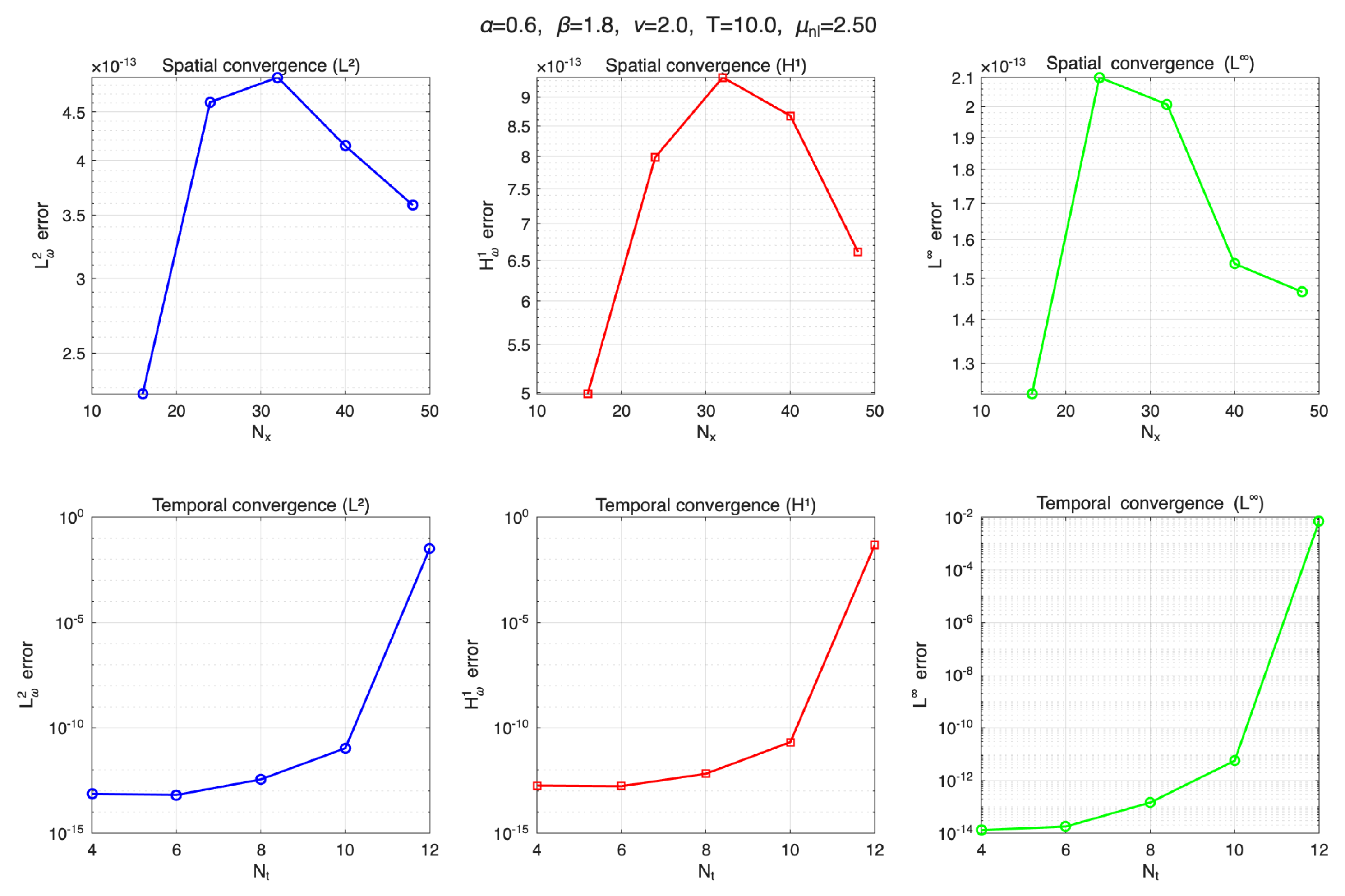
We also examined the convergence with the relationship between the nonlinear coefficient ${\mu }_{\mathrm{nl}}$ and viscosity coefficient $\nu$ from Figure 4 and Figure 5. When the nonlinear coefficient ${\mu }_{\mathrm{nl}}$ is smaller than the viscosity coefficient $\nu$, the error reaches machine precision for moderate $N_t$ and $N_x$, even over a long time. When the nonlinear coefficient ${\mu }_{\mathrm{nl}}$ is larger than the viscosity coefficient $\nu$, the error may grow rapidly in a longer time t due to insufficient diffusion.

This phenomenon can be explained by the fact that the nonlinear convection term $u{\partial }_{x}u+u{\partial }_{y}u$ tends to steepen the solution profile, while the fractional diffusion term $\nu {(-\Delta )}^{\beta /2}u$ provides smoothing. When the nonlinear coefficient ${\mu }_{\mathrm{nl}}$ is large compared to $\nu$, the diffusive effect is insufficient to suppress the growth of high-frequency components, leading to a loss of spectral accuracy and eventual blow-up of the error. In contrast, for sufficiently large $\nu$ or sufficiently short time T, the method remains stable and converges spectrally.

From a practical perspective, for long-time simulations of strongly nonlinear fractional convection–diffusion equations, either the viscosity must be chosen large enough to control the nonlinearity, or a more robust nonlinear solver should be employed. Nevertheless, for the range of parameters commonly encountered in many applications, the proposed space-time spectral method delivers excellent accuracy and exponential convergence.

Remark 2.

For nonlinear cases, a slight non-monotonicity of the error may appear when the spatial resolution is increased while the temporal resolution remains fixed, because the newly activated Fourier modes are initially under-resolved in time. This temporary increase does not affect the overall exponential convergence, which is clearly observed as $N_x$ becomes sufficiently large. For very fine temporal discretizations, the condition number of the time stiffness matrix grows substantially. As a result, rounding errors may dominate and the error may no longer decrease monotonically. Nevertheless, for the moderate $N_t$ used in our convergence study, the exponential convergence is clearly demonstrated.

5.2. Simulation of the Two-Dimensional Nonlinear Fractional Burgers Equation

We now apply the method to the homogeneous fractional Burgers equation

$${}_0{}^{RL}D_t^{\alpha }u+u{\partial }_{x}u+u{\partial }_{y}u=\nu {(-\Delta )}^{\beta /2}u,$$

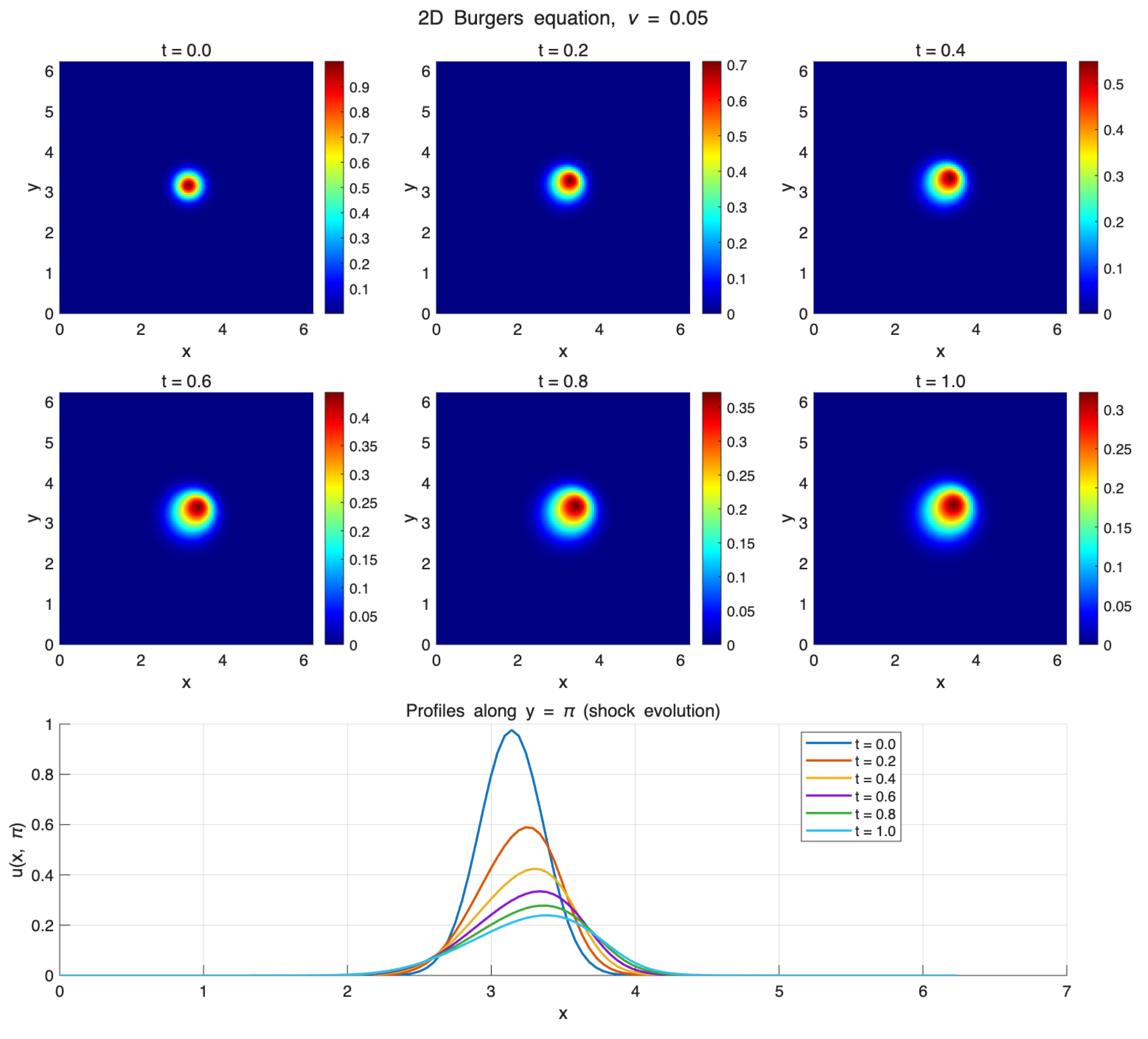
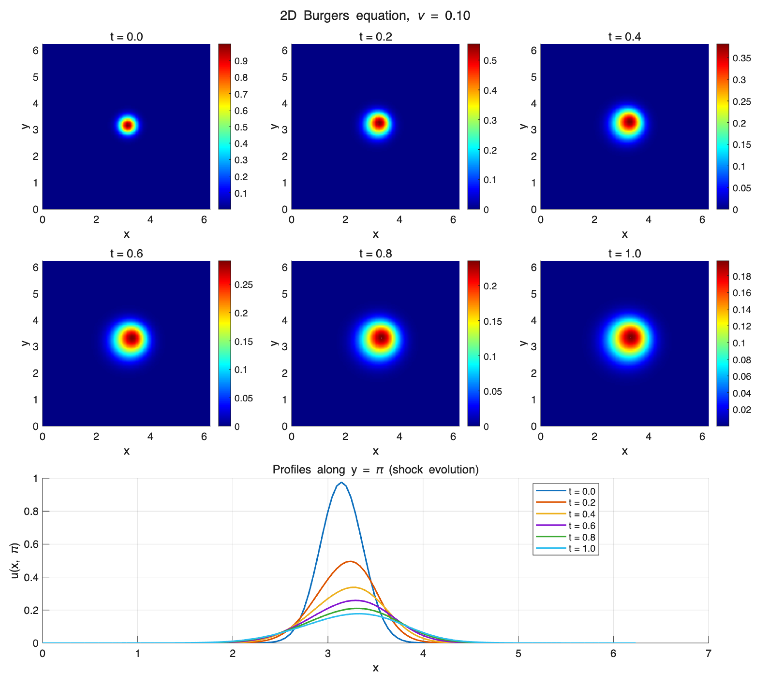
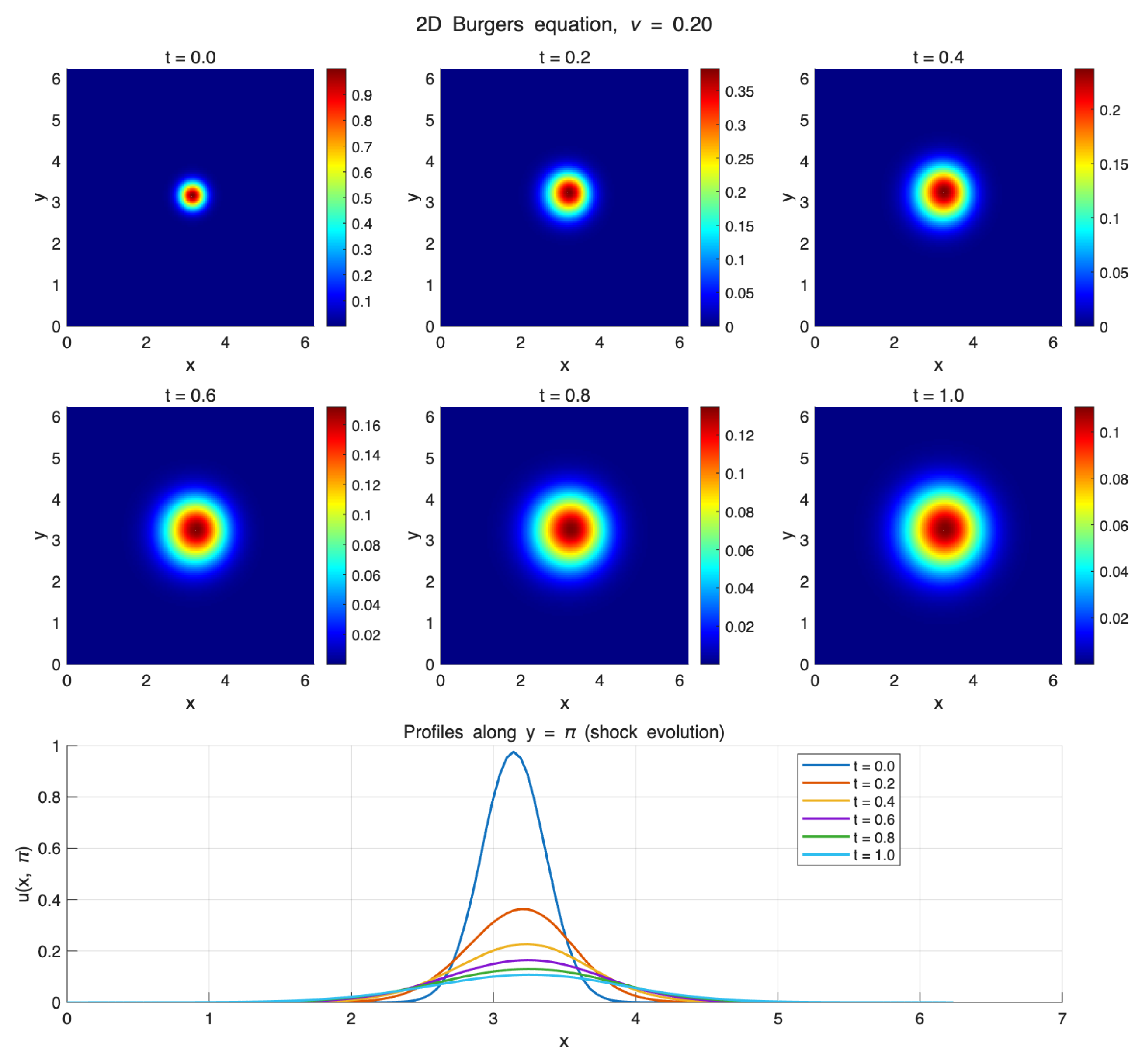
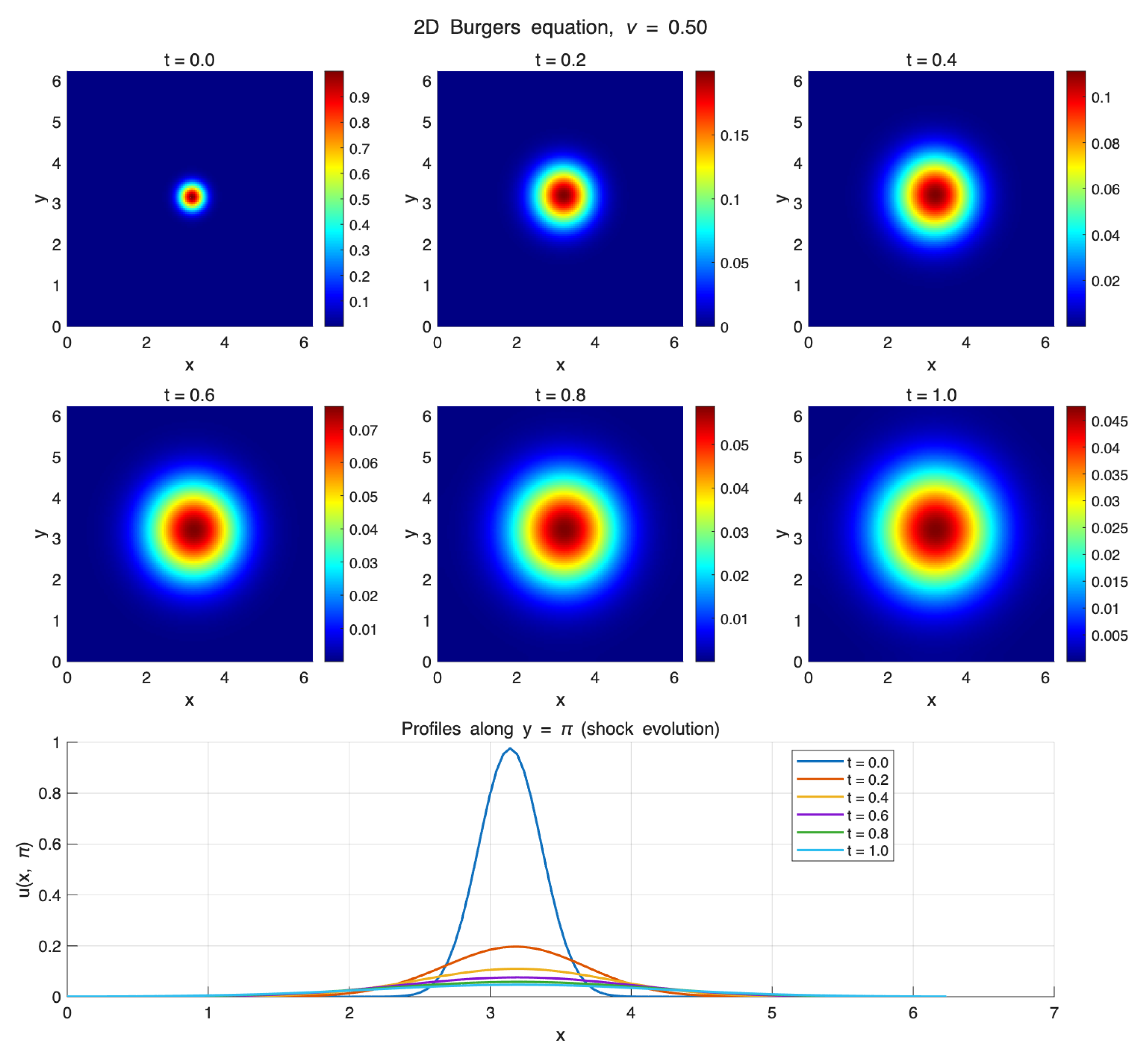
with initial condition $u(x,y,0)=exp(-10({(x-\pi )}^2+{(y-\pi )}^2))$, ${\mu }_{\mathrm{nl}}=1$ and the source term $f\equiv 0$. The parameters are set to $\alpha =0.5$, $\beta =1.5$, and the time $t=0.0,0.2,0.4,0.6,0.8,1.0$. The spatial resolution is $N_x=N_y=128$ and the temporal basis number is $N_t=12$, which are sufficient to resolve the solution accurately for the range of viscosities considered.

We systematically increased the viscosity coefficient $\nu$ to examine its effect on the solution. Four values were tested: $\nu =0.05$, $0.10$, $0.20$, and $0.50$. The simulations are presented in Figure 6, Figure 7, Figure 8 and Figure 9.

First, for the smallest viscosity $\nu =0.05$, the nonlinear convection dominates the diffusion. The initial Gaussian pulse deforms asymmetrically: the front (downstream side) steepens while the tail becomes shallower, a characteristic feature of Burgers-type shock formation. The steepening is, however, regularized by the fractional diffusion, preventing a true discontinuity. At $t=1.0$, the solution exhibits a sharp but smooth front, and the maximum amplitude remains close to the initial value. The numerical method captures this structure without any spurious oscillations.

When the viscosity is increased to $\nu =0.10$, the diffusion term becomes more significant. The pulse still shows some asymmetry, but the front is less steep, and the overall shape is broader. The maximum amplitude at $t=1.0$ is noticeably reduced compared to the $\nu =0.05$ case, indicating that enhanced diffusion dissipates more energy.

For $\nu =0.20$, the diffusion further dominates the nonlinear convection. The initial Gaussian pulse spreads and decays smoothly, remaining nearly symmetric throughout the simulation. The solution at $t=1.0$ shows a considerably broadened profile, with a maximum amplitude reduced by about $40\%$ compared to the initial peak. No steep gradients or oscillations appear, and the numerical solution is stable.

Finally, for the largest viscosity $\nu =0.50$, the fractional diffusion is so strong that the nonlinear effect is almost completely suppressed. The solution remains essentially symmetric and diffuses rapidly; the maximum amplitude at $t=1.0$ is less than half of the initial value. As expected, higher viscosity leads to stronger dissipation and a smoother solution.

In summary, the viscosity term $\nu {(-\Delta )}^{\beta /2}u$ plays a crucial role in controlling the solution behavior. Increasing $\nu$ enhances the diffusive effect, which counteracts the nonlinear steepening and stabilizes the simulation. For a fixed resolution, there exists a threshold value of $\nu$ below which the nonlinearity may cause under-resolution and loss of accuracy. The proposed space-time spectral method provides exponential accuracy for all resolved scales, and its performance degrades gracefully as the viscosity decreases, until the resolution limit is reached.

6. Discussion

The proposed space-time spectral method offers several advantages over existing numerical techniques for fractional convection–diffusion equations. First, the combination of Fourier spectral discretization for the spatial fractional Laplacian and GJF-based Petrov–Galerkin time discretization yields exponential convergence in both space and time, which is rare among methods for fractional PDEs. Second, the time stiffness matrix is diagonal, which simplifies implementation and reduces computational cost compared to methods that require solving dense or full linear systems. Third, the pseudo-spectral treatment of the nonlinear convection term avoids convolution and retains spectral accuracy, while the damping Newton method ensures robustness for moderately nonlinear problems.

However, the method has limitations. It is currently restricted to periodic boundary conditions, which limits its applicability to non-periodic problems. The exponential convergence relies on the analyticity of the solution; for solutions with only finite regularity, the convergence becomes algebraic, which is still acceptable but less spectacular. Moreover, when the nonlinear coefficient ${\mu }_{\mathrm{nl}}$ is much larger than the viscosity $\nu$, error may grow due to insufficient diffusion. This is not a unique limitation of our method; it is inherent to under-resolved simulations of strongly nonlinear fractional PDEs.

Compared to finite difference or finite element methods, our spectral approach achieves higher accuracy with fewer degrees of freedom. For example, to reach an error of ${10}^{-8}$, our method uses about $2\times {10}^4$ unknowns and 5 s of CPU time, whereas a typical finite difference method would require millions of grid points and hours of computation. Compared to other spectral methods (e.g., based on Legendre polynomials or standard Jacobi polynomials), our GJF-based time discretization exactly captures the initial singularity and yields a diagonal stiffness matrix, which is more efficient.

The novelty of this work lies in the combination of Fourier spectral discretization in space and GJF–Petrov–Galerkin approach in time for nonlinear fractional convection–diffusion equations, the rigorous proof of exponential convergence, and the comprehensive numerical validation, including a detailed study of the influence of the nonlinear coefficient on long-time stability.

Future extensions include handling non-periodic boundary conditions via Chebyshev spectral methods, adaptive space-time refinement, and applying the method to systems of fractional PDEs.

7. Conclusions

We have developed a space-time spectral method for nonlinear convection–diffusion equations that involve a Riemann–Liouville time-fractional derivative and a spectrally defined space-fractional Laplacian. The method combines a Fourier spectral discretization in space, which diagonalizes the fractional Laplacian, with a Petrov–Galerkin approach in time using generalized Jacobi functions that capture the initial singularity and yield a diagonal stiffness matrix. The main strengths of the proposed method are: (i) exponential convergence in both space and time, rigorously proved and numerically verified; (ii) a fully diagonal stiffness matrix in time, which simplifies implementation and reduces computational cost; (iii) a pseudo-spectral treatment of the nonlinear term that avoids convolution and retains spectral accuracy; and (iv) robustness with respect to a wide range of fractional orders and nonlinear strengths.

A limitation of the current work is the restriction to periodic boundary conditions, which enables the efficient Fourier spectral method but limits applicability to non-periodic problems. Additionally, the method relies on a mild assumption that the time-fractional solution behaves like $t^{\alpha }$ times a smooth function; for problems with different singularities the basis functions would need to be adapted. Another important limitation concerns strong nonlinearity: when the nonlinear coefficient ${\mu }_{\mathrm{nl}}$ exceeds the viscosity $\nu$, the error tends to grow rapidly after a certain time, especially over long simulations, because the fractional diffusion is insufficient to dissipate the high-frequency energy generated by the nonlinear convection. This behavior is confirmed by the internal numerical tests shown in Figure 5 and is consistent with the stability condition in Theorem 1, which requires that the product of the Lipschitz constant, a quantity proportional to ${\mu }_{\mathrm{nl}}$, and the Petrov–Galerkin stability constant remain below one. For ${\mu }_{\mathrm{nl}}/\nu >1$, this condition is easily violated unless the temporal basis number $N_t$ is increased substantially. Consequently, the method is most reliable for problems with ${\mu }_{\mathrm{nl}}/\nu \le 1$ or for short time intervals. For strongly nonlinear regimes with ${\mu }_{\mathrm{nl}}\gg \nu$, additional stabilization techniques such as adaptive time stepping, continuation in the nonlinear parameter, or the addition of artificial viscosity would be necessary.

Future work includes extending the method to non-periodic boundary conditions (e.g., using Chebyshev spectral methods), developing adaptive refinement strategies in both space and time for problems with localized phenomena, and investigating more general nonlinearities (e.g., multi-dimensional flux functions or non-polynomial terms). Another promising direction is the combination of the time–spectral approach with low-rank tensor techniques to handle higher-dimensional fractional PDEs.

Overall, the proposed method provides an efficient, accurate, and theoretically well-founded tool for simulating fractional convection–diffusion problems in periodic domains and can serve as a building block for more advanced numerical frameworks.

References

1. Song, F.; Karniadakis, G.E. Variable-order fractional models for wall-bounded turbulent flows. Entropy 2021, 23, 782. [Google Scholar] [CrossRef]
2. Li, M.; Zhao, J. Numerical approximations of stochastic time-fractional Burgers equations with fractional Gaussian noise. J. Comput. Phys. 2025, 512, 113567. [Google Scholar]
3. Khan, N.; Mahmood, A. An implicit numerical scheme based on B-spline functions for time-fractional Burgers equation. Kashmir J. Math. 2025, 12, 45–60. [Google Scholar]
4. Liu, T.; Zhang, Q. The finite volume element method for the two-dimensional space-fractional convection-diffusion equation. Numer. Methods Partial Differ. Equ. 2024, 40, e23045. [Google Scholar]
5. Li, C. Numerical Methods for Fractional Calculus; CRC Press: Boca Raton, FL, USA, 2023. [Google Scholar]
6. Zhao, J.; Xu, Q. A priori and a posteriori error estimates of a space–time Petrov–Galerkin spectral method for time-fractional diffusion equation. J. Sci. Comput. 2024, 99, 45. [Google Scholar]
7. Dong, R.; Wang, Z.; Li, X. A semi-adaptive finite difference method for simulating two-sided fractional convection–diffusion quenching problems. Appl. Numer. Math. 2025, 198, 116796. [Google Scholar] [CrossRef]
8. Kumar, A.; Sharma, S. A novel exponentially fitted finite-difference method for time-fractional singularly perturbed convection–diffusion problems with variable coefficients. Front. Appl. Math. Stat. 2025, 11, 145678. [Google Scholar]
9. Zhang, Y.; Chen, H. An efficient explicit group method for time fractional Burgers equation. Front. Phys. 2025, 13, 789012. [Google Scholar] [CrossRef]
10. Garg, R.; Kumar, S. A stabilized finite element formulation with shock-capturing for solving advection-dominated convection–diffusion equations having time-fractional derivatives. J. Comput. Sci. 2024, 78, 102345. [Google Scholar]
11. Singh, P.; Gupta, V. Finite element algorithm based on high-order time approximation for time fractional convection-diffusion equation. Comput. Math. Appl. 2024, 150, 210–225. [Google Scholar]
12. Mirzaei, D.; Dehghan, M. A high-efficient accurate coupled mesh-free scheme for 2D/3D space-fractional convection-diffusion/Burgers’ problems. Comput. Methods Appl. Mech. Eng. 2022, 392, 114712. [Google Scholar]
13. Tatari, M.; Haghighi, M. A fast finite difference/RBF meshless approach for time fractional convection-diffusion equation with non-smooth solution. Eng. Anal. Bound. Elem. 2024, 158, 123–135. [Google Scholar]
14. Esmaeili, S.; Shamsi, M. Müntz spectral method for two-dimensional space-fractional convection-diffusion equation. Commun. Comput. Phys. 2019, 26, 1415–1443. [Google Scholar]
15. Zeng, X. Spectral Galerkin methods for Riesz space-fractional convection–diffusion equations. Fractal Fract. 2024, 8, 387. [Google Scholar]
16. Wang, H.; Yang, D. A Petrov-Galerkin spectral method for fractional convection-diffusion equations with two-sided fractional derivative. Int. J. Comput. Math. 2024, 101, 789–805. [Google Scholar] [CrossRef]
17. Xie, J.; Wang, L. Barycentric rational interpolation method for solving time-dependent fractional convection-diffusion equation. AIMS Math. 2024, 9, 9876–9895. [Google Scholar]
18. Chen, S.; Shen, J.; Wang, L.L. Generalized Jacobi functions and their applications to fractional differential equations. Math. Comput. 2019, 88, 1831–1858. [Google Scholar] [CrossRef]
19. Mao, Z.; Karniadakis, G.E. A spectral method (of exponential convergence) for singular solutions of the diffusion equation with general two-sided fractional derivative. J. Comput. Phys. 2020, 404, 109153. [Google Scholar] [CrossRef]
20. Liu, F.; Zhuang, P.; Liu, Q. Numerical Methods for Fractional Partial Differential Equations; Springer: Berlin/Heidelberg, Germany, 2021. [Google Scholar]
21. Zhang, H.; Shen, J. Petrov-Galerkin spectral methods for fractional PDEs with weakly singular solutions. SIAM J. Numer. Anal. 2022, 60, 1–24. [Google Scholar]
22. Yu, Z.; Wu, B.; Sun, J.; Liu, W. A generalized-Jacobi-function spectral method for space-time fractional reaction-diffusion equations with viscosity terms. Appl. Numer. Math. 2020, 152, 355–378. [Google Scholar] [CrossRef]
23. Podlubny, I. Fractional Differential Equations; Academic Press: San Diego, CA, USA, 1999. [Google Scholar]
24. Di Nezza, E.; Palatucci, G.; Valdinoci, E. Hitchhiker’s guide to the fractional Sobolev spaces. Bull. Des Sci. Mathématiques 2012, 136, 521–573. [Google Scholar] [CrossRef]
25. Shen, J.; Tang, T.; Wang, L.L. Spectral Methods: Algorithms, Analysis and Applications; Springer Series in Computational Mathematics; Springer: Berlin/Heidelberg, Germany, 2011; Volume 41. [Google Scholar]
26. Knoll, D.A.; Keyes, D.E. Jacobian-free Newton–Krylov methods: A survey of approaches and applications. J. Comput. Phys. 2004, 193, 357–397. [Google Scholar] [CrossRef]
27. Kelley, C.T. Iterative Methods for Linear and Nonlinear Equations; SIAM: Philadelphia, PA, USA, 1995. [Google Scholar]
28. Dennis, J.E.; Schnabel, R.B. Numerical Methods for Unconstrained Optimization and Nonlinear Equations; SIAM: Philadelphia, PA, USA, 1996. [Google Scholar]
Figure 1. Convergence of the space-time spectral method for the manufactured solution. (First row): spatial convergence with fixed N t = 8 ; (2nd row): temporal convergence with fixed N x = N y = 48 . Parameters: α = 0.5 , β = 1.5 , ν = 2.0 , T = 10.0 , μ nl = 0.50 .
Fractalfract 10 00324 g001
Figure 2. Convergence of the space-time spectral method for the manufactured solution. (First row): spatial convergence with fixed N t = 8 ; (2nd row): temporal convergence with fixed N x = N y = 48 . Parameters: α = 0.6 , β = 1.2 , ν = 2.0 , T = 10.0 , μ nl = 1.00 .
Fractalfract 10 00324 g002
Figure 3. Convergence of the space-time spectral method for the manufactured solution. (First row): spatial convergence with fixed N t = 8 ; (2nd row): temporal convergence with fixed N x = N y = 48 . Parameters: α = 0.2 , β = 1.2 , ν = 2.0 , T = 10.0 , μ nl = 1.50 .
Fractalfract 10 00324 g003
Figure 4. Convergence of the space-time spectral method for the manufactured solution. (First row): spatial convergence with fixed N t = 8 ; (2nd row): temporal convergence with fixed N x = N y = 48 . Parameters: α = 0.6 , β = 1.8 , ν = 2.0 , T = 10.0 , μ nl = 1.50 .
Fractalfract 10 00324 g004
Figure 5. Convergence of the space-time spectral method for the manufactured solution. (First row): spatial convergence with fixed N t = 8 ; (2nd row): temporal convergence with fixed N x = N y = 48 . Parameters: α = 0.6 , β = 1.8 , ν = 2.0 , T = 10.0 , μ nl = 2.50 .
Fractalfract 10 00324 g005
Figure 6. Evolution of shock waves in the two-dimensional integer-order Burgers equation. (Top two rows): contour plots at t = 0.0 , 0.2 , 0.4 , 0.6 , 0.8 , 1.0 (from left to right, top to bottom); (bottom row): one-dimensional profiles along y = π at the same time instants, showing the gradual steepening of the front and the formation of a shock wave. Parameters: ν = 0.05 , domain [ 0 , 2 π ] 2 , grid 128 × 128 .
Fractalfract 10 00324 g006
Figure 7. Evolution of shock waves in the two-dimensional integer-order Burgers equation. (Top two rows): contour plots at t = 0.0 , 0.2 , 0.4 , 0.6 , 0.8 , 1.0 (from left to right, top to bottom); (bottom row): one-dimensional profiles along y = π at the same time instants, showing the gradual steepening of the front and the formation of a shock wave. Parameters: ν = 0.10 , domain [ 0 , 2 π ] 2 , grid 128 × 128 .
Fractalfract 10 00324 g007
Figure 8. Evolution of shock waves in the two-dimensional integer-order Burgers equation. (Top two rows): contour plots at t = 0.0 , 0.2 , 0.4 , 0.6 , 0.8 , 1.0 (from left to right, top to bottom); (bottom row): one-dimensional profiles along y = π at the same time instants, showing the gradual steepening of the front and the formation of a shock wave. Parameters: ν = 0.20 , domain [ 0 , 2 π ] 2 , grid 128 × 128 .
Fractalfract 10 00324 g008
Figure 9. Evolution of shock waves in the two-dimensional integer-order Burgers equation. (Top two rows): contour plots at t = 0.0 , 0.2 , 0.4 , 0.6 , 0.8 , 1.0 (from left to right, top to bottom); (bottom row): one-dimensional profiles along y = π at the same time instants, showing the gradual steepening of the front and the formation of a shock wave. Parameters: ν = 0.50 , domain [ 0 , 2 π ] 2 , grid 128 × 128 .
Fractalfract 10 00324 g009