Iterative Generation and Generalized Degree Distribution of Higher-Order Fractal Scale-Free Networks

Abstract

Fractals represent one of the fundamental manifestations of complexity, and fractal networks serve as tools for characterizing and investigating the fractal structures and properties of large-scale systems. Higher-order networks have emerged as a research hotspot due to their ability to express interactions among multiple nodes. This study proposes an iterative generation model for higher-order fractal networks. The iteration is controlled by three parameters: the dimension $K$ of the simplicial complex, the multiplier $m$, and the iteration count $t$. The constructed network is a pure simplicial complex. Theoretical analysis using the similarity dimension and experimental verification using the box-counting dimension demonstrate that the generated networks exhibit fractal characteristics. When the multiplier $m$ is large, the generalized degree distribution of the generated networks exhibits scale-free properties.

1. Introduction

Fractal theory provides a powerful framework for characterizing fragmented and complex phenomena in nature. Within complex networks, many exhibit fractal characteristics, including hyperlinks on the World Wide Web [1], genetic regulatory networks of S. cerevisiae and E. coli studied by Yook et al. [2], and co-occurrence networks of keyword terms in internet comment texts [3]. The prevalence of this fractal structure is not coincidental. It has been demonstrated that fractal features confer functional advantages on networks, including enhanced robustness against static and dynamic targeted attacks on nodes and links [4], and greater flexibility in choosing microchannel dimensions to achieve uniform flow distribution [5].

A deep understanding of network structures also requires characterizing interaction patterns. Many collective behaviors observed in real-world systems arise from group interaction, such as competition and cooperation in ecosystems [6,7], higher-order topological structures in the brain connectome [8], hub coordination dynamics in transportation systems [9], and the early growth of semantic feature networks in cognitive systems [10]. These collective phenomena extend beyond traditional descriptions based on pairwise connections. Consequently, higher-order networks, which capture relationships beyond pairwise interactions, are gaining increasing attention. Concurrently, researchers have observed that certain real-world networks exhibit both higher-order organization and fractal characteristics. Examples include partial phase synchronization on simplicial complexes around a brain hub [11] and information dissemination on social hypernetworks [12]. It is noteworthy that if we re-examine many systems previously shown to possess both fractal and scale-free properties, such as protein–protein interaction networks [13,14], airport networks studied by Guo et al. [15], from a higher-order structural perspective, we find that these systems also involve complex collective interactions.

However, the integration of fractal characteristics and higher-order structures into a unified network generation model remains underexplored. This gap arises because classical fractal network generation models, such as the Song–Havlin–Makse (SHM) model [16] and the ($u$, $v$)-flower [17], operate on pairwise interactions. By contrast, higher-order network models focus on reproducing, explaining, and predicting higher-order interactions in complex systems [18], and they devote limited attention to generating fractal features. This divergence in the basic unit of operation and the core design goals creates a theoretical gap: a general generative framework capable of producing both fractal and higher-order structures is currently lacking.

To address this challenge, this study aims to develop an iterative generative model for higher-order fractal scale-free networks. We define an iterative algorithm whose behavior is determined by a triple of parameters $(K,m,t)$, representing the dimension of the simplicial complex, the multiplier, and the iteration count, respectively. The generated network is a pure $K$-dimensional simplicial complex. Its fractal dimension is controllable. When the parameter $m$ is large, the network’s generalized degree distribution exhibits scale-free properties.

2. Related Work

2.1. Higher-Order Networks

A higher-order network is capable of characterizing interactions among multiple nodes. One type comprises higher-order networks formed by hypernodes and hyperedges, while another consists of a simplicial complex formed by simplices and their faces [19]. A hypergraph consists of a set of nodes and a set of hyperedges, which specify which nodes participate in interactions and in what manner [18]. Hypergraphs provide the most general and unconstrained description of higher-order interactions. In contrast, a simplicial complex can be viewed as a hypergraph with an additional requirement called downward closure, which states that if an interaction exists among a set of entities, every possible sub-interaction also exists [19].

Higher-order network models can be classified into equilibrium and non-equilibrium models based on the type of stochastic process they employ. Equilibrium models are defined as static distributions over higher-order systems, treating the system as static and drawn from a fixed distribution. In contrast, the vast majority of non-equilibrium models focus on continuously growing systems [18]. Because the model proposed in this paper evolves as the iteration count increases, it conceptually belongs to the paradigm of non-equilibrium models. Therefore, we focus on the construction methods and characteristics of existing non-equilibrium models.

Among non-equilibrium hypergraph models, the evolving hypernetwork model proposed by Wang et al. is a canonical example [20]. This model incorporates two evolutionary mechanisms: hyperedge growth and hyperedge preferential attachment, which together define the dynamics of a growing hypernetwork. Subsequent variants have enhanced the realism of such models by introducing mechanisms for variable hyperedge sizes [21] and diverse strategies for selecting existing nodes to join new hyperedges [22]. These models are generally designed to reproduce characteristic features observed in empirical systems. For non-equilibrium models of simplicial complexes, a significant branch is the Network Geometry with Flavor (NGF) model [23]. The NGF model achieves growth by attaching new $d$-dimensional simplices to existing $(d-1)$-dimensional faces with a probability that depends on the face’s energy and its current number of attachments. Another class of methods generates a sequence of simplicial complexes by transforming a growing sequence of graphs (with ordered node additions) into their clique complexes, i.e., by treating each complete subgraph (clique) as a simplex [10].

2.2. Fractal Networks and Pseudofractal Networks

In network modeling, both fractal networks and pseudo-fractal networks are generated through iterative rules and exhibit a visual hierarchical structure, yet their nature and properties differ fundamentally. The core characteristic of fractal networks is their measurable scale invariance, typically reflected in a finite fractal dimension [16]. This property implies that fractal networks lack small-world properties [24]. In contrast, pseudo-fractal networks do not possess a finite fractal dimension and often exhibit small-world characteristics [17].

The modeling of fractal and pseudo-fractal networks has taken two primary paths. The first path is exemplified by the SHM model [16], in which a probabilistic parameter governs the addition of shortcuts between boxes during the inverse renormalization growth process. Within a unified framework, this mechanism enables continuous tuning between fractal scaling and small-world properties. The second path relies on completely deterministic iterative generators. A prominent example is the ($u$, $v$)-flower model [17], constructed recursively by replacing each edge in generation $n$ with two parallel paths of lengths $u$ and $v$ (where $u\le v$). For $u>1$, the network is fractal with finite dimension; for $u=1$, it becomes a small-world (infinite-dimensional) transfractal. The well-known pseudo-fractal scale-free web of Dorogovtsev et al. [25] is exactly the (1, 2)-flower. Ma and Wang [26] proposed a growing fractal tree network constructed by recursively replacing each edge with a fixed pattern of new vertices and attached leaves, which yields a deterministic fractal structure. Whether fractal or pseudo-fractal, the fundamental unit of interaction in all the aforementioned networks is the pairwise interaction. This constraint forces complex group interactions to be projected onto binary networks, thereby losing essential higher-order information. Therefore, it is necessary to explore fractal structures within a framework of higher-order interactions.

2.3. Higher-Order Fractal Networks

Research on modeling higher-order fractal networks follows two primary perspectives. One concerns the mathematical representation of interactions, namely, hypergraphs versus simplicial complexes. The other concerns the resulting geometric property of the network, namely, fractal versus pseudo-fractal. Vallée et al. [27] proposed the fractal hypergraph model and presented a formal semantics of SystemC components based on fractal hypergraphs. Berec [28] established an essential connection between the Lyapunov exponents and the $d$-regular hypergraph fractal set. Ma et al. [29] constructed a fractal hypernetwork model, which is named $2k$ uniform (1, 3) flower hypernetwork. Zheng et al. [30] demonstrated unconventional higher-order topological phenomena in fractal lattices with a Sierpiński acoustic metamaterial. Xie et al. [31] constructed pseudo-fractal simplicial complexes and investigated their combinatorial properties. Shang [32] proposes a generative model that yields higher-order networks with scale-free and small-world properties, and analytically studied properties such as clique distribution and the Sombor index. Although that study did not discuss the fractal characteristics, its small-world structure belongs to the pseudo-fractal networks as defined in Section 2.2. However, these models generally lack adequate control over the fractal dimension. They generate either pseudo-fractal networks or, when the hyperedge size or simplicial complex dimension is fixed, yield a fractal dimension that is constant and non-tunable. These limitations restrict the ability of such networks to model complex systems and their functional tunability. Therefore, it is crucial to construct a general higher-order fractal network model that can overcome the aforementioned constraints.

3. Preliminaries and Model Setup

This section presents the fundamental concepts of higher-order networks and the model construction.

3.1. Fundamental Concepts of Higher-Order Networks

3.1.1. Simplicial Complexes and Their Dimensions

A set $\alpha =[v_0,v_1,v_2,\dots ,v_K]$ comprising $K+1$ interacting nodes is termed a $K$-dimensional simplex $\alpha$, denoted as a $K$-simplex $\alpha$. For example, a 0-simplex is a point, a 1-simplex is an edge, a 2-simplex is a triangle, a 3-simplex is a tetrahedron, and so on. A face of a $K$-simplex $\alpha$ is a simplex $\beta$ formed by a proper subset of the simplex. For instance, the faces of a 3-simplex (tetrahedron) are four 0-simplices (nodes), six 1-simplices (edges) and four 2-simplices (triangles). The simplicial complex $\mathcal{K}$ is the set of simplices closed under inclusion of faces in each simplex, i.e., if $\alpha \in \mathcal{K}$ and $\beta \subset \alpha$, then $\beta \in \mathcal{K}$. The dimension $K$ of a simplicial complex is the maximum dimension of its simplices. In particular, a simplicial complex consisting of a set of $K$-simplices and their faces is a pure $K$-dimensional simplicial complex [19,33].

3.1.2. Network Skeleton

The $n$-skeleton of a $K$-dimensional simplicial complex $\mathcal{K}$ consists of all simplices of dimension at most $n$ [34]. Specifically, a 0-skeleton is the vertex set, while a 1-skeleton is denoted as $\mathcal{G}=\left\{\mathcal{V},\mathcal{E}\right\}$, where $\mathcal{V}$ and $\mathcal{E}$ represent the vertex set and edge set of $\mathcal{G}$, respectively.

3.1.3. Generalized Degree and Generalized Degree Distribution

When studying network properties, researchers often focus on the degree distribution, as it significantly influences global dynamics. The concepts of degree and degree distribution extend naturally to simplicial complexes, where they are termed the generalized degree and the generalized degree distribution, respectively [23,35].

The generalized degree $k_{K,L}\left(\beta \right)$ denotes the number of $K$-simplices associated with an $L$-simplex $\beta$. When $K>L$, it denotes the number of $K$-simplices contained within the $L$-simplex $\beta$; when $K<L$, it denotes the number of $K$-dimensional faces within the $L$-simplex $\beta$, where $k_{K,L}=\left(\begin{array}{c}L+1\\ K+1\end{array}\right)$. In this paper, the probability $P_{K,L}\left(k\right)$ that any $L$-simplex in a pure $K$ dimensional simplicial complex $\mathcal{K}$ has a generalized degree of $k=k_{K,L}$ is defined as the $L$-dimensional generalized degree distribution of $\mathcal{K}$, where $L=0,1,2,\dots ,K-1$. Subsequent sections shall investigate the generalized degree distributions of each dimension for the constructed network.

3.2. Model

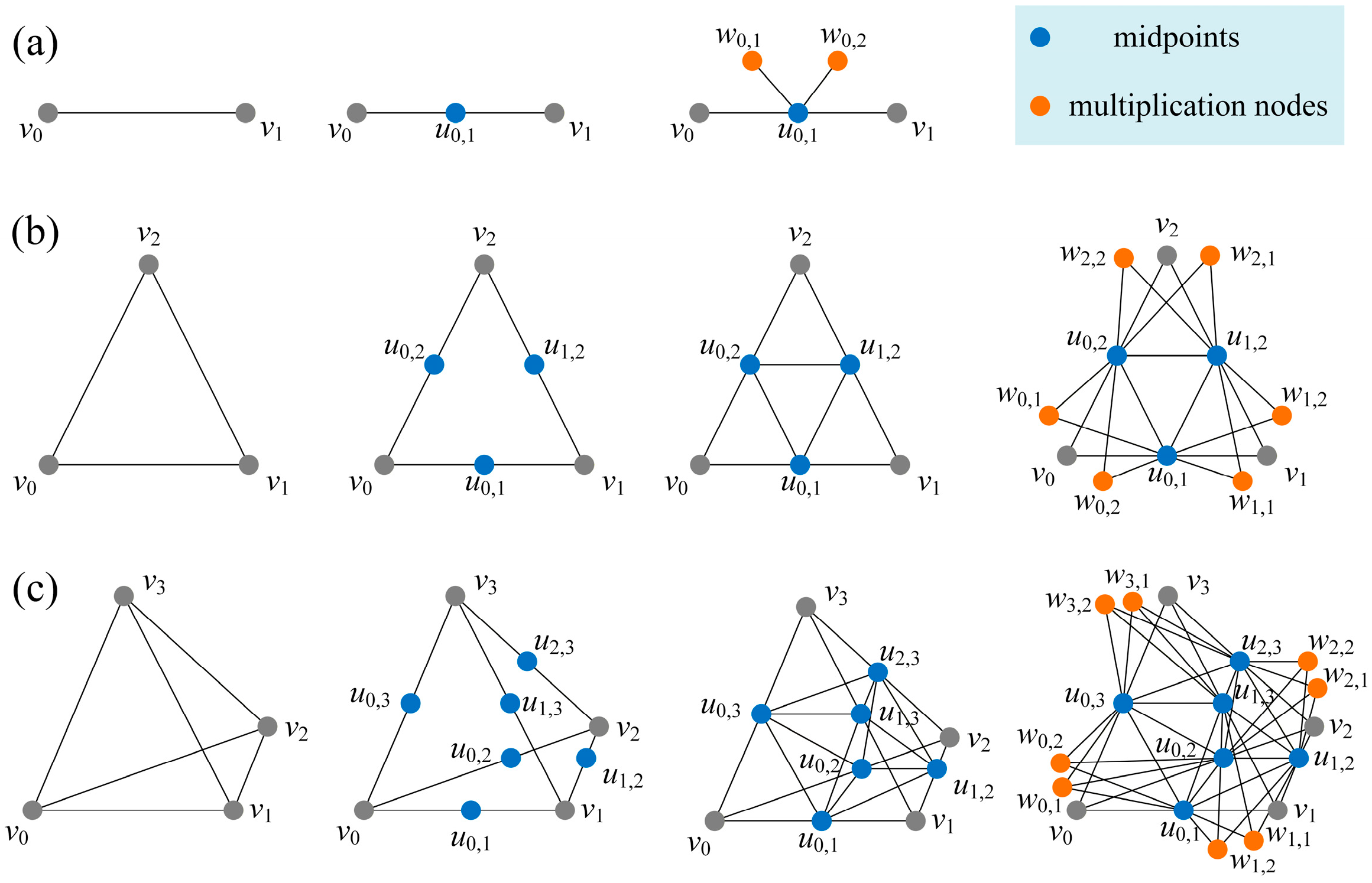
First, a network consisting of nodes and edges is generated through an iterative process. Subsequently, certain cliques within the resulting network are treated as simplices to form a simplicial complex. The specific procedure is detailed below, as illustrated in Figure 1.

1. Initialization: Begin with a $\left(K+1\right)$-clique.

2. Iteration: For each $\left(K+1\right)$-clique $\sigma =[v_0,v_1,\dots ,v_K]$ present in the graph obtained from the previous iteration, execute the following steps sequentially:

(i) For every edge $[v_i,v_j]$ (where $0\le i<j\le K$) within $\sigma$, introduce a new node $u_{i,j}$. Remove the original edge $[v_i,v_j]$ and add two new edges $[v_i,u_{i,j}]$ and $[v_j,u_{i,j}]$. For clarity, this paper refers to the newly introduced node $u_{i,j}$ as a midpoint, and the edge $[v_i,v_j]$ at the previous iteration as the original edge corresponding to that midpoint.

(ii) For each original vertex $v_i$ (where $0\le i\le K$) of $\sigma$, connect all $K$ midpoints incident to it pairwise. These $K$ nodes thereby form a $K$-clique, denoted as ${\tau }_i$. For clarity, this paper refers to this $K$-clique ${\tau }_i$ as a bottom.

(iii) For each bottom ${\tau }_i$, introduce $m$ new nodes $w_{i,1}$, $w_{i,2}$,…, $w_{i,m}$. Connect each node $w_{i,j}$ to all nodes within ${\tau }_i$. For clarity, this paper refers to the parameter $m$ as the multiplier, and the newly introduced nodes $w_{i,1}$, $w_{i,2}$,…, $w_{i,m}$ as multiplication nodes.

After $t$ iterations, the resulting graph is denoted as ${\mathcal{G}}_t(K,m)=\left\{{\mathcal{V}}_t,{\mathcal{E}}_t\right\}$, where ${\mathcal{V}}_t$ is the vertex set and ${\mathcal{E}}_t$ is the edge set.

3. Generating the Higher-Order Network (Simplicial Complex): Each $\left(K+1\right)$-clique in the graph ${\mathcal{G}}_t(K,m)$ is considered a $K$-simplex. The collection of all such $K$-simplices and their faces constitutes a simplicial complex, denoted as ${\mathcal{K}}_t(K,m)$.

The simplicial complex ${\mathcal{K}}_t\left(K,m\right)$ constitutes a pure $K$-dimensional simplicial complex, as it consists of a set of $K$-simplices and their faces. We obtain a simplicial complex ${\mathcal{K}}_t\left(K,m\right)$ governed by three parameters: the dimension $K$ of the simplicial complex, the multiplier $m$, and the iteration count $t$. The graph ${\mathcal{G}}_t\left(K,m\right)$ is its 1-skeleton.

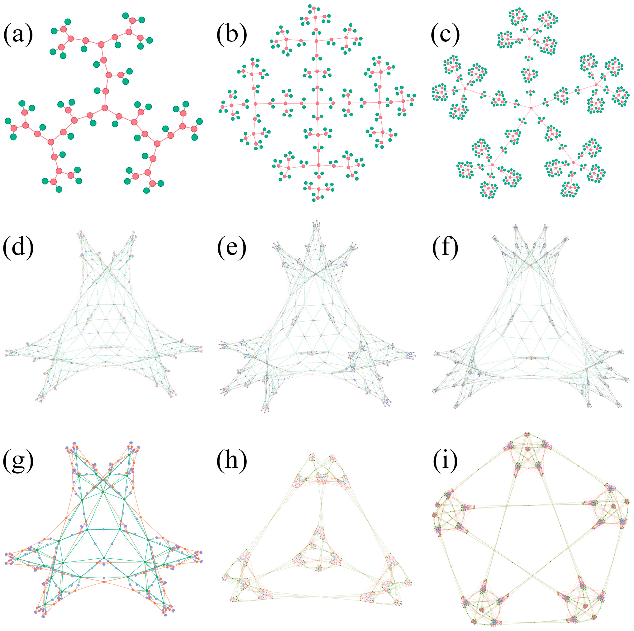
One advantage of this model is the flexible choice of the dimension $K$, allowing the generation of simplicial complexes of various dimensions, as illustrated in Figure 2.

For clarity,

Table 1. List of symbols.

Symbol	Description	Defined in
$k_{K,L}\left(\beta \right)$	The generalized degree of $L$-simplex $\beta$	Section 3.1.3
$P_{K,L}\left(k\right)$	$L$ dimensional generalized degree distribution of a pure $K$ dimensional simplicial complex	Section 3.1.3
${\mathcal{K}}_t\left(K,m\right)$	The pure simplicial complex obtained when the dimension is $K$, the multiplier is $m$, and the iteration count is $t$	Section 3.2
${\mathcal{G}}_t\left(K,m\right)$	The 1-skeleton of ${\mathcal{K}}_t\left(K,m\right)$	Section 3.2
$S$	The number of $K$-simplices contained in ${\mathcal{K}}_t\left(K,m\right)$ at iteration $t=1$	Section 4.1
$d_s$	Similarity dimension	Section 4.2.1
$d_B^{CBB}$	Box-counting dimension obtained using the compact-box-burning (CBB) algorithm	Section 4.2.2
$d_B^{OBCA}$	Box-counting dimension obtained using the overlapping box (OBCA) algorithm	Section 4.2.2
$Y_K\left(L,t,r\right)$	The number of $L$-simplices at iteration $t$ with generalized degree $k_{K,L}={(m+1)}^r$ for $K\ge 3$ and $L=1,2,\dots ,K-1$, and the number of $K$-simplices for $L=K$	Section 4.3
$N_K\left(t,k\right)$	The number of 0-simplices at iteration $t$ with generalized degree $k_{K,0}=k$ for $K\ge 3$	Section 4.3
$c_{L,r}$	The growth rate of the number of $L$-simplices with generalized degree $k_{K,L}={(m+1)}^r$	Section 4.3
$C_L$	The ratio of the number of $L$-simplices with generalized degree 1 and $m+1$	Section 4.3
$\gamma$	Power-law exponent of the $L$-dimensional generalized degree distribution, $L=1,2,\dots ,K-1$	Section 4.3
${\gamma }^{\prime }$	Power-law exponent of the 0-dimensional generalized degree distribution	Section 4.3

summarizes the mathematical symbols used throughout this paper and their corresponding meanings.

4. Properties

This section investigates certain properties of the higher-order network ${\mathcal{K}}_t\left(K,m\right)$ to elucidate its essential characteristics. Specifically, we focus on three properties: the number of $K$-simplices, the fractal dimension, and the generalized degree distribution. This is primarily because (1) the number of $K$-simplices represents the primary metric for characterizing the scale of the network ${\mathcal{K}}_t\left(K,m\right)$; (2) we shall demonstrate below that ${\mathcal{K}}_t\left(K,m\right)$ is fractal, and the fractal dimension describes the dynamic evolution of fractal networks, hence requiring its computation; (3) analyzing the generalized degree distributions of higher-order networks reveals whether they exhibit scale-free characteristics [36].

4.1. The Number of $K$-Simplices

According to the iterative generation rules of the network, the number of $K$-simplices grows exponentially. Let $S$ denote the number of $K$-simplices contained in ${\mathcal{K}}_t\left(K,m\right)$ at iteration $t=1$. In each iteration, the number of $K$-simplices in ${\mathcal{K}}_{t+1}\left(K,m\right)$ at iteration $t+1$ is $S$ times that in iteration $t$. This is because each $K$-simplex at iteration $t$ will transform into a simplicial complex composed of $S K$-simplices at the next iteration. Therefore, the number of $K$-simplices in ${\mathcal{K}}_t\left(K,m\right)$ is $S^t$. $S$ depends on the dimension $K$ and multiplier $m$, and its explicit form is given in Equation (1) of Proposition 1.

Proposition 1. 

The number of $K$-simplices contained in ${\mathcal{K}}_t\left(K,m\right)$ at iteration $t=1$ is $S$, and

$$S=\left\{\begin{array}{cc}m+2,& K=1,\\ 3m+4,& K=2,\\ \left(m+1\right)\left(K+1\right),& K>2.\end{array}\right.$$

(1)

Proof. 

This is because the $K$-simplices in the ${\mathcal{K}}_1\left(K,m\right)$ can be divided into three categories, namely (1) $K$-simplices formed by a vertex at iteration $t=0$ and the midpoints inserted at iteration $t=1$; (2) $K$-simplices formed between midpoints; and (3) the $K$-simplices formed by the bottom and the multiplication nodes.

(1) In the network ${\mathcal{K}}_1(K,m)$, for any node $v_i$ existing at $t=0$, the network construction step 2 (ii) defines $K$ midpoints connected to that node, and these midpoints are pairwise connected. Therefore, the node $v_i$ together with these $K$ midpoints forms a $K$-simplex. Because there are $K+1$ nodes at $t=0$, the number of such $K$-simplices is $K+1$.

(2) When $K=1$, the single midpoint $u_{0,1}$ in ${\mathcal{K}}_1(1,m)$ cannot form a 1-simplex. The number is 0.

When $K=2$, as shown in Figure 1b, the three midpoints in ${\mathcal{K}}_1(2,m)$ are pairwise connected, forming one 2-simplex. The number is 1.

When $K\ge 3$, we prove that no $K$-simplex can be formed solely by the midpoints. Assume there exists a $K$-simplex $U$ composed of $K+1$ midpoints. These $K+1$ midpoints are pairwise connected, which implies that the $K+1$ edges from $t=0$ corresponding to them pairwise share a common vertex. Let $E(U)$ be the set of edges from $t=0$ corresponding to the midpoints in $U$, then $\left|E(U)\right|=K+1\ge 4$. Clearly, $E(U)$ is a set of distinct edges (because the midpoints in $U$ are distinct), and any two edges in it share a common vertex (because the corresponding midpoints are connected). Therefore, by Lemma A1 in Appendix A (which states that for a set containing at least four distinct edges, if every pair of edges shares a common vertex, then all edges share a common vertex), all edges in $E(U)$ must share a common vertex $v^{\ast }$. However, at $t=0$, the degree of any vertex is $K$, meaning that there are exactly $K$ edges incident to vertex $v^{\ast }$. This contradicts the fact that $E(U)$ contains $K+1$ edges. Hence, when $K\ge 3$, there is no $K$-simplex formed solely by the midpoints.

(3) When $K=1$, as shown in Figure 1a, ${\mathcal{K}}_1(K,m)$ has only one bottom. Each bottom is connected to $m$ multiplication nodes, forming $m$ 1-simplices.

When $K\ge 2$, as shown in Figure 1b,c, ${\mathcal{K}}_1(K,m)$ has $K+1$ bottoms. Each bottom connects to $m$ multiplication nodes, resulting in $m(K+1)$$K$-simplices.

Summing the counts from the three categories yields Formula (1). □

4.2. Fractal Dimension

Fractal dimension is a crucial parameter for describing the dynamic evolution of fractal networks. Numerous methods exist for calculating fractal dimensions within fractal geometry. One classic approach is the similarity dimension, which is frequently employed for regular self-similar geometric figures. In network science, there exist definitions for fractal networks and the box-counting dimension.

4.2.1. Similarity Dimension

If a whole set $\mathcal{A}$ can be partitioned into $N$ subsets of equal size, each of which is similar to $\mathcal{A}$ by a similarity ratio $a$, then the similarity dimension $d_s$ of $\mathcal{A}$ is defined as $d_s=\underset{a\to 0}{\lim }\left(\log N/\log \left(1/a\right)\right)=-\underset{a\to 0}{\lim }\left(\log N/\log a\right)$. According to the iterative generation rule of the network, in each iteration, every $K$-simplex is replaced by a subgraph that is structurally identical to ${\mathcal{K}}_1(K,m)$. Consequently, the network ${\mathcal{K}}_t(K,m)$ naturally consists of $S$ subgraphs that are structurally identical to ${\mathcal{K}}_{t-1}(K,m)$, and the diameter of each subgraph is half that of the whole. Furthermore, for any $n=1,2,3,\dots ,t$, the graph ${\mathcal{K}}_t(K,m)$ can be partitioned into $S^n$ subgraphs that are structurally identical to ${\mathcal{K}}_{t-n}(K,m)$, and the diameter of each subgraph is $1/2^n$ of the diameter of ${\mathcal{K}}_t(K,m)$. Therefore, the similarity dimension $d_s$ of ${\mathcal{K}}_t\left(K,m\right)$ is

$$d_s =-\underset{n\to \infty }{\lim }{\displaystyle \frac{\log S^n}{\log 1/2^n}}={\displaystyle \frac{\log S}{\log 2}},$$

(2)

where $S$ is given by Equation (1). For $K=1$, $d_s=\log \left(m+2\right)/\log 2$; for $K=2$, $d_s=\log \left(3m+4\right)/\log 2$; and for $K\ge 3$, $d_s=\log ((m+1)(K+1))/\log 2$. The theoretical value of the fractal dimension of the network, namely its similarity dimension, varies with two given parameters: the dimension $K$ of the simplicial complex and the multiplier $m$. Consequently, the fractal dimension of the higher-order fractal networks proposed in this study is controllable.

4.2.2. Box-Counting Dimension

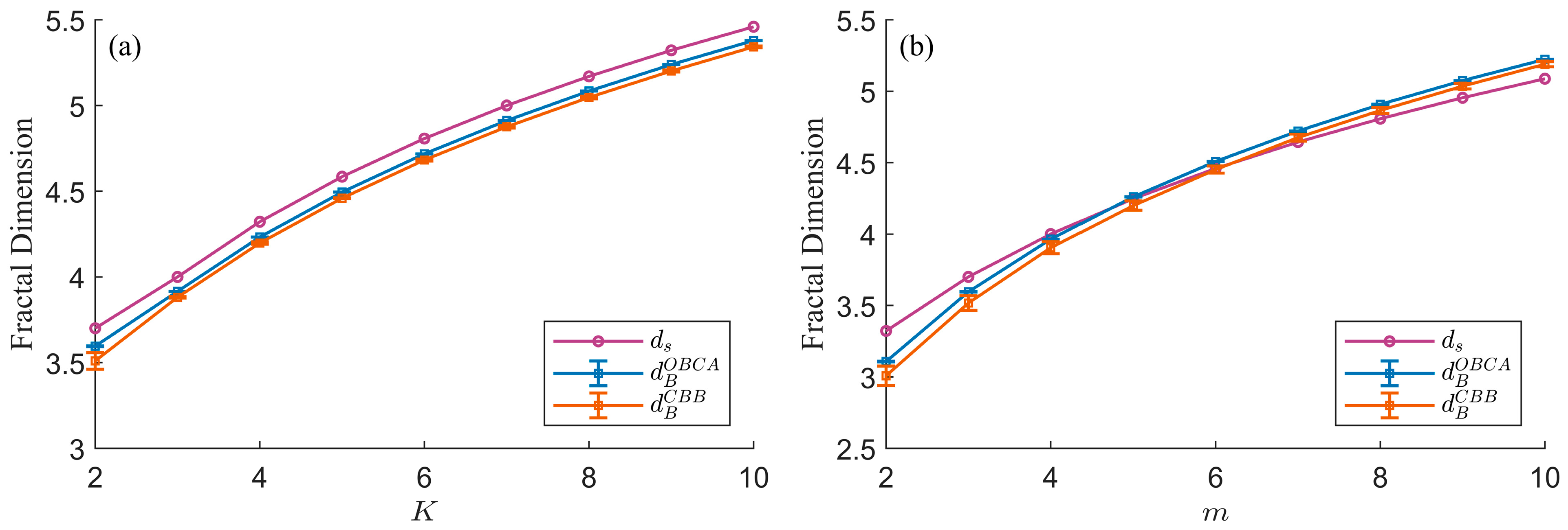
In the box-counting dimension, a box is a set of nodes in which the distance $l_{ij}$ between any two nodes $i$ and $j$ is less than the box size ${\mathcal{l}}_B$. For a given box size ${\mathcal{l}}_B$, the minimum number of boxes required to cover the network $\mathcal{G}$ is denoted by $N_B$. If a finite number $d_B$ exists such that $N_B\sim {\mathcal{l}}_B^{-d_B}$, then the network $\mathcal{G}$ is termed a fractal network, and $d_B$ is the box-counting dimension [1,9]. The determination of the minimum number of boxes $N_B$ for a given size ${\mathcal{l}}_B$ is an NP-hard problem [37]. Various box-covering algorithms have been proposed to calculate the number of boxes needed to cover a network [38,39,40]. Based on whether the central node of the box is preselected, typical algorithms for computing box-counting dimensions are categorized into two types [41]. The CBB algorithm [38] and the OBCA [39] are representative methods that select central nodes and do not select central nodes, respectively. Using the CBB and OBCA algorithms under various combinations of the two parameters $K$ and $m$, the fractal characteristics of the network were verified by averaging 100 independent replicate experiments [42]. The resulting $d_B^{CBB}$ and $d_B^{OBCA}$ values are shown in Figure 3. The computed box-counting dimensions are close to the similarity dimension, with the discrepancy arising from the box-covering algorithm.

4.3. Generalized Degree Distribution

The generalized degrees are the fundamental combinatorial properties that characterize the structure of simplicial complexes [19], and their distribution serves as the statistical basis for understanding the coupling between higher-order network structure and function. Specifically, the generalized degree distribution modulates the macroscopic dynamical behavior of the system. For example, Long et al. [43] pointed out that the epidemic transmission thresholds are related to the generalized degree distribution in the context of their proposed simplicial complex model. This finding suggests that characterizing the generalized degree distribution is a necessary prerequisite for linking the higher-order network topology to its macroscopic dynamics. Below, we analyze the generalized degree distribution of $L$-simplices ($L=0,1,2,\dots ,K-1$) in the network $K_t(K,m)$. We not only verify that the generalized degree distributions of simplices at various dimensions are scale-free, but also provide approximations of their power-law exponents to show how the parameters $K$ and $m$ control these distributions.

When $K=1$, the network ${\mathcal{K}}_t\left(1,m\right)$ is the graph ${\mathcal{G}}_t\left(1,m\right)$, which is a tree. Its generalized degree distribution $P_{1,0}\left(k\right)$ is a two-point distribution, as detailed in Appendix B.

When $K=2$, the 0-dimensional and 1-dimensional simplices in the network ${\mathcal{K}}_t\left(2,m\right)$ exhibit two and three possible values for their generalized degrees, respectively. The corresponding generalized degree distributions are given in Appendix B.

The following discussion focuses on the generalized degree distribution for $K\ge 3$. Propositions 2 and 3 characterize the generalized degrees and the iterative growth laws of 1- to $\left(K-1\right)$-dimensional and 0-dimensional simplices in the network ${\mathcal{K}}_t(K,m)$, respectively. Proposition 4 reveals the ratio relationships among different types of simplices (with different generalized degrees and dimensions). Propositions 5 and 6 determine approximate values of the power-law exponents for the generalized degree distributions of 1- to $\left(K-1\right)$-dimensional and 0-dimensional simplices in the network ${\mathcal{K}}_t(K,m)$, respectively. When $m$ is sufficiently large, the network ${\mathcal{K}}_t(K,m)$ constructed in this paper is scale-free.

Proposition 2. 

When $t\ge K$ and $1\le L\le K-1$, the generalized degree $k_{K,L}$ of an $L$-simplex in the network can take values of the form ${(m+1)}^r$ with $r=0,1,2,\dots ,K-L$. The generalized degree ${(m+1)}^r$ first occurs among $L$-simplices at iteration $r$. Let $Y_K\left(L,t,r\right)$ denote the number of $L$-simplices with generalized degree $k_{K,L}={(m+1)}^r$ at iteration $t$, and let $Y_K\left(K,t,0\right)$ denote the number of $K$-simplices. Then:

For $t=0$ and $L=1,2,\dots ,K$,

$$Y_K(L,0,r)=\left\{\begin{array}{ll}\left(\begin{array}{c}K+1\\ L+1\end{array}\right),\hfill & r=0,\hfill \\ 0,\hfill & \mathrm{otherwise}.\hfill \end{array}\right.$$

(3)

For $t\ge 0$ and $L=K$,

$$Y_K(K,t,r)=\left\{\begin{array}{ll}{S}^t,\hfill & r=0,\hfill \\ 0,\hfill & \mathrm{otherwise}.\hfill \end{array}\right.$$

(4)

For $t\ge 1$ and $L=1,2,\dots ,K-1$,

$$Y_K(L,t,r)=\left\{\begin{array}{ll}(L+1)Y_K(L,t-1,r)+(L+2)Y_K(L+1,t-1,r-1),\hfill & r=1,2,\dots ,K-L,\hfill \\ (L+1)Y_K(L,t-1,r)+m\cdot (K+1)\cdot S^{t-1}\cdot \left(\begin{array}{c}K\\ L\end{array}\right),\hfill & r=0,\hfill \\ 0,\hfill & \mathrm{otherwise},\hfill \end{array}\right.$$

(5)

 or, equivalently,

$$Y_K(L,t,r)=\left\{\begin{array}{ll}(L+1)Y_K(L,t-1,r)+(L+2)Y_K(L+1,t-1,r-1),\hfill & r=1,2,\dots ,K-L,\hfill \\ \left(\begin{array}{c}K+1\\ L+1\end{array}\right)S^t-{\displaystyle \sum _{j=1}^{K-L}{(m+1)}^j}\cdot Y_K(L,t,j),\hfill & r=0,\hfill \\ 0,\hfill & \mathrm{otherwise}.\hfill \end{array}\right.$$

(6)

Equation (5) describes the iterative law governing the number of simplices in the network, which are classified according to their generalized degree $k_{K,L}={(m+1)}^r$ with $r=0,1,2,\dots ,K-L$. The three terms in Equation (5) for $Y_K(L,t,r)$ are $(L+1)Y_K(L,t-1,r)$, $(L+2)Y_K(L+1,t-1,r-1)$, and $m(K+1)S^{t-1}\left(\begin{array}{c}K\\ L\end{array}\right)$. These correspond respectively to the three ways of obtaining an $L$-simplex through network iteration. Taking $K=3$, $m=1$, and $L=2$ as an example, the 2-simplices at iteration $t$ can be classified into the following three types:

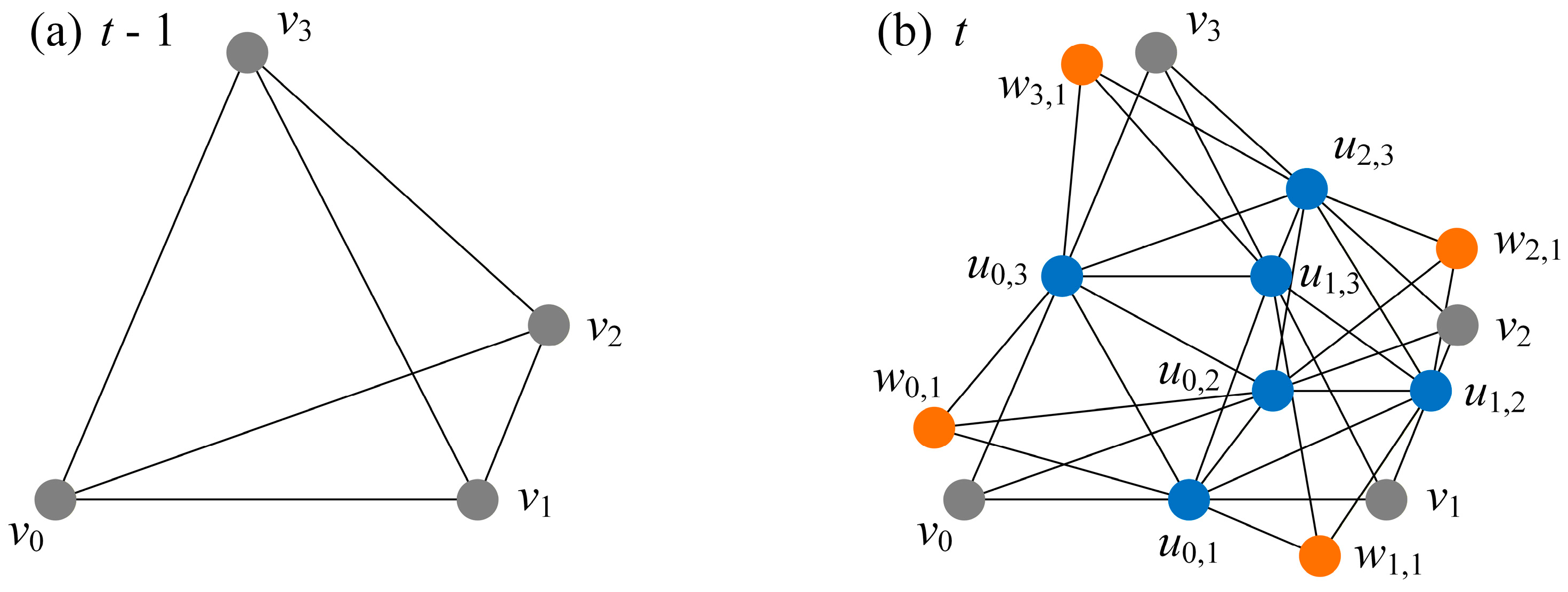
(1) Corresponding to the term $(L+1)Y_K(L,t-1,r)$: For instance, the 2-simplex $[v_0,v_1,v_2]$ in Figure 4a is subdivided into three 2-simplices, $[v_0,u_{0,1},u_{0,2}]$, $[v_1,u_{0,1},u_{1,2}]$, and $[v_2,u_{0,2},u_{1,2}]$, at the next iteration (Figure 4b). Their generalized degrees are all equal to that of $[v_0,v_1,v_2]$, which is 1. Note that the three nodes $u_{0,1}$, $u_{0,2}$, and $u_{1,2}$ do not form a 2-simplex because they are not a subset of any 3-simplex.

(2) Corresponding to the term $(L+2)Y_K(L+1,t-1,r-1)$: For example, the 3-simplex $[v_0,v_1,v_2,v_3]$ in Figure 4a gives rise to four 2-simplices formed by the midpoints at the next iteration (Figure 4b): $[u_{0,1},u_{0,2},u_{0,3}]$, $[u_{0,1},u_{1,2},u_{1,3}]$, $[u_{0,2},u_{1,2},u_{2,3}]$, and $[u_{0,3},u_{1,3},u_{2,3}]$. Their generalized degree is 2, which is twice the number of 3-simplices associated with $[v_0,v_1,v_2,v_3]$.

(3) Corresponding to the term $m(K+1)S^{t-1}\left(\begin{array}{c}K\\ L\end{array}\right)$: For example, in Figure 4b, there are twelve 2-simplices formed by the midpoints and the multiplication nodes, each with a generalized degree of 1 (e.g., $[w_{0,1},u_{0,1},u_{0,2}]$ is contained only in the 3-simplex $[w_{0,1},u_{0,1},u_{0,2},u_{0,3}]$).

Table 2. Evolution of simplex counts for the network ${\mathcal{K}}_t(3,1)$.

$\mathit{t}$	${\mathit{Y}}_{\mathbf{3}}\mathbf{(}\mathbf{3}\mathbf{,}\mathit{t}\mathbf{,}\mathit{r}\mathbf{)}$	${\mathit{Y}}_{\mathbf{3}}\mathbf{(}\mathbf{2}\mathbf{,}\mathit{t}\mathbf{,}\mathit{r}\mathbf{)}$		${\mathit{Y}}_{\mathbf{3}}\mathbf{(}\mathbf{1}\mathbf{,}\mathit{t}\mathbf{,}\mathit{r}\mathbf{)}$			${\mathit{N}}_{\mathbf{3}}\mathbf{(}\mathit{t}\mathbf{,}\mathit{k}\mathbf{)}$
	$\mathit{r}\mathbf{=}\mathbf{0}$	$\mathit{r}\mathbf{=}\mathbf{0}$	$\mathit{r}\mathbf{=}\mathbf{1}$	$\mathit{r}\mathbf{=}\mathbf{0}$	$\mathit{r}\mathbf{=}\mathbf{1}$	$\mathit{r}\mathbf{=}\mathbf{2}$	${\mathit{k}}_{\mathbf{3}\mathbf{,}\mathbf{0}}\mathbf{=}\mathbf{1}$	${\mathit{k}}_{\mathbf{3}\mathbf{,}\mathbf{0}}\mathbf{=}\mathbf{4}$	${\mathit{k}}_{\mathbf{3}\mathbf{,}\mathbf{0}}\mathbf{=}\mathbf{8}$	${\mathit{k}}_{\mathbf{3}\mathbf{,}\mathbf{0}}\mathbf{=}\mathbf{16}$
0	1	4	0	6	0	0	4	0	0	0
1	8	24	4	24	12	0	8	6	0	0
2	64	168	44	144	96	12	40	30	12	0
3	512	1272	388	1056	696	156	296	174	108	12

provides an example of the evolution of the number of simplices over time in the network ${\mathcal{K}}_t(K,m)$.

Proof. 

When $t=0$, each $L$-simplex (where $L=1,2,\dots ,K-1$) in the network ${\mathcal{K}}_t\left(K,m\right)$ is contained within exactly one $K$-simplex. and their number is $\left(\begin{array}{c}K+1\\ L+1\end{array}\right)$. Consequently, at $t=0$, the number of $L$-simplices with generalized degree $k_{K,L}=1$ is $\left(\begin{array}{c}K+1\\ L+1\end{array}\right)$, and the number of $L$-simplices with other values of $k_{K,L}$ is zero.

When $t\ge 1$, an $L$-simplex $\alpha$ (with $L=1,2,\dots ,K-1$) in the network is categorized into the following three types, based on the composition of its $L+1$ vertices:

(1) $\alpha$ consists of a node at iteration $t-1$ and $L$ nodes at the bottom at iteration $t$.

In this case, $\alpha$ is generated from an $L$-simplex ${\alpha }^{\prime }$ at iteration $t-1$, through the partitioning of ${\alpha }^{\prime }$ by inserting midpoints along its edges. The simplex $\alpha$ consists of one vertex of ${\alpha }^{\prime }$ and the $L$ adjacent midpoints. Consequently, the number of $K$-simplices containing $\alpha$ equals that containing ${\alpha }^{\prime }$, i.e., $k_{K,L}\left(\alpha \right)=k_{K,L}\left({\alpha }^{\prime }\right)$. The number of such $L$-simplices at iteration $t$ is $L+1$ times the number of $L$-simplices with the same generalized degree at iteration $t-1$.

(2) $\alpha$ consists of $L+1$ nodes in a bottom at iteration $t$.

In this case, the vertices of $\alpha$ are the $L+1$ midpoints adjacent to a single vertex of $\beta$, where $\beta$ is an $(L+1)$-simplex at iteration $t-1$. As $\alpha$ is contained within a bottom at iteration $t$, $\alpha$ is connected to $m$ multiplication nodes and one node from iteration $t-1$. Thus, its generalized degree is $k_{K,L}\left(\alpha \right)=(m+1)\cdot k_{K,L+1}\left(\beta \right)$. The number of $L$-simplices obtained in this manner is $L+2$ times the number of $(L+1)$-simplices from the previous moment.

(3) $\alpha$ consists of $L$ nodes in a bottom at iteration $t$ and one multiplied node connected to this bottom.

For $\alpha$, we have $k_{K,L}\left(\alpha \right)=1$ because $\alpha$ is contained only in the $K$-simplex formed by this multiplication node and the bottom. The number of $L$-simplices of this type is $m\cdot (K+1)\cdot \left(\begin{array}{c}K\\ L\end{array}\right)$ times the number of $K$-simplices at the previous iteration. Moreover, the number of $L$-simplices of this type can be calculated as the total number of $L$-simplices minus the sum, over all other generalized degrees, of the product of the number of $L$-simplices and their corresponding generalized degree.

For a $(K-1)$-simplex $\alpha$ at iteration $t-1$, if $\alpha$ is a bottom, then its generalized degree $k_{K,K-1}\left(\alpha \right)=m+1$; otherwise, $k_{K,K-1}\left(\alpha \right)=1$.

Synthesizing the above analysis completes the proof of Proposition 2. □

Proposition 3. 

Let the number of 0-simplices with generalized degree $k_{K,0}=k$ at iteration $t$ be denoted by $N_K\left(t,k\right)$, then for $t\ge 1$

$$N_K(t,k)=\left\{\begin{array}{ll}{N}_K(t-1,k)+m(K+1)S^{t-1},\hfill & k=1,\hfill \\ N_K(t-1,k)+Y_K(1,t-1,r-1),\hfill & k\in \{2{(m+1)}^r\mid r=1,2,\dots ,K\},\hfill \\ 0,\hfill & \mathrm{otherwise},\hfill \end{array}\right.$$

(7)

and

$$N_K(0,k)=\left\{\begin{array}{ll}K+1,\hfill & k=1,\hfill \\ 0,\hfill & \mathrm{otherwise}.\hfill \end{array}\right.$$

(8)

Equation (7) describes the iterative evolution of the number of nodes (0-simplices) in the network ${\mathcal{K}}_t(K,m)$, which are classified by their generalized degree. The expression $N_K(t,k)$ contains three terms: $N_K(t-1,k)$, $m(K+1)S^{t-1}$, and $Y_K\left(1, t-1, r-1\right)$. These correspond to the three possible origins of a node with generalized degree $k$ at iteration $t$: (1) Pre-existing nodes. These are nodes that are already present at iteration $t-1$. For example, as illustrated in Figure 4, the four nodes, $v_0$, $v_1$, $v_2$, and $v_3$, have a generalized degree of 1 at iteration $t-1$, and they retain this degree of 1 at the subsequent iteration $t$. (2) New midpoints. For example, the midpoint $u_{0,1}$ created at iteration $t$ in Figure 4b is contained in four 3-simplices: $[v_0,u_{0,1},u_{0,2},u_{0,3}]$, $[w_{0,1},u_{0,1},u_{0,2},u_{0,3}]$, $[v_1,u_{0,1},u_{1,2},u_{1,3}]$, and $[w_{1,1},u_{0,1},u_{1,2},u_{1,3}]$. Its generalized degree is $2\left(m+1\right)=4$ times that of the edge $[v_0,v_1]$ at iteration $t-1$. (3) New multiplication nodes. In Figure 4b, the multiplication nodes $w_{0,1}$, $w_{1,1}$, $w_{2,1}$, and $w_{3,1}$ all have a generalized degree of 1 (e.g., $w_{0,1}$ is contained only in the 3-simplex $[w_{0,1},u_{0,1},u_{0,2},u_{0,3}]$). The data presented in Table 2 provides a numerical verification for the above mechanisms.

Proof. 

For a 0-simplex $\alpha$ at iteration $t$, the following three possibilities exist:

(1) $\alpha$ existed at the previous iteration, and its generalized degree $k_{K,0}(\alpha )$ remains unchanged; (2) if $\alpha$ is a newly inserted midpoint at iteration $t$ on an edge $\beta$, its generalized degree $k_{K,0}(\alpha )$ is $2(m+1)$ times that of $\beta$ at iteration $t-1$; (3) $\alpha$ is the multiplication node at this iteration, it is contained in one $K$-simplex formed by $\alpha$ and a bottom, yielding $k_{K,0}(\alpha )=1$. In summary, this completes the proof of Equation (7). □

In the recurrence relation given by Equation (5), when $r=0$, the expression for $Y_K(L,t,r)$ contains a term proportional to $S^{t-1}$. Since $S=(m+1)(K+1)>L+1>1$, the exponential growth pattern associated with this term dominates the long-term behavior of $Y_K(L,t,0)$, so its asymptotic form can be written as $Y_K(L,t,0)\approx c_{L,0}{S}^t$. Furthermore, this exponential growth pattern recursively determines the long-term behavior of $Y_K(L,t,r)$ for all higher values of $r$ (where $1\le r\le K-L$) through the recurrence relations in Equation (5). Therefore, for any $r=0,1,2,\dots ,K-L$, we have $Y_K(L,t,r)\approx c_{L,r}{S}^t$.

Proposition 4. 

The ratio of the number of $L$-simplices with different generalized degrees tends to a constant. Let $C_L$ denote the ratio of the number of $L$-simplices with generalized degree $1$ to that with generalized degree $m+1$. Then

$$C_L={\displaystyle \frac{(S-L-2)(L+1)}{(K-L)(L+2)}},$$

(9)

and the ratio of the number of $L$-simplices with generalized degree ${(m+1)}^r$ to those with generalized degree ${(m+1)}^{r+1}$ is given by $C_{L+r}$, namely

$${\displaystyle \frac{Y_K(L,t,r)}{Y_K(L,t,r+1)}}=C_{L+r}.$$

(10)

Proof. 

Substituting $Y_K(L,t,r)\approx c_{L,r}{S}^t$ into the branch of Equation (5) for $1\le r\le K-L$ yields

$$c_{L,r}{S}^t=(L+1)c_{L,r}{S}^{t-1}+(L+2)c_{L+1,r-1}{S}^{t-1}.$$

(11)

Rearranging the above expression yields that

$$c_{L,r}={\displaystyle \frac{L+2}{S-L-1}}{c}_{L+1,r-1},$$

(12)

where $L=1,2,\dots ,K-1$. In particular, $c_{L,1}={\displaystyle \frac{L+2}{S-L-1}}{c}_{L+1,0}$ for $r=1$.

Substituting $Y_K(L,t,r)\approx c_{L,r}{S}^t$ into the branch of Equation (6) for $r=0$ yields:

$$c_{L,0}{S}^t=\left(\begin{array}{c}K+1\\ L+1\end{array}\right)S^t-{\displaystyle \sum _{j=1}^{K-L}{(m+1)}^j}{c}_{L,j}{S}^t.$$

(13)

Dividing both sides of Equation (13) by $S^t$ yields

$$c_{L,0}=\left(\begin{array}{c}K+1\\ L+1\end{array}\right)-{\displaystyle \sum _{j=1}^{K-L}{(m+1)}^j}{c}_{L,j}.$$

(14)

Equation (14) is equivalent to

$${\displaystyle \sum _{j=0}^{K-L}{(m+1)}^j}{c}_{L,j}=\left(\begin{array}{c}K+1\\ L+1\end{array}\right).$$

(15)

Substituting Equation (12) into the right-hand side of Equation (14) and performing some straightforward arithmetic operations yields

$$\begin{array}{cc}\hfill c_{L,0} =& \left(\begin{array}{c}K+1\\ L+1\end{array}\right)-{\displaystyle \frac{L+2}{S-L-1}}\cdot (m+1){\displaystyle \sum _{j=0}^{K-L-1}{(m+1)}^j}{c}_{L+1,j}\hfill \\ \hfill =& \left(\begin{array}{c}K+1\\ L+1\end{array}\right)\cdot {\displaystyle \frac{m(L+1)}{S-L-1}}.\hfill \end{array}$$

(16)

By assumption $Y_K(L,t,r)\approx c_{L,r}{S}^t$, we have

$${\displaystyle \frac{Y_K(L,t,r)}{Y_K(L,t,r+1)}}={\displaystyle \frac{c_{L,r}}{c_{L,r+1}}},$$

(17)

and

$${\displaystyle \frac{Y_K(L+1,t,r-1)}{Y_K(L+1,t,r)}}={\displaystyle \frac{c_{L+1,r-1}}{c_{L+1,r}}}.$$

(18)

Substituting Equation (12) into the above ratios yields

$${\displaystyle \frac{Y_K(L,t,r)}{Y_K(L,t,r+1)}}={\displaystyle \frac{Y_K(L+1,t,r-1)}{Y_K(L+1,t,r)}}.$$

(19)

By the definition of $C_L$, we have $C_L=Y_K(L,t,0)/Y_K(L,t,1)$. Substituting $Y_K(L,t,r)\approx c_{L,r}{S}^t$ yields

$$C_L={\displaystyle \frac{c_{L,0}{S}^t}{c_{L,1}{S}^t}}.$$

(20)

Substituting Equation (12) into Equation (20) yields

$$C_L={\displaystyle \frac{S-L-1}{L+2}}\cdot {\displaystyle \frac{c_{L,0}}{c_{L+1,0}}}.$$

(21)

From Equation (16), the values of $c_{L,0}$ and $c_{L+1,0}$ can be determined. Substituting these values and rearranging yields Equation (9). The value of $C_L$ has been verified experimentally. Combining Equations (9) and (19) yields Equation (10), which has also been verified experimentally. □

Proposition 5. 

When $m$ is large, the generalized degree distribution $P_{K,L}\left(k\right)$ of $L$-simplices follows an approximate power law:

$$P_{K,L}(k)~k^{-\gamma }.$$

(22)

The corresponding power-law exponent $\gamma$ is approximately

$$\gamma \approx {\displaystyle \frac{1}{(K-L)\log (m+1)}}\log {\displaystyle \frac{L+1}{K+1}}\left(\begin{array}{c}S-L-2\\ K-L\end{array}\right).$$

(23)

Proof. 

For large $m$, we have $C_{L+r}={\displaystyle \frac{\left(S-L-r-2\right)\left(L+r+1\right)}{\left(K-L-r\right)\left(L+r+2\right)}}\approx {\displaystyle \frac{S}{K-L-r}}$. Thus,

$$Y_K(L,t,r)\approx Y_K(L,t,0)\cdot {\displaystyle \prod _{j=0}^{r-1}\frac{K-L-j}{S}},$$

(24)

and consequently

$$\log Y_K(L,t,r)\approx \log Y_K(L,t,0)+{\displaystyle \sum _{j=0}^{r-1}\log }{\displaystyle \frac{K-L-j}{S}}.$$

(25)

Because $\log {\displaystyle \frac{K-L-j}{S}}$ varies little with $j$, the following ratio also changes little with $r$:

$${\displaystyle \frac{\log P_{K,L}(k_{r+1})-\log P_{K,L}(k_r)}{\log k_{r+1}-\log k_r}}={\displaystyle \frac{\log \frac{Y_K(L,t,r+1)}{{\displaystyle \sum _j{Y}_K}(L,t,j)}-\log \frac{Y_K(L,t,r)}{{\displaystyle \sum _j{Y}_K}(L,t,j)}}{\log {(m+1)}^{r+1}-\log {(m+1)}^r}}=\log {\displaystyle \frac{Y_K(L,t,r+1)}{Y_K(L,t,r)}},$$

(26)

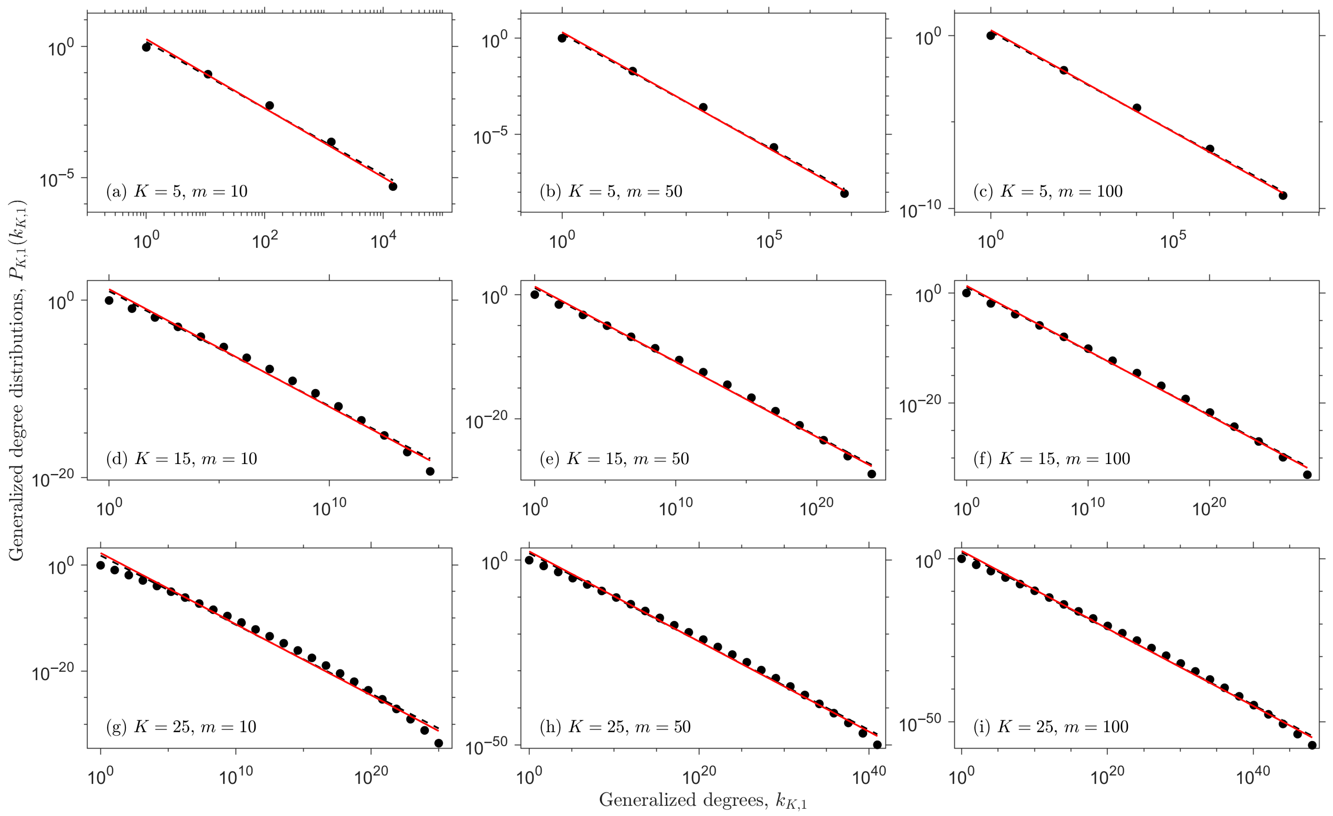
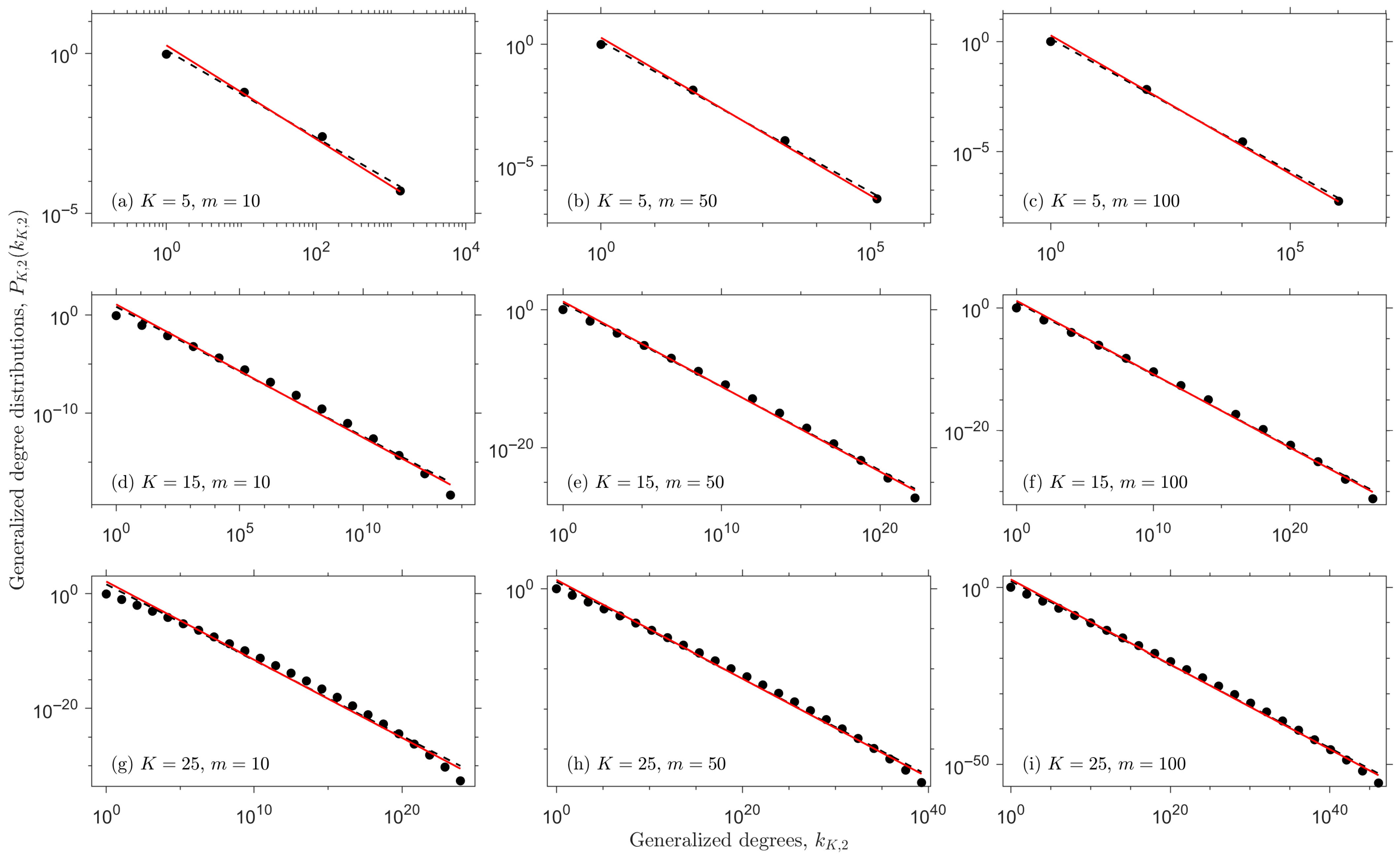
where $k_r={(m+1)}^r$ and $k_{r+1}={(m+1)}^{r+1}$. This implies that in the double-logarithmic coordinate system, $(k,P_{K,L}(k))$ approximates a linear distribution, as illustrated in Figure 5 and Figure 6. Consequently, the generalized degree distribution $P_{K,L}\left(k\right)$ exhibits an approximate scale-free behavior, i.e., Equation (22).

Based on the above analysis, we can estimate $\gamma$ by using the first and last points of the distribution as fitting targets. Combining Equations (9) and (10), the number of $L$-simplices with generalized degree $k=k_0={(m+1)}^0=1$ is given by

$$Y_K(L,t,0)\approx Y_K(L,t,K-L)\cdot {\displaystyle \prod _{j=L}^{K-1}{C}_j}={\displaystyle \frac{L+1}{K+1}}\cdot \left(\begin{array}{c}S-L-2\\ K-L\end{array}\right)\cdot Y_K(L,t,K-L),$$

(27)

thereby

$$\gamma \approx -{\displaystyle \frac{\log P_{K,L}({(m+1)}^{K-L})-\log P_{K,L}(1)}{\log {(m+1)}^{K-L}-\log 1}}.$$

(28)

Simplifying this expression yields $\gamma \approx {\displaystyle \frac{1}{\left(K-L\right)\log \left(m+1\right)}}\log {\displaystyle \frac{L+1}{K+1}}\left(\begin{array}{c}S-L-2\\ K-L\end{array}\right)$, which is Equation (23). Compared to the $\gamma$ value obtained by fitting all data points using the least squares method, the estimate derived from Equation (23) shows no significant difference, as illustrated in Figure 5 and Figure 6. The theoretical power-law exponent $\gamma$ is derived from the analysis of the long-term behavior of the network. For a finite number of iterations $t=30$, the theoretical line in the double-logarithmic plot may deviate from the raw data points because of finite-size effects. □

Proposition 6. 

When $m$ is large, the generalized degree distribution of 0-simplices $P_{K,0}\left(k\right)={\displaystyle \frac{N_K\left(t,k\right)}{{\displaystyle \sum _{k^{\prime }} }{N}_K\left(t,k^{\prime }\right)}}$ approximates a power-law distribution, namely

$$P_{K,0}(k)~k^{-{\gamma }^{\prime }},$$

(29)

where $k=1,2(m+1),2{(m+1)}^2,\dots ,2{(m+1)}^K$, and the approximate value of ${\gamma }^{\prime }$ is given by the value of Equation (23) when $L=1$, i.e.,

$${\gamma }^{\prime }\approx {\displaystyle \frac{1}{(K-1)\log (m+1)}}\log {\displaystyle \frac{2}{K+1}}\left(\begin{array}{c}S-3\\ K-1\end{array}\right).$$

(30)

Proof. 

Let $k_r=2{(m+1)}^r$. Then, from the recursive formula for $N_K\left(t,k\right)$ and the initial conditions, the number of 0-simplices with generalized degree $k_r$ at iteration $t$ is given by

$$N_K(t,k_r)={\displaystyle \sum _{t^{\prime }=0}^{t-1}{Y}_K}(1,t^{\prime },r-1).$$

(31)

From Equation (10), the ratio $Y_K\left(1,t,r-1\right)/Y_K\left(1,t,r\right)$ is approximately constant, denoted $C_r$. Furthermore, because $Y_K\left(1,t,r\right)$ grows exponentially with $t$, we have

$${\displaystyle \frac{N_K(t,k_r)}{N_K(t,k_{r+1})}}={\displaystyle \frac{{\displaystyle \sum _{t^{\prime }=0}^{t-1}{Y}_K}(1,t^{\prime },r-1)}{{\displaystyle \sum _{t^{\prime }=0}^{t-1}{Y}_K}(1,t^{\prime },r)}}\approx C_r.$$

(32)

Consequently, the generalized degree distribution of 0-simplices approximates a power law, with the power-law exponent ${\gamma }^{\prime }$ given above. The proof proceeds analogously to that for the generalized degree distribution of $L$-simplices. □

5. Conclusions

Modeling higher-order fractal networks is key to understanding the fractal characteristics emerging within complex systems with higher-order interactions. Here, we propose a general method for constructing higher-order fractal scale-free networks based on simplicial complexes. The constructed network ${\mathcal{K}}_t\left(K,m\right)$ is determined by the dimension $K$ of the simplicial complex, the multiplier $m$, and the iteration count $t$, which enables the dimension of the simplex complex to be specified arbitrarily. Theoretical analysis based on similarity dimensions and experimental verification using box-counting dimensions confirm that the generated networks exhibit fractal properties with controllable fractal dimensions. Furthermore, for large $m$, the generalized degree distribution of ${\mathcal{K}}_t\left(K,m\right)$ is scale-free, and the approximate value $\gamma$ of the power-law exponent has been determined.

Further work will explore higher-order fractal networks, particularly their topological features and dynamic behaviors.

References

1. Song, C.; Havlin, S.; Makse, H.A. Self-similarity of complex networks. Nature 2005, 433, 392–395. [Google Scholar] [CrossRef] [Scilit]
2. Yook, S.-H.; Radicchi, F.; Meyer-Ortmanns, H. Self-similar scale-free networks and disassortativity. Phys. Rev. E 2005, 72, 045105. [Google Scholar] [CrossRef] [Scilit] [PubMed]
3. Qi, L.; Guo, F.-Y.; Zhang, J.; Wang, Y.-W. An Internet review topic hierarchy mining method based on modified continuous renormalization procedure. Fractals 2022, 30, 2250134. [Google Scholar] [CrossRef] [Scilit]
4. Guo, F.; Qi, L.; Fan, Y. Attack vulnerability of fractal scale-free network. Fractals 2024, 32, 2450069. [Google Scholar] [CrossRef] [Scilit]
5. Deng, C.-F.; Yang, S.-H.; Xie, R.; Ju, X.-J.; Liu, Z.; Pan, D.-W.; Xu, J.; Luo, G.; Wang, W.; Chu, L.-Y. Flexible fractal integration of microfluidic modules for controllable mass production of monodisperse microdroplets. Ind. Eng. Chem. Res. 2023, 62, 12690–12702. [Google Scholar] [CrossRef] [Scilit]
6. Levine, J.M.; Bascompte, J.; Adler, P.B.; Allesina, S. Beyond pairwise mechanisms of species coexistence in complex communities. Nature 2017, 546, 56–64. [Google Scholar] [CrossRef] [Scilit]
7. Grilli, J.; Barabás, G.; Michalska-Smith, M.J.; Allesina, S. Higher-order interactions stabilize dynamics in competitive network models. Nature 2017, 548, 210–213. [Google Scholar] [CrossRef] [Scilit]
8. Sizemore, A.E.; Giusti, C.; Kahn, A.; Vettel, J.M.; Betzel, R.F.; Bassett, D.S. Cliques and cavities in the human connectome. J. Comput. Neurosci. 2018, 44, 115–145. [Google Scholar] [CrossRef] [Scilit]
9. Benson, A.R.; Gleich, D.F.; Leskovec, J. Higher-order organization of complex networks. Science 2016, 353, 163–166. [Google Scholar] [CrossRef] [Scilit]
10. Sizemore, A.E.; Karuza, E.A.; Giusti, C.; Bassett, D.S. Knowledge gaps in the early growth of semantic feature networks. Nat. Hum. Behav. 2018, 2, 682–692. [Google Scholar] [CrossRef] [Scilit]
11. Tadić, B.; Chutani, M.; Gupte, N. Multiscale fractality in partial phase synchronisation on simplicial complexes around brain hubs. Chaos Solitons Fractals 2022, 160, 112201. [Google Scholar] [CrossRef] [Scilit]
12. Luo, L.; Nian, F.; Cui, Y.; Li, F. Fractal information dissemination and clustering evolution on social hypernetwork. Chaos Interdiscip. J. Nonlinear Sci. 2024, 34, 093128. [Google Scholar] [CrossRef] [Scilit]
13. Jeong, H.; Mason, S.P.; Barabási, A.-L.; Oltvai, Z.N. Lethality and centrality in protein networks. Nature 2001, 411, 41–42. [Google Scholar] [CrossRef] [Scilit] [PubMed]
14. Lambiotte, R.; Rosvall, M.; Scholtes, I. From networks to optimal higher-order models of complex systems. Nat. Phys. 2019, 15, 313–320. [Google Scholar] [CrossRef] [Scilit] [PubMed]
15. Guo, F.; Qi, L.; Fan, Y. Cascading failure in fractal scale-free networks. Fractals 2025, 33, 2550039. [Google Scholar] [CrossRef] [Scilit]
16. Song, C.; Havlin, S.; Makse, H.A. Origins of fractality in the growth of complex networks. Nat. Phys. 2006, 2, 275–281. [Google Scholar] [CrossRef] [Scilit]
17. Rozenfeld, H.D.; Havlin, S.; ben-Avraham, D. Fractal and transfractal recursive scale-free nets. New J. Phys. 2007, 9, 175. [Google Scholar] [CrossRef] [Scilit]
18. Battiston, F.; Cencetti, G.; Iacopini, I.; Latora, V.; Lucas, M.; Patania, A.; Young, J.-G.; Petri, G. Networks beyond pairwise interactions: Structure and dynamics. Phys. Rep. 2020, 874, 1–92. [Google Scholar] [CrossRef] [Scilit]
19. Bianconi, G. Higher-Order Networks, 1st ed.; Cambridge University Press: Cambridge, UK, 2021. [Google Scholar]
20. Wang, J.-W.; Rong, L.-L.; Deng, Q.-H.; Zhang, J.-Y. Evolving hypernetwork model. Eur. Phys. J. B 2010, 77, 493–498. [Google Scholar] [CrossRef] [Scilit]
21. Liu, D.; Blenn, N.; Van Mieghem, P. A social network model exhibiting tunable overlapping community structure. Procedia Comput. Sci. 2012, 9, 1400–1409. [Google Scholar] [CrossRef] [Scilit]
22. Wu, Z.; Duan, J.; Fu, X. Synchronization of an evolving complex hyper-network. Appl. Math. Model. 2014, 38, 2961–2968. [Google Scholar] [CrossRef] [Scilit]
23. Bianconi, G.; Rahmede, C. Network geometry with flavor: From complexity to quantum geometry. Phys. Rev. E 2016, 93, 032315. [Google Scholar] [CrossRef] [Scilit]
24. Kawasaki, F.; Yakubo, K. Reciprocal relation between the fractal and the small-world properties of complex networks. Phys. Rev. E 2010, 82, 036113. [Google Scholar] [CrossRef] [Scilit]
25. Dorogovtsev, S.N.; Goltsev, A.V.; Mendes, J.F.F. Pseudofractal scale-free web. Phys. Rev. E 2002, 65, 066122. [Google Scholar] [CrossRef] [Scilit]
26. Ma, F.; Wang, P. Understanding influence of fractal generative manner on structural properties of tree networks. Chaos Solitons Fractals 2024, 180, 114523. [Google Scholar]
27. Vallee, N.; Monsuez, B. A formal model of SystemC components using fractal hypergraphs. In Proceedings of the International MultiConference of Engineers and Computer Scientists 2010, Hong Kong, China, 17–19 March 2010; Volume II, pp. 1418–1423. [Google Scholar]
28. Berec, V. Non-Abelian Topological Approach to Non-Locality of a Hypergraph State. Entropy 2015, 17, 3376–3399. [Google Scholar]
29. Ma, X.; Ma, F.; Yin, J. A fractal hypernetwork model with good controllability. AIMS Math. 2021, 6, 13758–13773. [Google Scholar] [CrossRef] [Scilit]
30. Zheng, S.; Man, X.; Kong, Z.-L.; Lin, Z.-K.; Duan, G.; Chen, N.; Yu, D.; Jiang, J.-H.; Xia, B. Observation of fractal higher-order topological states in acoustic metamaterials. Sci. Bull. 2022, 67, 2069–2075. [Google Scholar] [CrossRef] [Scilit] [PubMed]
31. Xie, Z.; Wang, Y.; Xu, W.; Zhu, L.; Li, W.; Zhang, Z. Combinatorial Properties for a Class of Simplicial Complexes Extended from Pseudo-fractal Scale-free Web. Fractals 2023, 31, 2350022. [Google Scholar]
32. Shang, Y. Sombor index and degree-related properties of simplicial networks. Appl. Math. Comput. 2022, 419, 126881. [Google Scholar] [CrossRef] [Scilit]
33. Stanley, R.P. Combinatorics and Commutative Algebra, 2nd ed.; Birkhäuser: Basel, Switzerland, 1996. [Google Scholar]
34. Rotman, J.J. An Introduction to Algebraic Topology, 1st ed.; Springer: Berlin/Heidelberg, Germany, 1998. [Google Scholar]
35. Bianconi, G.; Rahmede, C. Complex quantum network manifolds in dimension d > 2 are scale-free. Sci. Rep. 2015, 5, 13979. [Google Scholar] [CrossRef] [Scilit]
36. Barabasi, A.-L.; Albert, R. Emergence of scaling in random networks. Science 1999, 286, 509–512. [Google Scholar] [CrossRef] [Scilit]
37. Gallos, L.K.; Song, C.; Makse, H.A. A review of fractality and self-similarity in complex networks. Phys. A Stat. Mech. Its Appl. 2007, 386, 686–691. [Google Scholar] [CrossRef] [Scilit]
38. Song, C.; Gallos, L.K.; Havlin, S.; Makse, H.A. How to calculate the fractal dimension of a complex network: The box covering algorithm. J. Stat. Mech. Theory Exp. 2007, 2007, P03006. [Google Scholar] [CrossRef] [Scilit]
39. Sun, Y.; Zhao, Y. Overlapping-box-covering method for the fractal dimension of complex networks. Phys. Rev. E 2014, 89, 042809. [Google Scholar] [CrossRef] [Scilit] [PubMed]
40. Guo, F.-Y.; Zhou, J.-J.; Ruan, Z.-Y.; Zhang, J.; Qi, L. Hub-collision avoidance and leaf-node options algorithm for fractal dimension and renormalization of complex networks. Chaos Interdiscip. J. Nonlinear Sci. 2022, 32, 123116. [Google Scholar] [CrossRef] [Scilit]
41. Wen, T.; Cheong, K.H. The fractal dimension of complex networks: A review. Inf. Fusion 2021, 73, 87–102. [Google Scholar] [CrossRef] [Scilit]
42. Zakar-Polyák, E.; Nagy, M.; Molontay, R. Towards a better understanding of the characteristics of fractal networks. Appl. Netw. Sci. 2023, 8, 17. [Google Scholar] [CrossRef] [Scilit]
43. Long, T.; Tu, L.; Chen, J.; Wang, X.; Guo, Y. Contagion dynamics on growing simplicial complex networks via generalized degree vectors. Chaos Solitons Fractals 2025, 191, 115920. [Google Scholar] [CrossRef] [Scilit]
Figure 1. Schematic of the iterative process. In the figure, gray nodes v i are nodes existing at t = 0 , blue nodes u i , j are midpoints connected to vertices v i and v j at t = 1 , and orange nodes w i , k are multiplication nodes connected to the bottom. (a) K = 1 , m = 2 . The initial structure is a 2-clique. The iterative operations are (i) introduce the midpoint u 0 , 1 ; (ii) the midpoint u 0 , 1 constitutes the bottom; (iii) add m = 2 multiplication nodes w 0 , 1 and w 0 , 2 to the bottom. The simplicial complex K 1 ( 1 , 2 ) consists of four 1-simplices and their faces (i.e., all vertices). The four 1-simplices can be categorized into two types: edges connecting the bottom to nodes existing at t = 0 , and edges connecting the bottom to multiplication nodes. (b) K = 2 , m = 2 . The initial structure is a 3-clique. The iterative operations are:(i) introduce midpoints u 0 , 1 , u 0 , 2 , u 1 , 2 ; (ii) connect the midpoints adjacent to the same vertex pairwise, forming three bottoms [ u 0 , 1 , u 0 , 2 ] , [ u 0 , 1 , u 1 , 2 ] , and [ u 0 , 2 , u 1 , 2 ] ; (iii) for each bottom, add m = 2 multiplication nodes and connect them to all its vertices. The simplicial complex K 1 ( 2 , 2 ) consists of ten 2-simplices and their faces (i.e., all 1-simplices, or edges, and all 0-simplices, or vertices). Among the ten 2-simplices, three are formed by the bottoms and the nodes existing at t = 0 , six are formed by the bottoms and the multiplication nodes, and one is formed solely by the midpoints ( [ u 0 , 1 , u 0 , 2 , u 1 , 2 ] ). (c) K = 3 , m = 2 . The initial structure is a 4-clique. The iterative operations are (i) introduce midpoints u i , j ; (ii) for each node v i existing at t = 0 , connect pairwise the three midpoints connected to it, forming a bottom (e.g., the midpoints connected to v 0 form the bottom [ u 0 , 1 , u 0 , 2 , u 0 , 3 ] ); (iii) for each bottom, add m = 2 multiplication nodes and connect them to all its vertices. The simplicial complex K 1 ( 3 , 2 ) consists of twelve 3-simplices and their faces. The twelve 3-simplices are divided into two categories: four are formed by the bottoms, and the nodes at t = 0 (e.g., [ v 0 , u 0 , 1 , u 0 , 2 , u 0 , 3 ] ), and eight are formed by the bottoms and the multiplication nodes (e.g., [ w 0 , 1 , u 0 , 1 , u 0 , 2 , u 0 , 3 ] ).
Fractalfract 10 00306 g001
Figure 2. Networks obtained after multiple iterations. Nodes are colored differently to distinguish vertices with different generalized degrees. (ac) Networks after four iterations with K = 1 for m = 1 , 2 , 3 , respectively; (df) networks after four iterations with K = 2 for m = 1 , 2 , 3 , respectively; (gi) networks after three iterations with m = 1 for K = 2 , 3 , 4 , respectively.
Fractalfract 10 00306 g002
Figure 3. Fractal dimension of the network as a function of the simplicial complex dimension K and the multiplier m . (a) For a fixed multiplier m = 3 after t = 2 iterations, the fractal dimension is plotted against the simplicial complex dimension K ; (b) for a fixed simplicial complex dimension K = 2 and after t = 2 iterations, the fractal dimension is plotted against the multiplier m . The purple circles represent the theoretical similarity dimension d s . The blue and orange squares represent the box-counting dimensions d B O B C A and d B C B B , respectively, as computed by the OBCA and CBB algorithms. Each data point is the mean of 100 independent runs. Error bars correspond to ± 1 standard deviation.
Fractalfract 10 00306 g003
Figure 4. Evolution of a 3-simplex from iteration t 1 to t ( K = 3 , m = 1 ). In the figure, gray nodes v i are nodes existing at iteration t 1 , blue nodes u i , j are midpoints connected to vertices v i and v j at iteration t , and orange nodes w i , k are multiplication nodes connected to the bottom. (a) A 3-simplex in K t 1 ( 3 , 1 ) ; (b) the result of applying one iteration to the 3-simplex in (a), which is a subgraph of K t ( 3 , 1 ) .
Fractalfract 10 00306 g004
Figure 5. The 1-dimensional generalized degree distribution P K , 1 k for networks with t = 30 under different combinations of parameters K and m in a double-logarithmic coordinate system. The subplots are arranged by the parameter K (rows) and m (columns). The black circles represent the raw data points. The black dashed line is the ordinary least squares (OLS) fit to all data points ( log ( k ) , log ( P ) ) , whose negative slope is the fitted power-law exponent. The red solid line is the theoretical power-law line, whose slope is the negative of the theoretical power-law exponent γ calculated in this paper.
Fractalfract 10 00306 g005
Figure 6. The 2-dimensional generalized degree distribution P K , 2 k for networks with t = 30 under different combinations of parameters K and m in a double-logarithmic coordinate system. The subplots are arranged by the parameter K (rows) and m (columns). The black circles represent the raw data points. The black dashed line is the OLS fit to all data points ( log ( k ) , log ( P ) ) , whose negative slope is the fitted power-law exponent. The red solid line is the theoretical power-law line, whose slope is the negative of the theoretical power-law exponent γ calculated in this paper.
Fractalfract 10 00306 g006