On Uniformly δ-Geometric Convex Functions

Abstract

In this paper, we give some new Jensen, Jensen–Mercer, and Hermite–Hadamard inequalities for uniformly $\delta$-geometric convex functions. In addition, some limit bounds for Caputo–Fabrizio fractional integral operators are established as an application in the case of uniformly $\delta$-geometric convex functions. Some new examples and graphical representations are provided in order to illustrate the validity of our results.

1. Introduction

One of the old concepts of analysis that exists in the geometric shapes used by the ancient Greeks is convexity. But today, it is used in many fields of mathematics, such as probability theory, geometry, graph theory, coding and calculus of variations. In fact, due to the simple and understandable geometric understanding of this concept, it will be easy to analyze. For example, it is easily possible to interpret or recognize a convex function with the help of its graph and its epigraph. Therefore, many researchers today use the concept of convexity to define new functions that simplify their analysis. Convex functions are widely used in optimization theory and can also be used in finance. Convex functions are employed in portfolio optimization to reduce risk while optimizing expected return.

Convex theory and inequalities are closely related and are research fields of interest to many mathematicians, with many articles having been written in these fields. In recent years, some other kinds [1,2,3,4,5] of Hermite–Hadamard- [1,2,3,4], Jensen-, and Jensen–Mercer-type [5,6,7] inequalities have been established [8,9,10,11].

Jensen’s inequality was discovered in the 19th century by Johan Jensen, and later, in 2003, A. M. Mercer provided a significant refinement in [6]. A global bound for Jensen’s inequality was given in 2008 in [12]. In 2009, M. Niezgoda generalized Mercer’s inequality in [13], and in 2006, Pecaric et al. introduced the idea of the Mercer–Jensen inequality for convex operators (see [14]). More applications and generalizations were established for interval-valued functions in last years.

The Jensen–Mercer inequality is a refinement of the classical Jensen inequality for convex functions, with applications in information theory, statistics, operator theory and fractal analysis.

The class of geometrically convex functions and P-geometrically convex functions [15] were used to establish novel Jensen–Mercer and integral inequalities, the results of which generalize some classical inequalities and have interesting applications to numerical inequalities in the case of exponential functions [16].

The Jensen–Mercer inequality (JM) provides tighter bounds for statistical estimates and helps to improve the accuracy of confidence intervals and approximation errors.

Jensen’s inequality for convex functions is the source of Minkowski’s inequality and Holder’s inequality. Jensen’s inequality is connected to the idea of convex functions. For such functions, the inequality asserts that the functional value at the average of a set of points is larger than or equal to the functional value of the average of these points.

These mathematical tools find various applications in diverse fields such as analysis, information theory [17] and Shannon theory [8,9,11]. For some results related to convexity [1,2,3] and Hermite–Hadamard-type inequalities [4,5,6,7], we refer [8,9,10] the reader to see [11,18,19].

Let $q:[a,b]⟶\mathbb{R}$ be convex on $I:=[a,b]$; then, the following inequality holds:

$$q\left({\displaystyle \frac{a+b}{2}}\right)\le {\displaystyle \frac{1}{b-a}}{\int }_a^{b}q\left(x\right)dx\le {\displaystyle \frac{q\left(a\right)+q\left(b\right)}{2}}.$$

(1)

Inequality (1) is known in the literature as the Hermite–Hadamard inequality [20,21]. The classical Jensen inequality states that if q is convex on I, then

$$q\left(\sum _{i=1}^n{p}_i{x}_i\right)\le \sum _{i=1}^n{p}_{i}q\left(x_i\right),$$

when $x_i\in I,$ and ${\sum }_{i=1}^n{p}_i=1$.

Theorem 1

(Mercer’s inequality [6]). If q is a convex function on an interval $I:=[a,b],x_i\in I$, $1<i<n$ and ${\sum }_{i=1}^n{p}_i=1,p_i\ge 0,$ then

$$q\left(a+b-\sum _{i=1}^n{p}_i{x}_i\right)+\sum ^n{p}_{i}q\left(x_i\right)\le q\left(a\right)+q\left(b\right).$$

(2)

Many optimization algorithms in machine learning and numerical analysis exploit convexity. A better version of the Jensen–Mercer inequality can improve convergence analysis. Therefore, more refined Jensen–Mercer (JM) bounds ensure us that our calculated divergence is closer to the real value, so more accurate entropy will be found.

This paper is also a new continuation of the study reported in [11], where the Jensen–Mercer inequality was provided for a uniformly convex function. A combination between GA convexity and uniform convexity with modulus but to add a sort of delay ($\delta$) is proposed here.

The aim of this paper is to introduce a new class of convex functions, i.e., the class of uniformly $\delta$-geometric convex functions, and to give novel Jensen–Mercer-type inequalities. Several nontrivial examples are given in order to underline the difference between previously defined derived classes of geometric convex functions, geometrically–arithmetically convex functions and uniformly convex functions with their variants. The validations of some results presented here were obtained by graphical representations in particular cases of these examples. The version of software used here was MatlabR2023B. Such Jensen–Mercer-type inequalities are very important and a main tool in fractional calculus and in finding new error bounds for previously established and published results. A new integral inequality is given by using the Caputo–Fabrizio fractional integral operators starting from the inequality of Theorem 3 as an application to fractional calculus. In the future, research can be to extend these Jensen–Mercer-type inequalities in the framework of interval-valued convex functions.

2. Materials and Methods

First, we begin with the following definition:

Definition 1.

Let $f:[a,b]⟶\mathbb{R}$ be a function and $\delta <a$. Then, f is uniformly δ-geometric convex with modulus $\varphi :{\mathbb{R}}_{\ge 0}⟶[0,+\infty )$ if ϕ is increasing, vanishes only at 0, and

$$\begin{array}{c}\hfill f\left({(x-\delta )}^t{(y-\delta )}^{1-t}+\delta \right)\le tf\left(x\right)+(1-t)f\left(y\right)-t(1-t)\varphi \left(|x-y|\right)\end{array}$$

(3)

for every $t\in [0,1]$ and $x,y\in [a,b]$.

3. Results

Theorem 2.

Assume that f is a uniformly δ-geometric convex function on $[a,b]$ with modulus ϕ. Also, ${\sum }_{i=1}^n{t}_i=1$, $0\le t_i\le 1$, and let ${\left\{x_i\right\}}_{i=1}^n$ be a monotone sequence in $[a,b]$. Then, we have

$$\begin{array}{c}\hfill f\left({\mathsf{\Pi }}_{i=1}^n{(x_i-\delta )}^{t_i}+\delta \right)\le \sum _{i=1}^n{t}_{i}f\left(x_i\right)-\sum _{i=1}^{n-1}{t}_i{t}_{i+1}\varphi \left(\right|x_{i+1}-x_i\left|\right).\end{array}$$

(4)

Proof. 

By induction on n, first, if $n=2$, then according to Definition 3, the result is obtained. Now, assume that for $n=m$, relation (4) holds. We will prove that relation (4) holds for $n=m+1$. Without less than generality, assume that $a\le x_1\le x_2\le \cdots \le x_{m+1}\le b$ and ${\sum }_{i=1}^{m+1}{t}_i=1$. Since $x_1\le x_2\le \cdots \le x_{m-1}\le {(x_m-\delta )}^{{\displaystyle \frac{t_m}{t_m+t_{m+1}}}}{(x_{m+1}-\delta )}^{{\displaystyle \frac{t_{m+1}}{t_m+t_{m+1}}}}+\delta$, by assumption of induction, we have

$$\begin{array}{cc}\hfill I& =f\left({\mathsf{\Pi }}_{i=1}^{m+1}{(x_i-\delta )}^{t_i}+\delta \right)\hfill \\ & =f\left({\mathsf{\Pi }}_{i=1}^{m-1}{(x_i-\delta )}^{t_i}\times {\left({(x_m-\delta )}^{{\displaystyle \frac{t_m}{t_m+t_{m+1}}}}{(x_{m+1}-\delta )}^{{\displaystyle \frac{t_{m+1}}{t_m+t_{m+1}}}}\right)}^{t_{m+1}+t_m}+\delta \right)\hfill \\ & \le \sum _{i=1}^{m-1}{t}_{i}f\left(x_i\right)+(t_m+t_{m+1})f\left({(x_m-\delta )}^{{\displaystyle \frac{t_m}{t_m+t_{m+1}}}}{(x_{m+1}-\delta )}^{{\displaystyle \frac{t_{m+1}}{t_m+t_{m+1}}}}+\delta \right)\hfill \\ & -t_1{t}_2\varphi (x_2-x_1)-t_2{t}_3\varphi (x_3-x_2)-\cdots -t_{m-2}{t}_{m-1}\varphi (x_{m-1}-x_{m-2})\hfill \\ & -t_{m-1}(t_m+t_{m+1})\varphi \left({(x_m-\delta )}^{{\displaystyle \frac{t_m}{t_m+t_{m+1}}}}{(x_{m+1}-\delta )}^{{\displaystyle \frac{t_{m+1}}{t_m+t_{m+1}}}}-x_{m-1}+\delta \right),\hfill \end{array}$$

(5)

since f is a uniformly $\delta$-geometric convex function with modulus $\varphi$. Then,

$$\begin{array}{cc}\hfill f\left({(x_m-\delta )}^{{\displaystyle \frac{t_m}{t_m+t_{m+1}}}}{(x_{m+1}-\delta )}^{{\displaystyle \frac{t_{m+1}}{t_m+t_{m+1}}}}+\delta \right)& \le {\displaystyle \frac{t_m}{t_m+t_{m+1}}}f\left(x_m\right)+{\displaystyle \frac{t_{m+1}}{t_m+t_{m+1}}}f\left(x_{m+1}\right)\hfill \\ & -{\displaystyle \frac{t_m{t}_{m+1}}{{(t_m+t_{m+1})}^2}}\varphi (x_{m+1}-x_m),\hfill \end{array}$$

(6)

since

$${\displaystyle \frac{t_m{t}_{m+1}}{{(t_m+t_{m+1})}^2}}\ge {\displaystyle \frac{t_m{t}_{m+1}}{t_m+t_{m+1}}}.$$

Now, from (6), we have

$$\begin{array}{cc}\hfill f\left({(x_m-\delta )}^{{\displaystyle \frac{t_m}{t_m+t_{m+1}}}}{(x_{m+1}-\delta )}^{{\displaystyle \frac{t_{m+1}}{t_m+t_{m+1}}}}+\delta \right)& \le {\displaystyle \frac{t_m}{t_m+t_{m+1}}}f\left(x_m\right)+{\displaystyle \frac{t_{m+1}}{t_m+t_{m+1}}}f\left(x_{m+1}\right)\hfill \\ & -{\displaystyle \frac{t_m{t}_{m+1}}{t_m+t_{m+1}}}\varphi (x_{m+1}-x_m).\hfill \end{array}$$

(7)

Moreover, using relations (5) and (7), we conclude that

$$\begin{array}{cc}\hfill I& =f\left({\mathsf{\Pi }}_{i=1}^{m+1}{(x_i-\delta )}^{t_i}+\delta \right)\hfill \\ & \le \sum _{i=1}^{m+1}{t}_{i}f\left(x_i\right)-\sum _{i=1}^{m-1}{t}_i{t}_{i+1}\varphi (x_{i+1}-x_i)-t_m{t}_{m+1}\varphi (x_{m+1}-x_m)\hfill \\ & -t_{m-1}(t_m+t_{m+1})\varphi \left({(x_m-\delta )}^{{\displaystyle \frac{t_m}{t_m+t_{m+1}}}}{(x_{m+1}-\delta )}^{{\displaystyle \frac{t_{m+1}}{t_m+t_{m+1}}}}-x_{m-1}+\delta \right).\hfill \end{array}$$

(8)

Since $x_{m-1}\le x_m\le x_{m+1}$, we have

$$\begin{array}{c}\hfill {(x_m-\delta )}^{{\displaystyle \frac{t_m}{t_m+t_{m+1}}}}{(x_{m+1}-\delta )}^{{\displaystyle \frac{t_{m+1}}{t_m+t_{m+1}}}}-x_{m+1}+\delta \ge x_m-x_{m-1}.\end{array}$$

(9)

Now, since $\varphi$ is increasing, using relations (8) and (9), we obtain

$$\begin{array}{c}\hfill f\left({\mathsf{\Pi }}_{i=1}^{m+1}{(x_i-\delta )}^{t_i}+\delta \right)\le \sum _{i=1}^{m+1}{t}_{i}f\left(x_i\right)-\sum _{i=1}^m{t}_i{t}_{i+1}\varphi (x_{i+1}-x_i).\end{array}$$

In a similar case for $a\le x_n\le \cdots \le x_1\le b$, we can prove relation (3), which completes the proof. □

Theorem 3.

Assume that f is a uniformly δ-geometric convex function on $[a,b]$ with modulus ϕ and $a\le x\le b$. Then, we obtain

$$\begin{array}{cc}\hfill & f\left(\sqrt{(a-\delta )(b-\delta )}+\delta \right)+{\displaystyle \frac{1}{4}}{\int }_{-1/2}^{1/2}\varphi \left(2\sqrt{(a-\delta )(b-\delta )}\left|sinh\left(uln{\displaystyle \frac{a-\delta }{b-\delta }}\right)\right|\right)du\hfill \\ \hfill & \le {\displaystyle \frac{1}{ln\frac{b-\delta }{a-\delta }}}{\int }_a^b{\displaystyle \frac{f\left(u\right)}{u-\delta }}du\hfill \\ \hfill & \le {\displaystyle \frac{f\left(a\right)+f\left(b\right)}{2}}-{\displaystyle \frac{1}{6}}\varphi (b-a).\hfill \end{array}$$

Proof. 

For all $t\in [0,1]$, according to Definition 1, we have

$$\begin{array}{c}\hfill f\left({(a-\delta )}^t{(b-\delta )}^{1-t}+\delta \right)\le tf\left(a\right)+(1-t)f\left(b\right)-t(1-t)\varphi (b-a).\end{array}$$

(10)

Integrating (10) with respect to t over $[0,1]$ yields

$$\begin{array}{c}\hfill {\int }_0^{1}f\left({(a-\delta )}^t{(b-\delta )}^{1-t}+\delta \right)dt\le {\displaystyle \frac{f\left(a\right)+f\left(b\right)}{2}}-{\displaystyle \frac{1}{6}}\varphi (b-a).\end{array}$$

(11)

Now, using the substitution, i.e., $u={(a-\delta )}^t{(b-\delta )}^{1-t}+\delta$, we have

$$\begin{array}{c}\hfill t={\displaystyle \frac{ln\frac{u-\delta }{b-\delta }}{ln\frac{a-\delta }{b-\delta }}},dt={\displaystyle \frac{1}{ln\frac{a-\delta }{b-\delta }}}·{\displaystyle \frac{du}{u-\delta }}.\end{array}$$

(12)

Thus,

$$\begin{array}{c}\hfill {\int }_0^{1}f\left({(a-\delta )}^t{(b-\delta )}^{1-t}+\delta \right)dt={\displaystyle \frac{1}{ln\frac{b-\delta }{a-\delta }}}{\int }_a^b{\displaystyle \frac{f\left(u\right)}{u-\delta }}du.\end{array}$$

(13)

From (11) and (12), we obtain the right-hand side of the inequality.

For the left-hand side, inputting $t={\displaystyle \frac{1}{2}}$ into Definition 1, we have

$$\begin{array}{c}\hfill f(\sqrt{(x-\delta )(y-\delta )}+\delta )\le {\displaystyle \frac{f\left(x\right)+f\left(y\right)}{2}}-{\displaystyle \frac{1}{4}}\varphi \left(\right|x-y\left|\right).\end{array}$$

(14)

Now, inputting $x={(a-\delta )}^t{(b-\delta )}^{1-t}+\delta$ and $y={(a-\delta )}^{1-t}{(b-\delta )}^t+\delta$ in (14), we get

$$\begin{array}{cc}\hfill f(\sqrt{(a-\delta )(b-\delta )}+\delta )& \le {\displaystyle \frac{f({(a-\delta )}^t{(b-\delta )}^{1-t}+\delta )+f({(a-\delta )}^{1-t}{(b-\delta )}^t+\delta )}{2}}\hfill \\ & -{\displaystyle \frac{1}{4}}\varphi \left|{(a-\delta )}^t{(b-\delta )}^{1-t}-{(a-\delta )}^{1-t}{(b-\delta )}^t\right|\hfill \end{array}$$

(15)

for all $t\in [0,1]$. Finally, by integrating from $t=0$ to $t=1$ with respect to t, we have

$$\begin{array}{cc}\hfill f(\sqrt{(a-\delta )(b-\delta )}+\delta )& \le {\displaystyle \frac{1}{2}}{\int }_0^1(f({(a-\delta )}^t{(b-\delta )}^{1-t}+\delta )dt\hfill \\ & +{\displaystyle \frac{1}{2}}{\int }_0^{1}f({(a-\delta )}^{1-t}{(b-\delta )}^t+\delta ))dt\hfill \\ & -{\displaystyle \frac{1}{4}}{\int }_0^1\varphi \left|{(a-\delta )}^t{(b-\delta )}^{1-t}-{(a-\delta )}^{1-t}{(b-\delta )}^t\right|dt.\hfill \end{array}$$

(16)

Since

$$\begin{array}{cc}\hfill {\int }_0^{1}f({(a-\delta )}^t{(b-\delta )}^{1-t}+\delta )dt& ={\int }_0^{1}f({(a-\delta )}^{1-t}{(b-\delta )}^t+\delta ))dt\hfill \\ & ={\displaystyle \frac{1}{ln\frac{b-\delta }{a-\delta }}}{\int }_a^b{\displaystyle \frac{f\left(u\right)}{u-\delta }}du\hfill \end{array}$$

and

$$\begin{array}{cc}\hfill & {\int }_0^1\varphi \left|{(a-\delta )}^t{(b-\delta )}^{1-t}-{(a-\delta )}^{1-t}{(b-\delta )}^t\right|dt\hfill \\ \hfill & ={\int }_{-1/2}^{1/2}\varphi \left(2\sqrt{(a-\delta )(b-\delta )}\left|sinh\left(uln{\displaystyle \frac{a-\delta }{b-\delta }}\right)\right|\right)du,\hfill \end{array}$$

we have

$$\begin{array}{cc}\hfill & f(\sqrt{(a-\delta )(b-\delta )}+{\displaystyle \frac{1}{4}}{\int }_{-1/2}^{1/2}\varphi \left(2\sqrt{(a-\delta )(b-\delta )}\left|sinh\left(uln{\displaystyle \frac{a-\delta }{b-\delta }}\right)\right|\right)du\hfill \\ & \le {\displaystyle \frac{1}{ln\frac{b-\delta }{a-\delta }}}{\int }_a^b{\displaystyle \frac{f\left(u\right)}{u-\delta }}du.\hfill \end{array}$$

□

Theorem 4.

Assume that f is uniformly δ-geometric convex with modulus ϕ and $a\le x,y\le b$ such that $(x-\delta )(y-\delta )=(a-\delta )(b-\delta )$; then, we get

$$f\left(x\right)\le f\left(a\right)+f\left(b\right)-f\left(y\right)-{\displaystyle \frac{2ln\left(\frac{x-\delta }{b-\delta }\right)ln\left(\frac{y-\delta }{b-\delta }\right)}{{\left(ln\frac{a-\delta }{b-\delta }\right)}^2}}\varphi (b-a).$$

Proof. 

Assume that $a\le x\le b$. Let $t\in [0,1]$ such that $x-\delta ={(a-\delta )}^t{(b-\delta )}^{1-t}$ so we have

$$\begin{array}{c}\hfill f\left(x\right)=f({(a-\delta )}^t{(b-\delta )}^{1-t}+\delta )\le tf\left(a\right)+(1-t)f\left(b\right)-t(1-t)\varphi (b-a)\end{array}$$

(17)

according to the assumption of $y-\delta ={\displaystyle \frac{(a-\delta )(b-\delta )}{x-\delta }}$; then, $y-\delta ={(a-\delta )}^{1-t}{(b-\delta )}^t$, so

$$\begin{array}{c}\hfill f\left(y\right)=f({(a-\delta )}^t{(b-\delta )}^{1-t}+\delta )\le tf\left(a\right)+(1-t)f\left(b\right)-t(1-t)\varphi (b-a).\end{array}$$

(18)

Now, summarizing relations (17) and (18), we obtain

$$\begin{array}{c}\hfill f\left(x\right)+f\left(y\right)\le f\left(a\right)+f\left(b\right)-2t(1-t)\varphi (b-a).\end{array}$$

(19)

Note that using the relation expressed as $x-\delta ={(a-\delta )}^t{(b-\delta )}^{1-t}$, we obtain $t={\displaystyle \frac{ln\left(\frac{x-\delta }{b-\delta }\right)}{ln\left(\frac{a-\delta }{b-\delta }\right)}}$. Also, using the relation expressed as $y-\delta ={(a-\delta )}^{1-t}{(b-\delta )}^t$, we obtain $1-t={\displaystyle \frac{ln\left(\frac{y-\delta }{b-\delta }\right)}{ln\left(\frac{a-\delta }{b-\delta }\right)}}$. Putting t and $1-t$ in the relation (19), the proof is completed. □

Theorem 5.

Assume that f is a uniformly δ-geometric convex function on $[a,b]$ with modulus ϕ. Also, let ${\sum }_{i=1}^n{t}_i=1$, $0\le t_i\le 1$ and ${\left\{x_i\right\}}_{i=1}^n$ be a monotone sequence in $[a,b]$. Then, we get

$$\begin{array}{cc}\hfill f\left({\displaystyle \frac{(a-\delta )(b-\delta )}{{\mathsf{\Pi }}_{i=1}^n{(x_i-\delta )}^{t_i}}}+\delta \right)& \le f\left(a\right)+f\left(b\right)-\sum _{i=1}^n{t}_{i}f\left(x_i\right)\hfill \\ & -{\displaystyle \frac{2\varphi (b-a)}{{\left(ln\frac{a-\delta }{b-\delta }\right)}^2}}\sum _{i=1}^n{t}_{i}ln\left({\displaystyle \frac{x_i-\delta }{b-\delta }}\right)ln\left({\displaystyle \frac{a-\delta }{x_i-\delta }}\right)\hfill \\ & -\sum _{i=1}^{n-1}{t}_i{t}_{i+1}\varphi \left({\displaystyle \frac{(a-\delta )(b-\delta )|x_i-x_{i+1}|}{(x_i-\delta )(x_{i+1}-\delta )}}\right).\hfill \end{array}$$

Proof. 

Assume that $a\le x_i\le b$. According to Theorem 4, we have

$$\begin{array}{c}\hfill f\left({\displaystyle \frac{(a-\delta )(b-\delta )}{x_i-\delta }}+\delta \right)\le f\left(a\right)+f\left(b\right)-f\left(x_i\right)-{\displaystyle \frac{2ln\left(\frac{x_i-\delta }{b-\delta }\right)ln\left(\frac{a-\delta }{x_i-\delta }\right)}{{(ln\frac{a-\delta }{b-\delta })}^2}}\varphi (b-a).\end{array}$$

(20)

Since ${\left\{x_i\right\}}_{i=1}^n$ is a monotone sequence, ${\{y_i={\displaystyle \frac{(a-\delta )(b-\delta )}{x_i-\delta }}+\delta \}}_{i=1}^n$ is also monotone. Using Theorem (3) and that f is uniformly $\delta$-geometric convex, we have

$$\begin{array}{cc}\hfill f\left({\displaystyle \frac{(a-\delta )(b-\delta )}{{\mathsf{\Pi }}_{i=1}^n{(x_i-\delta )}^{t_i}}}+\delta \right)& =f\left({\mathsf{\Pi }}_{i=1}^n{\left({\displaystyle \frac{(a-\delta )(b-\delta )}{(x_i-\delta )}}\right)}^{t_i}+\delta \right)\hfill \\ & \le \sum _{i=1}^n{t}_{i}f\left({\displaystyle \frac{(a-\delta )(b-\delta )}{x_i-\delta }}+\delta \right)\hfill \\ & -t_1{t}_2\varphi \left({\displaystyle \frac{(a-\delta )(b-\delta )|x_2-x_1|}{(x_1-\delta )(x_2-\delta )}}\right)-\cdots \hfill \\ & -p_{n-1}{p}_n\varphi \left({\displaystyle \frac{(a-\delta )(b-\delta )|x_n-x_{n-1}|}{(x_n-\delta )(x_{n-1}-\delta )}}\right).\hfill \end{array}$$

(21)

In view of (21) and (20), we conclude that

$$\begin{array}{cc}\hfill f\left({\displaystyle \frac{(a-\delta )(b-\delta )}{{\mathsf{\Pi }}_{i=1}^n{(x_i-\delta )}^{t_i}}}+\delta \right)& \le \sum _{i=1}^n{t}_i\left(f\left(a\right)+f\left(b\right)-f\left(x_i\right)-{\displaystyle \frac{2\varphi (b-a)}{{\left(ln\frac{a-\delta }{b-\delta }\right)}^2}}ln{\displaystyle \frac{x_i-\delta }{b-\delta }}ln{\displaystyle \frac{a-\delta }{x_i-\delta }}\right)\hfill \\ & -\sum _{i=1}^{n-1}{t}_i{t}_{i+1}\varphi \left({\displaystyle \frac{(a-\delta )(b-\delta )|x_{i+1}-x_i|}{(x_i-\delta )(x_{i+1}-\delta )}}\right)\hfill \\ & =f\left(a\right)+f\left(b\right)-\sum _{i=1}^n{t}_{i}f\left(x_i\right)-{\displaystyle \frac{2\varphi (b-a)}{{(ln\left(\frac{a-\delta }{b-\delta }\right))}^2}}\sum _{i=1}^n{t}_{i}ln{\displaystyle \frac{x_i-\delta }{b-\delta }}ln{\displaystyle \frac{a-\delta }{x_i-\delta }}\hfill \\ & -\sum _{i=1}^{n-1}{t}_i{t}_{i+1}\varphi \left({\displaystyle \frac{(a-\delta )(b-\delta )|x_{i+1}-x_i|}{(x_i-\delta )(x_{i+1}-\delta )}}\right)\hfill \end{array}$$

which completes the proof. □

Several examples will be presented in order to underline the existence and difference between previously defined derived classes of geometric convex functions, geometrically–arithmetically convex functions and uniformly convex functions with their own variants.

Example 1.

Assume that $b-1\le \delta <a<b\le 1$ and $lna+a+1\ge \delta$. Then, $f\left(x\right)=xlnx$ is a uniformly δ-geometric convex function on $(0,1]$ with a modulus expressed as $\varphi \left(x\right)={\displaystyle \frac{(a-k)(lna+a+1)}{2}}{x}^2$. In fact, the function expressed as $x-lnx$ is increasing on $(0,1]$, so if $0<x,y\le 1$, then $|lnx-lny|>|x-y|$. Also, if $lna+a+1\ge \delta$, then ${\displaystyle \frac{(a-\delta )(lna+a-\delta +1)}{2}}>0$. Hence, ϕ is a modulus. Now, let $x\le a,b\le y$. We define $g:[0,1]\to \mathbb{R}$ as

$$\begin{array}{cc}\hfill g\left(t\right)& =\left({(x-\delta )}^t{(y-\delta )}^{1-t}+\delta )ln({(x-\delta )}^t{(y-\delta )}^{1-t}+\delta \right)\hfill \end{array}$$

(22)

$$\begin{array}{cc}& +{\displaystyle \frac{(a-k)(lna+a+1)}{2}}t(1-t){(x-y)}^2.\hfill \end{array}$$

(23)

It is easy to see that $g\left(0\right)=ylny$, $g\left(1\right)=xlnx$. Also,

$$g^{″}\left(t\right)={\left(ln{\displaystyle \frac{x-\delta }{y-\delta }}\right)}^2{(x-\delta )}^t{(y-\delta )}^{1-t}(ln({(x-\delta )}^t{(y-\delta )}^{1-t}+\delta )+{(x-\delta )}^t{(y-\delta )}^{1-t}+1)$$

$$-(a-\delta )(lna+a-\delta +1){(x-y)}^2.$$

Since $b-1\le \delta$, $0\le x-\delta ,y-\delta \le 1$; therefore, we conclude that $|ln{\left({\displaystyle \frac{x-\delta }{y-\delta }}\right)}^2{|\ge |x-y|}^2$. Also,

$$g^{″}\left(t\right)\ge {|x-y|}^2{(x-\delta )}^t{(y-\delta )}^{1-t}(ln({(x-\delta )}^t{(y-\delta )}^{1-t}+\delta )+{(x-\delta )}^t{(y-\delta )}^{1-t}+1)$$

$$-(a-\delta )(lna+a-\delta +1){(x-y)}^2\ge 0;$$

hence, $g\left(t\right)\le txlnx+(1-t)ylny$.

Example 2.

In Example 1, we consider $a=0.3,\delta =0.02,b=1$; then, the function expressed as $xlnx$ is a uniformly $0.02$-geometric convex function with a modulus of $\mathsf{\Phi }\left(x\right)=0.02x^2$ on $[0.3,1]$.

Theorem 6.

If f is a uniformly δ-geometric convex function on $[a,b]$ with a modulus of φ, $a\le x,y\le b$, then we obtain

$$\begin{array}{cc}\hfill & \psi \left({\displaystyle \frac{(a-\delta )(b-\delta )}{\sqrt{(x-\delta )(y-\delta )}}}+\delta \right)+{\displaystyle \frac{1}{4ln\left(\frac{y-\delta }{x-\delta }\right)}}{\int }_{x-\delta }^{y-\delta }\phi \left({\displaystyle \frac{(a-\delta )(b-\delta )}{(x-\delta )(y-\delta )}}\left|{\displaystyle \frac{z^2-(x-\delta )(y-\delta )}{z^2}}\right|\right)dz\hfill \\ \hfill & \le {\displaystyle \frac{1}{ln\left(\frac{y-\delta }{x-\delta }\right)}}{\int }_{x-\delta }^{y-\delta }{\displaystyle \frac{1}{z}}f\left({\displaystyle \frac{(a-\delta )(b-\delta )}{z}}+\delta \right)dz\hfill \\ \hfill & \le f\left(b\right)+f\left(a\right)-{\displaystyle \frac{f\left(x\right)+f\left(y\right)}{2}}-{\displaystyle \frac{1}{6}}\phi \left({\displaystyle \frac{(a-\delta )(b-\delta )|x-y|}{(x-\delta )(y-\delta )}}\right)\hfill \\ \hfill & -{\displaystyle \frac{\phi (b-a)}{{\left[ln\left(\frac{a-\delta }{b-\delta }\right)\right]}^2}}\left[ln\left({\displaystyle \frac{x-\delta }{b-\delta }}\right)ln\left({\displaystyle \frac{a-\delta }{x-\delta }}\right)+ln\left({\displaystyle \frac{y-\delta }{b-\delta }}\right)ln\left({\displaystyle \frac{a-\delta }{y-\delta }}\right)\right].\hfill \end{array}$$

(24)

Proof. 

Let $0\le t\le 1$. By definition, we deduce that

$$\begin{array}{cc}\hfill & f\left({\displaystyle \frac{(a-\delta )(b-\delta )}{\sqrt{(x-\delta )(y-\delta )}}}+\delta \right)+{\displaystyle \frac{1}{4}}\phi \left(\left|{\displaystyle \frac{{(x-\delta )}^t{((y-\delta )}^{1-t}-{(x-\delta )}^{1-t}{(y-\delta )}^t}{(x-\delta )(y-\delta )}}\right|\right)\hfill \\ \hfill & \le {\displaystyle \frac{1}{2}}f\left({\displaystyle \frac{(a-\delta )(b-\delta )}{{(x-\delta )}^t{(y-\delta )}^{1-t}}}+\delta \right)+{\displaystyle \frac{1}{2}}f\left({\displaystyle \frac{(a-\delta )(b-\delta )}{{(x-\delta )}^{1-t}{(y-\delta )}^t}}+\delta \right).\hfill \end{array}$$

Integrating the obtained inequality with respect to t over $[0,1]$, we obtain the left-hand inequality of (24) because

$$\begin{array}{cc}\hfill & {\int }_0^1\psi \left({\displaystyle \frac{(a-\delta )(b-\delta )}{{(x-\delta )}^t{(y-\delta )}^{1-t}}}+\delta \right)dt={\int }_0^1\psi \left({\displaystyle \frac{(a-\delta )(b-\delta )}{{(x-\delta )}^{1-t}{(y-\delta )}^t}}+\delta \right)dt\hfill \\ \hfill & =ln\left({\displaystyle \frac{y-\delta }{x-\delta }}\right){\int }_{x-\delta }^{y-\delta }{\displaystyle \frac{1}{z}}\psi \left({\displaystyle \frac{(a-\delta )(b-\delta )}{z}}+\delta \right)dz.\hfill \end{array}$$

To prove the right-hand inequality of (24), according to Theorem ([6], Mercer page 12), we have

$$\begin{array}{cc}\hfill & f\left(({\displaystyle \frac{(a-\delta )(b-\delta )}{{(x-\delta )}^t{(y-\delta )}^{1-t}}}+\delta \right)\hfill \\ \hfill & \le f\left(a\right)+f\left(b\right)-tf\left(x\right)-(1-t)f\left(y\right)\hfill \\ \hfill & -{\displaystyle \frac{2\phi (b-a)}{{\left([ln\left(\frac{a-\delta }{b-\delta }\right)\right]}^2}}\left[tln\left({\displaystyle \frac{x-\delta }{b-\delta }}\right)ln\left({\displaystyle \frac{a-\delta }{x-\delta }}\right)\right]\hfill \\ \hfill & -{\displaystyle \frac{2\phi (b-a)}{{\left[ln\left(\frac{a-\delta }{b-\delta }\right)\right]}^2}}\left[(1-t)ln\left({\displaystyle \frac{y-\delta }{b-\delta }}\right)ln\left({\displaystyle \frac{a-\delta }{y-\delta }}\right)\right]\hfill \\ \hfill & -t(1-t)\phi \left({\displaystyle \frac{(a-\delta )(b-\delta )|x-y|}{(x-\delta )(y-\delta )}}\right).\hfill \end{array}$$

Integrating the above inequality with respect to t over $[0,1]$ gives the right-hand inequality of (24). □

Example 3.

Let $0<a\le 1$. Since the function expressed as $f\left(x\right)=lnx-x$ is increasing on $[a,1]$, we have $lnx-lna\ge x-a$ for all $x\in [a,1]$. Thus, we have

$${\left(ln{\displaystyle \frac{x}{y}}\right)}^2\ge {(x-y)}^2$$

for all $x,y\in (0,1]$.

Example 4.

Let $0<ϵ<1$, $n>0$ and δ be arbitrary. Then, the function expressed as $f\left(x\right)={(x-\delta )}^n$ is uniformly δ-geometric convex on $[ϵ+\delta ,1+\delta ]$ with a modulus of

$$\begin{array}{c}\hfill \varphi \left(x\right)={\displaystyle \frac{n^2{ϵ}^{2n}}{2}}{x}^2.\end{array}$$

Proof. 

Then, we fix $x,y\in [ϵ+\delta ,1+\delta ]$ and define function F on $[0,1]$ as

$$\begin{array}{c}\hfill F\left(t\right)=t{(x-\delta )}^n+(1-t){(y-\delta )}^n-{(x-\delta )}^{nt}{(y-\delta )}^{n(1-t)}-t(1-t){\displaystyle \frac{n^2{ϵ}^{2n}}{2}}{(x-y)}^2.\end{array}$$

We have $F\left(0\right)=F\left(1\right)=0$ and

$$\begin{array}{c}\hfill F^{″}\left(t\right)=n^2{ϵ}^{2n}{(x-y)}^2-n^2{(y-\delta )}^n{ln}^2\left({\displaystyle \frac{x-\delta }{y-\delta }}\right)\times {\left({\displaystyle \frac{x-\delta }{y-\delta }}\right)}^{nt}.\end{array}$$

According to Example 3, we get

$$\begin{array}{c}\hfill F^{″}\left(t\right)\le n^2{ϵ}^{2n}{(x-y)}^2-n^2{(y-\delta )}^n{(x-y)}^2\times {\left({\displaystyle \frac{x-\delta }{y-\delta }}\right)}^{nt}\end{array}$$

for all $x,y\in [ϵ+\delta ,1+\delta ]$. Since ${(y-\delta )}^n\ge {ϵ}^n$ and ${\left({\displaystyle \frac{x-\delta }{y-\delta }}\right)}^{nt}\ge {ϵ}^n$, for every $x,y\in [ϵ+\delta ,1+\delta ]$, $F^{″}\left(t\right)\le 0$ for all $t\in [0,1]$. Therefore, $F\left(t\right)\ge 0$ for all $t\in [0,1]$; thus,

$$\begin{array}{c}\hfill {(x-\delta )}^{nt}{(y-\delta )}^{n(1-t)}\le t{(x-\delta )}^n+(1-t){(y-\delta )}^n-t(1-t){\displaystyle \frac{n^2{ϵ}^{2n}}{2}}{(x-y)}^2.\end{array}$$

Let $0<ϵ<1$, $\delta <ϵ$ and $n>0$. Then, the function expressed as $f\left(x\right)={(x-\delta )}^n$ is uniformly $\delta$-geometric convex on $[ϵ+\delta ,1+\delta ]$ with modulus $\varphi$. □

Example 5.

If we choose $ϵ=\delta ={\displaystyle \frac{1}{2}}$ in Example 4, then the function expressed as $f\left(x\right)={(x-{\displaystyle \frac{1}{2}})}^n$ is uniformly ${\displaystyle \frac{1}{2}}$-geometric convex on $[1,{\displaystyle \frac{3}{2}}]$ with a modulus of

$$\begin{array}{c}\hfill \varphi \left(x\right)={\displaystyle \frac{n^2}{2^{2n+1}}}{x}^2.\end{array}$$

If we chose the function expressed as $f\left(x\right)=xln\left(x\right)$, which is uniformly $\delta$-geometric convex in the case from Example 2 when $\delta =0.02$, $a=0.3$, and $b=1$ with $\mathsf{\Phi }\left(x\right)=0.02x^2$ on the interval of $[0.3,1]$, and taking into account the hypothesis of Theorem 4, i.e., that $(x-\delta )(y-\delta )=(a-\delta )(b-\delta )$, then we get

$$xln\left(x\right)\le 0.3ln\left(0.3\right)-yln\left(y\right)-2.0,02.{(1-0,3)}^2{\displaystyle \frac{ln\frac{x-0.02}{1-0.02}ln\frac{y-0.02}{1-0.02}}{{(ln\frac{0.3-0.02}{1-0.02})}^2}}$$

when $(x-0.02)(y-0.02)=(0.3-0.02)(1-0.02)$. Then, the last inequality can be transformed into the following:

$$xln(x)\le 0.3ln(0.3)-(0.02+{\displaystyle \frac{(0.3-0.02)(1-0.02)}{x-0.02}})ln(0.02+{\displaystyle \frac{(0.3-0.02)(1-0.02)}{x-0.02}})$$

$$-2.0,02.{(1-0,3)}^2{\displaystyle \frac{ln\frac{x-0.02}{1-0.02}ln\frac{(0.3-0.02)(1-0.02)}{(1-0.02)(x-0.02)}}{{(ln\frac{0.3-0.02}{1-0.02})}^2}}$$

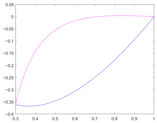
Figure 1 graphically represents the left member of this inequality (blue line) and the right member of this inequality (magenta line) considering the interval of $[0.3,1]$, confirming the validity of the previous inequality. MatlabR2023B software was used throughout this paper.

Now, for Example 5, where $f\left(x\right)={(x-{\displaystyle \frac{1}{2}})}^n$, $ϵ=\delta ={\displaystyle \frac{1}{2}}$ is ${\displaystyle \frac{1}{2}}$-geometric convex on $[1,{\displaystyle \frac{3}{2}}]$ with a modulus of $\mathsf{\Phi }\left(x\right)={\displaystyle \frac{n^2}{2^{2n+1}}}{x}^2$ and $n>0$, the condition from Theorem 4 under the hypothesis that needs to be satisfied is $(x-{\displaystyle \frac{1}{2}})(y-{\displaystyle \frac{1}{2}})=(1-{\displaystyle \frac{1}{2}})({\displaystyle \frac{3}{2}}-{\displaystyle \frac{1}{2}})$. Thus, the inequality from Theorem 4 becomes

$${(x-{\displaystyle \frac{1}{2}})}^n\le {\displaystyle \frac{1}{2^n}}+1-{\displaystyle \frac{1}{{(2x-1)}^n}}-{\displaystyle \frac{n^2}{2^{4n}}}{\displaystyle \frac{ln(x-\frac{1}{2})ln(\frac{1}{2x-1})}{{(ln(2))}^2}}.$$

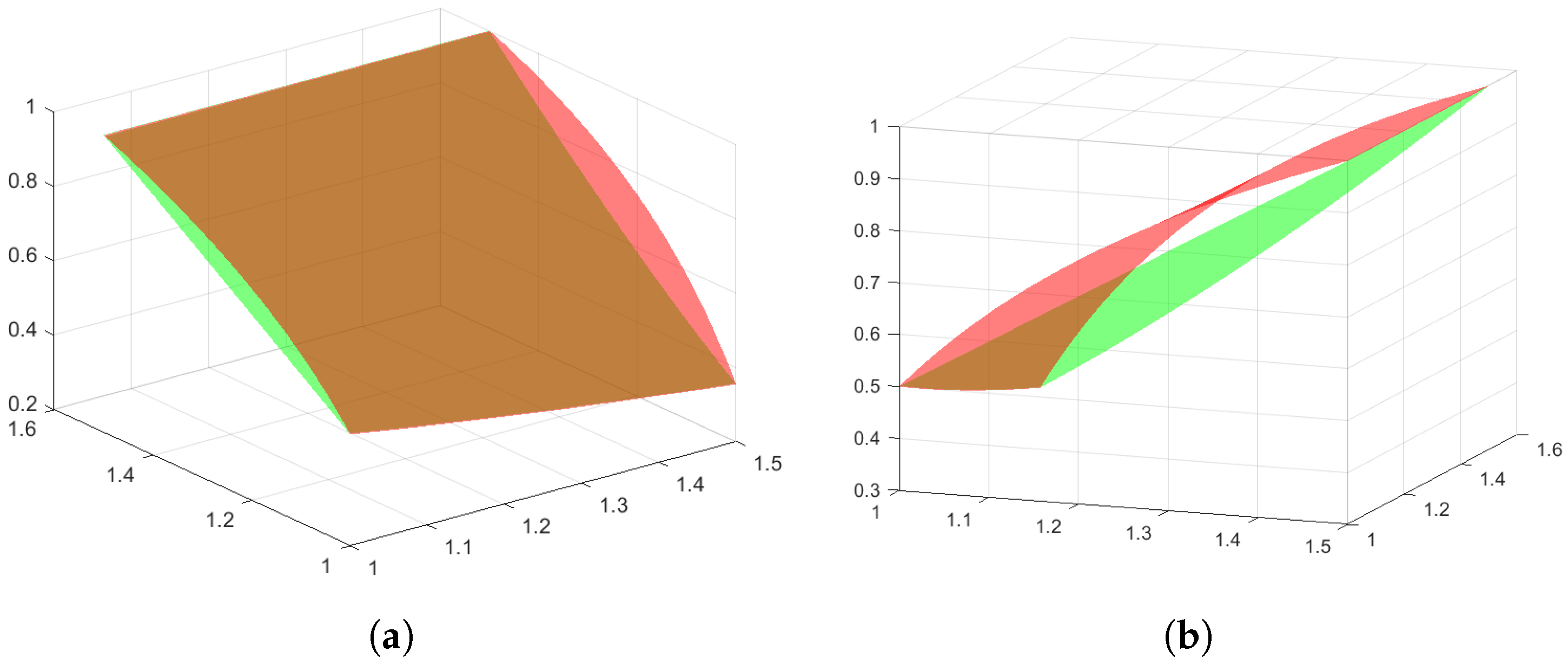
We now consider the same interval $[1,{\displaystyle \frac{3}{2}}]$ for the two variables (x and n) for 3D graphical representations of the left and right members of the previous inequality in order to check the validity of Theorem 4. This graphical representation is presented in Figure 2a. It can be seen that the left member, which is represented as a green surface, is below the right member, which is represented as a red surface. In Figure 2b, the same graphics are given but rotated.

4. Applications to Some Fractional Integrals

In this section, some new integral inequalities are given by using the Caputo–Fabrizio fractional integral operators starting from Theorem 3.

Definition 2

([22,23]). Let $0<\mathsf{\Phi }<\mathsf{\Omega }$ and $F\in H^1(\mathsf{\Phi },\mathsf{\Omega })$ (Sobolev space) for all $\rho \in [0,1],$ where $\beta \left(\rho \right)>0$ is a normalized function with $\beta \left(0\right)=\beta \left(1\right)=1$; then, left and right Caputo–Fabrizio fractional integrals are defined respectively as follows:

$$\left({}_{\mathsf{\Phi }\hspace{0.33em}\hspace{0.33em}}{}^{CF}{I}^{\rho }F\right)\left(z\right)={\displaystyle \frac{1-\rho }{\beta \left(\rho \right)}}F\left(z\right)+{\displaystyle \frac{\rho }{\beta \left(\rho \right)}}{\int }_{\mathsf{\Phi }}^{z}F\left(\gamma \right)d\gamma$$

when $z>\mathsf{\Phi }$ and

$$\left({}^{CF}{I}_{\mathsf{\Omega }}^{\rho }F\right)\left(z\right)={\displaystyle \frac{1-\rho }{\beta \left(\rho \right)}}F\left(z\right)+{\displaystyle \frac{\rho }{\beta \left(\rho \right)}}{\int }_z^{\mathsf{\Omega }}F\left(\gamma \right)d\gamma ,$$

when $z<\mathsf{\Omega }$.

Theorem 7.

Assume that f on $[a,b]$ is a uniformly δ-geometric convex function with modulus ϕ, $0<a<b$, and $f\in H^1(a,b)$ for all $\rho \in [0,1],$ where $\beta \left(\rho \right)>0$ is a normalized function with $\beta \left(0\right)=\beta \left(1\right)=1$; then, we have

$$\left({}_{a\hspace{0.33em}\hspace{0.33em}}{}^{CF}{I}^{\rho }f\right)\left(b\right)\le {\displaystyle \frac{1-\rho }{\beta \left(\rho \right)}}f\left(b\right)+{\displaystyle \frac{\rho }{\beta \left(\rho \right)}}\{f\left(b\right)(b-\delta )-f\left(a\right)(a-\delta )+{\displaystyle \frac{b-a}{ln\left(\frac{a-\delta }{b-\delta }\right)}}[f\left(b\right)-f\left(a\right)]$$

(25)

$$+{\displaystyle \frac{\mathsf{\Phi }(b-a)}{{(ln(\frac{a-\delta }{b-\delta }))}^2}}[2(b-a)+(a+b-2\delta )ln({\displaystyle \frac{a-\delta }{b-\delta }})]\}$$

and

$${\displaystyle \frac{\rho }{\beta \left(\rho \right)}}\{(b-a)f(\sqrt{(a-\delta )(b-\delta )}+\delta )+{\displaystyle \frac{1}{4}}{\int }_a^b\mathsf{\Phi }(u-\delta -{\displaystyle \frac{(a-\delta )(b-\delta )}{u-\delta }})du\}$$

$$\le {\displaystyle \frac{1}{2}}[\left({}_{a\hspace{0.33em}\hspace{0.33em}}{}^{CF}{I}^{\rho }f\right)\left(b\right)-{\displaystyle \frac{1-\rho }{\beta \left(\rho \right)}}f\left(b\right)+{\displaystyle \frac{\rho }{\beta \left(\rho \right)}}{\int }_a^{b}f\left({\displaystyle \frac{(a-\delta )(b-\delta )}{u-\delta }}+\delta \right)du].$$

Proof. 

Here, we consider inequality (3) multiplied by ${(a-\delta )}^t{(b-\delta )}^{1-t}$; then, we integrate the obtained inequality with respect to t over $[0,1]$ and obtain

$$\begin{array}{cc}\hfill & {\int }_0^1{(a-\delta )}^t{(b-\delta )}^{1-t}f({(a-\delta )}^t{(b-\delta )}^{1-t}+\delta )dt\hfill \\ \hfill & \le {\int }_0^1{(a-\delta )}^t{(b-\delta )}^{1-t}[tf\left(a\right)+(1-t)f\left(b\right)-t(1-t)\mathsf{\Phi }(b-a)]dt.\hfill \end{array}$$

By using $v={(a-\delta )}^t{(b-\delta )}^{1-t}+\delta$, we obtain

$$\begin{array}{cc}\hfill & {\int }_a^{b}f\left(v\right)dv\le {\displaystyle \frac{1}{ln\left(\frac{a-\delta }{b-\delta }\right)}}f\left(a\right){\int }_a^{b}ln\left({\displaystyle \frac{v-\delta }{b-\delta }}\right)dv+f\left(b\right){\int }_a^b\left(1-{\displaystyle \frac{ln\left(\frac{v-\delta }{b-\delta }\right)}{ln\left(\frac{a-\delta }{b-\delta }\right)}}\right)dv\hfill \\ \hfill & -\mathsf{\Phi }(b-a){\int }_a^b{\displaystyle \frac{ln\left(\frac{v-\delta }{b-\delta }\right)}{ln\left(\frac{a-\delta }{b-\delta }\right)}}\left(1-{\displaystyle \frac{ln\left(\frac{v-\delta }{b-\delta }\right)}{ln\left(\frac{a-\delta }{b-\delta }\right)}}\right)dv.\hfill \end{array}$$

Now, multiplying the previous expression by ${\displaystyle \frac{\rho }{\beta \left(\rho \right)}}$, by calculus, we get

$$\begin{array}{cc}\hfill & \left({}_{a\hspace{0.33em}\hspace{0.33em}}{}^{CF}{I}^{\rho }f\right)\left(b\right)-{\displaystyle \frac{1-\rho }{\beta \left(\rho \right)}}f\left(b\right)\hfill \\ \hfill & \le {\displaystyle \frac{\rho }{\beta \left(\rho \right)}}\{f\left(a\right){\displaystyle \frac{1}{ln\left(\frac{a-\delta }{b-\delta }\right)}}{\int }_a^{b}ln({\displaystyle \frac{v-\delta }{b-\delta }})dv+f\left(b\right)[(b-a)-{\displaystyle \frac{1}{ln\left(\frac{a-\delta }{b-\delta }\right)}}{\int }_a^{b}ln({\displaystyle \frac{v-\delta }{b-\delta }})dv]\hfill \\ \hfill & -\mathsf{\Phi }(b-a){\displaystyle \frac{1}{{\left(ln\frac{a-\delta }{b-\delta }\right)}^2}}{\int }_a^{b}ln({\displaystyle \frac{v-\delta }{b-\delta }})\left(ln({\displaystyle \frac{a-\delta }{b-\delta }}-ln({\displaystyle \frac{v-\delta }{b-\delta }})\right)dv\},\hfill \end{array}$$

or

$$\begin{array}{cc}\hfill & \left({}_{a\hspace{0.33em}\hspace{0.33em}}{}^{CF}{I}^{\rho }f\right)\left(b\right)-{\displaystyle \frac{1-\rho }{\beta \left(\rho \right)}}f\left(b\right)\le {\displaystyle \frac{\rho }{\beta \left(\rho \right)}}\{f\left(a\right){\displaystyle \frac{1}{ln\left(\frac{a-\delta }{b-\delta }\right)}}I+f\left(b\right)[(b-a)-{\displaystyle \frac{1}{ln\left(\frac{a-\delta }{b-\delta }\right)}}I]\hfill \\ \hfill & -\mathsf{\Phi }(b-a){\displaystyle \frac{1}{{\left(ln\frac{a-\delta }{b-\delta }\right)}^2}}[ln({\displaystyle \frac{a-\delta }{b-\delta }}I-J]\},\hfill \end{array}$$

where $I={\int }_a^{b}ln({\displaystyle \frac{v-\delta }{b-\delta }})dv$ and $J={\int }_a^b{\left(ln({\displaystyle \frac{v-\delta }{b-\delta }})\right)}^{2}dv.$ After calculus, we get the following:

$$\left({}_{a\hspace{0.33em}\hspace{0.33em}}{}^{CF}{I}^{\rho }f\right)\left(b\right)-{\displaystyle \frac{1-\rho }{\beta \left(\rho \right)}}f\left(b\right)\le {\displaystyle \frac{\rho }{\beta \left(\rho \right)}}\{f\left(b\right)(b-\delta )-f\left(a\right)(a-\delta )+{\displaystyle \frac{b-a}{ln\left(\frac{a-\delta }{b-\delta }\right)}}[f\left(b\right)-f\left(a\right)]$$

$$+{\displaystyle \frac{\mathsf{\Phi }(b-a)}{{(ln(\frac{a-\delta }{b-\delta }))}^2}}[2(b-a)+(a+b-2\delta )ln({\displaystyle \frac{a-\delta }{b-\delta }})]\},$$

which gives inequality (25).

For the second inequality, we also take $t={\displaystyle \frac{1}{2}}$ in (3), obtaining

$$f(\sqrt{(x-\delta )(y-\delta )}+\delta )\le {\displaystyle \frac{f\left(x\right)+f\left(y\right)}{2}}-{\displaystyle \frac{1}{4}}\mathsf{\Phi }\left(\right|x-y\left|\right).$$

Now, considering in previous relation, $x={(a-\delta )}^t{(b-\delta )}^{1-t}+\delta$, and $y={(a-\delta )}^{1-t}{(b-\delta )}^t+\delta$, we conclude that

$$\begin{array}{cc}\hfill & f(\sqrt{(a-\delta )(b-\delta )}+\delta )\le {\displaystyle \frac{f({(a-\delta )}^t{(b-\delta )}^{1-t}+\delta )+f({(a-\delta )}^{1-t}{(b-\delta )}^t+\delta )}{2}}\hfill \\ \hfill & -{\displaystyle \frac{1}{4}}{\mathsf{\Phi }\left(\right|(a-\delta )}^t{(b-\delta )}^{1-t}-{(a-\delta )}^{1-t}{(b-\delta )}^t\left|\right),\hfill \end{array}$$

and from here, by multiplication with ${(a-\delta )}^t{(b-\delta )}^{1-t}$ and integration from 0 to 1 with respect to t, we get

$$\begin{array}{cc}\hfill & f(\sqrt{(a-\delta )(b-\delta )}+\delta ){\int }_0^1{(a-\delta )}^t{(b-\delta )}^{1-t}dt\le \hfill \\ \hfill & \le {\int }_0^1{(a-\delta )}^t{(b-\delta )}^{1-t}{\displaystyle \frac{f({(a-\delta )}^t{(b-\delta )}^{1-t}+\delta )+f({(a-\delta )}^{1-t}{(b-\delta )}^t+\delta )}{2}}dt\hfill \\ \hfill & -{\displaystyle \frac{1}{4}}{\int }_0^1{(a-\delta )}^t{(b-\delta )}^{1-t}{\mathsf{\Phi }\left(\right|(a-\delta )}^t{(b-\delta )}^{1-t}-{(a-\delta )}^{1-t}{(b-\delta )}^t\left|\right)dt,\hfill \end{array}$$

After calculus, we find

$$\begin{array}{cc}\hfill & (b-a)f(\sqrt{(a-\delta )(b-\delta )}+\delta )\le \hfill \\ \hfill & \le {\displaystyle \frac{1}{2}}[{\int }_a^{b}f(u)du+{\int }_a^{b}f({\displaystyle \frac{(a-\delta )(b-\delta )}{u-\delta }}+\delta )du]\hfill \\ \hfill & -{\displaystyle \frac{1}{4}}{\int }_a^b\mathsf{\Phi }(|(u-\delta -{\displaystyle \frac{(b-\delta )(a-\delta )}{u-\delta }}|)du,\hfill \end{array}$$

and by multiplication with ${\displaystyle \frac{\rho }{\beta \left(\rho \right)}}$, we obtain

$${\displaystyle \frac{\rho }{\beta \left(\rho \right)}}\{(b-a)f(\sqrt{(a-\delta )(b-\delta )}+\delta )+{\displaystyle \frac{1}{4}}{\int }_a^b\mathsf{\Phi }(u-\delta -{\displaystyle \frac{(a-\delta )(b-\delta )}{u-\delta }})du\}$$

$$\le {\displaystyle \frac{1}{2}}[\left({}_{a\hspace{0.33em}\hspace{0.33em}}{}^{CF}{I}^{\rho }f\right)\left(b\right)-{\displaystyle \frac{1-\rho }{\beta \left(\rho \right)}}f\left(b\right)+{\displaystyle \frac{\rho }{\beta \left(\rho \right)}}{\int }_a^{b}f\left({\displaystyle \frac{(a-\delta )(b-\delta )}{u-\delta }}+\delta \right)du].$$

□

5. Discussion and Conclusions

The aim of this paper is to introduce a new class of convex functions, i.e., the class of uniformly $\delta$-geometric convex functions, and to give novel Jensen–Mercer-type inequalities.

Several nontrivial examples were given in order to underline the difference between previously defined derived classes of geometric convex functions, geometrically–arithmetically convex functions and uniformly convex functions with their variants. The graphic representations presented for these examples also confirm the validity of these results. Such Jensen–Mercer-type inequalities are very important and a main tool in fractional calculus and in finding new error bounds for previously established and published results.

Future research could be conducted to extend these Jensen–Mercer-type inequalities within the framework of interval-valued convex functions.

References

1. Barsam, H.; Sattarzadeh, A.R. Hermite-Hadamard inequalities for uniformly convex functions and its applications in means. Miskolc Math. Notes 2020, 21, 621–830. [Google Scholar] [CrossRef]
2. Barsam, H.; Sayyari, Y. On some inequalities of differentiable uniformly convex mapping with applications. Numer. Funct. Anal. Optim. 2023, 44, 368–381. [Google Scholar] [CrossRef]
3. Dragomir, S.S. Inequalities of Jensen type for HA-convex functions. An. Univ. Oradea Fasc. Mat. 2020, 27, 103–124. [Google Scholar]
4. Işcan, I. Jensen–Mercer inequality for GA-convex functions and some related inequalities. J. Inequal. Appl. 2020, 2020, 212. [Google Scholar] [CrossRef]
5. Niculescu, C.P. Convexity according to the geometric mean. Math. Inequal. Appl. 2000, 3, 155–167. [Google Scholar] [CrossRef]
6. Mercer, A.M. A variant of Jensen’s inequality. J. Inequal. Pure Appl. Math. 2003, 4, 2. [Google Scholar]
7. Niculescu, C.P. Convexity according to means. Math. Inequal. Appl. 2003, 6, 571–580. [Google Scholar] [CrossRef]
8. Noor, M.A.; Noor, K.I.; Awan, M.U. Some inequalities for geometrically-arithmetically h-convex functions. Creat. Math. Inform. 2014, 23, 91–98. [Google Scholar] [CrossRef]
9. Sayyari, Y. A refinement of the Jensen-Simic-Mercer inequality with applications to entropy. J. Korean Soc. Math. Educ. B Pure Appl. Math. 2022, 29, 51–57. [Google Scholar]
10. Valdes, J.E.N.; Rabossi, F.; Samaniego, A.D. Convex functions: Ariadne’s thread or Charlottes’s spiderweb? Adv. Math. Model. Appl. 2020, 5, 176–191. [Google Scholar]
11. Sayyari, Y.; Barsam, H. Jensen-Mercer inequality for uniformly convex functions with some applications. Afr. Mat. 2023, 34, 38. [Google Scholar] [CrossRef]
12. Simic, S. On a global bound for Jensen’s inequality. J. Math. Anal. Appl. 2008, 343, 414–419. [Google Scholar] [CrossRef]
13. Niezgoda, M. A generalization of Mercer’s result on convex functions. Nonlinear Anal. 2009, 71, 2771–2779. [Google Scholar] [CrossRef]
14. Matkovic, A.; Pecaric, J.; Peric, I. A variant of Jensen’s inequality of Mercer type for operators with applications. Linear Algebra Appl. 2006, 418, 551–564. [Google Scholar] [CrossRef]
15. Wang, S.H.; Liu, Q.; Qi, F. On P-geometrically convex sets and functions. J. Appl. Anal. Comput. 2026, 16, 1963–1977. [Google Scholar] [CrossRef]
16. Furuichi, S.; Minculete, N.; Moradi, H.R.; Sababeh, M. Some new properties of geometrically-convex functions. Quaest. Math. 2024, 47, 831–849. [Google Scholar] [CrossRef]
17. Fahad, A.; Wang, Y.; Ali, Z.; Hussain, R.; Furuichi, S. Exploring properties and inequalities for geometrically arithmetically -Cr-convex functions with Cr-order relative entropy. Inf. Sci. 2024, 662, 120219. [Google Scholar] [CrossRef]
18. Sayyari, Y. New entropy bounds via uniformly convex functions. Chaos Solitons Fract. 2020, 141, 110360. [Google Scholar] [CrossRef]
19. Taghavi, A.; Darvish, V.; Azimi, R.T. Hermite-Hadamard type inequalities for operator geometrically convex functions II. Kragujev. J. Math. 2021, 45, 115–125. [Google Scholar] [CrossRef]
20. Hadamard, J. Etude sur les proprietes des founctions entieres et en particulier d’une fonction consideree par Riemann. J. Math. Purees Appl. 1893, 58, 171–215. [Google Scholar]
21. Hermite, C. Sur deux limits d-une integrale definite. Mathesis 1883, 3, 82. [Google Scholar]
22. Munir, A.; Kashuri, A. Analysis On Simpson’s Type Inequalities Through Generalized Convexity with Applications. Sahand Commun. Math. Anal. 2026, 23, 61–83. [Google Scholar]
23. Caputo, M.; Fabrizio, M. On the singular kernels for fractional derivatives. Some applications to partial differential equations. Progr. Fract. Differ. Appl. 2021, 7, 1–4. [Google Scholar]
Figure 1. 2D graphical representation for the left member (blue line) and the right member (magenta line) of the inequality from Theorem 4 in the case of the following function: f ( x ) = x l n ( x ) , δ = 0.02 , a = 0.3 , b = 1 , with Φ ( x ) = 0.02 x 2 on the interval [ 0.3 , 1 ] .
Fractalfract 10 00289 g001
Figure 2. (a) 3D graphical representation for the left member (green surface) and the right member (red surface) of the inequality from Theorem 4 in the case with the following functions and parameters: f ( x ) = ( x 1 2 ) n , ϵ = δ = 1 2 , a = 1 , b = 3 2 , Φ ( x ) = n 2 2 2 n + 1 x 2 , and n [ 1 , 3 2 ] . (b) The same representation as (a) but rotated.
Fractalfract 10 00289 g002
Disclaimer/Publisher’s Note: The statements, opinions and data contained in all publications are solely those of the individual author(s) and contributor(s) and not of MDPI and/or the editor(s). MDPI and/or the editor(s) disclaim responsibility for any injury to people or property resulting from any ideas, methods, instructions or products referred to in the content.