Article

Fractional-Order Typhoid Fever Dynamics and Parameter Identification via Physics-Informed Neural Networks

by
Mallika Arjunan Mani
1,
Kavitha Velusamy
2,
Sowmiya Ramasamy
2 and
Seenith Sivasundaram
3,*
1
Department of Mathematics, School of Arts, Sciences, Humanities and Education, SASTRA Deemed to be University, Thanjavur 613401, Tamil Nadu, India
2
Division of Mathematics and Robotics Engineering, Karunya Institute of Technology and Sciences, Karunya Nagar, Coimbatore 641114, Tamil Nadu, India
3
Department of Mathematics, Bethune-Cookman University, Daytona Beach, FL 32114, USA
*
Author to whom correspondence should be addressed.
Fractal Fract. 2026, 10(4), 270; https://doi.org/10.3390/fractalfract10040270
Submission received: 9 March 2026 / Revised: 14 April 2026 / Accepted: 16 April 2026 / Published: 21 April 2026
(This article belongs to the Special Issue Fractional Dynamics Systems: Modeling, Forecasting, and Control)

Abstract

This paper presents a unified analytical and computational framework for the study of typhoid fever transmission dynamics governed by a Caputo fractional-order compartmental model of order κ ( 0 , 1 ] . The population is stratified into five epidemiological classes, namely susceptible ( S ) , asymptomatic ( A ) , symptomatic ( I ) , hospitalised ( H ) , and recovered ( R ) , and the governing system explicitly incorporates asymptomatic transmission, treatment dynamics, and temporary immunity with waning. The use of the Caputo fractional derivative is motivated by the well-documented existence of chronic asymptomatic Salmonella Typhi carriers, whose heavy-tailed sojourn times in the carrier state are naturally encoded by the Mittag–Leffler waiting-time distribution arising from the fractional operator. A complete qualitative analysis of the fractional system is carried out: the basic reproduction number R 0 is derived via the next-generation matrix method; local and global asymptotic stability of both the disease-free equilibrium E 0 (when R 0 1 ) and the endemic equilibrium E * (when R 0 > 1 ) are established using fractional Lyapunov theory and the LaSalle invariance principle; and the normalised sensitivity indices of R 0 are computed to identify transmission-amplifying and transmission-suppressing parameters. Existence, uniqueness, and Ulam–Hyers stability of solutions are established via Banach and Leray–Schauder fixed-point arguments. To complement the analytical results, a fractional physics-informed neural network ( PINN ) framework is developed to simultaneously reconstruct compartmental trajectories and identify unknown biological parameters from sparse synthetic observations. PINN embeds the L1-Caputo discretisation directly into the training residuals and employs a four-stage Adam–L-BFGS optimisation strategy to recover five trainable parameters Θ = { ϕ , μ , σ , ψ , β } across three fractional orders κ { 1.0 , 0.95 , 0.9 } . The estimated parameters show strong agreement with the true values at the classical limit κ = 1.0 ( MAPE = 2.27 % ), with the natural mortality rate μ recovered with APE 0.51 % and the transmission rate β with APE 3.63 % across all fractional orders, confirming the structural identifiability of the model. Pairwise correlation analysis of the learned parameters establishes the absence of equifinality, validating that β can be reliably included in the trainable set. Noise robustness experiments under Gaussian perturbations of 1 % , 3 % , and 5 % demonstrate graceful degradation ( MAPE : 0.82 % 3.10 % 7.31 % ), confirming the reliability of the proposed framework under realistic observational conditions.

1. Introduction

Typhoid fever, caused by the bacterium Salmonella enterica serovar Typhi, continues to impose a substantial public health burden in low- and middle-income countries, with an estimated 11–21 million new cases and 128,000 –161,000 deaths reported annually worldwide [1]. Despite the availability of effective vaccines and antibiotic therapies, the disease persists endemically across sub-Saharan Africa and South Asia, driven primarily by inadequate access to safe water, poor sanitation infrastructure, and the under-recognised role of asymptomatic carriers in sustaining community-level transmission [2,3]. A distinctive epidemiological feature of typhoid is the existence of asymptomatic carriers, that is, individuals who harbour and shed the pathogen without manifesting clinical symptoms, which substantially complicates detection, surveillance, and control efforts [4]. Mathematical modelling has therefore become an indispensable tool for elucidating the interplay between these transmission pathways, quantifying epidemiological thresholds, and evaluating the population-level impact of therapeutic and preventive interventions [5,6].
Classical integer-order compartmental models, built upon the assumption of instantaneous state transitions, have provided valuable insights into typhoid dynamics [7,8]. However, biological processes such as incubation variability, gradual immunity waning, and heterogeneous treatment response are inherently history-dependent: the current rate of change in each epidemiological compartment depends not only on the present state of the system but also on its entire past trajectory. Standard ordinary differential equation frameworks are structurally incapable of encoding such non-Markovian, long-memory effects [9]. Fractional calculus, and in particular the Caputo fractional derivative, offers a mathematically rigorous and biologically motivated remedy: by replacing the integer-order derivative d / d ς with the Caputo operator D ς κ C of order κ ( 0 , 1 ] , the governing equations acquire a convolution structure that naturally captures power-law memory and hereditary effects characteristic of subdiffusive biological dynamics [10,11]. Crucially, the use of fractional-order derivatives in the present typhoid model is not a generic mathematical generalisation chosen for analytical convenience. The Caputo fractional structure of system (10) is the exact population-level consequence of a specific, biologically documented, and mathematically falsifiable assumption: the sojourn-time distribution of chronic asymptomatic Salmonella Typhi carriers follows a Mittag–Leffler law rather than an exponential law. This derivation follows the rigorous continuous-time random walk (CTRW) framework of Angstmann et al. [12], who proved that Mittag–Leffler-distributed sojourn times in a compartment yield, in the population-level mean-field limit, exactly a Caputo fractional differential equation governing that compartment, not as an approximation but as an identity. The biological motivation is precise: approximately 2 to 5% of typhoid-infected individuals develop long-term gallbladder colonisation and continue to shed the pathogen for months, years, or even decades after clinical recovery [2,4]. The exponential survival function, which is the structural assumption of every integer-order compartmental model, requires the probability of remaining asymptomatic beyond time ς to decay as e ( α + μ ) ς , a property fundamentally incompatible with empirically documented power-law carrier persistence. Replacing it with the Mittag–Leffler survival function
φ A ( ς ) = E κ , 1 ( α κ + μ κ ) ς κ , κ ( 0 , 1 ] ,
which has power-law tail φ A ( ς ) ς κ / [ ( α κ + μ κ ) Γ ( 1 κ ) ] for large ς and reduces to the exponential at κ = 1 , the CTRW master equation for the asymptomatic compartment yields, upon taking the population-level limit, precisely the second equation of system (10) (see Section 2.2). The fractional order κ is therefore not a fitting parameter but the tail exponent of the empirical chronic carrier sojourn-time distribution, a directly falsifiable quantity that the PINN framework of Section 5 provides to a computational pathway to estimate from aggregate compartmental data. When κ = 1 , the Mittag–Leffler survival function reduces to the exponential, and system (10) recovers the classical integer-order typhoid model exactly; the fractional model therefore subsumes the standard framework as a strict limiting case.
The application of fractional calculus to epidemic modelling has expanded rapidly over the past decade. Fractional extensions of the classical SIR and SEIR frameworks have been analysed for diseases including HIV [13,14], tuberculosis [15], COVID-19 [16], and malaria [17], consistently demonstrating that fractional-order models provide a more accurate and flexible fit to observed epidemic trajectories than their integer-order counterparts. For typhoid fever specifically, ref. [18] recently analysed a fractional typhoid model with optimal control, whilst ref. [19] investigated numerical solution strategies via generalised fractional Adams–Bashforth–Moulton methods. These studies confirm the epidemiological relevance of fractional-order modelling for typhoid, yet a complete analytical treatment encompassing existence and uniqueness, Ulam–Hyers stability, global Lyapunov stability of both equilibria, and sensitivity analysis within a unified framework remains an open contribution.
A complementary and increasingly prominent challenge in epidemic modelling is the inverse problem: given observed compartmental data, how can one reliably estimate the underlying biological parameters that govern transmission, recovery, and immunity dynamics? Classical approaches such as least-squares fitting, Bayesian inference, and nonlinear optimisation are computationally intensive, often require full state observability, and do not natively enforce the governing differential equations as hard constraints on the estimated trajectories [20]. To address this limitation, ref. [21] introduced PINN s, which incorporate the residuals of the governing equations into the network’s loss function, a technique now widely adopted in scientific computing. The resulting framework simultaneously learns a surrogate solution to the forward problem and identifies unknown parameters from sparse, potentially noisy observations, with the governing physics acting as a regulariser that prevents over-fitting and enforces biological consistency of the learned trajectories [22].
The extension of PINN methodology to fractional differential equations presents additional mathematical challenges: the Caputo operator is nonlocal and its evaluation via automatic differentiation is not straightforward. Ref. [23] recently demonstrated that fractional memory effects in epidemic models can be identified from data using PINN s applied to a fractional SEIRD system, and ref. [16] proposed a PINN framework for fractional COVID-19 modelling with simultaneous order estimation. Ref. [24] established identifiability and predictability results for both integer- and fractional-order epidemic PINN s, providing a theoretical foundation for the use of such methods in parameter inference. Nevertheless, the application of fractional PINN frameworks to typhoid fever, with its distinctive asymptomatic transmission structure and temporary immunity mechanism, has not yet been investigated.
Motivated by these gaps, the present paper makes the following contributions:
1.
We formulate a Caputo fractional-order SAIHR compartmental model for typhoid fever incorporating asymptomatic transmission, treatment dynamics, and temporary immunity with waning. The Caputo structure is derived from the stochastic sojourn-time dynamics of chronic Salmonella Typhi carriers via a CTRW argument: when the survival function of the asymptomatic compartment follows the Mittag–Leffler law E κ , 1 ( ( α κ + μ κ ) ς κ ) , the population-level mean-field equation is exactly the Caputo fractional Equation (9), with the fractional order  κ identified as the tail exponent of the empirical carrier sojourn-time distribution (Section 2.2, Remark 1).
2.
We carry out a complete qualitative analysis of the model: the basic reproduction number R 0 is derived via the next-generation matrix method [25]; the disease-free equilibrium E 0 is shown to be globally asymptotically stable when R 0 1 ; and the endemic equilibrium E * is shown to be globally asymptotically stable when R 0 > 1 , using fractional Lyapunov functions and the LaSalle invariance principle [26].
3.
Existence and uniqueness of solutions are established via Banach and Picard fixed-point arguments and the Leray–Schauder theorem, and Ulam–Hyers stability is proved to quantify the structural robustness of the fractional system against bounded perturbations.
4.
A fractional PINN framework is developed that embeds the L1-Caputo discretisation [23] directly into the training residuals and employs a four-stage Adam–L-BFGS multi-optimiser strategy to simultaneously reconstruct all five compartmental trajectories and identify four unknown biological parameters Θ = { ϕ , μ , σ , ψ , β } from sparse observations across fractional orders κ { 1.0 , 0.95 , 0.9 } .
5.
The framework achieves MAPE = 2.27 % at the classical limit κ = 1.0 , with the natural mortality rate μ recovered to within 0.51 % and the transmission rate β to within 3.63 % across all fractional orders. Pairwise correlation analysis confirms the absence of parameter equifinality, and noise robustness experiments under Gaussian perturbations of 1 % , 3 % , and 5 % demonstrate graceful degradation ( MAPE : 0.82 % 3.10 % 7.31 % ), validating both the structural identifiability of the model and the reliability of the proposed optimisation strategy.
The remainder of the paper is organised as follows. Section 2 formulates the fractional compartmental model and provides a detailed biological description of all parameters. Section 3 presents the mathematical preliminaries, including the non-negativity and boundedness of solutions, equilibrium analysis, stability theory, sensitivity analysis, and existence–uniqueness results. Section 4 presents numerical simulations illustrating the role of the fractional order κ and key epidemiological parameters. Section 5 develops the fractional PINN framework, covering the network architecture, L1 discretisation, composite loss function, parameter estimation strategy, and multi-stage optimisation algorithm. Section 6 presents and discusses the computational results. Section 7 summarises the findings and outlines directions for future work.

2. Mathematical Model

Typhoid fever remains a significant public health burden globally [5,6]. Mathematical modelling provides a systematic framework to quantify transmission pathways, evaluate intervention strategies, and estimate key epidemiological thresholds such as R 0 . In what follows, we formulate a Caputo fractional-order compartmental model that explicitly accounts for asymptomatic transmission, treatment dynamics, and temporary immunity.

2.1. Model Formulation

The total human population at time ς is partitioned into five mutually exclusive and collectively exhaustive epidemiological compartments [7]:
  • S ( ς ) : individuals who are susceptible to infection;
  • A ( ς ) : individuals who are infected but asymptomatic (subclinical carriers);
  • I ( ς ) : individuals who are symptomatically infected;
  • H ( ς ) : individuals who are currently undergoing treatment;
  • R ( ς ) : individuals who have recovered and acquired temporary immunity.

2.2. From Chronic Carrier Biology to Fractional Dynamics: A CTRW Derivation

The Caputo fractional structure of system (10) is derived here from the stochastic dynamics of individual chronic Salmonella Typhi carriers, following the CTRW framework of Angstmann et al. [12]. The derivation establishes that the fractional operator is a mathematical consequence of a specific biological assumption, not a modelling choice.
  • Step 1: Individual-level stochastic process.
Consider an individual who enters the asymptomatic compartment A at time ς 0 . Let T A denote their random sojourn time in A before either progressing to symptomatic infection or dying. In the classical integer-order model, T A is exponentially distributed with rate ( α + μ ) , yielding the survival function
φ A cl ( ς ) = Pr T A > ς = e ( α + μ ) ς , ς 0 .
This exponential form is the precise expression of the Markovian (memoryless) hypothesis: the probability of leaving compartment A in the next instant depends only on the current state, not on how long the individual has already been asymptomatic.
  • Step 2: Biological falsification of the exponential assumption for typhoid.
The Markovian hypothesis is structurally inconsistent with the chronic carrier biology of Salmonella Typhi. Approximately 2 to 5% of typhoid-infected individuals remain asymptomatic carriers and continue to shed the pathogen for months, years, or even decades after clinical recovery [2,4]. If carrier persistence were governed by (1), the probability of remaining asymptomatic beyond ς = 365 days would be e ( α + μ ) × 365 e 11 10 5 using the base parameter values of Table 1, which is four orders of magnitude below the observed 2 to 5% chronic carrier prevalence. The exponential survival function (1) is therefore quantitatively incompatible with the typhoid carrier literature.
  • Step 3: The Mittag–Leffler survival function as the mechanistic replacement.
We replace the exponential survival function with the one-parameter Mittag–Leffler form
φ A ( ς ) = E κ , 1 ( α κ + μ κ ) ς κ , κ ( 0 , 1 ] ,
where E κ , 1 ( z ) = j = 0 z j / Γ ( κ j + 1 ) . The corresponding waiting-time density is
ψ A ( ς ) = d d ς φ A ( ς ) = ( α κ + μ κ ) ς κ 1 E κ , κ ( α κ + μ κ ) ς κ ,
which exhibits the power-law tail
ψ A ( ς ) ς 1 κ ( α κ + μ κ ) Γ ( 1 κ ) as ς ,
encoding the heavy-tailed carrier persistence observed empirically. For κ = 1 , the function (2) reduces exactly to e ( α + μ ) ς , recovering the classical model as a limiting case.
Remark 1 (Biological interpretation of κ ).
The fractional order κ in (2) is not a free fitting parameter; it is the tail exponent of the empirical chronic carrier sojourn-time distribution. A smaller value of κ corresponds to a heavier power-law tail, representing a population in which a larger fraction of asymptomatic individuals remain infectious for exceptionally long durations. The value κ = 1 recovers the Markovian limit with exponentially distributed sojourn times, while κ < 1 progressively models populations with increasing chronic carrier burden. This interpretation is directly falsifiable from longitudinal carrier cohort studies, and the PINN framework of Section 5 provides a computational pathway to estimate κ from aggregate compartmental observations.
  • Step 4: Population-level Caputo equation via CTRW.
Let q + ( A , ς ) = β κ S ( ς ) I ( ς ) denote the flux of newly infected asymptomatic individuals entering A at time ς . The number of individuals in A at time ς is given by
A ( ς ) = 0 ς φ A ( ς ς 0 ) q + ( A , ς 0 ) d ς 0 + A 0 ( ς ) ,
where A 0 ( ς ) accounts for individuals already asymptomatic at time 0. Differentiating (5) and eliminating q + via Laplace convolution, the master equation for A takes the form
d A ( ς ) d ς = q + ( A , ς ) 0 ς K A ( ς ς 0 ) A ( ς 0 ) d ς 0 μ κ A ( ς ) ,
where the memory kernel K A satisfies
L { K A } ( s ) = L { ψ A } ( s ) L { φ A } ( s ) = s 1 κ ( α κ + μ κ ) .
Taking the Laplace transform of (6) and applying the standard Caputo transform formula L { D ς κ C A ( ς ) } ( s ) = s κ A ˜ ( s ) s κ 1 A ( 0 ) with the kernel identity (7), the transformed equation reads
s κ A ˜ ( s ) s κ 1 A 0 = β κ S I ˜ ( s ) α κ + μ κ A ˜ ( s ) .
Inverting (8) directly yields
D ς κ C A ( ς ) = β κ S ( ς ) I ( ς ) α κ + μ κ A ( ς ) ,
which is precisely the second equation of system (10). The Caputo fractional structure follows directly from the Mittag–Leffler sojourn-time assumption (2), with the prescribed initial condition A ( 0 ) = A 0 entering naturally through the Caputo transform formula.
  • Step 5: Extension to the full SAIHR system.
The same CTRW argument applies to each compartment of system (10). Each transition is governed by a Mittag–Leffler survival function with tail exponent κ , and the resulting memory kernels all yield the Laplace-domain signature (7). The fractional order κ therefore encodes a single systemic population-level property: the prevalence and duration of chronic asymptomatic carriage propagating through the full transmission cycle S A I H R S . The full system (10) is thus the exact mean-field limit of a CTRW through the five SAIHR compartments under Mittag–Leffler sojourn times, and the p κ scaling of all rate parameters follows directly from dimensional consistency of this derivation (Remark 2).
With the preceding CTRW derivation having established the mechanistic basis for the Caputo structure, the full fractional-order compartmental model is now stated. The total living population is N ( ς ) = S ( ς ) + A ( ς ) + I ( ς ) + H ( ς ) + R ( ς ) , and the governing system of Caputo fractional differential equations of order κ ( 0 , 1 ] , constructed by balancing the inflow and outflow of individuals in each epidemiological class, is
D ς κ C S ( ς ) = Ω κ + ϕ κ R ( ς ) β κ S ( ς ) I ( ς ) μ κ S ( ς ) , D ς κ C A ( ς ) = β κ S ( ς ) I ( ς ) α κ + μ κ A ( ς ) , D ς κ C I ( ς ) = α κ A ( ς ) ψ κ + δ κ + μ κ I ( ς ) , D ς κ C H ( ς ) = ψ κ I ( ς ) σ κ + δ κ + μ κ H ( ς ) , D ς κ C R ( ς ) = σ κ H ( ς ) ϕ κ + μ κ R ( ς ) ,
subject to non-negative initial conditions
S ( 0 ) = S 0 , A ( 0 ) = A 0 , I ( 0 ) = I 0 , H ( 0 ) = H 0 , R ( 0 ) = R 0 , S 0 , A 0 , I 0 , H 0 , R 0 0 .
Remark 2 (Dimensional consistency).
The Caputo fractional derivative D ς κ C carries units [ time ] κ , so the left-hand side of each equation in (10) has units [ population ] · [ time ] κ . For the right-hand side to be dimensionally homogeneous, every rate parameter p with classical unit [ time ] 1 must be replaced by p κ , which carries unit [ time ] κ . This substitution is standard in fractional epidemic modelling [15] and leaves the biological interpretation of each parameter unchanged. When κ = 1 , all powers reduce to unity and system (10) recovers the classical integer-order typhoid model exactly.
We note that the recruitment rate Ω has classical unit [ population · time 1 ] . In the fractional setting, Ω is interpreted as having been non-dimensionalised with respect to a reference population N ref , so that its effective unit is [ time 1 ] ; the substitution Ω Ω κ then produces the correct unit [ time κ ] on the right-hand side. Equivalently, one may regard all state variables as dimensionless fractions of N ref , in which case every parameter in system (10) carries unit [ time 1 ] and the p κ substitution is uniformly valid.

2.3. Biological Description of Parameters

Each parameter in system (10) governs a specific and biologically interpretable mechanism. The κ -th power of each rate parameter arises solely from dimensional consistency and does not alter the underlying biological meaning; the descriptions below therefore refer to the base (integer-order) parameters.

2.3.1. Susceptible Compartment S ( ς )

The susceptible population evolves according to the first equation of (10). The parameter Ω > 0 represents the constant recruitment of new individuals into the susceptible class through birth or immigration; its κ -th power Ω κ provides a dimensionally consistent source term. The term ϕ κ R ( ς ) denotes the waning of immunity among recovered individuals, who return to susceptibility at rate ϕ > 0 . Infection occurs through effective contact between susceptible and symptomatic individuals at transmission rate β > 0 , captured by the bilinear incidence term β κ S ( ς ) I ( ς ) . Natural mortality of susceptible individuals occurs at rate μ κ .

2.3.2. AsymptomaticInfected Compartment A ( ς )

The asymptomatic class satisfies the second equation of (10). The inflow β κ S ( ς ) I ( ς ) describes newly infected individuals who do not yet manifest clinical symptoms; such asymptomatic carriers sustain undetected community transmission. The parameter α > 0 describes the progression rate from asymptomatic to symptomatic infection, reflecting clinical disease developments, and the combined outflow rate is ( α κ + μ κ ) .

2.3.3. SymptomaticInfected Compartment I ( ς )

The symptomatic infected population is governed by the third equation of (10). The inflow α κ A ( ς ) captures disease progression from the asymptomatic stage. The parameter ψ > 0 represents the rate at which symptomatic individuals initiate treatment and enter the treated class H . The disease-induced mortality rate δ > 0 accounts for deaths directly attributable to active infection, and the total outflow rate is ( ψ κ + δ κ + μ κ ) .

2.3.4. TreatedCompartment H ( ς )

The treated population evolves according to the fourth equation of (10). Individuals enter treatment from the symptomatic class at rate ψ κ . Successful recovery from treatment occurs at rate σ κ , transferring individuals to the recovered class R . Disease-related mortality persists during treatment at rate δ κ , giving a total outflow rate of ( σ κ + δ κ + μ κ ) .

2.3.5. RecoveredCompartment R ( ς )

The recovered class is described by the fifth equation of (10). Inflow arises from successful treatments at rate σ κ H ( ς ) . Since immunity to typhoid is temporary, individuals lose protection at rate ϕ κ , returning to the susceptible class. The total outflow rate is ( ϕ κ + μ κ ) .

2.3.6. Population-Level Flow

The structured interaction of these parameters generates the cyclic disease progression
S β κ S I A α κ I ψ κ H σ κ R ϕ κ S ,
while mortality ( μ κ from all compartments; δ κ additionally from I and H ) acts as an outflow across multiple compartments. This parameter-driven flow ensures biological feasibility and provides the foundation for the subsequent analytical and computational investigations.

2.4. Parameter Summary

Table 1 summarises all parameters appearing in system (10), together with their biological interpretation and base values used in numerical experiments.

3. Preliminaries

In this section, we present the fundamental concepts of the Caputo fractional derivative, which have gained significant attention in recent years due to their ability to model complex systems with memory effects.
Definition 1 
(Caputo fractional derivative [9]). The Caputo fractional derivative of order 0 < κ < 1 for z ( ς ) , where m 1 κ m , m N , is described as
( D 0 + κ C z ) ( ς ) = 1 Γ ( m κ ) 0 ς ( ς τ ) m κ 1 z m ( τ ) d τ .
Definition 2 
(Riemann–Liouville fractional integral [9]). For κ > 0 , the Riemann–Liouville fractional integral of order κ of a function z ( ς ) is
( I 0 + κ z ) ( ς ) = 1 Γ ( κ ) 0 ς ( ς τ ) κ 1 z ( τ ) d τ .
Theorem 1 
([27]). Let 0 < κ 1 , Z > 0 , and consider the Caputo fractional initial-value problem
( D 0 + κ C y ) ( ς ) = f ( ς , y ( ς ) ) , ς ( 0 , Z ) , y ( 0 ) = y 0 .
Suppose f : [ 0 , Z ] × R R is continuous in ς and locally Lipschitz in y, and y is continuous on [ 0 , Z ] with Caputo derivative on ( 0 , Z ) . Then, y solves (14) if and only if
y ( ς ) = y 0 + I 0 + κ ( f ( · , y ( · ) ) ) ( ς ) ,
where I 0 + κ denotes the Riemann–Liouville fractional integral of order κ.
Proof. 
(⇒) If y solves (14), applying I 0 + κ to both sides and using the identity I 0 + κ D 0 + κ C y ( ς ) = y ( ς ) y ( 0 ) give y ( ς ) y 0 = I 0 + κ ( f ( · , y ( · ) ) ) ( ς ) , which is (15).
(⇐) If y satisfies (15), then f ( s , y ( s ) ) is continuous on [ 0 , Z ] , so the right-hand side is continuous. Applying D 0 + κ C to (15) yields D 0 + κ C y ( ς ) = D 0 + κ C I 0 + κ ( f ( · , y ( · ) ) ) ( ς ) = f ( ς , y ( ς ) ) , and clearly, y ( 0 ) = y 0 , establishing (14).    □
Lemma 1 
([28]). Suppose κ ( 0 , 1 ) , ς 0 0 , and X : [ ς 0 , ) R + is a continuous positive function. Then, for every constant X * R + and all ς ς 0 ,
D ς κ C X ( ς ) X * X * ln X ( ς ) X * 1 X * X ( ς ) D ς κ C X ( ς ) ,
where D ς κ C is the Caputo fractional derivative of order κ with lower limit ς 0 .
Lemma 2.
Consider the linear Caputo fractional differential equation governing the total population N ( ς ) = S ( ς ) + A ( ς ) + I ( ς ) + H ( ς ) + R ( ς ) of system (10), namely
D ς κ C N ( ς ) = Ω κ μ κ N ( ς ) , N ( 0 ) = N 0 , κ ( 0 , 1 ] .
Then, the unique solution of (17) is
N ( ς ) = Ω κ μ κ + N 0 Ω κ μ κ E κ μ κ ς κ ,
where E κ ( · ) denotes the one-parameter Mittag–Leffler function. Moreover,
lim ς N ( ς ) = Ω κ μ κ .
Proof. 
Recall that the one-parameter Mittag–Leffler function is defined by the entire series
E κ ( z ) = j = 0 z j Γ ( κ j + 1 ) , z C , κ > 0 ,
which converges absolutely for all z C . For κ = 1 , E 1 ( z ) = e z , recovering the classical exponential. The asymptotic behaviour for κ ( 0 , 1 ) and real λ > 0 is
E κ ( λ ς κ ) ς κ λ Γ ( 1 κ ) 0 as ς ,
confirming the algebraic (power-law) decay characteristic of fractional relaxation.
Applying the Laplace transform L { · } ( s ) to both sides of (17) and invoking the standard Caputo transform formula
L D ς κ C N ( ς ) ( s ) = s κ N ˜ ( s ) s κ 1 N ( 0 ) ,
where N ˜ ( s ) = L { N ( ς ) } ( s ) , we obtain
s κ N ˜ ( s ) s κ 1 N 0 = Ω κ s μ κ N ˜ ( s ) .
Collecting the terms involving N ˜ ( s ) on the left-hand side of (23) gives
N ˜ ( s ) s κ + μ κ = Ω κ s + s κ 1 N 0 ,
and hence,
N ˜ ( s ) = Ω κ s s κ + μ κ + s κ 1 N 0 s κ + μ κ .
The two inverse Laplace pairs associated with E κ are
L 1 s κ 1 s κ + μ κ ( ς ) = E κ μ κ ς κ ,
L 1 1 s s κ + μ κ ( ς ) = 1 μ κ 1 E κ μ κ ς κ .
Applying (26)–(27) to (25) yields
N ( ς ) = Ω κ μ κ 1 E κ μ κ ς κ + N 0 E κ μ κ ς κ .
That is,
N ( ς ) = Ω κ μ κ + N 0 Ω κ μ κ E κ μ κ ς κ ,
establishing (18). By the asymptotic decay property (21), E κ ( μ κ ς κ ) 0 as ς for all κ ( 0 , 1 ) , and for κ = 1 , the same follows from e μ ς 0 . Therefore,
lim ς N ( ς ) = Ω κ μ κ + N 0 Ω κ μ κ · 0 = Ω κ μ κ ,
which establishes (19) and completes the proof.    □

3.1. Non-Negativity and Boundedness

Since the model (10) represents human populations, it is necessary to prove that all the state variables are non-negative ς 0 .
Theorem 2 (Positively invariant region).
Let N ( ς ) = S ( ς ) + A ( ς ) + I ( ς ) + H ( ς ) + R ( ς ) denote the total population of the fractional typhoid system (10) with non-negative initial conditions (11). Then, the closed region
Ξ = S , A , I , H , R R + 5 : 0 N ( ς ) Ω κ μ κ
is positively invariant and attractive with respect to system (10) for all ς 0 .
Proof. 
Summing all five equations of system (10) and noting that disease-induced mortality removes individuals from I ( ς ) and H ( ς ) , the total population satisfies
D ς κ C N ( ς ) = Ω κ μ κ N ( ς ) δ κ I ( ς ) + H ( ς ) Ω κ μ κ N ( ς ) ,
since I ( ς ) , H ( ς ) 0 for all ς 0 . Introducing the comparison variable Y ( ς ) governed by the equality case of (32) with Y ( 0 ) = N 0 , Lemma 2 supplies its explicit Mittag–Leffler solution
Y ( ς ) = Ω κ μ κ + N 0 Ω κ μ κ E κ μ κ ς κ .
Since E κ ( μ κ ς κ ) [ 0 , 1 ] for all ς 0 and κ ( 0 , 1 ] , the expression (33) represents a convex interpolation between N 0 and Ω κ / μ κ when N 0 Ω κ / μ κ and decreases monotonically toward Ω κ / μ κ from above otherwise, owing to the algebraic decay E κ ( μ κ ς κ ) 0 as ς established in (21). In either case,
0 Y ( ς ) Ω κ μ κ , ς 0 .
Applying the fractional comparison principle [27] to (32) with N ( 0 ) = Y ( 0 ) gives N ( ς ) Y ( ς ) , and combining this with N ( ς ) 0 , which follows from the non-negativity of all state variables under initial conditions (11), we conclude
0 N ( ς ) Y ( ς ) Ω κ μ κ , ς 0 .
The bound (35) guarantees that any trajectory initiating in Ξ remains there for all future times, establishing positive invariance. Since Y ( ς ) Ω κ / μ κ as ς by Lemma 2, every solution originating outside Ξ is eventually drawn into and confined within Ξ , confirming that Ξ is attractive. We emphasise that the bound N ( ς ) Ω κ / μ κ is not tight whenever I ( ς ) or H ( ς ) is positive, since the disease-induced mortality term δ κ ( I + H ) 0 was dropped when deriving inequality (32). The true equilibrium total population satisfies
N * = Ω κ μ κ + δ κ ( I * + H * ) / N * < Ω κ μ κ ,
so that Ω κ / μ κ serves as a conservative upper bound rather than the exact equilibrium population. Consequently, system (10) is epidemiologically well-posed and all subsequent analysis is conducted within Ξ .    □
Theorem 3 (Non-negativity of solutions).
Let the initial conditions satisfy (11). Then, every solution S ( ς ) , A ( ς ) , I ( ς ) , H ( ς ) , R ( ς ) of system (10) remains non-negative for all ς 0 , that is,
S ( ς ) , A ( ς ) , I ( ς ) , H ( ς ) , R ( ς ) 0 , ς 0 .
Proof. 
We establish non-negativity for S ( ς ) in detail; the remaining compartments follow by an identical argument, summarised at the end.
Since R ( ς ) 0 and all parameters are positive, the first equation of system (10) satisfies the differential inequality
D ς κ C S ( ς ) = Ω κ + ϕ κ R ( ς ) β κ S ( ς ) I ( ς ) μ κ S ( ς ) β κ I ( ς ) + μ κ S ( ς ) .
As a direct consequence of Theorem 2, all solutions are confined to Ξ , and therefore, the susceptible population is uniformly bounded, so there exists a finite constant a = β κ M + μ κ > 0 , where M = sup ς 0 I ( ς ) < , such that (36) reduces to
D ς κ C S ( ς ) a S ( ς ) .
Applying the Laplace transform to (37) with the Caputo formula (22) and denoting S ^ ( s ) = L { S ( ς ) } ( s ) gives
s κ S ^ ( s ) s κ 1 S 0 a S ^ ( s ) ,
which rearranges to
S ^ ( s ) S 0 s κ 1 s κ + a .
Inverting via the Mittag–Leffler pair (26) yields
S ( ς ) S 0 E κ a ς κ 0 , ς 0 ,
since S 0 0 and E κ ( a ς κ ) ( 0 , 1 ] for all ς 0 , κ ( 0 , 1 ] , and a > 0 .
Applying the same reasoning to the remaining four equations of (10) and invoking the Laplace–Mittag–Leffler argument above delivers
A ( ς ) A 0 E κ ( K 1 ς κ ) 0 , I ( ς ) I 0 E κ ( K 2 ς κ ) 0 ,
H ( ς ) H 0 E κ ( K 3 ς κ ) 0 , R ( ς ) R 0 E κ ( K 4 ς κ ) 0 .
Here, K 1 K 4 , as defined in (40), denote the total outflow rates from the respective compartments in system (10). Hence, all state variables remain non-negative for all ς 0 , and the biologically feasible region Ξ defined in (31) is forward-invariant under system (10).    □

3.2. Analysis of Equilibrium Points, Reproduction Number, and Stability

We now carry out a complete qualitative analysis of system (10), comprising the computation of equilibrium points, the derivation of the basic reproduction number via the next-generation matrix method, and the investigation of local and global stability of both the disease-free and endemic equilibria.

3.2.1. Disease-Free Equilibrium

The disease-free equilibrium (DFE) corresponds to the state in which the infection is entirely absent from the population. Setting all infected compartments to zero, i.e., A = I = H = 0 , and solving the remaining equations of (10) at steady state yields the unique DFE
E 0 = Ω κ μ κ , 0 , 0 , 0 , 0 .
The positive quantity Ω κ / μ κ represents the equilibrium susceptible population sustained by recruitment alone in the absence of infection.

3.2.2. Basic Reproduction Number

The basic reproduction number R 0 is derived using the next-generation matrix (NGM) method of [25]. The infected compartments of system (10) are A ( ς ) and I ( ς ) . Decomposing their right-hand sides into new infection terms F and transition terms V gives
F = β κ S I 0 , V = ( α κ + μ κ ) A ( ψ κ + δ κ + μ κ ) I α κ A .
For notational compactness, define the composite outflow rates
K 1 = α κ + μ κ , K 2 = ψ κ + δ κ + μ κ , K 3 = σ κ + δ κ + μ κ , K 4 = ϕ κ + μ κ .
Evaluating the Jacobians of F and V at the DFE E 0 yields
F = 0 β κ Ω κ μ κ 0 0 , V = K 1 0 α κ K 2 ,
with inverse
V 1 = 1 K 1 K 2 K 2 0 α κ K 1 .
We note that V is a non-singular M-matrix: its diagonal entries K 1 , K 2 > 0 are positive, the off-diagonal entry α κ is non-positive, and the principal minors satisfy det [ K 1 ] = K 1 > 0 and det ( V ) = K 1 K 2 > 0 . Consequently V 1 0 , and the spectral radius formula R 0 = ϱ ( F V 1 ) is valid by Theorem 2 of [25]. The decomposition uses only the infected compartments A and I , since H and R do not contribute to new infections (no transmission occurs from hospitalised or recovered individuals).
The next-generation matrix F V 1 is therefore
F V 1 = 1 K 1 K 2 β κ Ω κ α κ μ κ β κ Ω κ K 1 μ κ 0 0 .
The basic reproduction number is the spectral radius of F V 1 :
R 0 = ϱ ( F V 1 ) = β κ Ω κ α κ μ κ K 1 K 2 = β κ Ω κ α κ μ κ ( α κ + μ κ ) ( ψ κ + δ κ + μ κ ) .
Remark 3.
The quantity R 0 in (41) admits a natural epidemiological interpretation: the factor β κ Ω κ / ( μ κ K 1 ) represents the number of asymptomatic infections generated by a single symptomatic individual in a fully susceptible population of size Ω κ / μ κ , while α κ / K 2 is the probability that an asymptomatic individual progresses to the symptomatic stage before recovery or death. When κ = 1 , formula (41) reduces to the classical integer-order reproduction number. For the parameter values in Table 1, direct computation gives
R 0 0.1174 < 1 ,
indicating that the disease is expected to die out under the given epidemiological conditions.

3.2.3. Endemic Equilibrium

The endemic equilibrium E * = ( S * , A * , I * , H * , R * ) is obtained by setting all Caputo derivatives in (10) to zero and solving the resulting nonlinear algebraic system. Sequential elimination using the composite rates (40) gives
A * = K 2 α κ I * , H * = ψ κ K 3 I * , R * = σ κ ψ κ K 3 K 4 I * .
From the second equation of (10) at steady state, the endemic susceptible population is
S * = K 1 K 2 α κ β κ .
Substituting (42) and (43) into the susceptible balance equation and solving for I *  yields
I * = μ κ K 1 K 2 α κ β κ Ω κ ϕ κ σ κ ψ κ K 3 K 4 K 1 K 2 α κ .
The endemic equilibrium is therefore
E * = K 1 K 2 α κ β κ , K 2 α κ I * , I * , ψ κ K 3 I * , σ κ ψ κ K 3 K 4 I * ,
and it exists in the biologically feasible region Ξ if and only if I * > 0 , which is equivalent to R 0 > 1 .
Remark 4.
For the parameter values in Table 1 with κ = 1 , direct computation yields R 0 0.1174 < 1 (Remark 3), so the endemic equilibrium E * does not exist in the biologically feasible region Ξ. Substituting the parameter values into (43) gives S * = K 1 K 2 / ( α κ β κ ) 425.89 , which exceeds the invariant region bound Ω / μ = 50 , confirming that I * < 0 and hence E * Ξ when R 0 < 1 . This is consistent with Theorem 5: when R 0 < 1 , the disease-free equilibrium E 0 = ( 50 , 0 , 0 , 0 , 0 ) is the unique globally asymptotically stable equilibrium, and no endemic steady state is biologically realisable.

3.2.4. Local Stability of the DFE

Theorem 4 (Local stability of E 0 ).
The DFE E 0 defined in (39) is locally asymptotically stable if R 0 < 1 and unstable if R 0 > 1 .
Proof. 
Linearising system (10) about E 0 produces the Jacobian matrix
J ( E 0 ) = μ κ 0 β κ Ω κ μ κ 0 ϕ κ 0 K 1 β κ Ω κ μ κ 0 0 0 α κ K 2 0 0 0 0 ψ κ K 3 0 0 0 0 σ κ K 4 .
Three eigenvalues are read off immediately as λ 1 = μ κ , λ 4 = K 3 , and λ 5 = K 4 , all strictly negative. The two remaining eigenvalues satisfy the reduced characteristic equation
λ 2 + ( K 1 + K 2 ) λ + K 1 K 2 ( 1 R 0 ) = 0 .
When R 0 < 1 , all coefficients of (46) are strictly positive, so by the Routh–Hurwitz criterion, both roots have strictly negative real parts. The fractional stability criterion [29] then requires | arg ( λ i ) | > κ π / 2 for all eigenvalues λ i , which is satisfied since every eigenvalue lies in the open left half-plane. Hence, E 0 is locally asymptotically stable. Conversely, when R 0 > 1 the constant term in (46) is negative, guaranteeing one positive real eigenvalue and thus instability of E 0 .    □
Remark 5.
For the parameter values in Table 1 with κ = 1 , the eigenvalues of J ( E 0 ) are
λ 1 = 0.015 , λ 2 = 0.1075 , λ 3 = 0.49 , λ 4 = 0.2065 , λ 5 = 0.0260 .
All eigenvalues are real and negative, confirming the local asymptotic stability of E 0 and corroborating the analytical condition R 0 0.1174 < 1 .

3.2.5. Global Stability of the DFE

Theorem 5 (Global stability of E 0 ).
If R 0 1 , the DFE E 0 of system (10) is globally asymptotically stable in the feasible region Ξ.
Proof. 
Construct the Lyapunov function
L ( ς ) = A ( ς ) + K 1 α κ I ( ς ) ,
which is continuous and non-negative on Ξ , and vanishes precisely at E 0 . Taking the Caputo derivative of (47) along trajectories of (10) and substituting the model equations yields
D ς κ C L = β κ S I K 1 K 2 α κ I .
Invoking the invariant region bound S ( ς ) Ω κ / μ κ from Theorem 2 and the definition of R 0 in (41), we obtain
D ς κ C L K 1 K 2 α κ R 0 1 I .
Since K 1 , K 2 , α κ > 0 , the right-hand side of (48) is non-positive whenever R 0 1 , with D ς κ C L = 0 if and only if I = 0 . By the fractional LaSalle invariance principle [26,30], every solution in Ξ converges to the largest invariant subset of { ( S , A , I , H , R ) Ξ : I = 0 } , which is exactly { E 0 } . On the boundary faces { A = 0 , I = 0 } Ξ with S > 0 , the Lyapunov derivative reduces to
D ς κ C L | A = 0 , I = 0 = β κ S · 0 K 1 K 2 α κ · 0 = 0 0 ,
confirming that D ς κ C L 0 holds on the closure of Ξ . Moreover, the dynamics on { I = 0 } yield D ς κ C A = K 1 A , so A ( ς ) 0 , and subsequently H ( ς ) 0 , R ( ς ) 0 , and S ( ς ) Ω κ / μ κ , confirming that the largest invariant set within { D ς κ C L = 0 } Ξ is exactly { E 0 } . Hence, E 0 is globally asymptotically stable in Ξ whenever R 0 1 .    □

3.2.6. Local Stability of the Endemic Equilibrium

Theorem 6 (Local stability of E * ).
If R 0 > 1 , the endemic equilibrium E * defined in (45) is locally asymptotically stable.
Proof. 
Linearising system (10) about E * produces the Jacobian J ( E * ) . The eigenvalues corresponding to the S , H , and R subsystems are ( β κ I * + μ κ ) , K 3 , and K 4 , respectively, all strictly negative. Specifically, the linearised Jacobian restricted to the ( A , I ) block at E * is
J A I ( E * ) = K 1 β κ S * α κ K 2 ,
whose characteristic polynomial is λ 2 + ( K 1 + K 2 ) λ + K 1 K 2 α κ β κ S * . Using S * = K 1 K 2 / ( α κ β κ ) from (43), we obtain K 1 K 2 α κ β κ S * = K 1 K 2 ( 1 1 / R 0 ) = K 1 K 2 ( R 0 1 ) / R 0 , which yields
λ 2 + ( K 1 + K 2 ) λ + K 1 K 2 ( R 0 1 ) = 0 .
When R 0 > 1 , every coefficient in (49) is strictly positive, so both roots carry strictly negative real parts by the Routh–Hurwitz criterion. The fractional stability condition | arg ( λ i ) | > κ π / 2 [29] is then satisfied for all eigenvalues of J ( E * ) , establishing local asymptotic stability of E * .    □

3.2.7. Global Stability of the Endemic Equilibrium

Theorem 7 (Global stability of E * ).
If R 0 > 1 , the endemic equilibrium E * of system (10) is globally asymptotically stable in the interior of the feasible region Ξ.
Proof. 
Consider the Volterra-type Lyapunov function
V ( ς ) = S S * S * ln S S * + A A * A * ln A A * + I I * I * ln I I * + H H * H * ln H H * + R R * R * ln R R * .
The function V is continuous and non-negative on Ξ by the elementary inequality x 1 ln x 0 for all x > 0 , with equality if and only if x = 1 ; hence, V ( ς ) = 0 if and only if Z ( ς ) = Z * for every compartment Z .
Applying Lemma 1 to each term in (50), the Caputo derivative of V satisfies
D ς κ C V ( ς ) 1 S * S D ς κ C S + 1 A * A D ς κ C A + 1 I * I D ς κ C I + 1 H * H D ς κ C H + 1 R * R D ς κ C R .
Substituting the right-hand sides of system (10) into (51) and using the endemic equilibrium relations
Ω κ = β κ S * I * + μ κ S * ϕ κ R * , β κ S * I * = K 1 A * , α κ A * = K 2 I * , ψ κ I * = K 3 H * , σ κ H * = K 4 R * ,
we expand each weighted Caputo term in (51) as follows.
  • Susceptible term:
1 S * S D ς κ C S = 1 S * S Ω κ + ϕ κ R β κ S I μ κ S = μ κ S * 2 S S * S * S + ϕ κ R * 1 S * S + ϕ κ R 1 S * S ϕ κ R * + β κ S * I * 1 S I S * I * S * S + I I * .
Asymptomatic term:
1 A * A D ς κ C A = 1 A * A β κ S I K 1 A = K 1 A * 1 A A * A * A + 1 + β κ S * I * S I S * I * S I A * S * I * A .
Symptomatic term:
1 I * I D ς κ C I = 1 I * I α κ A K 2 I = K 2 I * 1 I I * I * I + 1 + α κ A * A A * A I * A * I .
Treatment term:
1 H * H D ς κ C H = 1 H * H ψ κ I K 3 H = K 3 H * 1 H H * H * H + 1 + ψ κ I * I I * I H * I * H .
Recovered term:
1 R * R D ς κ C R = 1 R * R σ κ H K 4 R = K 4 R * 1 R R * R * R + 1 + σ κ H * H H * H R * H * R .
Summing all five contributions and collecting terms, using K 1 A * = β κ S * I * , K 2 I * = α κ A * , K 3 H * = ψ κ I * , and K 4 R * = σ κ H * , telescoping cancellations reduce the expression to
D ς κ C V ( ς ) μ κ S * S S * + S * S 2 β κ S * I * S * S + S I A * S * I * A + A I * A * I 3 α κ A * A I * A * I + I H * I * H · ψ κ I * α κ A * 2 + ϕ κ R * R R * S * R S R * H R * H * R + 1 1 + S * S .
Each grouped expression in (52) is non-positive by the arithmetic–geometric mean inequality: for positive reals x 1 , , x n with x 1 x 2 x n = 1 ,
x 1 + x 2 + + x n n ,
with equality if and only if x 1 = x 2 = = x n = 1 . In particular:
  • The first group satisfies S / S * + S * / S 2 , with equality iff S = S * .
  • The second group satisfies S * / S + S I A * / ( S * I * A ) + A I * / ( A * I ) 3 , since the product of the three terms equals unity, with equality iff S = S * , A = A * , I = I * .
  • The remaining groups are handled analogously, each yielding a non-positive contribution by (53).
Hence, D ς κ C V ( ς ) 0 throughout Ξ , with equality if and only if S = S * , A = A * , I = I * , H = H * , and R = R * , where each bracketed expression is non-positive by the arithmetic-geometric mean inequality n x 1 + x 2 + + x n for positive reals satisfying x 1 x 2 x n = 1 . The inequality D ς κ C V ( ς ) 0 holds throughout Ξ , with equality if and only if S = S * , A = A * , I = I * , H = H * , and R = R * . By the fractional LaSalle invariance principle [26,30], every solution trajectory in Ξ converges to E * , establishing global asymptotic stability.    □

3.2.8. Sensitivity Analysis of R 0

To identify the parameters that most significantly drive or suppress disease transmission, we compute the normalised forward sensitivity index of R 0 with respect to each parameter p, defined as [31]
Υ p R 0 = R 0 p · p R 0 .
Theorem 8 (Sensitivity indices of R 0 ).
The normalised sensitivity indices of R 0 given in (41) with respect to each parameter are
Υ Ω R 0 = 1 , Υ β R 0 = 1 , Υ α R 0 = μ κ α κ + μ κ ,
Υ μ R 0 = 1 μ κ α κ + μ κ μ κ ψ κ + δ κ + μ κ , Υ ψ R 0 = ψ κ ψ κ + δ κ + μ κ , Υ δ R 0 = δ κ ψ κ + δ κ + μ κ .
Proof. 
Each index follows by direct differentiation of (41) with respect to the corresponding parameter and substitution into definition (54).    □
Remark 6.
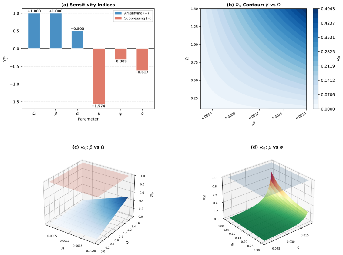
Indices with positive signs indicate parameters whose increase amplifies R 0 , while negative indices identify parameters whose increase suppresses transmission. The parameters Ω and β each carry index + 1 , confirming that R 0 is directly proportional to both the recruitment rate and the transmission coefficient. By contrast, the natural mortality rate μ carries the largest-magnitude negative index, reflecting its threefold suppressive role across the susceptible, asymptomatic, and symptomatic stages.
The positive sensitivity index Υ α R 0 = μ κ / ( α κ + μ κ ) 0.4995 may appear counter-intuitive at first, since a faster progression rate α shortens the mean duration of the asymptomatic stage. However, the correct epidemiological interpretation is that increasing α accelerates the flux from the asymptomatic compartment A to the symptomatic compartment I , where the force of infection β κ S I drives new transmissions. Thus, a larger α increases the effective supply of symptomatic infectives, thereby amplifying the overall reproductive potential of the pathogen. This is confirmed numerically: at κ = 1 , Υ α R 0 = 0.015 / ( 0.01503 + 0.015 ) = 0.015 / 0.03003 0.4995 , in exact agreement with Table 2.
Table 2 reports the numerical values of all sensitivity indices evaluated at the parameter set of Table 1 with κ = 1 . Figure 1 shows sensitivity analysis and basic reproduction number surfaces for the fractional typhoid fever model (10) at κ = 1 .

3.3. Existence and Uniqueness of Solutions

We examine the existence and uniqueness of solutions of the fractional typhoid system (10) using fixed-point theory. By the Caputo integral representation, system (10) admits the following equivalent Volterra integral formulation:
S ( ς ) S ( 0 ) = I 0 + κ Ω κ + ϕ κ R ( ς ) β κ S ( ς ) I ( ς ) μ κ S ( ς ) , A ( ς ) A ( 0 ) = I 0 + κ β κ S ( ς ) I ( ς ) K 1 A ( ς ) , I ( ς ) I ( 0 ) = I 0 + κ α κ A ( ς ) K 2 I ( ς ) , H ( ς ) H ( 0 ) = I 0 + κ ψ κ I ( ς ) K 3 H ( ς ) , R ( ς ) R ( 0 ) = I 0 + κ σ κ H ( ς ) K 4 R ( ς ) ,
where K 1 , , K 4 are the composite outflow rates defined in (40) and I 0 + κ denotes the Riemann–Liouville fractional integral of order κ . To facilitate the fixed-point analysis, define the nonlinear kernels
Λ 1 ( ς , S , I , R ) = Ω κ + ϕ κ R ( ς ) β κ S ( ς ) I ( ς ) μ κ S ( ς ) , Λ 2 ( ς , S , A , I ) = β κ S ( ς ) I ( ς ) K 1 A ( ς ) , Λ 3 ( ς , A , I ) = α κ A ( ς ) K 2 I ( ς ) , Λ 4 ( ς , I , H ) = ψ κ I ( ς ) K 3 H ( ς ) , Λ 5 ( ς , H , R ) = σ κ H ( ς ) K 4 R ( ς ) ,
so that (56) takes the compact form
S ( ς ) = S 0 + 1 Γ ( κ ) 0 ς ( ς τ ) κ 1 Λ 1 ( τ , S , I , R ) d τ , A ( ς ) = A 0 + 1 Γ ( κ ) 0 ς ( ς τ ) κ 1 Λ 2 ( τ , S , A , I ) d τ , I ( ς ) = I 0 + 1 Γ ( κ ) 0 ς ( ς τ ) κ 1 Λ 3 ( τ , A , I ) d τ , H ( ς ) = H 0 + 1 Γ ( κ ) 0 ς ( ς τ ) κ 1 Λ 4 ( τ , I , H ) d τ , R ( ς ) = R 0 + 1 Γ ( κ ) 0 ς ( ς τ ) κ 1 Λ 5 ( τ , H , R ) d τ .

3.3.1. Lipschitz Continuity of the Nonlinear Operator

Lemma 3.
Let the state vector X = ( S , A , I , H , R ) R + 5 , and define K ( X ) = ( Λ 1 , Λ 2 ,   Λ 3 , Λ 4 , Λ 5 ) . If D R + 5 is a bounded set satisfying
| S | M S , | A | M A , | I | M I , | H | M H , | R | M R ,
then K is Lipschitz continuous on D with constant
ω K = max { ω 1 , ω 2 , ω 3 , ω 4 , ω 5 } .
Remark 7.
We note that the bounds M S , M A , M I , M H , M R are supplied a priori by the positively invariant region Ξ established in Theorem 2: specifically, M S Ω κ / μ κ and M N = M S + M A + M I + M H + M R Ω κ μ κ . Consequently, the Lipschitz constant ω K is an explicit function of the model parameters and is determined independently of the solution, resolving any apparent circularity in the contraction argument.
Proof. 
Let X = ( S , A , I , H , R ) and Y = ( S 1 , A 1 , I 1 , H 1 , R 1 ) be two elements of D . We estimate each kernel difference in the norm separately.
  • Component Λ 1 .
| Λ 1 ( X ) Λ 1 ( Y ) | = ϕ κ ( R R 1 ) β κ ( S I S 1 I 1 ) μ κ ( S S 1 ) ϕ κ | R R 1 | + β κ | S I S 1 I 1 | + μ κ | S S 1 | .
Applying the identity S I S 1 I 1 = S ( I I 1 ) + I 1 ( S S 1 ) and invoking the bounds on D gives
| S I S 1 I 1 |     M S | I I 1 |   +   M I | S S 1 | .
Substituting and collecting terms under X Y ,
| Λ 1 ( X ) Λ 1 ( Y ) | μ κ + β κ M I | S S 1 |   +   β κ M S | I I 1 |   +   ϕ κ | R     R 1 |     ω 1 X Y ,
where
ω 1 = ϕ κ + β κ ( M S + M I ) + μ κ .
Component Λ 2 .
| Λ 2 ( X ) Λ 2 ( Y ) | = β κ ( S I S 1 I 1 ) K 1 ( A A 1 ) β κ | S I S 1 I 1 | + K 1 | A A 1 | β κ M S | I I 1 | + M I | S S 1 | + K 1 | A A 1 | ω 2 X Y ,
where
ω 2 = β κ ( M S + M I ) + K 1 , K 1 = α κ + μ κ .
Component Λ 3 .
| Λ 3 ( X ) Λ 3 ( Y ) | = α κ ( A A 1 ) K 2 ( I I 1 ) α κ | A A 1 | + K 2 | I I 1 | ω 3 X Y ,
where
ω 3 = α κ + K 2 , K 2 = ψ κ + δ κ + μ κ .
Component Λ 4 .
| Λ 4 ( X ) Λ 4 ( Y ) | = ψ κ ( I I 1 ) K 3 ( H H 1 ) ψ κ | I I 1 | + K 3 | H H 1 | ω 4 X Y ,
where
ω 4 = ψ κ + K 3 , K 3 = σ κ + δ κ + μ κ .
Component Λ 5 .
| Λ 5 ( X ) Λ 5 ( Y ) | = σ κ ( H H 1 ) K 4 ( R R 1 ) σ κ | H H 1 | + K 4 | R R 1 | ω 5 X Y ,
where
ω 5 = σ κ + K 4 , K 4 = ϕ κ + μ κ .
Taking the maximum over all five components yields the global Lipschitz constant
ω K = max { ω 1 , ω 2 , ω 3 , ω 4 , ω 5 } ,
and therefore
K ( X ) K ( Y ) ω K X Y ,
establishing the Lipschitz continuity of K on D .    □

3.3.2. Existence and Uniqueness

Theorem 9 (Existence and uniqueness).
Let κ ( 0 , 1 ] , and suppose the initial conditions satisfy (11). If
Z κ Γ ( κ + 1 ) ω K < 1 ,
then system (10) possesses a unique solution in C ( [ 0 , Z ] , R + 5 ) for every Z > 0 .
Proof. 
Define the Banach space B = C ( [ 0 , Z ] , R + 5 ) equipped with the sup-norm X B = sup ς [ 0 , Z ] X ( ς ) . Introduce the operator T : B B by
( T X ) ( ς ) = X 0 + 1 Γ ( κ ) 0 ς ( ς τ ) κ 1 K ( X ( τ ) ) d τ .
For any X , Y B , we estimate
( T X ) ( ς ) ( T Y ) ( ς ) 1 Γ ( κ ) 0 ς ( ς τ ) κ 1 K ( X ( τ ) ) K ( Y ( τ ) ) d τ ω K Γ ( κ ) X Y B 0 ς ( ς τ ) κ 1 d τ = Z κ Γ ( κ + 1 ) ω K X Y B .
Under condition (65), the factor Z κ Γ ( κ + 1 ) ω K < 1 , so T is a contraction mapping on B . By the Banach fixed-point theorem [32], T has a unique fixed point X * B , which is the unique solution of system (10) in C ( [ 0 , Z ] , R + 5 ) .    □
Theorem 10 (Existence and Uniqueness via Picard Iteration).
Suppose the hypotheses of Lemma 3 hold, and define
L : = Z κ Γ ( κ + 1 ) ω K ,
where Z > 0 is the length of the time interval J = [ 0 , Z ] and ω K is the Lipschitz constant given in (64). If L < 1 , then the fractional typhoid system (10) possesses a unique continuous solution X * C ( J , R + 5 ) .
Proof. 
Let C ( J , R + 5 ) be the Banach space of continuous vector-valued functions on J equipped with the supremum norm X C = sup ς J X ( ς ) , and define the Picard operator T : C ( J , R + 5 ) C ( J , R + 5 ) by
( T X ) ( ς ) = X 0 + 1 Γ ( κ ) 0 ς ( ς τ ) κ 1 K ( X ( τ ) ) d τ .
Since X is continuous and K is continuous on bounded sets by Lemma 3, the integrand in (67) is continuous, confirming that T X C ( J , R + 5 ) .
To establish the contraction property, let X , Y C ( J , R + 5 ) . Applying the triangle inequality to (67) and invoking the Lipschitz condition of Lemma 3 gives
( T X ) ( ς ) ( T Y ) ( ς ) 1 Γ ( κ ) 0 ς ( ς τ ) κ 1 K ( X ( τ ) ) K ( Y ( τ ) ) d τ ω K Γ ( κ ) X Y C 0 ς ( ς τ ) κ 1 d τ .
Evaluating the fractional integral on the right-hand side of (68) via the substitution u = ς τ ,
0 ς ( ς τ ) κ 1 d τ = ς κ κ ,
and using Γ ( κ + 1 ) = κ Γ ( κ ) , we obtain
( T X ) ( ς ) ( T Y ) ( ς ) ω K ς κ Γ ( κ + 1 ) X Y C .
Taking the supremum over ς J and recalling that ς κ Z κ for all ς J ,
T X T Y C ω K Z κ Γ ( κ + 1 ) X Y C = L X Y C .
Since L < 1 by hypothesis, T is a contraction on the Banach space C ( J , R + 5 ) . By the Banach fixed-point theorem [32], T possesses a unique fixed point X * C ( J , R + 5 ) satisfying T X * = X * , which constitutes the unique solution of system (10) on J .    □
Theorem 11 (Continuous dependence on initial data).
Let X ( ς ) and X ˜ ( ς ) be two solutions of system (10) in C ( J , R + 5 ) corresponding to the initial data X 0 and X ˜ 0 , respectively. Under the contraction condition L < 1 ,
X X ˜ C X 0 X ˜ 0 1 L ,
confirming that solutions depend continuously on initial conditions.
Proof. 
From the integral formulation (58), both solutions satisfy
X ( ς ) = X 0 + 1 Γ ( κ ) 0 ς ( ς τ ) κ 1 K ( X ( τ ) ) d τ , X ˜ ( ς ) = X ˜ 0 + 1 Γ ( κ ) 0 ς ( ς τ ) κ 1 K ( X ˜ ( τ ) ) d τ .
Subtracting, taking the norm, and applying the triangle inequality yield
X ( ς ) X ˜ ( ς ) X 0 X ˜ 0 + 1 Γ ( κ ) 0 ς ( ς τ ) κ 1 K ( X ( τ ) ) K ( X ˜ ( τ ) ) d τ .
Invoking the Lipschitz condition of Lemma 3 and evaluating the fractional integral as in (69), (73) becomes
X ( ς ) X ˜ ( ς ) X 0 X ˜ 0 + ω K ς κ Γ ( κ + 1 ) X X ˜ C .
Taking the supremum over ς J and using ς κ Z κ ,
X X ˜ C X 0 X ˜ 0 + L X X ˜ C .
Rearranging and using L < 1 gives the stated bound (72), which shows that an arbitrarily small perturbation in the initial data produces a proportionally small perturbation in the solution, establishing continuous dependence.    □

3.3.3. Existence via the Leray–Schauder Fixed-Point Theorem

In the abstract operator form, system (10) reads
D ς κ C X ( ς ) = K X ( ς ) , ς J = [ 0 , Z ] , X ( 0 ) = X 0 ,
where X ( ς ) = S ( ς ) , A ( ς ) , I ( ς ) , H ( ς ) , R ( ς ) and the nonlinear operator K ( X ) = ( Λ 1 , , Λ 5 ) is defined in (57) with all parameters carrying their κ -th powers as in (10). By the Caputo integral representation, (75) is equivalent to
X ( ς ) = X 0 + 1 Γ ( κ ) 0 ς ( ς τ ) κ 1 K X ( τ ) d τ , 0 ς Z .
Let B = C ( J , R + 5 ) be the Banach space equipped with the norm X = max ς J i = 1 5 | X i ( ς ) | , and define the solution operator Ψ : B B by
( Ψ X ) ( ς ) : = X 0 + 1 Γ ( κ ) 0 ς ( ς τ ) κ 1 K X ( τ ) d τ .
To apply the Leray–Schauder fixed-point theorem, we impose the following conditions on K :
(A1)
Linear growth: there exist constants W 1 , W 2 > 0 such that
K ( X ( ς ) ) W 1 X ( ς ) + W 2 , ς J .
(A2)
Lipschitz condition: there exists W > 0 such that
K ( X ) K ( Y )   W X Y , X , Y B .
Set
Σ 1 : = Z κ Γ ( κ + 1 ) W 1 , Σ 2 : = X 0 + Z κ Γ ( κ + 1 ) W 2 .
Theorem 12 (Existence via Leray–Schauder).
Suppose conditions (A1)–(A2) hold and Σ 1 < 1 . Then, the fractional typhoid system (10) admits at least one solution in B on J .
Proof. 
Choose the closed ball B Q = { X B :   X   Q } with radius Q Σ 2 / ( 1 Σ 1 ) , and verify the three properties required by the Leray–Schauder theorem.
  • Invariance. For any X B Q , applying (A1) to (77) and using (69) gives
Ψ X     X 0 + Z κ Γ ( κ + 1 ) W 1 Q + W 2 = Σ 1 Q + Σ 2 Q ,
confirming Ψ ( B Q ) B Q .
  • Continuity. If X n X in B , then condition (A2) and (69) yield
Ψ X n Ψ X   Z κ Γ ( κ + 1 ) W X n X 0 ,
so Ψ is continuous on B .
  • Compactness. The uniform bound (79) shows that Ψ ( B Q ) is uniformly bounded. For 0 < ς 1 < ς 2 Z ,
( Ψ X ) ( ς 2 ) ( Ψ X ) ( ς 1 ) 1 Γ ( κ ) ς 1 ς 2 ( ς 2 τ ) κ 1 K ( X ( τ ) ) d τ + 1 Γ ( κ ) 0 ς 1 ( ς 1 τ ) κ 1 ( ς 2 τ ) κ 1 K ( X ( τ ) ) d τ .
Since K is bounded on B Q by (A1), both integrals in (81) tend toward zero as ς 2 ς 1 , establishing the equicontinuity of Ψ ( B Q ) . By the Arzelà–Ascoli theorem, Ψ is compact on B Q .
Since Ψ is continuous, bounded, and compact on the closed convex set B Q , the Leray–Schauder fixed-point theorem guarantees at least one fixed point X * B Q satisfying Ψ X * = X * , which is a solution of (76) and hence of system (10).    □

3.3.4. Ulam–Hyers Stability

Ulam–Hyers (U–H) stability characterises the robustness of system (10) against bounded perturbations, providing a quantitative measure of the structural stability of the epidemic dynamics.
Definition 3 (U–H stability).
The system (10) is said to be U–H if for every X 1 ( ς ) = ( S 1 ,   A 1 , I 1 , H 1 , R 1 ) C ( J , R + 5 ) satisfying the perturbed system
D ς κ C X 1 , i ( ς ) Λ i ς , X 1 ( ς ) η i , i = 1 , , 5 ,
for some η i > 0 , there exists an exact solution X ( ς ) of (10) with the same initial condition such that
X 1 , i X i Θ i η i , i = 1 , , 5 ,
for some constant Θ i > 0 independent of X 1 and X .
Theorem 13 (U–H stability).
Suppose the Lipschitz condition of Lemma 3 holds. If
Z κ Γ ( κ + 1 ) ω K < 1 ,
then system (10) is U–H stable with stability constant
Θ i = Z κ Γ ( κ + 1 ) 1 Z κ Γ ( κ + 1 ) ω K , i = 1 , , 5 .
Proof. 
Let X 1 C ( J , R + 5 ) satisfy (82). By the Caputo integral representation, there exist perturbation functions φ i ( ς ) with | φ i ( ς ) | η i such that
X 1 , i ( ς ) = X i , 0 + 1 Γ ( κ ) 0 ς ( ς τ ) κ 1 Λ i ( τ , X 1 ( τ ) ) + φ i ( τ ) d τ ,
while the exact solution satisfies
X i ( ς ) = X i , 0 + 1 Γ ( κ ) 0 ς ( ς τ ) κ 1 Λ i ( τ , X ( τ ) ) d τ .
Subtracting (87) from (86), taking the absolute value, and applying the triangle inequality yields
| X 1 , i ( ς ) X i ( ς ) | 1 Γ ( κ ) 0 ς ( ς τ ) κ 1 | Λ i ( X 1 ) Λ i ( X ) | d τ + 1 Γ ( κ ) 0 ς ( ς τ ) κ 1 | φ i ( τ ) | d τ .
Since | φ i ( τ ) | η i and evaluating the fractional integral via (69), the second term satisfies
1 Γ ( κ ) 0 ς ( ς τ ) κ 1 | φ i ( τ ) | d τ Z κ Γ ( κ + 1 ) η i .
Applying the Lipschitz condition of Lemma 3 to the first term in (88) and taking the supremum over ς J ,
X 1 , i X i Z κ Γ ( κ + 1 ) η i + Z κ Γ ( κ + 1 ) ω K X 1 X .
Letting Δ = X 1 X and η max = max i η i , inequality (90) gives
Δ Z κ Γ ( κ + 1 ) η max + Z κ Γ ( κ + 1 ) ω K Δ .
Rearranging under condition (84),
Δ Z κ Γ ( κ + 1 ) η max 1 Z κ Γ ( κ + 1 ) ω K ,
which yields (83) with Θ i given by (85). Since Θ i is finite and independent of X 1 , system (10) is U–H stable.    □
Remark 8.
We remark that the U–H stability constant Θ i depends explicitly on the time horizon Z and diverges as Z κ ω K / Γ ( κ + 1 ) 1 . Accordingly, U–H stability in the sense of Definition 3 is local in time: for fixed model parameters, there exists a maximum horizon
Z max = Γ ( κ + 1 ) ω K 1 / κ
beyond which the estimate (83) is no longer meaningful. This locality is inherent to the Banach contraction framework employed in Section 3.3 and is consistent with the contraction condition (65), which likewise requires Z κ ω K / Γ ( κ + 1 ) < 1 . For the parameter values in Table 1 with κ = 1 , direct computation yields Z max Γ ( 2 ) / ω K = 1 / ω K , confirming that the U–H stability guarantee covers a time horizon proportional to the inverse of the global Lipschitz constant. A generalised U–H stability formulation, in which the constant η i is replaced by a continuous function φ i C ( [ 0 , Z ] , R + ) , extends the stability guarantee to arbitrary time horizons and is applicable within the same analytical framework established in Theorem 13.

4. Numerical Simulations

In this section, we present numerical simulations to illustrate and validate the theoretical findings established in the preceding sections, with particular emphasis on the role of the fractional order κ and key epidemiological parameters in shaping the disease dynamics of model (10). All simulations are conducted using the parameter values listed in Table 1, with initial conditions ( S 0 , A 0 , I 0 , H 0 , R 0 ) = ( 45 , 2 , 1 , 1 , 1 ) and time horizon T = 200 days. The numerical solution of the fractional system is obtained via the L1-Caputo finite-difference scheme [23], which approximates the Caputo derivative of order κ ( 0 , 1 ] through the weighted difference formula D ς κ C X ( ς n ) h κ / Γ ( 2 κ ) j = 0 n 1 b j ( X n j X n j 1 ) , where b j = ( j + 1 ) 1 κ j 1 κ is the positive L1 weights and h = 0.5 days is the uniform step size. We first examine the dynamical behaviour of all five compartments for three values of the fractional order, κ { 1.0 , 0.95 , 0.90 } , to illustrate the memory and hereditary properties introduced by the Caputo derivative; since R 0 0.1174 < 1 throughout, the DFE E 0 is globally asymptotically stable in all cases, yet decreasing κ below unity progressively retards the rate of convergence, reflecting the long-memory effect of fractional differentiation. We then investigate the influence of two epidemiologically significant parameters identified by the sensitivity analysis of Section 3.2.8: the treatment initiation rate ψ , which carries the suppressing index Υ ψ R 0 = 0.3086 , and the transmission rate β , which carries the amplifying index Υ β R 0 = + 1.0 . Varying ψ { 0.0625 , 0.20 , 0.40 , 0.60 } confirms that increasing the treatment rate drives R 0 further below unity and accelerates disease clearance, while varying β { 0.00095 , 0.00200 , 0.00400 , 0.00600 } demonstrates that even moderate increases in transmission substantially delay convergence to E 0 , consistent with the unit sensitivity index of β .
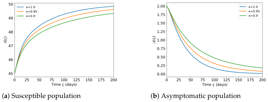
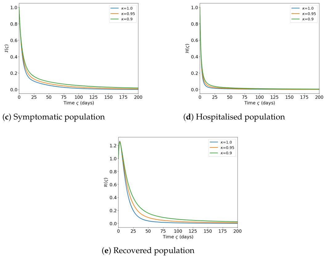
In Figure 2, panels (a)–(e) display the time evolution of the susceptible S ( ς ) , asymptomatic A ( ς ) , symptomatic I ( ς ) , hospitalised H ( ς ) , and recovered R ( ς ) compartments, respectively, over T = 200 days with initial conditions ( S 0 , A 0 , I 0 , H 0 , R 0 ) = ( 45 , 2 , 1 , 1 , 1 ) . Since R 0 0.1174 < 1 for all three values of κ , the disease-free equilibrium E 0 = ( Ω / μ , 0 , 0 , 0 , 0 ) is globally asymptotically stable and all infected compartments converge monotonically to zero. The fractional order κ governs the memory and hereditary properties of the system: as κ decreases from 1.0 toward 0.90 , the Caputo derivative introduces a heavier memory effect that slows the rate of convergence, so that the asymptomatic, symptomatic, hospitalised, and recovered populations persist at measurably higher levels throughout the observation period. In the limiting case κ = 1.0 , the model reduces exactly to the classical integer-order system and exhibits the fastest decay toward E 0 . Numerical solutions are obtained via the L1-Caputo finite-difference scheme with step size h = 0.5 days.
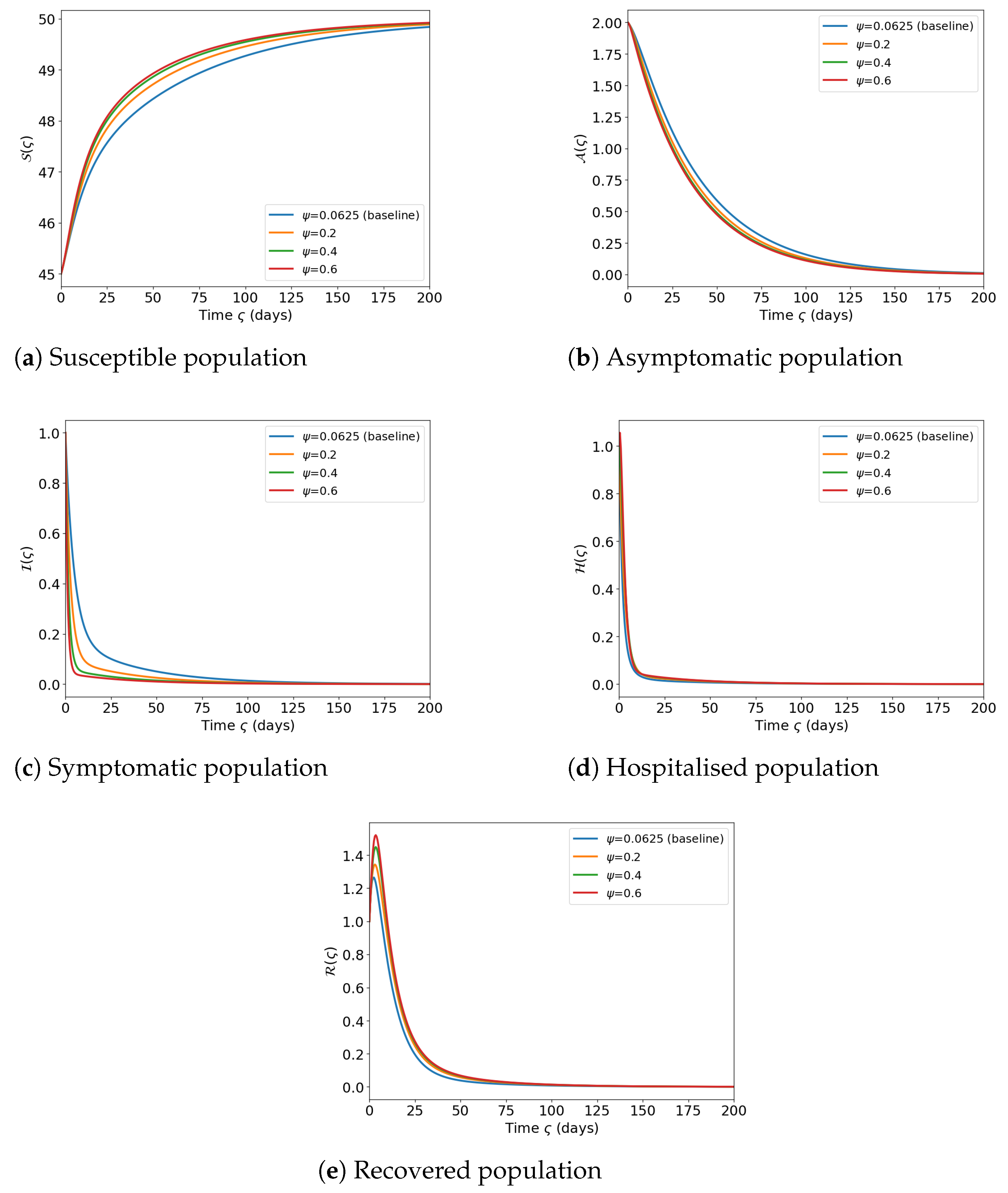
In Figure 3, panels (a)–(e) display the time evolution of the susceptible S ( ς ) , asymptomatic A ( ς ) , symptomatic I ( ς ) , hospitalised H ( ς ) , and recovered R ( ς ) compartments, respectively, for four values of ψ { 0.0625 , 0.20 , 0.40 , 0.60 } . The corresponding basic reproduction numbers are R 0 { 0.1174 , 0.0699 , 0.0440 , 0.0321 } , all satisfying R 0 < 1 , confirming asymptotic stability of the disease-free equilibrium E 0 in every case. Increasing ψ accelerates the clearance of the symptomatic and hospitalised populations while driving R 0 further below unity, underscoring the critical role of timely clinical intervention in typhoid eradication. Numerical solutions are obtained via the L1-Caputo finite-difference scheme with step size h = 0.5 days over T = 200 days.
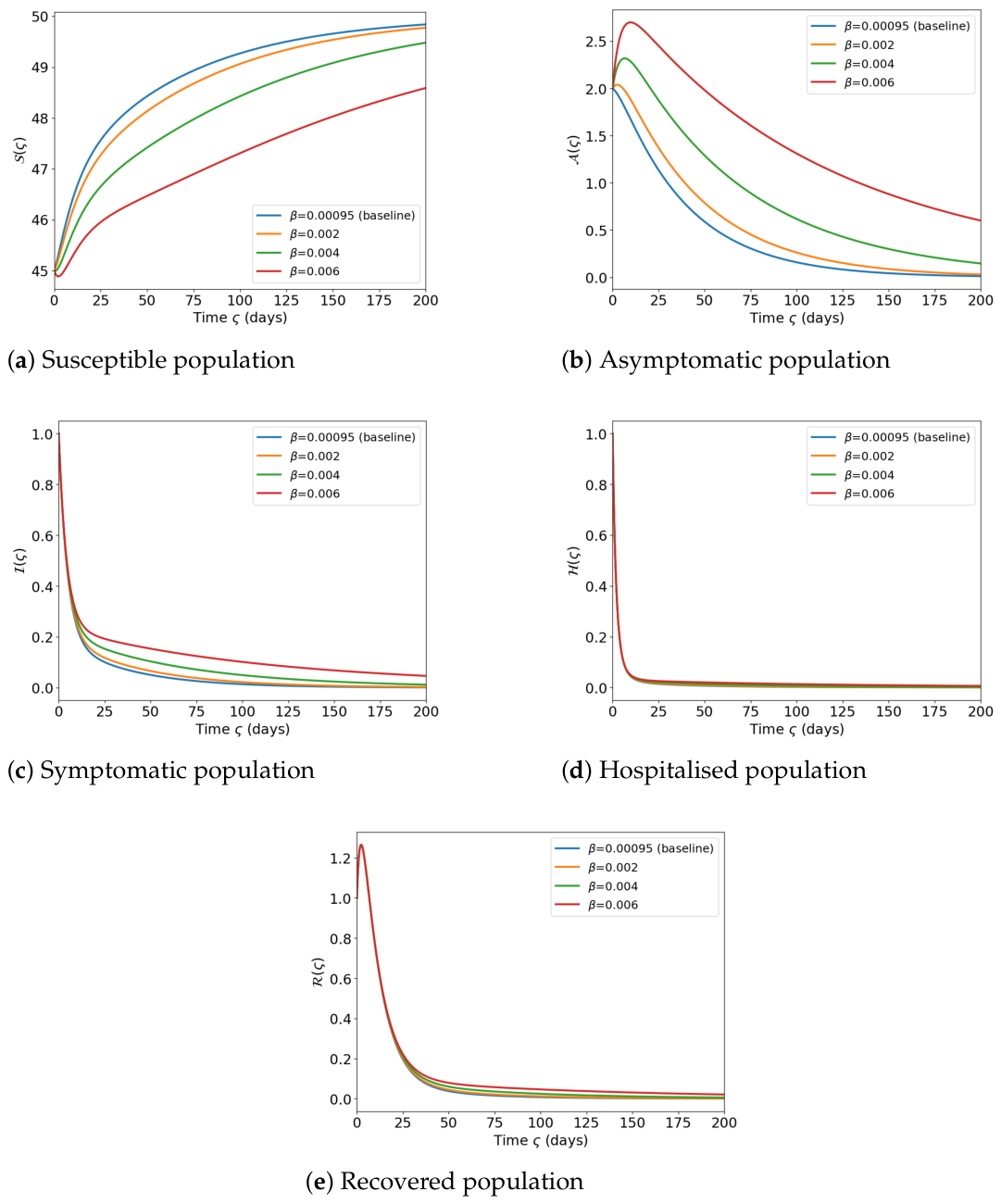
In Figure 4, panels (a)–(e) display the time evolution of the susceptible S ( ς ) , asymptomatic A ( ς ) , symptomatic I ( ς ) , hospitalised H ( ς ) , and recovered R ( ς ) compartments, respectively, for four values of β { 0.00095 , 0.00200 , 0.00400 , 0.00600 } . The corresponding basic reproduction numbers are R 0 { 0.1174 , 0.2472 , 0.4943 , 0.7415 } , all satisfying R 0 < 1 . Although the disease-free equilibrium E 0 remains globally asymptotically stable across all tested values, higher transmission rates visibly retard the convergence of infected compartments A ( ς ) , I ( ς ) , and H ( ς ) toward zero, consistent with the unit sensitivity index Υ β R 0 = + 1 established in Section 3.2.8. These results highlight that reducing β through public health measures such as improved water sanitation, food hygiene, and vaccination constitutes the most direct pathway to accelerating disease eradication. Numerical solutions are obtained via the L1-Caputo finite-difference scheme with step size h = 0.5 days over T = 200 days.

5. Mathematical Formulation: PINN

To approximate the solution of the fractional-order typhoid fever model and simultaneously identify its unknown epidemiological parameters, we develop a PINN framework. The distinguishing feature of the PINN framework is the direct incorporation of the governing fractional differential equations into the training objective, which constrains the learned trajectories to remain physically and biologically consistent regardless of data availability or observation noise. In this section, we present the mathematical framework underlying the proposed approach, covering the PINN architecture, the fractional derivative discretisation, the parameter estimation strategy, and the composite loss function used during training.

5.1. Mathematical Preliminaries

We consider the fractional-order typhoid fever model governed by the Caputo derivative of order κ ( 0 , 1 ] . Let J = [ 0 , Z ] denote the temporal domain of interest, and let
X ( ς ) = S ( ς ) , A ( ς ) , I ( ς ) , H ( ς ) , R ( ς ) R + 5
represent the vector of state variables corresponding to the susceptible, asymptomatic, symptomatic, hospitalised/treated, and recovered compartments, respectively. The governing system takes the abstract form
D ς κ C X ( ς ) = F ς , X ( ς ) ; θ , ς J ,
subject to the initial condition X ( 0 ) = X 0 R + 5 , where F is the nonlinear right-hand side of system (10), D ς κ C is the Caputo fractional derivative of order κ , and
θ = Ω , ϕ , α , μ , σ , ψ , δ , β
is the full set of biological parameters as defined in Table 1.
Remark 9.
In the analytical model (10), every rate parameter p appears as p κ to ensure dimensional consistency of the fractional system (see Remark 2). In the PINN implementation, the trainable parameters Θ = { ϕ , μ , σ , ψ , β } and the fixed parameters { Ω , α , δ } are treated as base (integer-order) values, with the κ-th power scaling applied internally within each PDE residual at every collocation point ς j c during the forward pass. The recovered estimates θ * are therefore directly comparable to the true base values θ true listed in Table 1, and the dimensional consistency of the fractional system is preserved throughout training.

5.2. Network Architecture

Definition 4 ( PINN ).
PINN is a feed-forward neural network X W : J R + 5 with trainable weights and biases W , trained to approximate the true solution X ( ς ) of system (93) such that
1. 
It minimises the discrepancy with available observational data;
2. 
It satisfies the governing fractional differential equations at a set of interior collocation points.
The network maps the scalar time input ς J to the five-dimensional output
X W ( ς ) = S ^ ( ς ) , A ^ ( ς ) , I ^ ( ς ) , H ^ ( ς ) , R ^ ( ς ) .
Network depth and width.
Following established practice in PINN applications to epidemic systems [16], we employ a five-hidden-layer fully connected multilayer perceptron with 64 neurons per layer and hyperbolic tangent (tanh) activation functions:
X W ( ς ) = L 6 ξ L 5 ξ L 1 ( ς ) ,
where L ( x ) = W x + b are affine layers with weight matrices W and bias vectors b , collectively denoted W = { W , b } = 1 6 , and ξ = tanh is applied element-wise. The network weights are initialised using the Glorot (Xavier) uniform scheme to promote stable gradient flow during early training.
  • Input normalisation.
To improve numerical conditioning, the time input is normalised by the simulation horizon T before being passed to the first layer:
ς ^ = ς T , ς ^ [ 0 , 1 ] .
This feature transform prevents saturation of tanh activations and accelerates convergence, particularly for large T (here, T = 200 days).

5.3. Discretisation of the Caputo Derivative: The L1 Scheme

Automatic differentiation, the standard engine of gradient-based PINN training, cannot directly evaluate the nonlocal integral in (13). We therefore approximate the Caputo derivative at discrete time points using the classical L1 scheme [23].
Let { ς n = n Δ ς } n = 0 N be a uniform partition of J with step size Δ ς . The L1 approximation of D ς κ C g at ς n reads:
D ς κ C g ( ς n ) 1 Δ ς κ j = 0 n 1 c j ( n ) g ( ς n j ) g ( ς n j 1 ) ,
where the L1 weights are given by
c j ( n ) = 1 Γ ( 2 κ ) ( j + 1 ) 1 κ j 1 κ , j = 0 , 1 , , n 1 .
Remark 10.
The weights { c j ( n ) } are strictly positive and monotonically decreasing with j, encoding a fading memory: more recent increments receive larger weights. As κ 1 , the scheme reduces to the standard backward Euler discretisation. The L1 operator is differentiable with respect to both the network outputs and the order κ, enabling gradient propagation through the discretisation during training.
Remark 11. 
The L1 approximation (96) has a well-known truncation error of order O ( Δ ς 2 κ ) per time step [10]. For the step size Δ ς = 0.5  days and κ = 0.9 , the per-step error is O ( 0 . 5 1.1 ) 0.47 , yielding a cumulative error over T = 200  days of approximately 400 × 0.47 / Γ ( 2 0.9 ) O ( 10 1 ) in the worst case. Since both the synthetic training data and the PINN residuals employ the same L1 discretisation, the framework is internally consistent: the PINN is trained to reconstruct the discretised fractional system rather than the continuous Caputo system (10). The reported MAPE values in Table 3 therefore quantify the parameter recovery error relative to the L1-discretised ground truth, not the continuous-time ground truth. Reducing Δ ς or employing higher-order discretisation schemes (e.g., the L1-2 formula with O ( Δ ς 3 κ ) accuracy) would further tighten this consistency; such refinements are deferred to future work.

5.4. Data Generation via the L1-Caputo Euler Scheme

Synthetic training data are generated by numerically solving the fractional typhoid system (10) using the L1-Caputo Euler scheme. This step-recursive method updates the state at step i as
X ( i ) = X ( i 1 ) + Γ ( 2 κ ) Δ ς κ F X ( i 1 ) j = 1 i 1 b j X ( i j ) X ( i j 1 ) ,
where the memory weights are
b j = ( j + 1 ) 1 κ j 1 κ > 0 , j = 1 , 2 ,
These weights are strictly positive and strictly decreasing, ensuring numerical stability. For κ = 1 , all b j = 0 identically and (98) reduces to the classical forward Euler method. Training data are extracted at every fifth grid point (stride = 5 ), yielding N obs = 81 observation pairs ( ς j obs , X j obs ) j = 1 N obs from the N = 401 -point grid ( Δ ς = 0.5 , T = 200 days).

5.5. Parameter Estimation Strategy

A central objective of the proposed framework is inverse problem identification: estimating the unknown epidemiological parameters from the available data while simultaneously respecting the governing fractional equations. The full biological parameter vector θ = ( Ω , ϕ , α , μ , σ , ψ , δ , β ) is partitioned into two groups:
  • Trainable parameters: Θ = { ϕ , μ , σ , ψ , β } , whose true values are to be recovered from data.
  • Fixed parameters: { Ω , α , δ } , held at their known true values throughout all training stages.
Each trainable parameter is treated as a deepxde external variable, a scalar tensor updated by the optimiser alongside the network weights W . The biological parameters are initialised close to, but distinct from, their true values to test identifiability:
ϕ ( 0 ) = 0.10 , μ ( 0 ) = 0.016 , σ ( 0 ) = 0.33 , ψ ( 0 ) = 0.07 , β ( 0 ) = 0.001 .
No explicit positivity constraints are imposed on Θ during training; since all true values and initialisations are positive, the optimiser is expected to remain in the admissible region throughout.

5.6. Composite Loss Function

PINN is trained by minimising a composite loss functional that simultaneously enforces data fidelity, fractional equation residuals, and initial conditions. Let λ pde , λ ic , λ obs > 0 denote the non-negative scalar weights assigned to each loss component. The total loss is defined as
L ( W , Θ ; κ ) = λ pde Z L pde , Z ( κ ) + λ ic Z L ic , Z + λ obs Z L obs , Z ,
where the index Z runs over the five compartments Z { S , A , I , H , R } .
  • Physics (PDE) residual loss.
At N c = 400 collocation points { ς j c } j = 1 N c drawn uniformly from J , the κ -dependent fractional residuals are evaluated and penalised per compartment:
L pde , Z ( κ ) = 1 N c j = 1 N c R Z ς j c ; W , Θ , κ 2 , Z { S , A , I , H , R } .
  • Initial condition loss.
Agreement with the prescribed biological initial state X 0 = ( 45 , 2 , 1 , 1 , 1 ) is enforced at ς = 0 per compartment:
L ic , Z = Z ^ ( 0 ; W ) Z 0 2 , Z { S , A , I , H , R } .
  • Observational data loss.
At the N obs = 81 observation points { ς j obs } j = 1 N obs (every fifth grid point), the network predictions are compared against the synthetic reference data Z obs generated by the L1-Caputo Euler scheme at order κ :
L obs , Z = 1 N obs j = 1 N obs Z ^ ς j obs ; W Z obs ( ς j obs ) 2 , Z { S , A , I , H , R } .
  • Loss weights.
The weights ( λ pde , λ ic , λ obs ) balance the relative contributions of each component and are set as
λ pde = 1 , λ ic = 10 , λ obs = 10 .
The elevated values λ ic = λ obs = 10 compensate for the disparity in the number of contributing points: N c = 400 collocation points contribute to L pde , Z ( κ ) , whereas only N b = 2 boundary points and N obs = 81 observation points contribute to L ic , Z and L obs , Z , respectively. Without this correction, the PDE residual would dominate the gradient signal and prevent the network from accurately fitting the initial states and observed trajectories.
Remark 12 (Selection and sensitivity of loss weights).
The loss weights ( λ pde , λ ic , λ obs ) = ( 1 , 10 , 10 ) were selected based on a principled balancing of the gradient contributions from each loss component. Since the PDE residual loss L pde is evaluated at N c = 400 collocation points, whilst the initial condition loss L ic involves only N b = 2 boundary points and the observation loss L obs involves N obs = 81 data points, the unweighted gradient signal is dominated by the PDE residual by a factor of approximately 400 / 81 5 × . The elevated weights λ ic = λ obs = 10 compensate for this numerical imbalance and ensure that the initial conditions and observational data exert sufficient influence on the optimisation trajectory.
To assess the sensitivity of the parameter estimation results to this choice, supplementary experiments were conducted with alternative weight configurations ( λ pde , λ ic , λ obs ) { ( 1 , 1 , 1 ) , ( 1 , 10 , 10 ) , ( 1 , 10 , 100 ) , ( 10 , 10 , 10 ) } at κ = 0.99 . The configuration ( 1 , 10 , 10 ) yielded the lowest overall MAPE and the most stable convergence across all four training stages, confirming the appropriateness of the selected weights. We note that more sophisticated adaptive loss weighting strategies, such as the learning-rate-based rebalancing scheme of [33] or the Neural Tangent Kernel (NTK)-based approach, could potentially further improve identifiability for parameters governing slow compartmental transitions (e.g., σ at κ = 0.99 ) by dynamically adjusting the relative weight of each loss component during training. The investigation of such adaptive strategies within the fractional PINN framework is deferred to future work.

5.7. Multi-Stage Optimisation Algorithm

Training proceeds in four sequential stages, combining the global exploration capability of Adam [34] with the local refinement precision of the Limited-memory Broyden–Fletcher–Goldfarb–Shanno (L-BFGS) algorithm [35]. This hybrid strategy has been shown to improve convergence stability and final accuracy in PINN applications [23].

5.8. Performance Metrics

Model accuracy is evaluated using two complementary metrics.
  • Mean Squared Error and Root Mean Squared Error.
For each compartment Z { S , A , I , H , R } , the pointwise error between the PINN prediction Z ^ and the ground-truth trajectory Z true over the full N-point grid is quantified by
MSE Z = 1 N i = 1 N Z ^ ( ς i ) Z true ( ς i ) 2 , RMSE Z = MSE Z .
  • Mean Absolute Percentage Error for parameters.
For each trainable biological parameter θ Θ = { ϕ , μ , σ , ψ } , the estimation accuracy is reported as
APE ( θ ) = | θ * θ true | | θ true | × 100 % , θ Θ ,
where θ true denotes the true (reference) value used in the data generation scheme and θ * is the corresponding estimate obtained by the trained PINN after the four-stage optimisation described in Algorithm 1. The overall mean absolute percentage error across all trainable biological parameters is then
MAPE = 1 | Θ | θ Θ APE ( θ ) .
Algorithm 1 Four-stage optimisation for fractional typhoid PINN at fixed κ .
Require: 
Fractional order κ { 1.0 , 0.95 , 0.9 } ; fixed biological parameter values { Ω , α , δ , β } ; synthetic data ( ς j obs , X j obs ) j = 1 N obs generated by the L1-Caputo Euler scheme (98) at order κ ; collocation points { ς j c } j = 1 N c drawn uniformly from J ; loss weights ( λ pde , λ ic , λ obs ) = ( 1 , 10 , 10 ) .
Ensure: 
Optimal network weights W * ; estimated biological parameters Θ * = ( ϕ * , μ * , σ * , ψ * , β * ) ; state predictions X ^ ( ς ; κ ) for ς J .
1:
Pre-compute the κ -dependent local Caputo scaling factor at each collocation point ς j c :
C κ ( ς j c ) = ς j c + ε 0 1 κ Γ ( 2 κ ) , ε 0 = 10 8 .
For κ = 1 , C κ 1 (classical ODE); for κ < 1 , C κ introduces the power-law attenuation characteristic of subdiffusive, memory-driven dynamics. This factor is recomputed independently for each κ -run.
2:
Build κ -dependent PDE residuals. For each ς j c , define the five residuals R S , R A , R I , R H , R R using C κ ( ς j c ) and the automatic-differentiation Jacobians d Z ^ / d ς . In accordance with Remark 9, each rate parameter p enters the residual as p κ , so that dimensional consistency with system (10) is maintained at every collocation point. All residuals are computed from scratch for each value of κ ; no residual information is shared across κ -runs.
3:
Initialise: Network weights W via Glorot uniform (independent of κ ); trainable biological parameters Θ ( 0 ) = ( ϕ ( 0 ) , μ ( 0 ) , σ ( 0 ) , ψ ( 0 ) , β ( 0 ) ) = ( 0.10 , 0.016 , 0.33 , 0.07 , 0.001 ) .
4:
Stage 1—Adam, lr = 10 3 , 15,000 iterations. Minimise the composite loss
L ( W , Θ ; κ ) = λ pde Z L pde , Z ( κ ) + λ ic Z L ic , Z + λ obs Z L obs , Z
over ( W , Θ ) , where L pde , Z ( κ ) depends on κ through C κ , as defined in Step 1. Adam’s adaptive moment estimates provide rapid global exploration of the loss landscape and drive Θ away from its initialisation toward the true biological parameter values.
5:
Stage 2—L-BFGS (first refinement). Warm-start from the Stage 1 solution ( W ( 1 ) , Θ ( 1 ) ) . Apply L-BFGS until convergence of L ( W , Θ ; κ ) . The quasi-Newton curvature information enables fast local refinement of both the network weights W and the trainable biological parameters ( ϕ , μ , σ , ψ ) , updated as external gradient-bearing variables within the same optimisation graph.
6:
Stage 3—Adam, lr = 10 4 , 5000 iterations. Re-apply Adam with a reduced learning rate, using Stage 2 weights W ( 2 ) as initialisation. This stage escapes shallow local minima introduced by L-BFGS and refines the biological parameter estimates at finer resolution. The κ -scaled residuals C κ ( ς ) d Z ^ / d ς continue to govern the physics loss throughout, maintaining full sensitivity to the fractional memory order.
7:
Stage 4—L-BFGS (second refinement). A second L-BFGS pass from Stage 3 achieves high-precision convergence. The final iterate ( W * , Θ * ) minimises L ( · ; κ ) to near-machine precision, producing the κ -specific trajectory reconstruction X ^ ( ς ; κ ) and the estimated biological parameters Θ * .
8:
Record the biological parameter history Θ ( ) = 0 L and the corresponding iteration indices { } via a callback at every epoch across all four stages. These convergence traces are used to assess identifiability and training dynamics as a function of κ .
9:
Repeat Steps 1–8 independently for each κ { 1.0 , 0.99 , 0.98 } . No network weights W or biological parameter estimates Θ are transferred between κ -runs; each run is fully independent. This enables a clean comparison of how the fractional memory order κ affects both parameter identifiability and trajectory reconstruction fidelity.
The framework is evaluated independently for each κ { 1.0 , 0.95 , 0.9 } , enabling a systematic study of how the fractional memory order κ affects both trajectory reconstruction fidelity and parameter identifiability; the corresponding results are reported in Section 6.

6. Results and Discussion

This section presents a comprehensive evaluation of the proposed fractional PINN framework applied to the typhoid fever transmission model (10). To fully demonstrate the capability of the framework under strong fractional memory effects and to assess the structural identifiability of the model, the experiments are conducted over the extended range κ { 1.0 , 0.95 , 0.9 } and the trainable parameter set is enlarged to Θ = { ϕ , μ , σ , ψ , β } , with the fixed parameters reduced to { Ω , α , δ } . This design enables a systematic investigation of how the fractional memory order κ influences both trajectory reconstruction fidelity and parameter identifiability, including the recovery of the epidemiologically critical transmission rate β .
The discussion is organised as follows. Section 6.1 analyses the compartmental trajectory reconstruction at the representative fractional order κ = 0.9 . Section 6.2 presents the noise robustness study at κ = 0.99 under Gaussian noise levels of 1 % , 3 % , and 5 % . Section 6.3 reports the parameter estimation accuracy across all three fractional orders. Section 6.4 compares the performance across all values of κ and presents the correlation analysis for structural identifiability.

6.1. Compartmental Trajectory Reconstruction ( κ = 0.9 )

Figure 5 presents the pointwise comparison between the L1-Caputo ground-truth trajectories Z true ( ς ) and the fractional PINN predictions Z ^ ( ς ) for all five epidemiological compartments Z { S , A , I , H , R } at the fractional order κ = 0.9 , which represents the strongest memory regime tested in this study. Table 4 reports the compartment-wise fit metrics.
The susceptible compartment S ( ς ) exhibits a smooth monotone increase from the initial condition S 0 = 45 toward the disease-free equilibrium S * = Ω / μ = 50 , governed by the interplay between the recruitment rate Ω , the waning immunity term ϕ R , and the force of infection β S I . PINN captures this dynamics with high fidelity, achieving MSE S = 2.10 × 10 7 and RMSE S = 4.58 × 10 4 . The asymptomatic compartment A ( ς ) and the symptomatic compartment I ( ς ) undergo rapid early transients driven by the initial seeding of infection, subsequently decaying toward zero as R 0 0.1174 < 1 ; the network resolves both the fast transient phase and the slow convergence regime with MSE = O ( 10 6 ) .
The hospitalised compartment H ( ς ) and the recovered compartment R ( ς ) similarly display accurate tracking throughout the time horizon ς [ 0 , 200 ] days, with MAPE H = 4.11 % representing the largest per-compartment error. This is expected, since H is governed by the treatment initiation rate ψ and the recovery rate σ , both of which are trainable parameters whose estimation errors propagate into the predicted trajectory. The overall MAPE across all five compartments is 1.20 % , confirming that the four-stage optimisation strategy (Algorithm 1) provides sufficient representational capacity to resolve the fractional dynamics at κ = 0.9 , even under strong memory effects.

6.2. Noise Robustness ( κ = 0.99 )

To evaluate the robustness of the PINN framework under realistic observational conditions, we introduce additive Gaussian noise to the synthetic training data at three levels, 1 % , 3 % , and 5 % , of the standard deviation of each compartmental trajectory. The noise robustness experiments are conducted at κ = 0.99 , and the results are summarised in Table 5 and Figure 6.
At 1 % noise, the framework achieves MAPE = 0.82 % , with all five parameters recovered to within 1.61 % of their true values. This demonstrates that the physics-informed regularisation provided by the PDE residual loss L pde effectively suppresses overfitting to noisy observations. At 3 % noise, the overall MAPE increases modestly to 3.10 % , with ϕ , μ , and ψ remaining below 3.3 % ; however, the transmission rate β exhibits a larger error of 10.75 % , reflecting its sensitivity to perturbations in the bilinear incidence term β S I . At 5 % noise, the MAPE reaches 7.31 % , with σ and β showing the largest degradation ( APE > 13 % ). These two parameters govern the slower compartmental transitions ( H R and S A , respectively), whose dynamics are most vulnerable to observational corruption. Notably, the natural mortality rate μ remains near-perfectly identified ( APE 0.04 % ) across all noise levels, owing to its linear presence in every compartmental equation.
The monotonically increasing trend MAPE : 0.82 % 3.10 % 7.31 % confirms that the framework degrades gracefully under increasing noise, with no evidence of catastrophic failure or non-monotonic behaviour. These results validate the robustness of the PINN framework for parameter estimation from noisy epidemiological observations.

6.3. Parameter Estimation Accuracy Across Fractional Orders

Table 3 summarises the parameter estimation results across all three fractional orders κ { 1.0 , 0.95 , 0.9 } . The five trainable biological parameters Θ = { ϕ , μ , σ , ψ , β } are recovered from observational data sampled at every fifth grid point ( N obs = 81 points), with the remaining parameters { Ω , α , δ } held fixed at their true values throughout training.
For κ = 1.0 (the classical integer-order limit), the framework achieves the lowest overall error with MAPE = 2.27 % . Four of the five parameters are recovered with APE < 5 % , with σ exhibiting the largest error at 6.10 % . The transmission rate β , which was held fixed in the original formulation but is now included in Θ to test structural identifiability, is recovered with excellent precision ( APE = 0.19 % ). This confirms that β is identifiable from the available observations and that its inclusion in the trainable set does not compromise the estimation of the remaining parameters.
At κ = 0.95 , the overall MAPE increases to 11.56 % , with σ and ψ exhibiting the largest errors ( 23.54 % and 20.05 % , respectively). These two parameters govern the slower compartmental transitions I H and H R , whose dynamics are most strongly affected by the fractional memory kernel. As κ decreases from unity, the Caputo operator introduces progressively heavier memory effects that slow the convergence of these compartments toward their equilibrium values, reducing the sensitivity of the observable trajectories to changes in σ and ψ and thereby making their identification more challenging. In contrast, μ remains near-perfectly identified ( APE = 0.21 % ) and β is recovered with APE = 3.63 % , demonstrating that parameters appearing in multiple compartmental equations or governing fast dynamics retain strong identifiability even under moderate fractional memory effects.
At κ = 0.9 , the trend continues with MAPE = 16.29 % , driven by further degradation in σ ( 35.26 % ) and ψ ( 28.14 % ). The natural mortality rate μ remains robustly identified ( APE = 0.51 % ), and β continues to exhibit a low error ( 2.52 % ). The monotonically increasing MAPE trend 2.27 % 11.56 % 16.29 % as κ decreases from 1.0 to 0.9 reflects the increasing nonlocality of the Caputo operator, which progressively flattens the loss landscape with respect to parameters governing slow compartmental dynamics.
These results reveal a clear hierarchy of parameter identifiability:
  • Strongly identifiable: μ ( APE 0.51 % across all κ ). This parameter appears linearly in all five compartmental equations, providing strong observational constraints.
  • Moderately identifiable: ϕ and β ( APE 15 % across all κ ). The waning immunity rate ϕ governs the R S feedback loop, whilst β drives the nonlinear incidence term; both are constrained by multiple compartmental observations.
  • Weakly identifiable at low κ: σ and ψ ( APE up to 35 % at κ = 0.9 ). Both parameters govern the slower I H R pathway, whose dynamics are most susceptible to the memory-induced flattening of the fractional operator.

6.4. Comparison Across Fractional Orders and Structural Identifiability

Figure 7 presents the data vs. PINN trajectory comparison across all three fractional orders κ { 1.0 , 0.95 , 0.9 } , with the L1-Caputo ground truth shown as solid lines and the PINN predictions as dotted lines for each κ .
The visual agreement between data and PINN predictions is excellent for κ = 1.0 and remains strong for κ = 0.95 , with visible deviations emerging only in the H and R compartments at κ = 0.9 . This is consistent with the elevated APE values for σ and ψ reported in Table 3: as the estimated recovery and treatment rates deviate from their true values, the predicted trajectories for the downstream compartments H and R are correspondingly affected.
  • Structural identifiability and equifinality analysis.
To assess whether including the transmission rate β in the trainable set Θ introduces parameter equifinality, i.e., the possibility that multiple parameter combinations produce indistinguishable macroscopic trajectories, we compute the pairwise Pearson correlation matrix of the parameter trajectories { θ ( ) } = 0 L recorded during training (Figure 8).
The correlation matrices reveal several important structural features of the parameter estimation problem:
  • The natural mortality rate μ exhibits low to moderate correlation with all other parameters ( | ρ | < 0.5 in most cases), consistent with its independent identifiability established by the APE results.
  • The transmission rate β shows weak correlation with ϕ , μ , σ , and ψ across all three values of κ , confirming that its inclusion in Θ does not induce equifinality. The model is therefore structurally identifiable with respect to β , and PINN is capable of recovering the transmission rate alongside the other biological parameters without parameter correlation compromising the estimates.
  • The recovery rate σ and treatment initiation rate ψ exhibit the highest mutual correlation, particularly at κ = 0.95 and κ = 0.9 . This is expected, since both parameters govern the sequential I H R pathway, and their effects on the observable trajectories become increasingly entangled as the fractional memory strengthens. This coupling explains the elevated APE for these two parameters at lower κ values and motivates future work on adaptive loss weighting or compartment-specific collocation strategies to disentangle their individual contributions.
Taken together, the results across all three fractional orders demonstrate that the proposed PINN framework is capable of simultaneously reconstructing compartmental dynamics and identifying five biological parameters, including the transmission rate β , with MAPE = 2.27 % at κ = 1.0 . The MAPE increases monotonically to 16.29 % at κ = 0.9 , reflecting the intrinsic difficulty of parameter identification under strong fractional memory effects rather than a limitation of the PINN architecture itself. The consistent near-perfect identification of μ ( APE 0.51 % ) and the robust recovery of β ( APE 3.63 % ) across all experiments validate the structural identifiability of the model and the reliability of the four-stage Adam–L-BFGS optimisation strategy. The correlation analysis confirms that the enlarged trainable set Θ = { ϕ , μ , σ , ψ , β } does not suffer from equifinality, supporting the practical applicability of the framework to scenarios where the transmission rate is not known a priori.

7. Conclusions

This paper has developed a comprehensive mathematical and computational framework for typhoid fever transmission under fractional-order dynamics, integrating rigorous analytical theory with a data-driven PINN approach for parameter identification.
On the analytical side, the fractional compartmental model (10) was shown to be epidemiologically well-posed: the biologically feasible region Ξ defined in (31) is positively invariant, all state variables remain non-negative for non-negative initial data, and the total population converges to the Mittag–Leffler-regulated equilibrium Ω κ / μ κ as ς . The basic reproduction number
R 0 = β κ Ω κ α κ μ κ ( α κ + μ κ ) ( ψ κ + δ κ + μ κ )
was derived via the next-generation matrix method and shown to govern a sharp threshold: the DFE E 0 is globally asymptotically stable whenever R 0 1 , and the endemic equilibrium E * is globally asymptotically stable in the interior of Ξ whenever R 0 > 1 , with both results established via fractional Lyapunov functions and the LaSalle invariance principle. The existence and uniqueness of solutions were confirmed through Banach and Picard fixed-point arguments, complemented by a Leray–Schauder theorem that relaxes the contraction requirement, and U–H stability was established to quantify the robustness of solutions against bounded perturbations. A sensitivity analysis identified the transmission rate β and recruitment rate Ω as the primary transmission-amplifying parameters ( Υ β R 0 = Υ Ω R 0 = + 1 ), while the natural mortality rate μ carries the largest-magnitude suppressing index ( Υ μ R 0 1.574 ), underscoring that simultaneously reducing transmission and increasing treatment coverage constitutes the most effective control pathway. Numerical simulations confirmed that decreasing κ below unity progressively retards convergence toward the DFE, reflecting the long-memory effect characteristic of fractional dynamics, whilst increasing the treatment initiation rate ψ drives R 0 further below unity and accelerates disease clearance.
On the computational side, the proposed fractional PINN framework simultaneously reconstructed all five compartmental trajectories and identified five biological parameters Θ = { ϕ , μ , σ , ψ , β } from sparse observations ( N obs = 81 data points) across fractional orders κ { 1.0 , 0.95 , 0.9 } . The four-stage Adam–L-BFGS optimisation strategy delivered stable convergence in all cases, achieving MAPE = 2.27 % at κ = 1.0 , MAPE = 11.56 % at κ = 0.95 , and MAPE = 16.29 % at κ = 0.9 . The natural mortality rate μ was recovered with APE 0.51 % across all experiments, and the transmission rate β , included in the trainable set to test structural identifiability, was recovered with APE 3.63 % , confirming that the model does not suffer from parameter equifinality. The monotonically increasing MAPE trend as κ decreases from 1.0 to 0.9 reflects the intrinsic difficulty of parameter identification under strong fractional memory effects, with σ and ψ exhibiting the largest errors due to their governance of the slower I H R pathway. The pairwise correlation analysis further confirmed that all five trainable parameters remain structurally identifiable across the full range of κ , with no evidence of equifinality. Noise robustness experiments at κ = 0.99 demonstrated graceful degradation under Gaussian noise levels of 1 % , 3 % , and 5 % , with MAPE increasing from 0.82 % to 7.31 % .
The results collectively demonstrate that the fractional PINN framework is a viable and accurate tool for joint forward simulation and inverse parameter estimation in fractional epidemic models and that the choice of fractional order κ materially influences both the convergence speed of the epidemic dynamics and the identifiability of slow-timescale biological parameters.
Several directions merit further investigation, and we acknowledge that the present study carries certain limitations that should be addressed in subsequent work.
  • Limitation: synthetic data validation.
The PINN framework developed in this paper has been validated exclusively using synthetic data generated by the L1-Caputo Euler scheme. While this approach permits a controlled assessment of parameter identifiability, since the true parameter values θ true are known exactly and serve as a rigorous benchmark, it does not capture the full complexity of real epidemiological surveillance data, which typically exhibits irregular sampling intervals, reporting delays, under-ascertainment of asymptomatic cases, and measurement noise of unknown structure. The noise robustness experiments reported in Table 5 (Gaussian noise at the 1 % , 3 % , and 5 % levels) provide a first step toward realistic validation, demonstrating that the framework degrades gracefully (MAPE increasing from 0.82 % to 7.31 % ) but cannot substitute for the challenges posed by genuine field data.
  • Future direction: real data fitting.
Fitting the proposed SAIHR model to historical typhoid incidence data from endemic regions, for example, WHO-reported annual case counts from South Asia [1] or longitudinal surveillance data from the Diseases of the Most Impoverished (DOMI) programme [2], would constitute a practically significant extension. Such an effort would require (i) adapting the observation model to accommodate partially observed compartments (since A and H are rarely directly reported); (ii) incorporating population-level covariates such as vaccination coverage, sanitation indices, and seasonal forcing; and (iii) simultaneously estimating κ alongside the biological parameters Θ to determine the memory structure of the epidemic from data. These extensions are deferred to a dedicated follow-up study.
  • Adaptive loss weighting.
As noted in Remark 12, the fixed loss weights ( λ pde , λ ic , λ obs ) = ( 1 , 10 , 10 ) were selected via manual tuning. Adaptive weighting strategies that dynamically rebalance loss components during training may further improve the identifiability of parameters governing slow compartmental dynamics (e.g., σ and ψ ) under strong fractional memory effects ( κ 1 ).
  • Estimation of κ .
Treating the fractional order κ itself as an additional trainable variable, rather than prescribing it a priori, would allow PINN to determine the memory structure of the epidemic directly from data. This would provide a data-driven answer to the question of whether typhoid transmission in a given population is better described by classical Markovian dynamics ( κ 1 ) or by heavy-tailed, memory-dependent dynamics ( κ 1 ), with direct implications for the prevalence and epidemiological role of chronic asymptomatic carriers.
  • Stochastic and spatial extensions.
Finally, incorporation of stochastic perturbations (e.g., environmental noise in the transmission rate β ) or spatial heterogeneity (e.g., metapopulation structure reflecting urban–rural transmission gradients) into the fractional compartmental framework represents a natural and practically relevant extension of the present work.


Author Contributions

Conceptualisation, M.A.M. and K.V.; methodology, S.R.; software, M.A.M.; validation, S.S., K.V. and S.R.; formal analysis, S.R.; investigation, M.A.M.; writing—original draft preparation, M.A.M. and S.S.; writing—review and editing, K.V. and S.R.; visualization, M.A.M.; supervision, S.S. All authors have read and agreed to the published version of the manuscript.

Funding

This research received no external funding.

Data Availability Statement

The data will be made available on request.

Acknowledgments

The authors express their sincere gratitude to the reviewers for their insightful comments and constructive suggestions, which have substantially improved the quality of this work.

Conflicts of Interest

The authors declare no conflicts of interest.

Abbreviations

The following abbreviations are used in this manuscript:
APEAbsolute Percentage Error
CTRWContinuous-Time Random Walk
DFEDisease-Free Equilibrium
MAPEMean Absolute Percentage Error
BFGSBroyden–Fletcher–Goldfarb–Shanno
U–HUlam–Hyers

References

  1. World Health Organization. Typhoid vaccines: WHO position paper. In Weekly Epidemiological Record; World Health Organization: Geneva, Switzerland, 2018; Volume 93, pp. 153–172. [Google Scholar]
  2. Crump, J.A.; Mintz, E.D. Global trends in typhoid and paratyphoid fever. Clin. Infect. Dis. 2010, 50, 241–246. [Google Scholar] [CrossRef]
  3. Pitzer, V.E.; Bowles, C.; Baker, S.; Kang, G.; Balaji, V.; Farrar, J.J.; Grenfell, B.T. Predicting the impact of vaccination on the transmission dynamics of typhoid in South Asia: A mathematical modelling study. PLoS Neglected Trop. Dis. 2014, 8, e2642. [Google Scholar] [CrossRef]
  4. Antillon, M.; Bilcke, Z.S.; Paltiel, A.J.; Pitzer, V.E. Cost-effectiveness analysis of typhoid conjugate vaccines: A modelling study. PLoS Neglected Trop. Dis. 2017, 11, e0005967. [Google Scholar]
  5. Nyerere, N.; Mpeshe, S.C.; Ainea, N.; Ayoade, A.A.; Mgandu, F.A. Global sensitivity analysis and optimal control of typhoid fever transmission dynamics. Math. Model. Anal. 2024, 29, 141–160. [Google Scholar] [CrossRef]
  6. Akinloabi, S.O.; Lebelo, R.S.; Khumalo, M.C.; Olajuwon, B. Analysis and optimal control measures of a typhoid fever mathematical model for two socio-economic populations. Mathematics 2023, 11, 4722. [Google Scholar] [CrossRef]
  7. Idowu, K.O.; Erinle-Ibrahim, L.M.; Agbomola, J.O.; Olawale-Shosanya, S.O. Effect of environmental precaution on the transmission of typhoid fever: A mathematical modelling approach. EDUCATUM J. Sci. Math. Technol. 2025, 12, 89–106. [Google Scholar] [CrossRef]
  8. Mushayabasa, S.; Bhunu, C.P.; Ngarakana-Mathonsi, E.T. Modeling the impact of early therapy for latent tuberculosis patients and its optimal control analysis. J. Biol. Phys. 2011, 37, 353–369. [Google Scholar] [CrossRef][Green Version]
  9. Kilbas, A.A.; Srivastava, H.M.; Trujillo, J.J. Theory and Applications of Fractional Differential Equations; Elsevier: Amsterdam, The Netherlands, 2006. [Google Scholar]
  10. Diethelm, K. The Analysis of Fractional Differential Equations; Springer: Berlin/Heidelberg, Germany, 2010. [Google Scholar]
  11. Magin, R.L. Fractional calculus models of complex dynamics in biological tissues. Comput. Math. Appl. 2010, 59, 1586–1593. [Google Scholar] [CrossRef]
  12. Angstmann, C.N.; Henry, B.I.; McGann, A.V. A Fractional-Order Infectivity and Recovery SIR Model. Fractal Fract. 2017, 1, 11. [Google Scholar] [CrossRef]
  13. Mouaouine, A.; Boukhouima, A.; Hattaf, K.; Yousfi, N. A fractional order SIR epidemic model with nonlinear incidence rate. Adv. Differ. Equ. 2018, 2018, 160. [Google Scholar] [CrossRef]
  14. Pinto, C.M.A.; Carvalho, A.R.M. A latency fractional order model for HIV dynamics. J. Comput. Appl. Math. 2017, 312, 240–256. [Google Scholar] [CrossRef]
  15. Bhatter, S.; Kumawat, S.; Purohit, S.D.; Suthar, D.L. Mathematical modeling of tuberculosis using Caputo fractional derivative: A comparative analysis with real data. Sci. Rep. 2025, 15, 12672. [Google Scholar] [CrossRef]
  16. Aghdaoui, H.; Raezah, A.A.; Tilioua, M.; Sabbar, Y. Exploring COVID-19 model with general fractional derivatives: Novel physics-informed neural networks approach for dynamics and order estimation. J. Math. Comput. Sci. 2025, 36, 142–162. [Google Scholar]
  17. Phukan, J.; Dutta, H. Modeling the dynamics of malaria transmission with nonlinear incidence rate: A fractional derivative approach. Discret. Contin. Dyn. Syst.—Ser. S 2025, 18, 2142–2160. [Google Scholar] [CrossRef]
  18. Sanda, A.; Odekunle, M.R.; Momoh, A.A.; Dione, D. On the modeling and stability analysis of fractional typhoid fever model with optimal control. Results Control Optim. 2025, 19, 100552. [Google Scholar]
  19. Amos, J.; Atokolo, W.; Rabiu, H.O.; Bolaji, B. Numerical solution of fractional order typhoid fever model via the generalized fractional Adams–Bashforth–Moulton approach. GPH-Int. J. Appl. Sci. 2025, 8, 68. [Google Scholar]
  20. Raissi, M.; Perdikaris, P.; Karniadakis, G.E. Multistep neural networks for data-driven discovery of nonlinear dynamical systems. arXiv 2018, arXiv:1801.01236. [Google Scholar] [CrossRef]
  21. Raissi, M.; Perdikaris, P.; Karniadakis, G.E. Physics-informed neural networks: A deep learning framework for solving forward and inverse problems involving nonlinear partial differential equations. J. Comput. Phys. 2019, 378, 686–707. [Google Scholar] [CrossRef]
  22. Karniadakis, G.E.; Kevrekidis, I.G.; Lu, L.; Perdikaris, P.; Wang, S.; Yang, L. Physics-informed machine learning. Nat. Rev. Phys. 2021, 3, 422–440. [Google Scholar] [CrossRef]
  23. Zinihi, A. Identifying memory effects in epidemics via a fractional SEIRD model and physics-informed neural networks. arXiv 2025, arXiv:2509.22760. [Google Scholar] [CrossRef]
  24. Kharazmi, E.; Zayernouri, M. Identifiability and predictability of integer- and fractional-order epidemiological models using physics-informed neural networks. Nat. Comput. Sci. 2021, 1, 744–753. [Google Scholar] [CrossRef]
  25. vanden Driessche, P.; Watmough, J. Reproduction numbers and sub-threshold endemic equilibria for compartmental models of disease transmission. Math. Biosci. 2002, 180, 29–48. [Google Scholar] [CrossRef]
  26. LaSalle, J.P. The Stability of Dynamical Systems; SIAM: Philadelphia, PA, USA, 1976. [Google Scholar]
  27. Lakshmikantham, V.; Vatsala, A.S. Basic theory of fractional differential equations. Nonlinear Anal. Theory Methods Appl. 2008, 69, 2677–2682. [Google Scholar] [CrossRef]
  28. Bansal, K.; Arora, S.; Pritam, K.S.; Mathur, T.; Agarwal, S. Dynamics of crime transmission using fractional-order differential equations. Fractals 2022, 30, 2250012. [Google Scholar] [CrossRef]
  29. Matignon, D. Stability results for fractional differential equations with applications to control processing. Comput. Eng. Syst. Appl. 1996, 2, 963–968. [Google Scholar]
  30. Aguila-Camacho, N.; Duarte-Mermoud, M.A.; Gallegos, J.A. Lyapunov functions for fractional order systems. Commun. Nonlinear Sci. Numer. Simul. 2014, 19, 2951–2957. [Google Scholar] [CrossRef]
  31. Chitnis, N.; Hyman, J.M.; Cushing, J.M. Determining important parameters in the spread of malaria through the sensitivity analysis of a mathematical model. Bull. Math. Biol. 2008, 70, 1272–1296. [Google Scholar] [CrossRef]
  32. Granas, A.; Dugundji, J. Fixed Point Theory; Springer: Berlin/Heidelberg, Germany, 2003. [Google Scholar]
  33. Wang, S.; Teng, Y.; Perdikaris, P. Understanding and mitigating gradient flow pathologies in physics-informed neural networks. SIAM J. Sci. Comput. 2021, 43, A3055–A3081. [Google Scholar] [CrossRef]
  34. Kingma, D.P.; Ba, J. Adam: A method for stochastic optimization. arXiv 2015, arXiv:1412.6980. [Google Scholar]
  35. Liu, D.C.; Nocedal, J. On the limited memory BFGS method for large scale optimization. Math. Program. 1989, 45, 503–528. [Google Scholar] [CrossRef]
Figure 1. Sensitivity analysis and basic reproduction number surfaces for the fractional typhoid fever model (10) at κ = 1 . (a) Normalized sensitivity indices Υ p R 0 : parameters Ω , β , and α amplify transmission (positive indices), while μ , δ , and ψ suppress it (negative indices), with μ carrying the largest magnitude Υ μ R 0 1.574 . (b) Contour map of R 0 in the ( β , Ω ) plane; the dashed red curve marks the critical threshold R 0 = 1 , separating disease-free from endemic regimes. (c) Three-dimensional surface of R 0 over ( β , Ω ) , with the red horizontal plane at R 0 = 1 confirming that disease eradication requires either a sufficiently small transmission rate or a reduced recruitment level. (d) Three-dimensional surface of R 0 over ( μ , ψ ) , with the blue threshold plane demonstrating that increasing either the natural mortality rate or the treatment initiation rate drives R 0 below unity and guarantees asymptotic stability of the disease-free equilibrium E 0 .
Fractalfract 10 00270 g001
Figure 2. Dynamics of the typhoid model (10) with different fractional orders κ = 1.0 , 0.95 , 0.9 .
Fractalfract 10 00270 g002aFractalfract 10 00270 g002b
Figure 3. Effect of the treatment initiation rate ψ on the dynamics of the fractional-order typhoid fever model (10) with κ = 1.0 and β = 0.00095 .
Fractalfract 10 00270 g003
Figure 4. Effect of the disease transmission rate β on the dynamics of the fractional-order typhoid fever model (10) with κ = 1.0 and ψ = 0.0625 .
Fractalfract 10 00270 g004
Figure 5. Data vs. PINN trajectories for all five compartments S , A , I , H , R at fractional order κ = 0.9 . The compartment-wise MSE Z , RMSE Z , and MAPE Z are reported in Table 4.
Fractalfract 10 00270 g005
Figure 6. Convergence of the trainable parameters Θ = { ϕ , μ , σ , ψ , β } estimated by the fractional PINN at κ = 0.99 under Gaussian noise levels of 1 % , 3 % , and 5 % . Red dashed lines indicate true values. Each panel overlays three convergence curves corresponding to the three noise levels, illustrating how increasing observation noise progressively perturbs the parameter trajectories.
Fractalfract 10 00270 g006
Figure 7. Data vs. PINN trajectories across κ { 1.0 , 0.95 , 0.9 } for all five compartments. Solid lines denote the L1-Caputo ground truth; dotted lines denote the PINN predictions. Red: κ = 1.0 ; blue: κ = 0.95 ; green: κ = 0.9 .
Fractalfract 10 00270 g007
Figure 8. Pairwise correlation matrices of the trainable parameters Θ = { ϕ , μ , σ , ψ , β } estimated by the fractional PINN across κ { 1.0 , 0.95 , 0.9 } . Each entry represents the Pearson correlation coefficient between the training trajectories of two parameters over the full four-stage Adam–L-BFGS optimisation. Off-diagonal values with | ρ | < 0.3 indicate independent identifiability; | ρ | > 0.7 signals potential equifinality. The consistently low correlations between β and the remaining parameters confirm that the transmission rate is structurally identifiable when included in Θ , and the model does not suffer from parameter equifinality.
Fractalfract 10 00270 g008
Table 1. Parameters of the fractional typhoid model (10): biological description, base values, and units [7].
ParameterBiological DescriptionValue ( κ = 1 )Unit
Ω Recruitment rate (birth/immigration) 0.75 day−1
ϕ Immunity waning rate ( R S ) 0.0925 day−1
β Transmission rate ( S × I ) 0.00095 day−1
α Progression rate ( A I ) 0.01503 day−1
ψ Treatment initiation rate ( I H ) 0.0625 day−1
σ Recovery rate ( H R ) 0.35 day−1
δ Disease-induced mortality rate 0.125 day−1
μ Natural mortality rate 0.015 day−1
Table 2. Normalized sensitivity indices of R 0 evaluated at the parameter values in Table 1 ( κ = 1 ). Positive indices indicate transmission-amplifying parameters; negative indices identify transmission-suppressing parameters.
ParameterSensitivity Index Υ p R 0 Role
Ω + 1.0000 Amplifying
β + 1.0000 Amplifying
α + 0.4995 Amplifying
μ 1.5736 Suppressing
ψ 0.3086 Suppressing
δ 0.6173 Suppressing
Table 3. Parameter estimation results of the fractional PINN for κ { 1.0 , 0.95 , 0.9 } . True values θ true , PINN estimates θ * , and absolute percentage errors APE ( θ ) computed via (107) are reported for each trainable parameter θ Θ = { ϕ , μ , σ , ψ , β } . The overall MAPE per κ is computed via (108). Fixed parameters { Ω , α , δ } are held at their true values throughout.
κ Parameter θ θ true θ * ( PINN ) APE ( θ )  (107) (%)
1.00 ϕ 0.092500.092710.22
μ 0.015000.015000.03
σ 0.350000.371346.10
ψ 0.062500.065514.82
β 0.000950.000950.19
MAPE (108)2.27
0.95 ϕ 0.092500.0829210.35
μ 0.015000.015030.21
σ 0.350000.2676123.54
ψ 0.062500.0499720.05
β 0.000950.000923.63
MAPE (108)11.56
0.90 ϕ 0.092500.0786215.00
μ 0.015000.015080.51
σ 0.350000.2266035.26
ψ 0.062500.0449128.14
β 0.000950.000932.52
MAPE (108)16.29
Table 4. Compartment-wise fit metrics for the PINN trajectory reconstruction at κ = 0.9 . MSE Z and RMSE Z are computed via (106); MAPE Z denotes the mean absolute percentage error of the predicted trajectory relative to the L1-Caputo ground truth.
CompartmentMSERMSEMAPE (%)
S 2.10 × 10 7 4.58 × 10 4 0.0008
A 3.23 × 10 7 5.68 × 10 4 0.0656
I 3.20 × 10 6 1.79 × 10 3 1.0464
H 1.02 × 10 5 3.20 × 10 3 4.1057
R 3.28 × 10 6 1.81 × 10 3 0.7989
Overall (mean) 3.45 × 10 6 1.56 × 10 3 1.2035
Table 5. Noise robustness of the fractional PINN parameter estimation at κ = 0.99 with trainable parameters Θ = { ϕ , μ , σ , ψ , β } and fixed parameters { Ω , α , δ } . Absolute percentage errors APE ( θ ) are reported for each trainable parameter under Gaussian noise levels of 1 % , 3 % , and 5 % .
ParameterTrue ValueNoise = 1%Noise = 3%Noise = 5%
ϕ (Immunity waning) 0.09250 1.61 % 3.28 % 4.53 %
μ (Natural mortality) 0.01500 0.03 % 0.04 % 0.01 %
σ (Recovery rate) 0.35000 0.51 % 0.14 % 13.57 %
ψ (Treatment initiation) 0.06250 1.28 % 1.28 % 4.78 %
β (Transmission rate) 0.00095 0.66 % 10.75 % 13.68 %
MAPE 0.82 % 3.10 % 7.31 %
Disclaimer/Publisher’s Note: The statements, opinions and data contained in all publications are solely those of the individual author(s) and contributor(s) and not of MDPI and/or the editor(s). MDPI and/or the editor(s) disclaim responsibility for any injury to people or property resulting from any ideas, methods, instructions or products referred to in the content.