Article

Research on Improved Transformer Fault Diagnosis Method Driven by IBKA-VMD and Hierarchical Fractional Order Attention Entropy Synergy


1
School of Big Data, Baoshan University, Baoshan 678000, China
2
College of Automobile and Traffic Engineering, Nanjing Forestry University, Nanjing 210037, China
3
Faculty of Information Engineering, Quzhou College of Technology, Quzhou 324000, China
*
Author to whom correspondence should be addressed.
Fractal Fract. 2026, 10(3), 195; https://doi.org/10.3390/fractalfract10030195
Submission received: 9 February 2026 / Revised: 4 March 2026 / Accepted: 11 March 2026 / Published: 16 March 2026
(This article belongs to the Section Engineering)

Abstract

Rolling bearing faults are the primary cause of rotating machinery failure. Under complex operating conditions, the weak fault impact signals are easily overwhelmed by strong noise and exhibit significant non-stationary characteristics, posing severe challenges to accurate diagnosis. To address this, this paper proposes an improved Transformer-based fault diagnosis method driven by the improved black-winged kite algorithm-variational mode decomposition (IBKA-VMD) and hierarchical fractional-order attention entropy (HFrAttE). The method employs the integrated multi-strategy IBKA to adaptively determine the optimal parameters of VMD, utilizes HFrAttE to construct highly discriminative feature sets, and further builds an improved Transformer model integrating bidirectional attention mechanisms and feature decoupling structures for deep feature mining. The classification decision is finalized by the twin extreme learning machine (TELM). Experimental results on the case western reserve university (CWRU) bearing dataset under different noise environments (−2 dB, −5 dB) demonstrate that the proposed method maintains 100% accuracy, recall, and F1-score under −5 dB noise interference, significantly outperforming comparative models. It exhibits excellent anti-noise performance and feature extraction capability, providing an efficient solution for intelligent operation and maintenance of rotating machinery under complex operating conditions.

1. Introduction

In the modern industrial equipment system, the efficient and stable operation of rotating machinery is regarded as the “lifeline” ensuring national economic growth and production safety. As a key foundational component that undertakes the core functions of support and power transmission in rotating machinery, the health condition of rolling bearings directly determines the service performance of large-scale complex systems. According to industry statistics, approximately 45% to 55% of unplanned downtime accidents in rotating machinery are induced by bearing failures. This not only leads to direct economic losses amounting to hundreds of thousands of yuan per hour due to production line shutdowns but may also, under extreme operating conditions such as those in aero-engines, high-speed railways, and key nuclear power equipment, trigger catastrophic casualties and social impacts through chain-reaction failures. However, modern industrial sites are often characterized by high loads, strong impacts, and complex background noise, which can easily mask subtle fault features. If such damages are not promptly and accurately identified, they often develop into chain reactions, causing significant economic losses or even catastrophic casualties. Therefore, exploring fault diagnosis methods for rolling bearings with high robustness and accuracy in complex environments such as noise interference has become a critical scientific issue that urgently needs to be addressed in the field of intelligent operation and maintenance.
Vibration signal analysis has become the mainstream approach for capturing the operational characteristics of bearings due to its non-invasive nature and high information content. In the early stages of feature extraction, linear time-frequency analysis techniques such as Short-Time Fourier Transform (STFT) and wavelet analysis played a pivotal role [1,2,3,4,5]. However, when processing bearing impact signals with strong non-linearity and non-stationarity, these methods suffer from inherent limitations, including fixed basis functions and the inability to balance time-frequency resolution. To enhance the adaptability of signal processing, recursive decomposition methods such as Empirical Mode Decomposition (EMD) and its variants (e.g., EEMD, LMD), proposed by Huang et al. [6,7,8], were successively introduced. For instance, relevant studies have made progress under specific operating conditions by integrating approaches such as LMD-SVM [9], EEMD combined with relational networks (RN) [10], and semi-supervised learning [11]. However, these methods struggle to completely eliminate modal aliasing and end-point effects, rendering them ineffective in separating faint fault components submerged in background noise under strong-noise environments.
As a quasi-orthogonal decomposition technique grounded in variational theory, variational mode decomposition (VMD) exhibits significant advantages in frequency domain segmentation and noise resistance by constructing a constrained variational model [12]. To address the blindness in VMD parameter selection, scholars have proposed various optimization strategies in recent years: Wang S et al. [13] introduced a bearing fault diagnosis method integrating multiple datasets. This approach utilizes VMD for signal processing and extracts refined composite multiscale weighted permutation entropy (RCMWPE) features. By combining the whale optimization algorithm to optimize the support vector machine (SVM), experiments demonstrate that this method exhibits exceptional recognition capabilities across different datasets and complex fault modes. Ma Z et al. [14] designed the RIME algorithm to optimize VMD parameters, dynamically selecting optimal modal components and reconstructing denoised signals. Experiments indicate that its parameter search efficiency surpasses that of the whale optimization algorithm. Li Q et al. [15] fused the Golden Sine Algorithm (GSA) with the Subtractive Averaging-Based Optimizer (SABO), achieving collaborative optimization of VMD and the Kernel Extreme Learning Machine (KELM), and achieving high recognition accuracy on bearing datasets. However, despite the progress made in existing research, notable research gaps persist: Firstly, the decomposition performance of VMD is highly contingent on the selection of the number of modes and the penalty factor. Current optimization methods often encounter challenges such as low computational efficiency or susceptibility to local optima, resulting in a certain degree of blindness in parameter selection. Secondly, existing entropy-based metrics (e.g., sample entropy, permutation entropy) are primarily based on single-scale or linear theories. When confronted with weak transient fault signals amidst strong background noise, their sensitivity in characterization is markedly inadequate, making it difficult to accurately delineate the subtle dynamic degradation evolution characteristics of the signals.
With the rise of deep learning technologies, data-driven intelligent diagnosis has offered a new paradigm for addressing complex mapping problems. While Convolutional Neural Networks (CNNs) [16,17,18,19] excel at extracting local features, they exhibit limitations in capturing long-range dependencies. In contrast, the Transformer model [20,21,22] leverages self-attention mechanisms to achieve parallel processing of full-time domain information. However, the standard Transformer architecture, originally designed for Natural Language Processing (NLP), encounters adaptability issues when directly applied to vibration signal analysis: On one hand, its original unidirectional attention masking mechanism restricts the bidirectional flow of information in the time domain, hindering the full exploitation of symmetry and periodicity within vibration sequences. On the other hand, it is highly sensitive to endpoint sampling of input sequences, making it vulnerable to noise interference at the start and end positions of signals. Consequently, the standard Transformer demonstrates insufficient robustness and depth in feature extraction when processing industrial vibration signals characterized by strong nonlinearity and nonstationarity. Meanwhile, the twin extreme learning machine (TELM) [23], building upon the rapid convergence advantages of the extreme learning machine (ELM), introduces dual-space projection to significantly enhance generalization performance in small-sample scenarios. Therefore, constructing a collaborative diagnostic framework integrating the Transformer and TELM to leverage their complementary strengths—the former in deep feature extraction and the latter in high-dimensional classification decision-making—has emerged as a critical breakthrough for improving the overall performance of diagnostic systems.
In light of these challenges, this paper proposes an improved Transformer fault diagnosis method driven by the synergistic integration of an improved black kite optimization algorithm-based variational mode decomposition (IBKA-VMD) and hierarchical fractional-order attentional entropy (HFrAttE). To address the blindness in VMD parameter selection and enhance global search efficiency, this paper introduces an IBKA that integrates the Tent map, golden sine guidance, and a dynamic hybrid mutation mechanism to adaptively lock in the optimal parameter combination for VMD. To overcome the limitation of existing entropy metrics in their sensitivity to weak transient signals, this paper introduces HFrAttE, which leverages the memory and heritability properties of fractional calculus, to construct a highly discriminative initial feature set. Furthermore, to address the suboptimal performance of the standard Transformer in processing vibration signals, an improved Transformer model is designed, incorporating strategies such as a fully bidirectional attention mechanism and feature decoupling structures for in-depth nonlinear mining of initial features. Finally, the TELM is employed to achieve precise classification of fault states. The main contributions of this paper are as follows:
(1)
Multi-strategy improved BKA and its parameter optimization framework: To address the inherent deficiency of VMD parameter optimization being prone to premature convergence, an IBKA is proposed. The algorithm employs Tent chaotic mapping to enhance the ergodicity and uniformity of the initial population, introduces a golden sine strategy to circumvent the coordinate origin dependency of the standard algorithm, and designs a dynamic hybrid mutation mechanism to sustain population diversity in later evolutionary stages. The synergistic interaction of these three strategies effectively balances the algorithm’s global exploration and local exploitation capabilities, achieving adaptive global optimization and precise matching of VMD parameters.
(2)
Adaptive screening mechanism for sensitive components based on statistical significance: A weighted index system fusing the squared envelope spectral Gini index (SESGI) and squared envelope spectral kurtosis (SESK) is constructed. By quantifying the sparsity of signal energy distribution and the intensity of periodic impact pulses, this mechanism—combined with a dynamic threshold strategy—effectively suppresses background noise while significantly improving the signal-to-noise ratio and dominance of fault impact components in the reconstructed signal.
(3)
A Hierarchical Fractional-order Attentional Entropy (HFrAttE) metric is constructed. This metric integrates fractional calculus theory and multiscale hierarchical decomposition into the attentional entropy framework, leveraging the nonlinear gain characteristics of fractional calculus to enhance the representation of weak transient features and construct a highly robust high-dimensional feature space.
(4)
Improved Transformer diagnostic model synergizing bidirectional attention and feature decoupling: An enhanced Transformer architecture integrating a full bidirectional attention mechanism and a high-dimensional decoupling structure is proposed. This model removes the constraints of causal masking to efficiently model long-range dependencies within sequences. It utilizes a “lift-then-project” decoupling structure to perform non-linear recombination of features and employs Global Average Pooling (GAP) to extract steady-state features, thereby significantly improving fault recognition accuracy and noise robustness under complex operating conditions.
The remainder of this paper is organized as follows: Section 2 systematically discusses the theoretical foundations of VMD, IBKA, HFrAttE, and TELM. Section 3 elaborates on the implementation details of the proposed diagnostic framework. Section 4 validates the performance of IBKA using CEC2017 benchmark functions and conducts a comprehensive evaluation on measured bearing datasets. Section 5 concludes the paper.

2. Theoretical Background

2.1. VMD

VMD is a fully non-recursive signal processing algorithm characterized by its adaptive nature. Unlike traditional empirical mode decomposition (EMD), VMD constructs and solves a constrained variational model to decompose the original signal into a predefined number of intrinsic mode functions (IMFs). The core mechanism lies in the collaborative estimation of the center frequency and bandwidth of each component, thereby achieving optimal signal segmentation in the frequency domain. Within the VMD framework, the mathematical formulation can be reconstructed as follows:
μ k ( t ) = A k ( t ) cos [ ϕ k ( t ) ]
where ϕ k ( t ) denotes the instantaneous phase, whose derivative corresponds to the instantaneous frequency ω k ( t ) ; A k ( t ) represents the non-negative envelope function.
ω k ( t ) = ϕ k ( t ) = d ϕ k ( t ) d t
In the expression above, μ k ( t ) can be regarded as a harmonic signal with amplitude A k ( t ) and frequency ω k ( t ) .
The objective of VMD is to identify a set of components μ k ( t ) ( k 1 , 2 , , K ) such that the sum of the estimated bandwidths of all modes is minimized, while ensuring that the sum of all components equals the input signal. To accurately measure the bandwidth of each mode, the algorithm executes the following steps:
  • Analytic Signal Construction: The Hilbert transform is utilized to obtain the single-sided spectrum of each component μ k ( t ) .
  • Spectral Baseband Shifting: The spectrum of each mode is shifted to its corresponding estimated center frequency ω k by multiplying with the exponential term e j ω k t .
  • Bandwidth Estimation: The modal bandwidth is evaluated by calculating the L2 norm of the gradient of the demodulated signal.
Consequently, the constrained variational model is formulated as:
min μ k , ω k k d t [ ( δ ( t ) + j π t ) μ k ( t ) ] e j ω k t 2 2 s . t . k μ k ( t ) = x ( t )
To obtain the global optimal solution for the variational problem above, a quadratic penalty factor α and a Lagrange multiplier λ ( t ) are introduced to construct the augmented Lagrangian function:
L ( μ k , ω k , λ ) = α k d t [ ( δ ( t ) + j π t ) μ k ( t ) ] e j ω k t 2 2 + x ( t ) k μ k ( t ) 2 2 + λ ( t ) , x ( t ) k μ k ( t )
In the process of seeking the optimal solution, the algorithm relies on the alternating direction method of multipliers to perform iterative updates. The core objective is to locate the saddle point of the augmented Lagrangian function. Through this optimization mechanism, the signal under analysis is precisely decoupled into k modal components, each possessing distinct characteristics in the frequency domain.

2.2. Improved Black-Winged Kite Algorithm

The Black-winged Kite Algorithm (BKA) is a novel swarm intelligence optimization technique proposed by Wang et al. in 2024 [24,25,26]. The core logic of the algorithm is derived from the foraging behavior and migration patterns exhibited by the black-winged kite in nature. By mathematically modeling the hovering-swooping strategy during foraging and the social division of labor during periodic migration, BKA constructs a binary search framework that balances global exploration and local exploitation.
(1)
Population Initialization Phase
At the initial stage of the algorithm, a set of candidate solutions is randomly generated within the search space. The spatial position vector of the i-th black-winged kite (BK) can be expressed as:
B K = B K 1 , 1 B K 1 , 1 B K 1 , d i m B K 2 , 2 B K 2 , 2 B K 1 , d i m B K p o p , 1 B K p o p , 2 B K p o p , d i m
where pop represents the total number of candidate solutions, and dim denotes the dimensionality of the decision variables for the optimization problem. The specific initialization formula for each dimension is as follows:
X i = B K l b + r a n d B K u b B K l b
Here, BKlb and BKub represent the lower and upper boundaries of the search region, respectively, and rand is a uniformly distributed random number within the range [0, 1]. Upon completion of initialization, the population is evaluated using a fitness function. The individual exhibiting the best performance is identified and designated as the leader (XL), symbolizing the optimal habitat discovered thus far.
(2)
Attack Behavior (Foraging Phase)
The black-winged kite demonstrates high flexibility during predation, adjusting its flight posture in real-time to swoop and lock onto prey. This phase balances the breadth of global search with the precision of local exploitation. The position update equation is described as follows:
y t + 1 i , j = y t i , j + n 1 + sin r × y t i , j P < r y t i , j + n × 2 r 1 × y t i , j e l s e
n = 0.05 × e t T 2
where y t i , j and y t + 1 i , j denote the position of the i-th individual at iterations t and t + 1, respectively; r is a random perturbation factor within [0, 1]; P is an empirical constant; T is the total number of iterations, and t is the current iteration step. This model achieves adaptive adjustment of the search step size through a sine modulation factor, ensuring a dynamic balance between global exploration and local exploitation.
(3)
Migration Behavior
Inspired by the seasonal migration behavior of birds, the algorithm constructs a dynamic leadership mechanism: if the overall fitness of the population falls below that of a random population, the leader abdicates and joins the ranks of ordinary individuals; otherwise, it continues to guide the population’s migration. The mathematical description of the migration process is defined as:
y t + 1 i , j = y t i , j + C 0 , 1 × y t i , j L t j F i < F r i y t i , j + C 0 , 1 × L t j m × y t i , j e l s e
m = 2 × sin r + π / 2
In these equations, L t j represents the coordinate of the leading individual in the i-th dimension at iteration t; y t i , j and y t + 1 i , j are the coordinates of the individual before and after the position update, respectively; F i is the coordinate value of a random individual in the j-th dimension; F r i denotes its fitness value; and C(0,1) represents the Cauchy mutation operator.
Although the standard BKA demonstrates excellent performance in handling simple optimization problems, it exhibits certain limitations when applied to complex multimodal problems, such as VMD parameter optimization:
  • Scale Sensitivity of Step Size: Analysis of the equations governing the attack behavior reveals that the position update is directly constrained by the absolute value of the current coordinates. This implies a strong scale dependency of the search step size: when the optimal solution is located far from the origin, an excessively large step size induces search oscillations; conversely, when the target is near the origin, an overly small step size leads to stagnation in the optimization process.
  • Weak Convergence Guidance Mechanism: The attack mechanism of the native algorithm primarily relies on random perturbation terms, lacking a clear vector guidance pointing toward the global optimum. This blind search approach results in slow convergence and tortuous trajectories when dealing with complex response surfaces.
  • Limitations in Late-Stage Precision Exploitation: The migration phase relies heavily on Cauchy mutation. While the long-tail characteristics of the Cauchy distribution facilitate global exploration, in the later stages of optimization, excessively large mutation steps cause drastic jumps around the optimal value. For VMD optimization problems requiring precise locking of decomposition layers and penalty factors, this instability restricts the final convergence accuracy.
To address these defects, this paper proposes an improved algorithm based on Golden Sine Guidance and Dynamic Hybrid Mutation (IBKA).

2.2.1. Tent Chaotic Mapping Initialization

The quality of population initialization determines the ergodicity and convergence starting point of the algorithm. The non-uniformity of pseudo-random number initialization can lead to search blind spots. In this study, Tent chaotic mapping is introduced to initialize the population, leveraging its uniform probability density distribution and superior ergodicity. The mathematical expression is as follows:
Z k + 1 = Z k / 0.7 , Z k < 0.7 10 3 ( 1 Z k ) , Z k 0.7
This strategy ensures that the black-winged kites are uniformly distributed in the search space, laying a foundation for global search.

2.2.2. Golden-Sine Guided Attack Strategy

To overcome the “origin attraction” defect and enhance convergence speed, the Golden Sine Algorithm is introduced to reconstruct the attack behavior. This strategy simulates the black-winged kite swooping to attack prey (the optimal solution) along a golden spiral trajectory, utilizing the golden ratio coefficient τ = ( 5 1 ) / 2 to gradually shrink the search envelope. The basis for introducing the golden ratio coefficient is that it can efficiently traverse the solution space, thereby avoiding getting trapped in local oscillations or redundant searches during the search process. The improved attack position update formulas are defined as:
D = c 1 X b e s t ( t ) c 2 X i ( t )
X n e w i ( t ) = X b e s t ( t ) + D sin ( R 1 ) R 2 τ
where X b e s t ( t ) is the current global best position; R 1 = 2 π ( 1 t / T m a x ) is a distance control parameter that decreases linearly with iterations to control the spiral radius; R 2 0 , 2 π is a random direction parameter; c 1 and c 2 are random coefficients for π , π . The above formulas no longer rely on the absolute coordinate values of X i ( t ) but are updated based on the relative distance D, effectively eliminating point-attraction bias. Furthermore, the periodic oscillation of the sine function, combined with the contraction characteristic of the golden ratio, achieves a balance between “rapid approximation” and “local traversal”.

2.2.3. Cauchy-Gaussian Dynamic Hybrid Mutation

To resolve the issue of insufficient precision in the late stage, a dynamic hybrid mutation strategy that varies with the number of iterations is constructed. This strategy combines the global jumping ability of the Cauchy distribution with the local fine-search capability of the Gaussian distribution. The dynamic weight coefficient is defined as:
λ ( t ) = 1 ( t T m a x ) 2
The new migration update formulas are as follows:
M m i x = λ ( t ) Cauchy ( 0 ,   1 ) + ( 1 λ ( t ) Causs ( 0 ,   1 ) )
X n e w i ( t ) = X i ( t ) + M m i x ( X i ( t ) X b e s t ( t ) )
The basis for using a quadratic nonlinear decay model in Formula (14) is that in the initial stage of optimization, the quadratic function maintains a high level for a longer period of time, thereby prolonging the dominant time of Cauchy mutation and ensuring that the algorithm has sufficient opportunity to escape from the dense local traps in the VMD parameter space; In the later stages of iteration, the rapid descent of λ can accelerate the transition to Gaussian mutation. Therefore, in the early iterations, the value of λ is large, and Cauchy mutation dominates, generating long-step mutations to prevent premature convergence. In the late iterations, the value of λ decreases, and Gaussian mutation dominates, generating short-step fine-tuning to ensure the algorithm converges to the global optimal solution with high precision.

2.3. Hierarchical Fractional-Order Attention Entropy

Attention Entropy (ATE) is a novel complexity measurement tool that focuses on the interval distribution of peak points in time series. Its core innovation lies in capturing the dynamic characteristics of a signal solely through the interval frequency of local peak points [27]. Compared to traditional entropy measures (e.g., Sample Entropy, Permutation Entropy), ATE offers three distinct advantages: reduced parameter dimensionality (requiring only peak point identification), enhanced computational efficiency (reducing redundant data processing), and improved robustness to data length (remaining effective for short sequences). This metric constructs a multi-dimensional interval distribution through four combinatorial strategies (min-min, min-max, max-min, max-max), ultimately quantifying signal complexity as the mean of Shannon entropy. The primary computational process of ATE is outlined as follows:
  • System Analogy: Assuming each data point in a vibration signal represents a system state, state changes can be viewed as adjustments to the environment. Peak points accurately reflect variations in the upper and lower bounds of local states; consequently, local peak points are defined as core points.
  • Interval Acquisition: Core points are identified using four strategies—{min-min}, {min-max}, {max-min}, and {max-max}—and the intervals between adjacent core points are calculated.
  • Shannon Entropy Calculation: The Shannon entropy of adjacent core point intervals is computed using the following formula: H ( x ) = x = 1 b p ( x ) log 2 p ( x ) . where p ( x ) denotes the probability of occurrence of interval x, and b represents the number of interval types.
  • ATE Definition: The mean of the Shannon entropies derived from the four strategies is defined as the Attention Entropy of the vibration signal.
However, when processing rotating machinery fault signals, traditional ATE exhibits two major limitations: (1) Single-scale defect—it fails to capture cross-frequency band features, such as rotational frequency modulation (low-frequency) and impact resonance (high-frequency), inherent in bearing faults; and (2) Limited sensitivity—the logarithmic weighting function of Shannon entropy is insensitive to subtle variations in long-tail distributions (e.g., weak fault impacts), resulting in insufficient fault discrimination.
To address these limitations, this study proposes Hierarchical Fractional-Order Attention Entropy (HFrAttE), which achieves dual innovation through the generalization of fractional-order entropy and multi-scale hierarchical decomposition.
First, to enhance the capture capability for fault impact features, fractional calculus theory is introduced to improve the traditional ATE algorithm. For a given probability distribution of core point intervals P = p i , the α -order fractional entropy S α is defined as [28,29]:
S a = i = 1 b p i p i α Γ ( α + 1 ) ( ln p i + ψ ( 1 ) ψ ( 1 α ) )
where α is the fractional order, typically ranging from (−1, 1), used to non-linearly adjust the sensitivity to the shape of the probability distribution; b is the total number of interval types; p i is the probability of the i-th interval; Γ ( ) is the Gamma function; ψ ( ) is the Digamma function; and ψ ( 1 ) represents the negative of Euler’s constant. The mathematical definition of Equation (17) originates from the generalization study of the Shannon entropy kernel function in fractional order information theory. The key terms ( ln p i + ψ ( 1 ) ψ ( 1 α ) ) in the formula are derived from the series expansion of the Riemann Liouville fractional derivative operator on the logarithmic kernel function ln p .
When calculating the fractional-order attention entropy, interval sequences are first acquired using four scanning strategies: {min-min}, {min-max}, {max-min}, and {max-max}. Let the fractional entropies corresponding to each strategy be S a , n , n , S a , x , x , S a , x , n , and S a , n , x respectively. The final FrAttEn is defined as the arithmetic mean of these four values:
F r A t t E n = 1 4 ( S a , n , n + S a , x , x + S a , x , n + S a , n , x )
Furthermore, to achieve multi-resolution analysis, this study combines hierarchical decomposition theory with FrAttEn to construct the Hierarchical Fractional-Order Attention Entropy (HFrAttE). The specific implementation steps are as follows:
(1)
Hierarchical Decomposition:
The average operator Q 0 and difference operator Q 1 are defined to extract the low-frequency approximation and high-frequency detail components of the signal, respectively. For the signal X k , j at node j of layer k, the decomposition process is described as:
X k + 1 , 2 j 1 ( i ) = X k , j ( 2 i 1 ) + X k , j ( 2 i ) 2 X k + 1 , 2 j ( i ) = X k , j ( 2 i 1 ) X k , j ( 2 i ) 2
where k denotes the decomposition level (k = 0, 1,…, n − 1); j = 1, 2,…, 2k is the node index of the current layer; and i is the data point index. Through n-level decomposition, the original signal X0,1 is transformed into a hierarchical component matrix containing 2n − 1 stages.
(2)
Feature Vector Construction:
For each sub-signal component obtained from the decomposition, the fractional-order attention entropy FrAttEnk,j is calculated separately. Subsequently, all calculated entropy values are arranged in hierarchical order to form the Hierarchical Fractional-Order Attention Entropy feature vector (HFrAttE):
H F r A t t E = F r A t t E n 1 , 1 , F r A t t E n 1 , 2 , F r A t t E n n , 1 , , F r A t t E n n , 2 n
This feature vector HFrAttE integrates the non-linear characterization capability of fractional-order entropy with the multi-band analysis advantages of hierarchical decomposition, enabling a comprehensive representation of the operating state of rolling bearings under complex working conditions.

2.4. Improved Transformer

The Transformer model was first proposed by Vaswani et al. in 2017 [30] to overcome the computational bottlenecks faced by Recurrent Neural Networks (RNNs) and Long Short-Term Memory (LSTM) networks when processing sequential data. Its core theoretical foundation is based on the principle of “Attention is All You Need,” which completely abandons traditional recursive structures. From a fundamental theoretical perspective, the Transformer is an architecture based on a full attention mechanism. Through the concept of phase space reconstruction, it treats each feature point in a sequence as a vector in a high-dimensional space. By utilizing the Self-Attention mechanism to calculate the correlation weights between any two points within the sequence, it achieves efficient modeling of global dependencies. The Transformer architecture consists of two symmetric components: the Encoder and the Decoder. The execution flow sequentially involves the following modules:
Input Embedding and Positional Encoding: This module is responsible for mapping discrete signals into a high-dimensional continuous feature space and injecting positional vectors to compensate for the model’s lack of inherent perception of sequence order.
Multi-Head Attention: This mechanism excavates contextual associations in parallel across different feature subspaces using multiple independent attention heads.
Feed-Forward Network (FFN): Typically composed of two linear layers, the FFN is responsible for performing non-linear spatial transformations on the features extracted by the attention layer.
Residual Connection and Layer Normalization (Add and Norm): These components are utilized to maintain feature transmission stability in deep networks and mitigate the vanishing gradient problem.
Although the standard Transformer performs excellently in processing long-sequence data, its native architecture was originally designed for Natural Language Processing (NLP) tasks. When applied to the processing of high-frequency transient vibration signals from rolling bearings, it exhibits certain limitations in architectural adaptability. Specifically, bearing fault diagnosis is a typical feature mapping and pattern classification task. The generative masking mechanism and last-indexing logic inherent in the standard architecture struggle to effectively handle industrial non-stationary signals characterized by complex background noise and intricate time-frequency properties.
To address these limitations, this study proposes an Improved Transformer Model specifically designed for bearing fault diagnosis. The primary modifications are as follows:
(1)
Interaction Mechanism Optimization
In the standard Transformer architecture, the self-attention mechanism typically introduces a causal mask to restrict information flow. However, rolling bearing fault diagnosis relies on the complete impulse sequence features within the sampling window; retaining the causal mask creates an artificial information bottleneck. In this study, the ‘causal’ constraint in the self-attention layer is removed, and the unidirectional attention mechanism is reconstructed into a full bidirectional global interaction mode. This improvement allows every sampling point in the sequence to perform deep bidirectional comparisons with information from all positions globally, eliminating temporal information masking and enhancing the model’s ability to capture the evolution laws of bearing damage and complex time-frequency correlations. For the configuration, the model employs 4 independent attention heads operating in parallel.
(2)
High-Dimensional Mapping and Deep Feature Decoupling Mechanism
Damage signals in rolling bearings are typically weak and exhibit significant non-linear characteristics. The simple linear feature compression layers in the original architecture fail to achieve effective decoupling of complex features within the manifold space, easily leading to the loss of critical detail information. To address this, this study reconstructs an “expand-then-compress” dilated Feed-Forward Network (FFN) structure following the attention layer. By projecting features onto a 128 dimensional high-dimensional hidden space and performing nonlinear mapping using the ReLU function, non-linear recombination and expression enhancement of features in higher dimensional spaces can be achieved.
(3)
Improvement of Global Aggregation Strategy for Steady-State Features
To overcome the defect where last-indexing (end-point sampling) is easily disturbed by local noise, this study introduces a Global Average Pooling (GAP) layer to replace the traditional sequence end-point output. GAP extracts global steady-state features with spatial translation invariance by performing statistical averaging on the full-cycle features.
(4)
Collaborative Optimization of Deep Feature Transmission
To solve the problems of internal covariate shift and feature degradation in deep networks, two layers of Layer Normalization are newly added at key feature interaction nodes in this study. Simultaneously, a residual path spanning from the input layer across the encoding modules is constructed. This collaborative optimization strategy ensures that weak damage components in the original signal are effectively preserved and transmitted. The basic structure of the improved Transformer is illustrated in Figure 1.

2.5. Twin Extreme Learning Machine

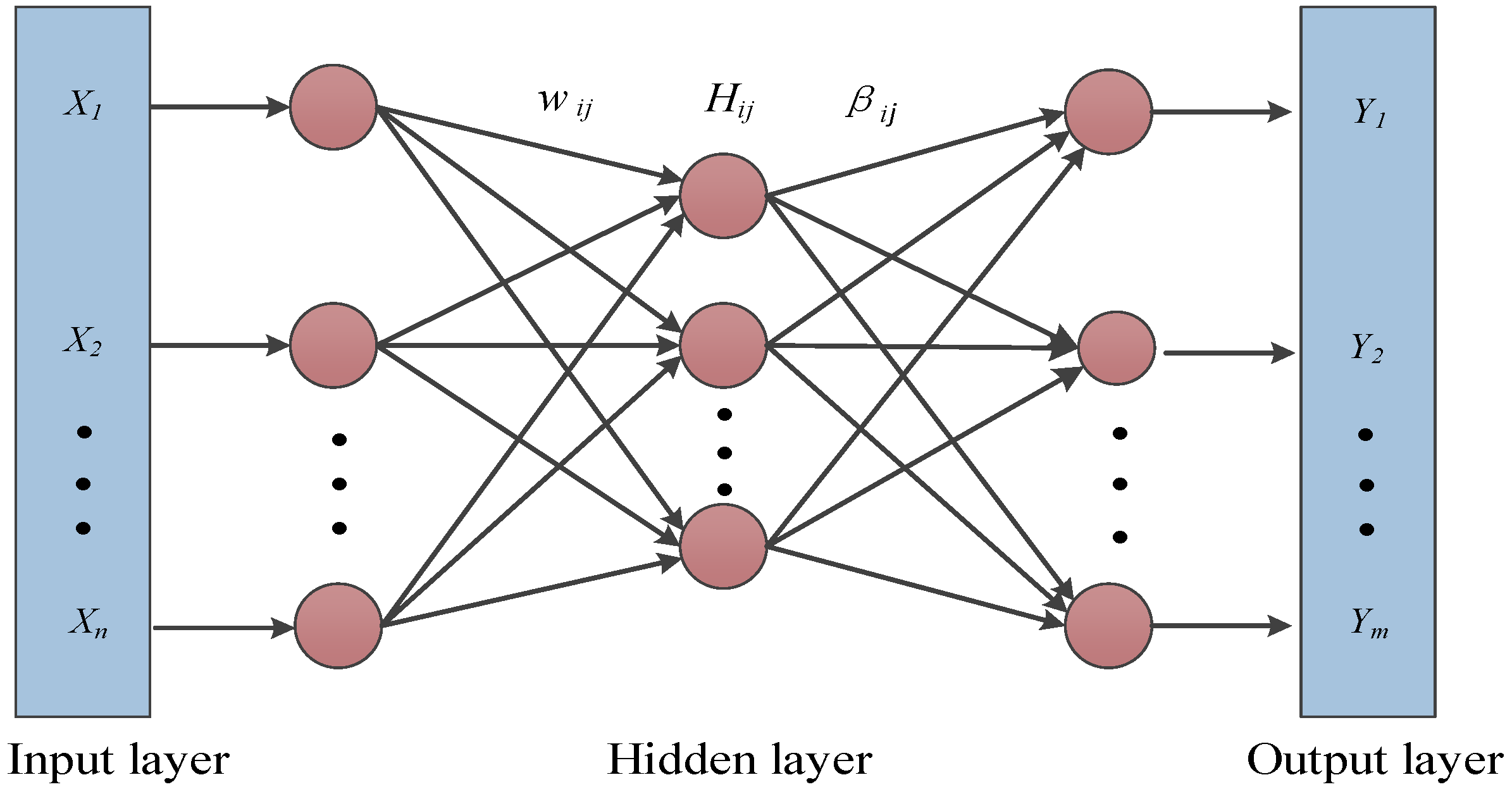
The Extreme Learning Machine (ELM) is an efficient learning architecture for Single-hidden-layer Feedforward Neural Networks (SLFNs), proposed by Huang et al. Its structural diagram is illustrated in Figure 2. Unlike traditional Backpropagation (BP) neural networks that rely on gradient descent, the core advantage of ELM lies in its non-iterative learning mechanism. By randomly mapping input weights and hidden layer biases, the algorithm transforms network training into a simple linear operator solving process, thereby significantly improving convergence speed and enhancing global optimization capability.
Let the input and output vectors of the network be denoted as x and y , respectively. If the hidden layer contains l neurons and the activation function is denoted as g ( x ) , the output matrix of the network can be expressed as:
Y = H β
Within the ELM framework, the hidden layer output matrix H carries the key information of the feature mapping. Since the activation function is typically infinitely differentiable, the input weights ω and hidden layer thresholds b can be randomly determined in advance before training and remain constant throughout the learning process. This random feature mapping greatly reduces computational complexity. Ultimately, the output layer weight matrix β can be obtained by solving the following linear least-squares problem:
min β H β Y
β ^ = H + Y
where H + represents the Moore–Penrose generalized inverse of matrix. Based on the above principles, the construction process of ELM mainly encompasses: random initialization of parameters ( ω , b), determining the hidden layer size l according to the input dimension (typically set as l = 2n + 1), calculating the output matrix H, and analytically obtaining the output weights β via generalized inverse operation.
The Twin Extreme Learning Machine (TELM) represents a structural improvement over the standard ELM, designed to handle more complex binary classification tasks. Inspired by Twin Support Vector Machines, TELM abandons the traditional approach of a single classification hyperplane and instead constructs two non-parallel hyperplanes. By solving two smaller-scale Quadratic Programming Problems (QPPs), the algorithm ensures that each hyperplane is as close as possible to its own class while maximizing the distance from the heterogeneous samples. The specific mathematical expressions for the two hyperplanes are:
f 1 x : = β 1 h x = 0 f 2 x : = β 2 h x = 0
During the solving process, the core idea of TELM is to set the objective function as the minimization of the fitting error for the samples of the current class, while setting the constraints as the suppression of the margin for heterogeneous samples. The specific QPP optimization models are formulated as follows:
min β 1 , ξ 1 2 U β 1 2 2 + c 1 e 2 T ξ subject to , V β 1 + ξ e 2 , ξ 0
min β 2 , η 1 2 V β 2 2 2 + c 2 e 1 T η subject to , U β 2 + η e 1 , η 0
where ξ and η are slack variable vectors; c1 and c2 are penalty parameters regulating structural risk and empirical risk; and e1 and e2 are vectors of all ones.
By introducing Lagrange multipliers α and γ , the above primal problems can be transformed into their corresponding Wolfe dual forms:
max α   e 2 T α 1 2 α T V U T U + ε I 1 V T α subject to , 0 α i c 1 , i = 1 , 2 , , m 2
max γ   e 2 T γ 1 2 γ T U V T U + ε I 1 U T γ subject to , 0 γ i c 2 , i = 1 , 2 , , m 2
After obtaining the optimal values of the Lagrange multipliers using an optimization algorithm, the decision variables can be determined. For any new input test sample xR, TELM determines its classification by measuring the perpendicular distance to the two decision planes:
f x = arg min d r x r = 1 , 2 = arg min r = 1 , 2 β r T h x

3. Fault Diagnosis Method

3.1. Fitness Function Design

In the process of adaptive signal decomposition, the efficacy of VMD is highly dependent on the rationality of preset parameters. Among these, the decomposition level and the penalty factor are the core variables influencing decomposition quality. The decomposition level determines the resolution of signal analysis: if set too low, under-decomposition occurs, causing signals with distinct features to be aliased within the same mode; if set too high, over-decomposition is triggered, generating false components or noise interference. The penalty factor governs the bandwidth constraint: a smaller value results in larger component bandwidths, leading to spectral overlap between modes; a larger value causes excessive bandwidth convergence, potentially resulting in the loss of critical signal features. Given the strong randomness and bias inherent in manual empirical settings, this study introduces the Improved Black-winged Kite Algorithm (IBKA) to optimize the VMD parameter combination, aiming to establish an objective and automated parameter decision mechanism. During the IBKA optimization process, it is necessary to construct an index capable of quantifying the VMD quality to serve as the fitness function. This study adopts Minimum Envelope Entropy (MEE) as the optimization objective.
Entropy is a key indicator for measuring system disorder and uncertainty, while envelope entropy can evaluate VMD quality by quantifying the sparsity of the signal. For the Intrinsic Mode Functions (IMFs) obtained via VMD, if a component contains distinct impact features (such as early mechanical fault impacts) and exhibits a low noise level, its envelope signal sequence after the Hilbert transform possesses stronger sparsity, which is mathematically reflected as a lower envelope entropy value. Conversely, if the component is filled with random noise or suffers from severe modal aliasing, the distribution of the envelope sequence tends to be uniform, leading to an increase in entropy. For a modal component u(t) of length N obtained via VMD, the calculation steps for its minimum envelope entropy are as follows:
  • Analytic Signal Construction: The Hilbert Transform is applied to u(t) to obtain its envelope signal sequence:
    a ( j ) = u ( j ) 2 + u ^ ( j ) 2 , ( j = 1 , 2 , , N )
    where u ^ ( j ) is the analytic signal of u ( j ) .
  • Sequence Normalization: To satisfy the characteristics of a probability distribution, the envelope sequence a ( j ) is normalized to obtain the probability distribution sequence P(j).
  • Envelope Entropy Calculation: According to the definition of information entropy, the envelope entropy Ep of this component is calculated as follows:
    E p = j = 1 N P ( j ) ln P ( j )
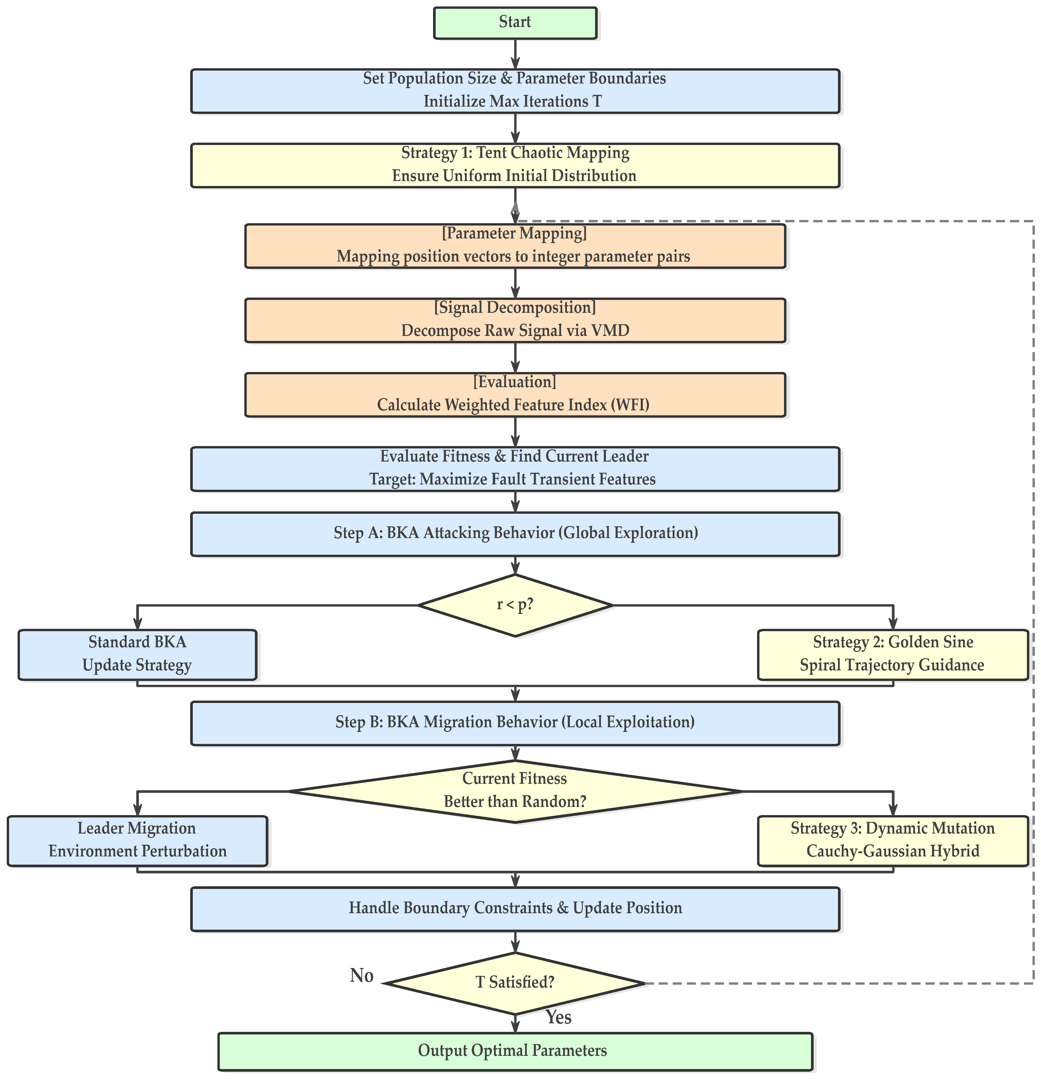
In the IBKA, since VMD decomposes the signal into multiple components, to ensure the overall decomposition result is optimal, this study selects the minimum envelope entropy value among all IMF components as the current fitness value. The main workflow for optimizing VMD parameters using IBKA is illustrated in Figure 3, with the basic steps described as follows:
  • Population Initialization and Strategy Deployment: First, the improved strategies of the IBKA are utilized to generate an initial population within the preset parameter space. Each individual represents a set of parameter combinations to be optimized, and a rounding operator is employed to realize the logical mapping from the continuous search space to the integer parameter space.
  • Signal Decomposition and Evaluation: The mapped parameters are input into the VMD algorithm to decompose the original signal. For the obtained modal components, their envelope entropy indicators are extracted sequentially to quantitatively evaluate the manifestation degree of fault impact features under the current parameters.
  • Fitness Feedback and Optimization Iteration: Following the “Best Component Criterion,” the minimum envelope entropy value among the k signal components is selected as the fitness function and fed back to the IBKA. Based on the fitness value, the algorithm dynamically adjusts the search step size and direction using its unique search mechanism, guiding the population to evolve toward the region where the fitness function is minimized.
  • Optimal Result Output: When the algorithm reaches the preset termination criterion or converges to a stable value, the iteration stops. The globally optimal parameter combination is output and used as the final basis for decomposition, thereby achieving the decoupling of bearing fault signals.

3.2. Optimal IMF Component Selection Strategy

After processing bearing vibration signals via VMD, the signals are decomposed into a series of Intrinsic Mode Functions (IMFs) in the time-frequency domain. However, as an over-complete decomposition method, VMD inevitably generates redundant modes or spurious components dominated by noise under strong noise backgrounds. If all IMFs are blindly superimposed for signal reconstruction, broadband random noise will severely obscure weak fault impact features, leading to a degradation in feature extraction accuracy. To address this limitation, this study proposes an adaptive screening mechanism based on the principle of Statistical Significance. The core mechanism lies in accurately extracting modes containing core fault dynamics by quantifying the “prominence” of component feature strength within the overall distribution. The design rationale utilizes the Squared Envelope Spectrum Gini Index (SESGI) to characterize the sparsity of signal energy distribution, while simultaneously capturing the impulse intensity of periodic impacts via the Squared Envelope Spectrum Kurtosis (SESK).
(1)
Extraction of the Squared Envelope Spectrum (SES): For the i-th IMF μ i ( t ) , obtained via VMD, the Hilbert transform is first applied to calculate its squared envelope signal e i ( t ) to eliminate the influence of carrier frequencies and highlight low-frequency impact features:
e i ( t ) = u i ( t ) + j H u i ( t ) 2 E ¯
where H denotes the Hilbert transform, and E ¯ represents the removal of the direct current component. A Fast Fourier Transform (FFT) is then applied to e i ( t ) to obtain the squared envelope spectrum P i ( f ) . To eliminate the influence of energy amplitude on the evaluation results, the spectrum is normalized:
P n o r m ( k ) = P i ( k ) k = 1 M P i ( k )
where M represents the number of spectral sampling points, and P i ( k ) is the amplitude of the i-th component at the k-th frequency point.
(2)
Squared Envelope Spectrum Kurtosis (SESK): Kurtosis is a fourth-order cumulant reflecting the distribution characteristics of a signal. Calculating SESK in the frequency domain effectively characterizes the prominence of characteristic frequencies and their harmonics in the envelope spectrum. It is defined as:
S E S K = E ( P n o r m μ p ) 4 σ p 4
where E denotes the mathematical expectation operator; μ p represents the mean of the normalized spectral sequence; and σ p represents the standard deviation of the sequence P n o r m .
(3)
Squared Envelope Spectrum Gini Index (SESGI): The Gini index was originally used in economics to measure inequality and has recently been introduced into signal processing to evaluate signal sparsity. Compared to kurtosis, SESGI exhibits better robustness against random noise and singular points. The calculation involves arranging the M elements of the normalized spectrum P n o r m in ascending order as a sequence P ^ 1 , P ^ 2 , , P ^ M . The formula is as follows:
S E S G I = 1 2 k = 1 M P ^ k P n o r m 1 ( M j + 0.5 M )
where P n o r m 1 represents the L1-norm of the sequence, and P ^ k denotes the value of the k-th element in the sorted sequence.
To balance the sensitivity of SESK and the robustness of SESGI, this study defines the Weighted Feature Indicator (WFI) using a weighted product approach. To prevent the SESK value from becoming excessively large and dominating the evaluation, a logarithmic non-linear mapping is applied. The comprehensive score for the i-th IMF is defined as:
W F I i = S E S G I i log 10 ( 1 + S E S K i )
This study utilizes the Weighted Feature Indicator (WFI) to conduct a multi-dimensional quality assessment of the k modal components. The WFI organically combines the sparse representation capability of the Squared Envelope Spectrum Gini Index (SESGI) for signal energy distribution with the high sensitivity of the Squared Envelope Spectrum Kurtosis (SESK) to transient impacts. From a physical mechanism perspective, IMFs containing fault information should exhibit energy concentration in the frequency domain and significant periodic impulse characteristics in the time domain.
To establish a dynamic baseline for distinguishing “effective signals” from “background noise,” the first-order statistic (mean μ W F I ) and second-order statistic (standard deviation σ W F I ) of the score sequences for all IMF signal components are calculated:
μ W F I = 1 k i = 1 k W F I i
σ W F I = 1 k i = 1 k ( W F I i μ W F I ) 2
where μ W F I represents the “average performance” of the feature strength of each signal component under the current decomposition state, while σ W F I reflects the degree of dispersion of feature strength among the components. In complex noise backgrounds, if a component carries genuine fault information, its WFI value, acting as an anomalous statistic, should significantly deviate from the mean center as an “outlier.” This degree of deviation constitutes the core basis for screening.
To achieve adaptive noise isolation, a dynamic threshold T is constructed:
T = μ W F I + γ σ W F I
where γ is a proportional adjustment factor (empirically set to 0.8 in this study) used to balance the sensitivity of feature extraction with the robustness of noise reduction. The physical implication of this threshold is to delineate a statistically significant “prominence interval.” Only when the feature score of an IMF component crosses this boundary is it considered a candidate component containing effective dynamic responses.
After obtaining the candidate signal components, to further ensure the purity of the reconstructed signal, a hard constraint strategy based on the survival-of-the-fittest mechanism is implemented:
  • Rank Sorting and Preferential Selection: All components passing the threshold T are sorted in descending order based on their WFI values. This procedure aims to prioritize modes with the most concentrated energy and the clearest fault pulses, ensuring that the reconstruction process is driven by dominant features.
  • Capacity Hard Constraint: Considering that the resonance response induced by bearing faults is typically confined to specific frequency bands, the maximum number of retained components is set to 3 in this study. This constraint effectively blocks potential interference modes from entering the reconstruction stage. In exceptional cases where no component exceeds the threshold, the mode corresponding to the maximum WFI value is forcibly selected to ensure the continuity of the diagnostic logic.
  • Signal Reconstruction: The index set of the finally selected modes defines the constituent components of the reconstructed signal. The final reconstructed signal is formed by the linear superposition of the components within this set.
Through the progressive screening process—ranging from statistical benchmarks to capacity constraints—the system is able to “extract” high-SNR (Signal-to-Noise Ratio) feature components from the cluttered decomposition results, thereby laying a solid foundation for subsequent precise feature identification.

3.3. Implementation Process of Improved Transformer-TELM Model

The specific implementation steps of the proposed fault diagnosis method are detailed as follows:
(1)
Adaptive Optimization of VMD Key Parameters: To overcome the stochasticity and subjectivity inherent in manual parameter tuning, the IBKA is introduced to perform a global search within the VMD parameter space. In this process, Envelope Entropy is designated as the objective function. By minimizing the value of this function, the algorithm is driven to adaptively iterate and identify the parameter configuration that most clearly reveals fault impact features, thereby ensuring optimal VMD performance in subsequent decomposition tasks.
(2)
Variational Mode Decomposition and Component Screening: The raw vibration signal acquired from the rolling bearing is utilized as the input. The pre-optimized VMD model is applied to decompose the signal into a series of IMFs. Subsequently, the Squared Envelope Spectrum (SES) is computed for each component to extract the SESK and SESGI. A dynamic threshold screening strategy is employed to synthesize a comprehensive WFI score, which is used to quantitatively evaluate the richness of fault features in each component. Finally, the modal indices are selected based on the WFI scores, and a reconstructed signal with suppressed noise and enhanced features is constructed via linear superposition of the selected modes.
(3)
Mapping and Representation of the Initial Feature Space: For the reconstructed signal, the HFrAttE feature vector is calculated. This feature extraction method organically integrates the sensitivity of fractional-order entropy in capturing subtle nonlinear variations with the multi-band resolution capability of hierarchical decomposition, thereby providing a high-quality input source for the subsequent deep learning stage.
(4)
Deep Feature Evolution Based on Improved Transformer: The HFrAttE feature vector is input into the improved Transformer model. The model automatically identifies and aggregates complex patterns hidden within the data, transforming the low-dimensional initial entropy features into deep feature representations that are more robust and conducive to classification.
(5)
Fault Diagnosis: The deep discriminative features extracted in the preceding steps are utilized as the input for the TELM classifier. By leveraging the characteristic of TELM that delineates decision boundaries through the solution of two non-parallel hyperplanes, a rapid mapping of the bearing operating conditions is achieved, completing the fault diagnosis process.

4. Experimental Verification

4.1. Performance Evaluation of the IBKA

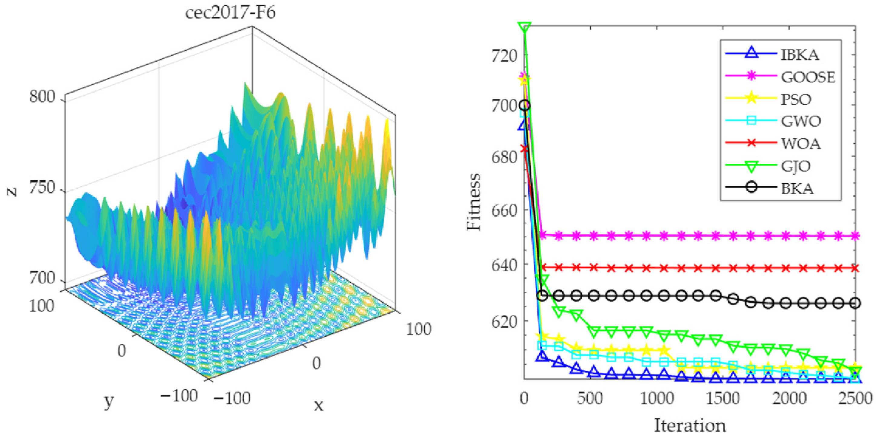
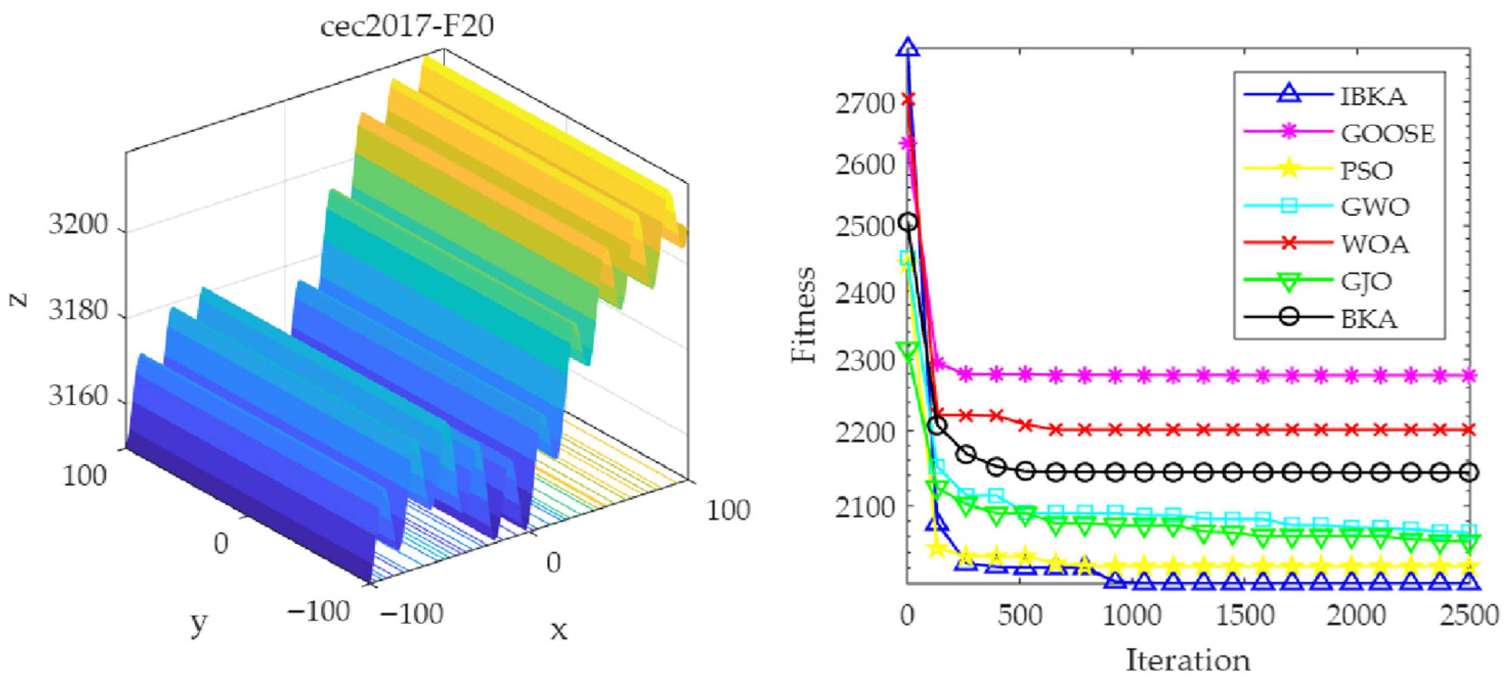
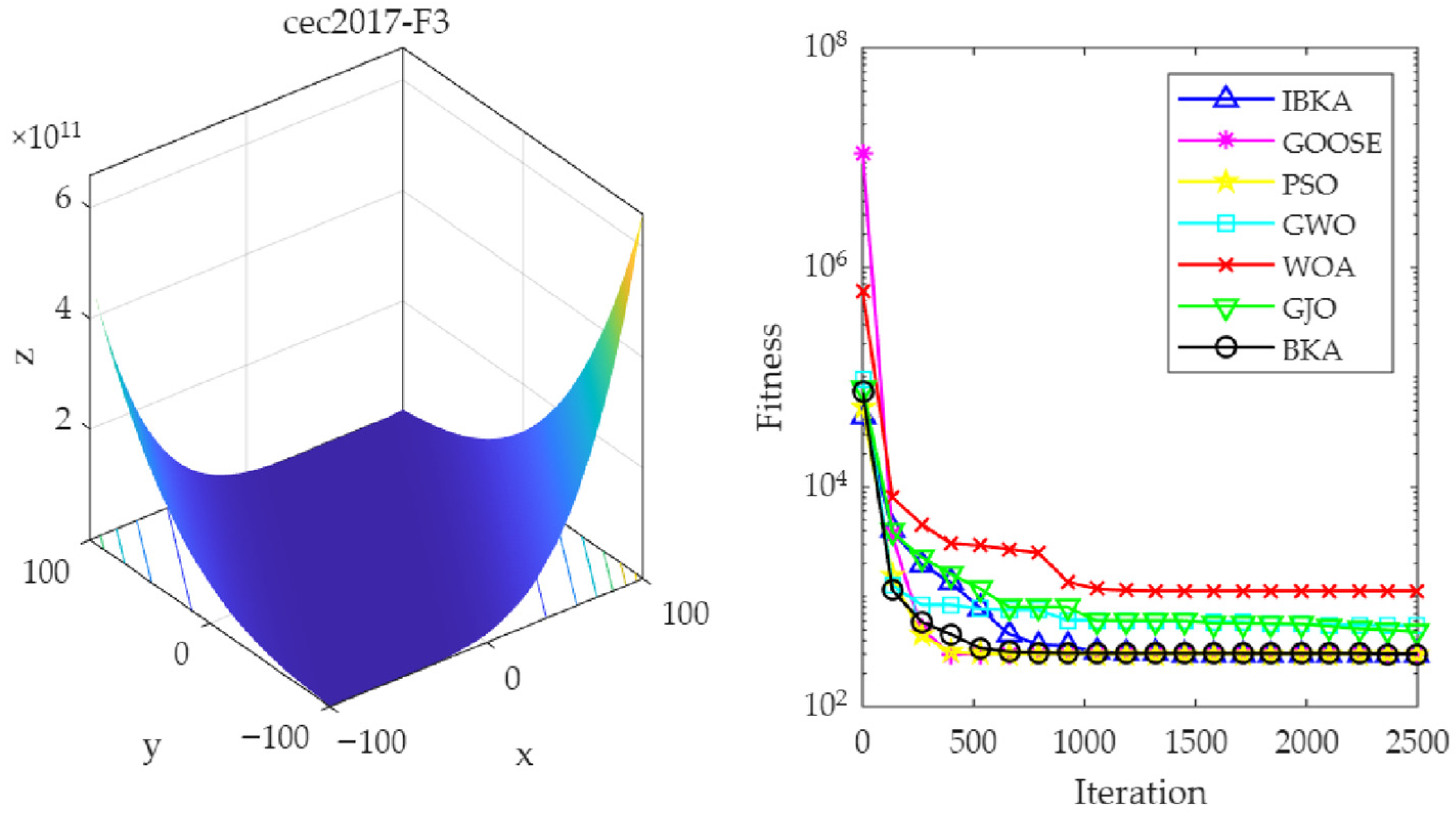
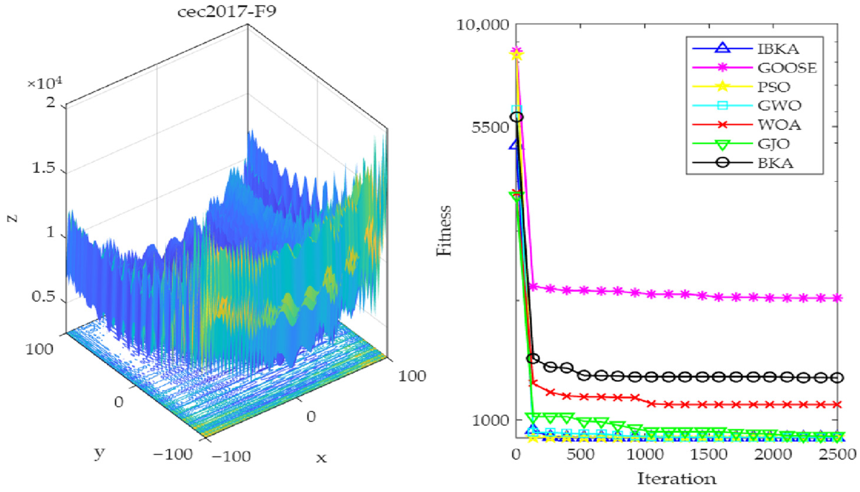
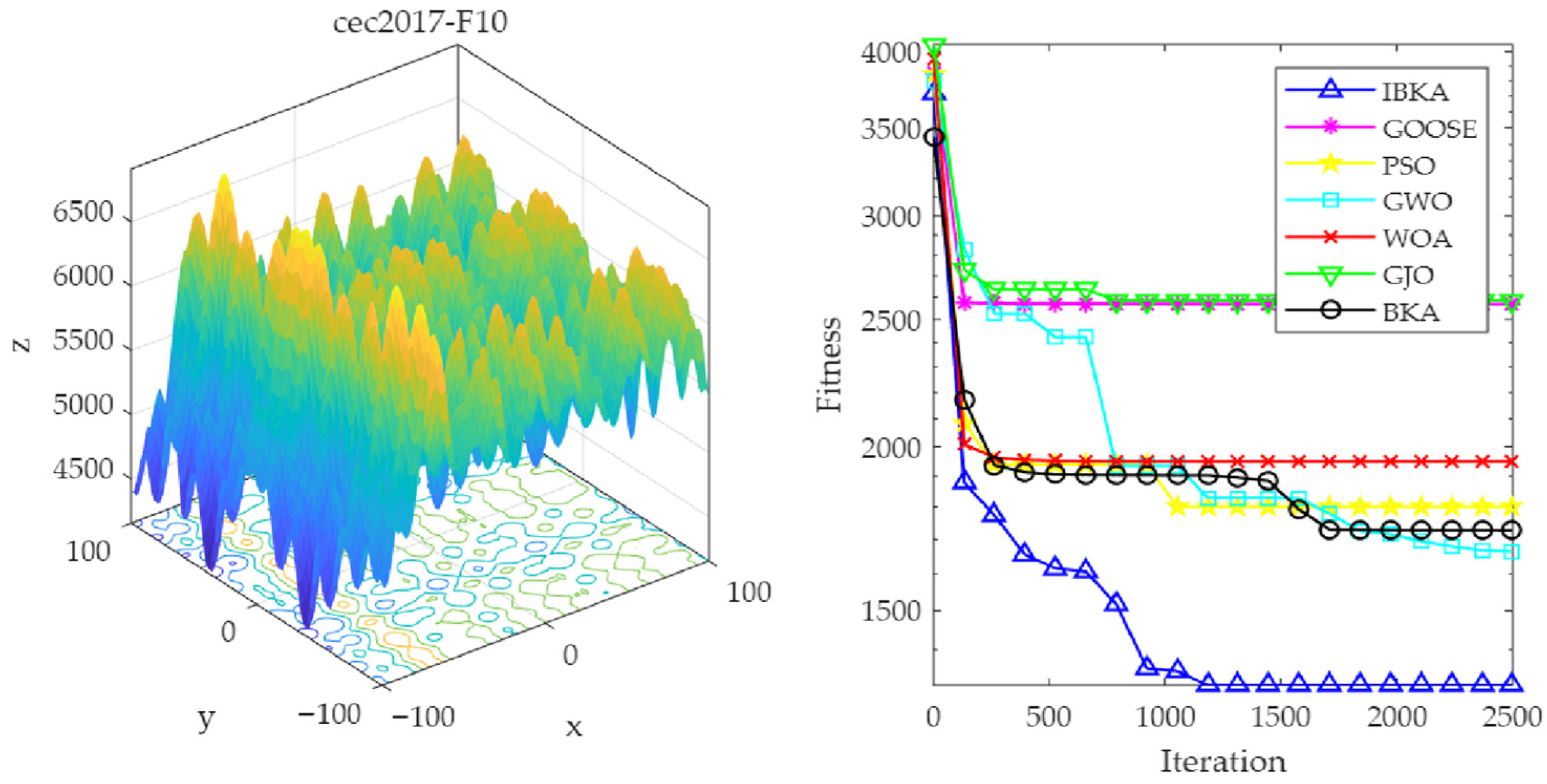
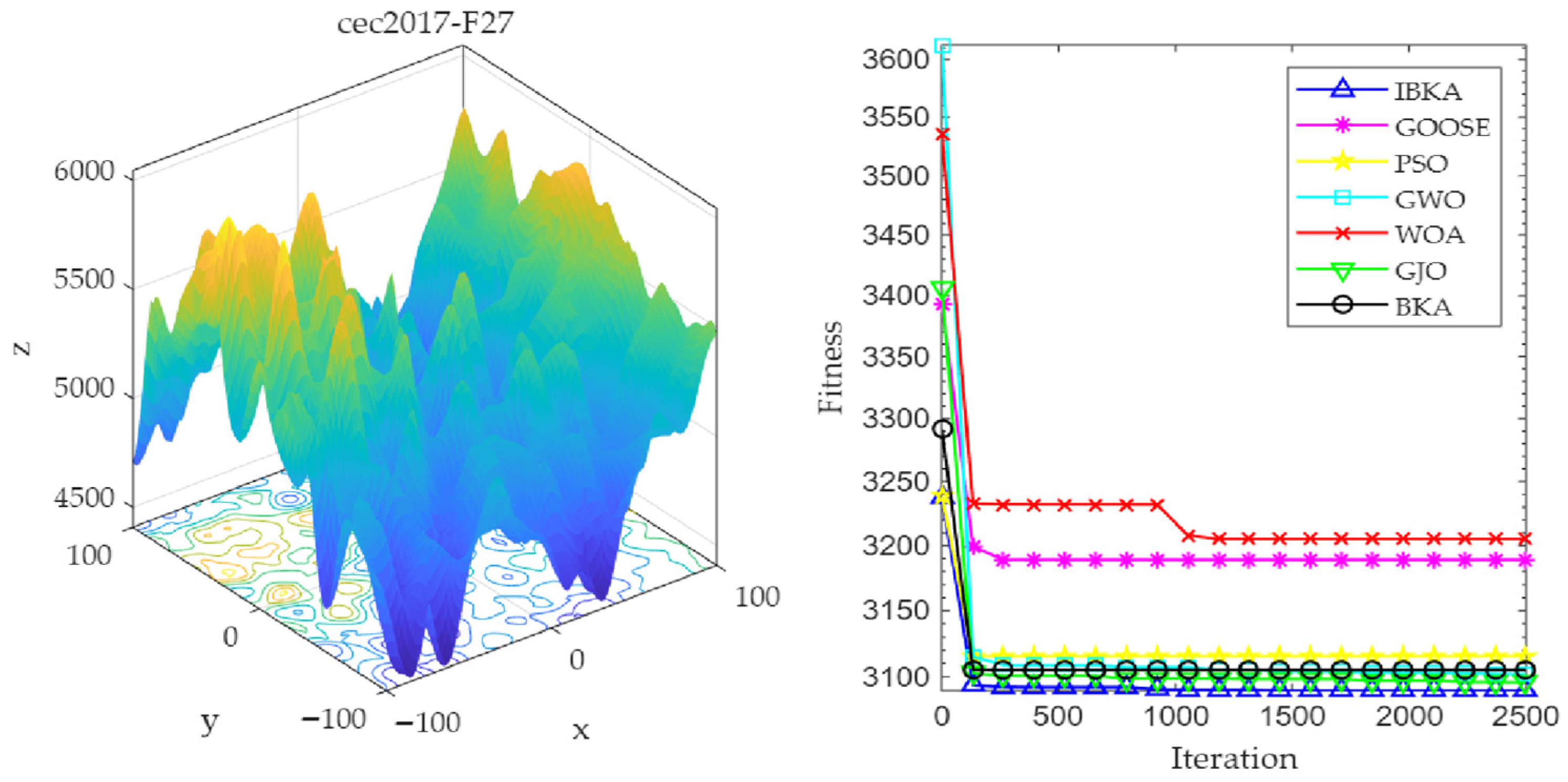
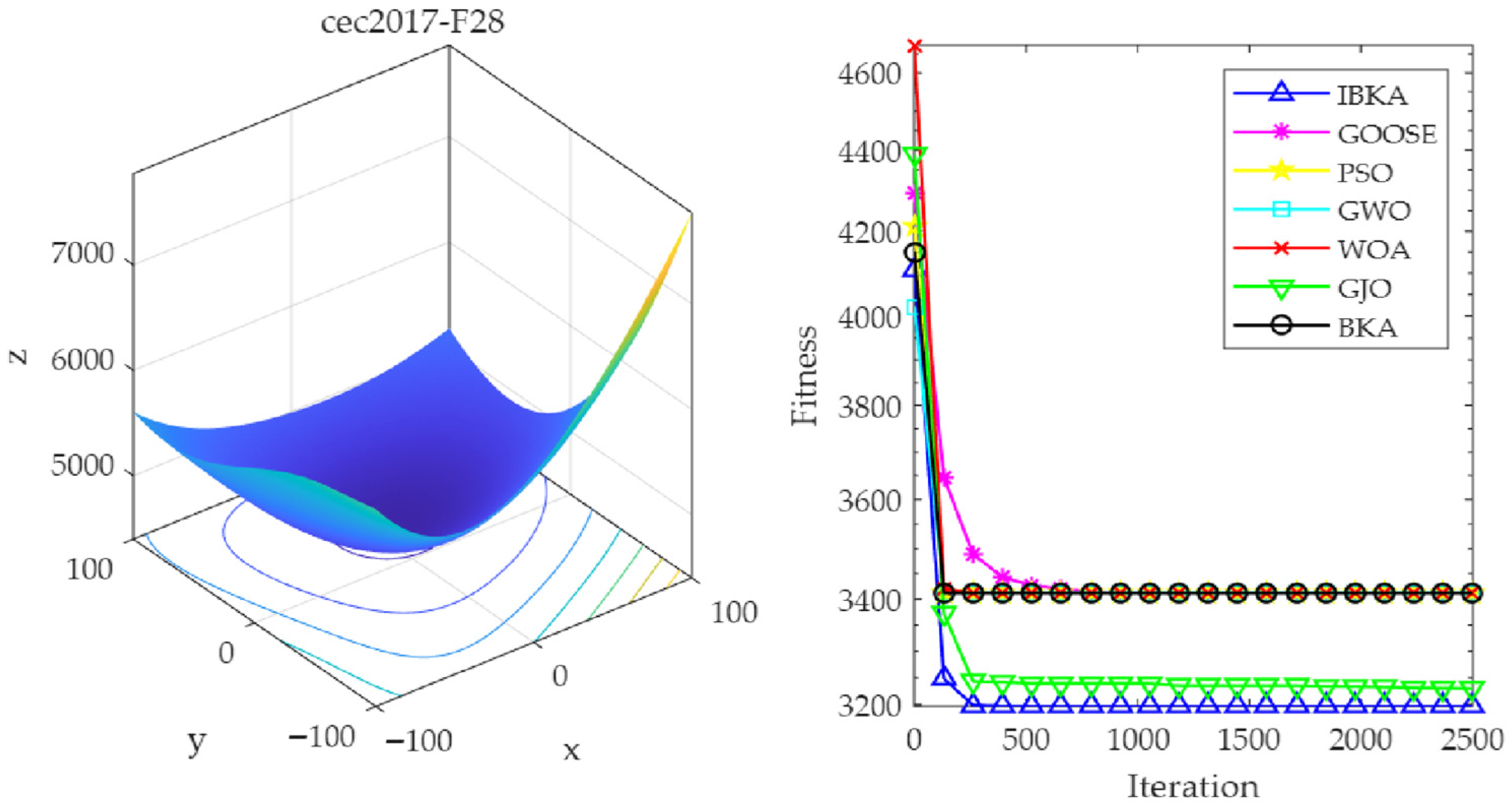
To comprehensively evaluate the practical efficacy of the IBKA in solving complex optimization problems, a systematic comparative testing framework was constructed. A variety of representative algorithms were introduced as reference benchmarks, aiming to cover different evolutionary stages of heuristic search. These benchmarks include classical algorithms such as Particle Swarm Optimization (PSO) and the original BKA, as well as high-performance operators that have been active in academia in recent years, such as the GOOSE Algorithm (GOOSE), Grey Wolf Optimizer (GWO), Whale Optimization Algorithm (WOA), and Golden Jackal Optimization (GJO). Regarding the selection of the test environment, the CEC2017 benchmark suite, released by the IEEE Congress on Evolutionary Computation, was adopted. This suite is regarded as the “gold standard” for algorithm performance evaluation because its integrated mathematical functions cover scenarios ranging from unimodal to multimodal, and even highly nonlinear composite functions. To ensure the pertinence of the tests, eight challenging functions (F3, F6, F9, F10, F20, F25, F27, F28) were selected for focused analysis. The complex topological structures of these functions effectively test an algorithm’s ability to escape local optima.
Convergence efficiency and solution accuracy are the core metrics for measuring algorithm performance. Consequently, the fitness evolution curves of the comparative algorithms during the iteration process were recorded in detail and plotted (see Figure 4, Figure 5, Figure 6, Figure 7, Figure 8, Figure 9 and Figure 10). By horizontally comparing the descent gradients and stability characteristics of these curves, the following phenomena were observed: In the early stage of evolution, the fitness curve of IBKA exhibited a significant vertical descent trend. This demonstrates that the improvement strategies introduced in this paper effectively expand the effective search space of the population, enabling the algorithm to rapidly lock onto high-probability solution regions in the initial phase.
Furthermore, IBKA demonstrated superior robustness, particularly when handling functions such as F6 and F10. Unlike other algorithms that suffer from premature convergence, the improved mechanism of IBKA guides the population to continuously approximate the global optimum. The experimental results indicate that IBKA not only possesses advantages in convergence speed but also achieves a lower mean fitness value compared to other peer algorithms.
To enhance the credibility and robustness of the experimental results, a series of repetitive experiments were conducted under strictly controlled conditions. Regarding the experimental configuration, the algorithm population size was fixed at 30 individuals, and the maximum number of iterations was set to 2500. For each comparative algorithm, 30 independent runs were executed. By averaging the results of multiple independent runs, the stochastic influence introduced by single executions was effectively mitigated, allowing for a more precise assessment of the algorithms’ true performance.
Upon completion of the experiments, the data from each run were processed to calculate and record the Standard Deviation (Std), Average (Avg), and Median. These metrics were utilized as key quantitative indicators for evaluating the optimization performance of the algorithms; the specific data are presented in Table 1. Specifically, the standard deviation measures the dispersion of the data, reflecting the fluctuation of results across multiple runs; the average represents the central tendency, demonstrating the overall optimization level; and the median provides a more robust reflection of the intermediate data level.
Through a detailed examination and comparative analysis of the data in Table 1, it is evident that the IBKA demonstrated superior performance on functions F10, F27, and F28 compared to the other optimization algorithms. Across the three dimensions of Std, Avg, and Med, the IBKA consistently outperformed the other algorithms. This is attributed to the Cauchy Gaussian dynamic mixture mutation mechanism: in the later stages of iteration, the non-linear rapid descent of λ accelerates the transition to Gaussian mutation, thereby achieving extremely high optimization accuracy in the complex ridge space of the mixture function.
For unimodal or multimodal functions such as F3, F6, F9, and F20, although IBKA exhibits a “slightly inferior” performance numerically (e.g., its mean value (Ave) for F3 matches that of the optimal algorithm, but there is a certain deviation in the standard deviation (Std)), or performs on par with a few other algorithms, these minor precision fluctuations represent necessary trade-offs made by the algorithm to maintain global search robustness when addressing complex multimodal problems. Overall, its metric values remain at a relatively high level. Given that bearing fault diagnosis in practical engineering often involves highly complex search spaces with numerous traps, IBKA’s advantages on these functions demonstrate its stronger practical value in solving real-world industrial problems.

4.2. Bearing Fault Diagnosis Experimental Analysis

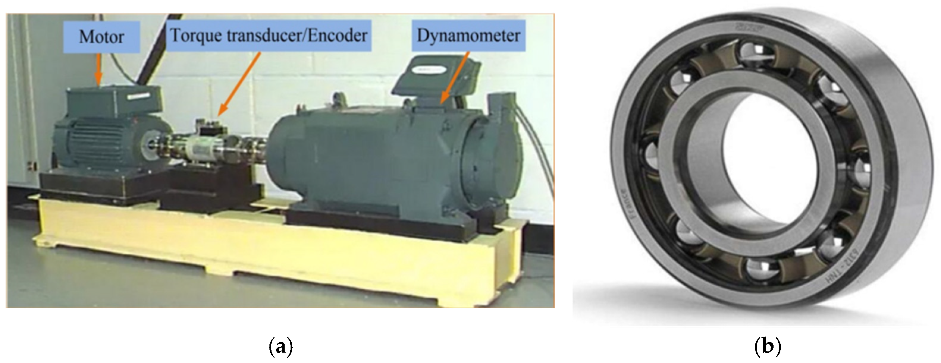
To rigorously evaluate the robustness and practical value of the proposed algorithm, the authoritative Case Western Reserve University (CWRU) bearing public dataset was introduced. The test platform structure supporting the generation of this dataset is illustrated in Figure 11 [31,32,33]. The precise integration of its power system, sensing units, and power monitoring modules establishes the physical foundation for capturing high-quality fault signals. During the experimental phase, SKF 6205 components were selected as the research subject. Subtle single-point damages were pre-fabricated on the inner race, rolling elements, and outer race utilizing precision Electrical Discharge Machining technology. This process highly reproduces the fatigue evolution process observed in industrial scenarios. In the data acquisition stage, the system sampling frequency was configured to 12 kHz. Coupled with a constant motor speed of approximately 1800 r/min, vibration data corresponding to a fault size of 0.007 inches were specifically extracted. This ensures that the subsequent diagnostic model can acquire raw fault representations rich in time-frequency features.
In the preprocessing of the acquired raw signals, a shifted window mechanism with overlapping features was introduced to enhance the coherence of feature representation through temporal redundancy. Regarding the specific configuration parameters, the coverage length of the sampling window was set to 2048 discrete data points, while the step displacement between adjacent windows was confirmed as 1000 points. Based on this sampling strategy, for the healthy operating state and three typical preset damage types, 120 feature samples were extracted for each category, thereby constructing a dataset comprising 480 valid samples.
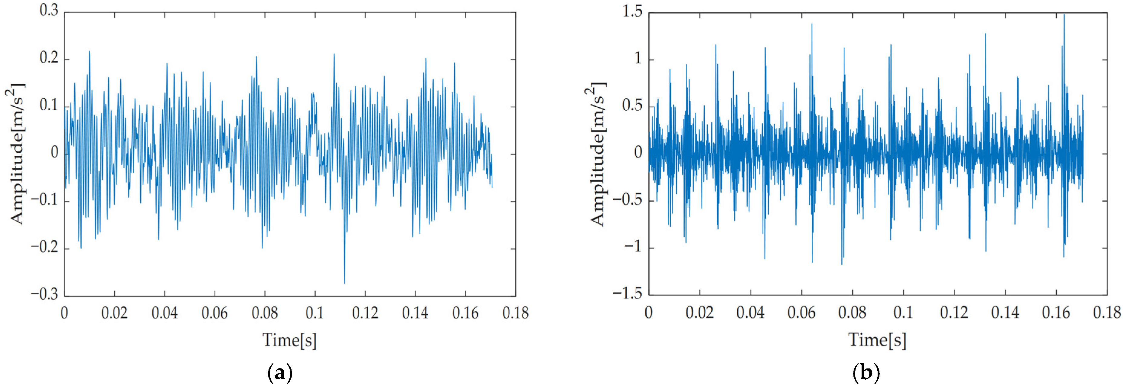
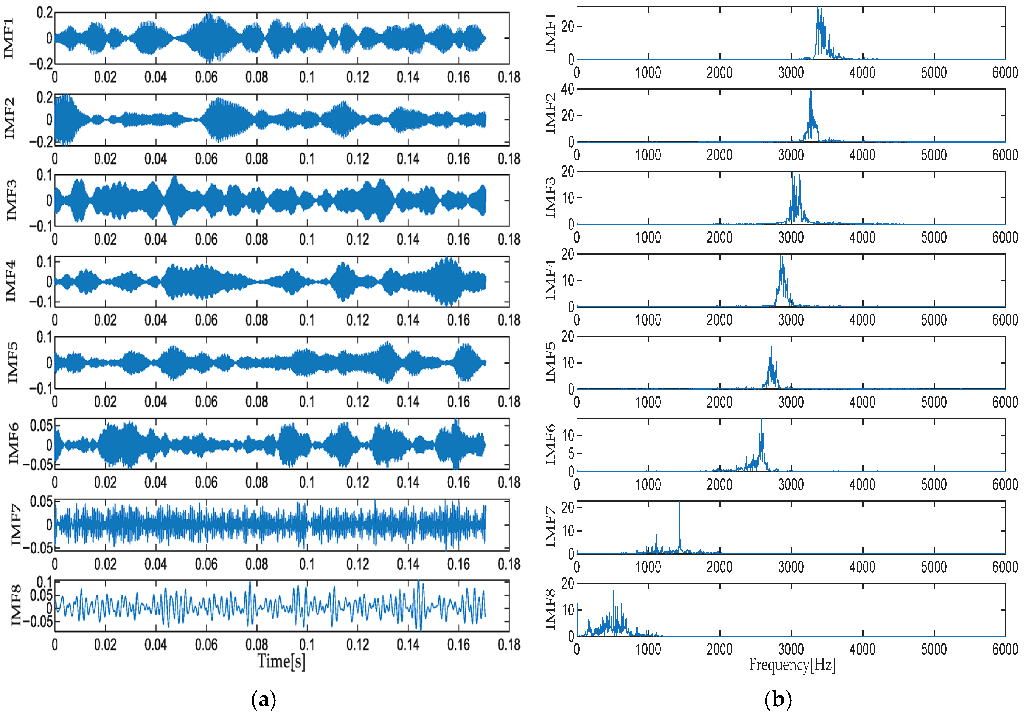
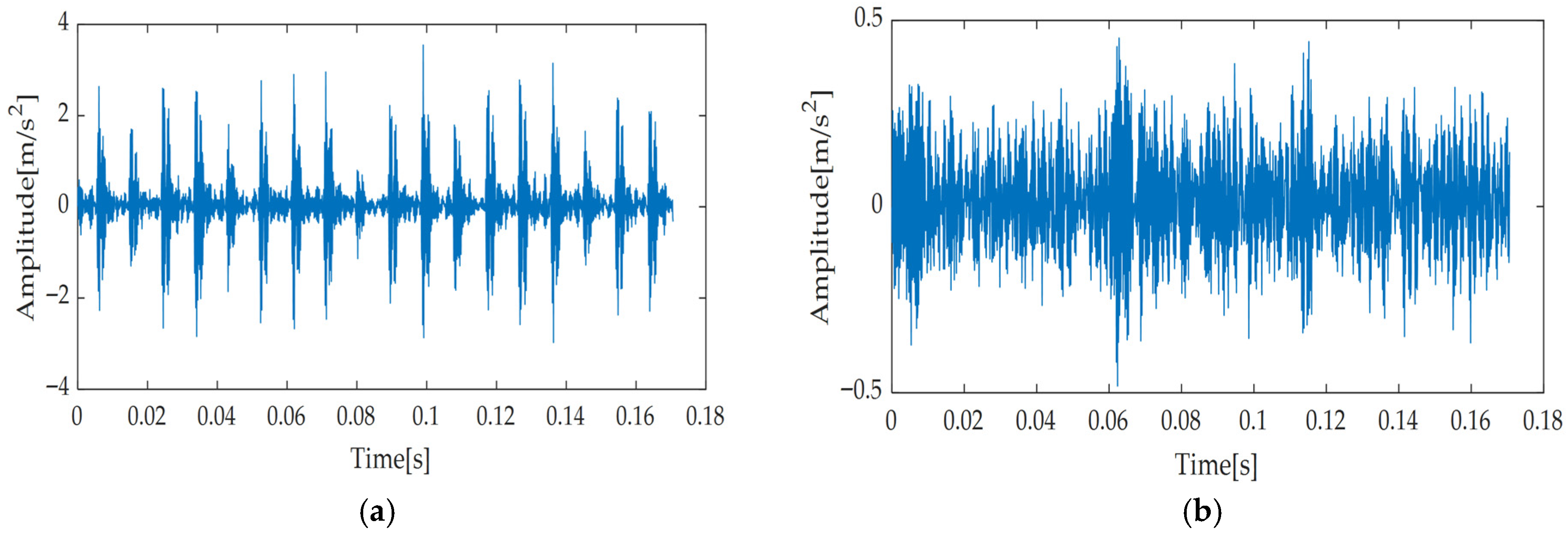
For the subsequent evaluation protocol design, the sample set was partitioned into two subsets with a scale ratio of 75% and 25%. This asymmetric allocation mode not only ensures that the classifier can learn sufficient discriminative features but also guarantees the objectivity and generalization reference value of the final performance testing. The time-domain waveforms and spectrum diagrams of the bearing under different operating states extracted during the experiment are presented in Figure 12 and Figure 13.
To further verify the reliability of the proposed algorithm in complex acoustic environments, noise with signal-to-noise ratios (SNRs) of −2 dB and −5 dB was introduced into the raw signals of four bearing operating conditions. This testing protocol is designed to faithfully reproduce the complex and variable background interference encountered in industrial settings. By analyzing the response to varying noise intensities, a basis is provided for evaluating the robustness and anti-interference potential of the diagnostic model.
In the initial experimental phase, the constructed parameter optimization program was utilized to drive the IBKA to adaptively match the core parameters within VMD. To accurately characterize the decomposition efficacy of the signal, Envelope Entropy was introduced as the discrimination criterion. This metric enables an objective evaluation of the extraction quality of fault impact components by VMD through the quantification of the vibration signal’s sparsity. During the iterative optimization process, the minimum value of the envelope entropy of each component after VMD was extracted as the fitness function and fed back to the IBKA model. Leveraging its unique spatial exploration mechanism, the algorithm dynamically regulates the evolutionary step size, guiding the population to converge toward the minimization space of the objective function. The specific search dimensions were configured as follows: the decomposition level was constrained within the range of 3 to 9, and the penalty factor was restricted to the interval of 100 to 3000. Concurrently, the IBKA population size was set to 30, and the maximum number of iterations was set to 20 to balance search completeness with computational efficiency.
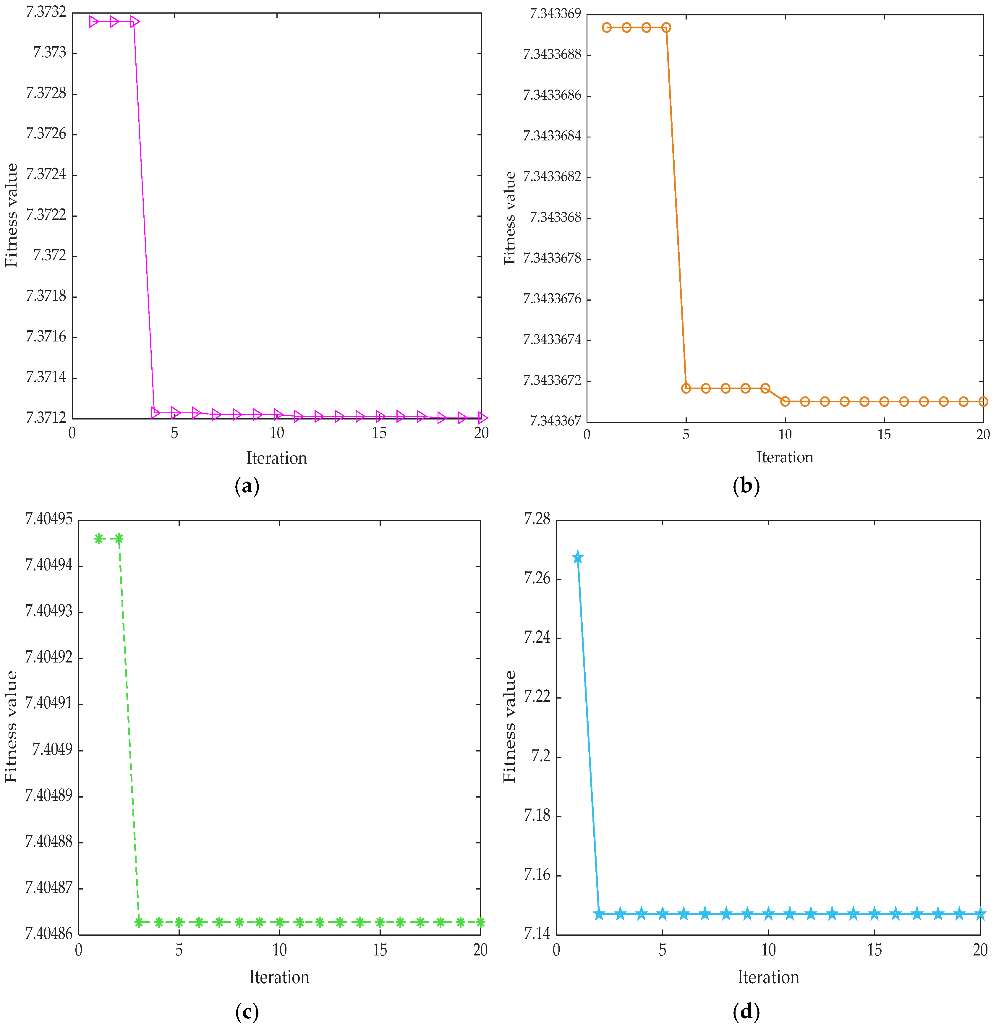
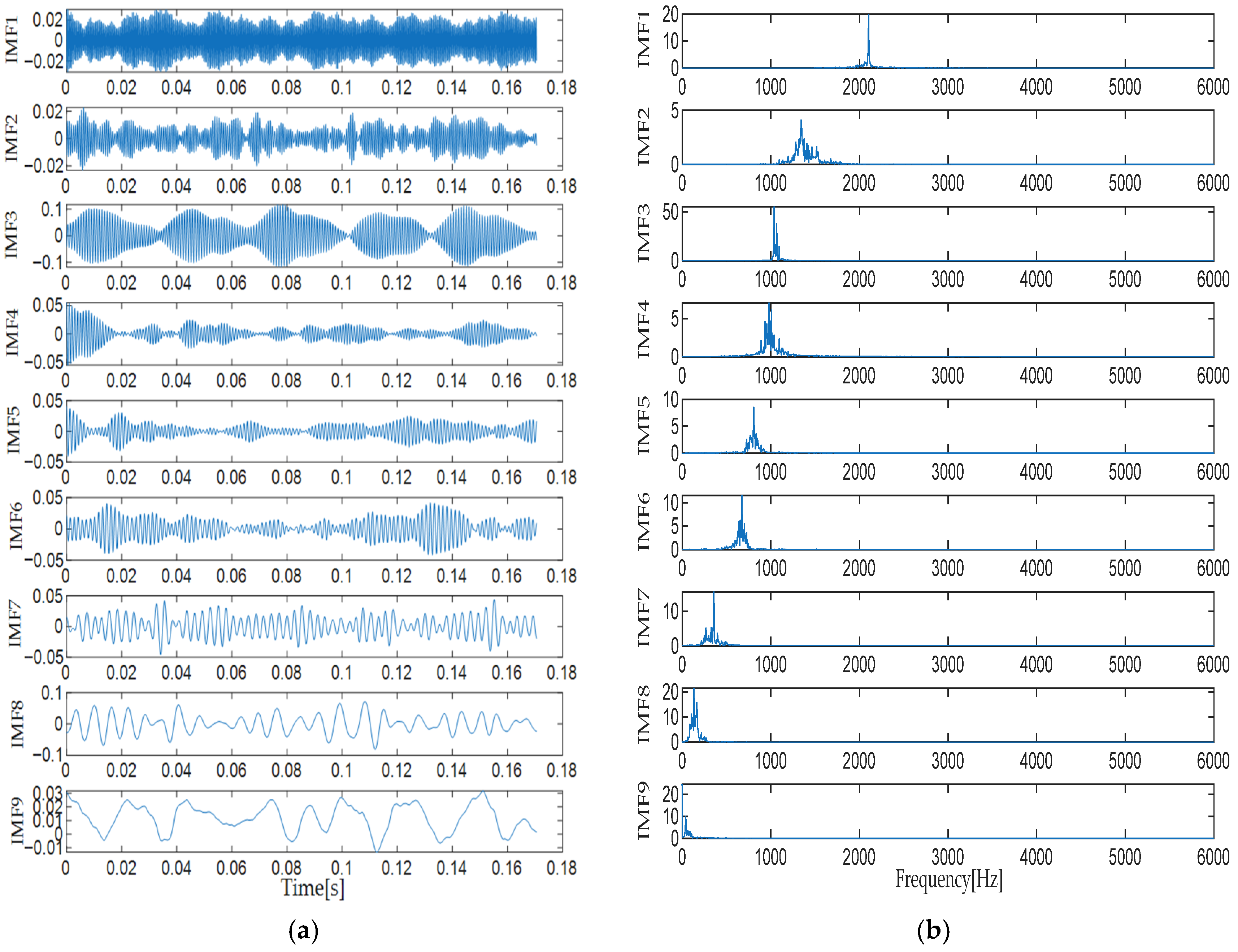
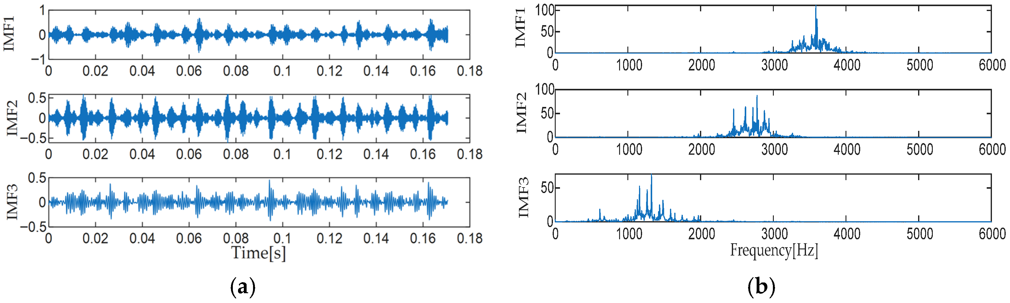
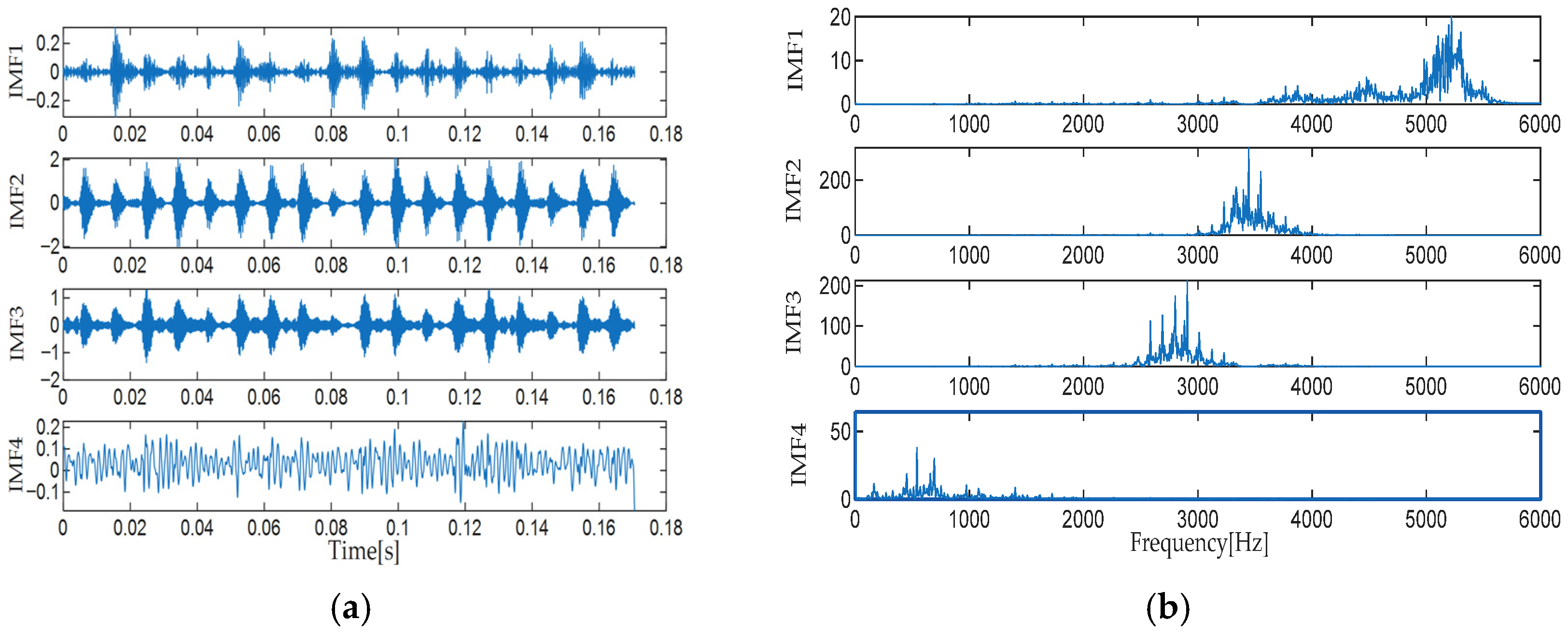
Due to space limitations, the experimental results for the noise-free data group are presented below as an example. Upon completion of the optimization process, Figure 14 illustrates the evolutionary trajectories of the fitness curves under four typical operating conditions (including healthy, inner race defect, outer race defect, and rolling element defect states). The statistical results of the optimal solutions under different noise levels are presented in Table 2. It can be observed that the algorithm exhibits a rapid convergence speed. When the fitness reaches the optimal state, distinct differences are observed in the values of the decomposition level k and penalty factor α for the rolling bearing across different operating conditions. For example, under the condition of no added noise, when the bearing operates normally, the value of α is 2303 and the value of k is 9; when there is an inner race fault, the value of α is 2840 and the value of k is 3; when there is an outer ring fault, the value of k is 100 and the value of α is 4; and when there is a rolling element fault, the value of α is 3000 and the value of k is 8. Based on these optimization results, the determined optimal parameter set was substituted into the VMD model to decompose the bearing signals. The time-frequency analysis results in Figure 15, Figure 16, Figure 17 and Figure 18 confirm that the optimized VMD algorithm significantly suppresses the mode aliasing effect, achieving an effective decoupling of high-frequency noise and low-frequency fault primitives in the signal. This high-fidelity signal reconstruction provides reliable data support for subsequent feature extraction and fault identification.
After being processed by VMD, the raw vibration signal is mapped into a set of IMFs possessing specific physical significance. To objectively measure the feature contribution of each component, a Weighted Feature Indicator (WFI) is defined as the algorithm’s discrimination criterion, enabling a multi-dimensional quality assessment of the decomposed IMFs. This indicator synergistically integrates the SESGI, which characterizes the sparse distribution of energy efficiency, and the SESK, which reflects the transient impact characteristics of impulses.
Furthermore, to precisely isolate effective fault features under complex operating conditions, a dynamic thresholding strategy based on statistical distribution laws is constructed. This threshold utilizes the first-order statistic (mean, μ W F I ) and the second-order statistic (standard deviation, σ W F I ) of the entire modal score sequence as benchmarks, establishing a criterion to distinguish information components from noise interference. Consequently, adaptive screening of the optimal modes is achieved.
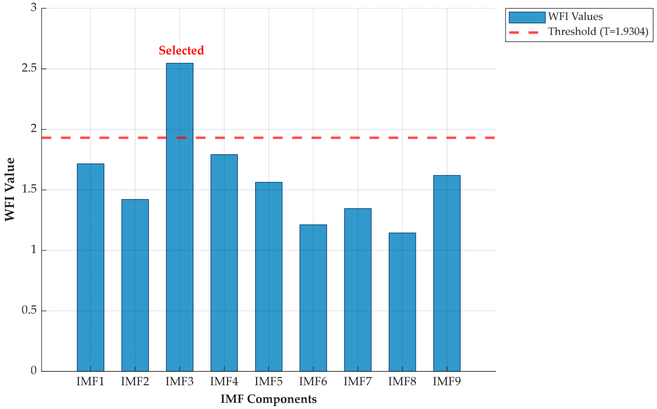
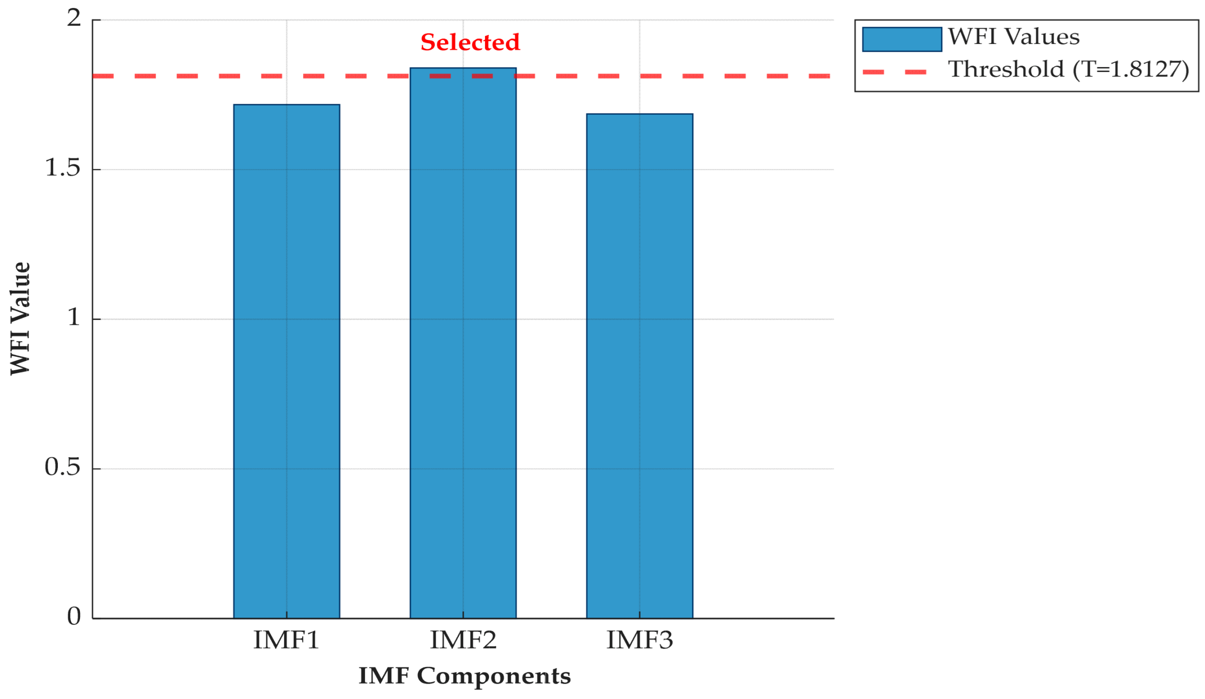
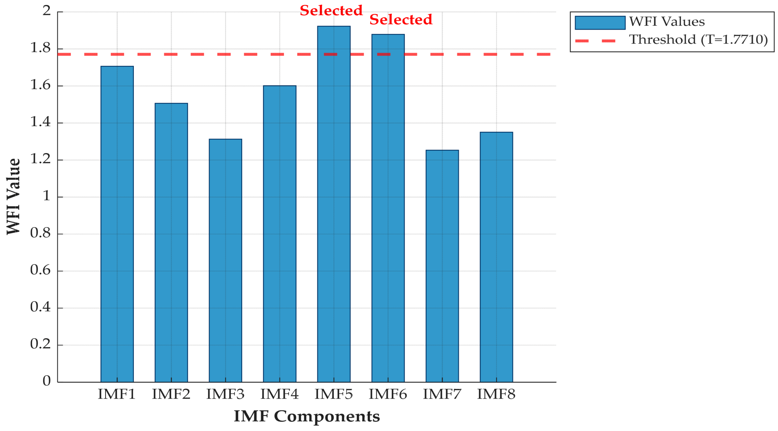
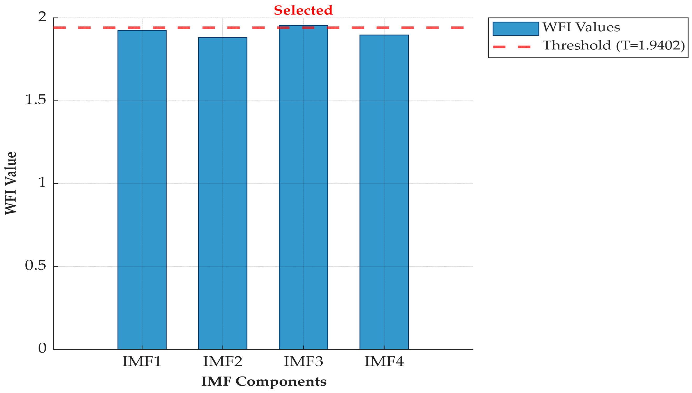
Figure 19, Figure 20, Figure 21 and Figure 22 intuitively reveal the evolutionary trends of the WFI for each IMF component under four typical operating conditions, derived from a set of data analyses (noise-free group). By observing the intersection characteristics between the curves and the threshold line, the following patterns are identified: when the bearing is in a healthy state, the optimal signal component is IMF3; when an inner race fault occurs, the optimal component is IMF2; if a rolling element fault is present, the optimal components are IMF5 and IMF6; and when an outer race fault occurs, the optimal component is IMF3. Based on the analysis results of these four states, a signal reconstruction operation is performed on the selected IMF signal components.
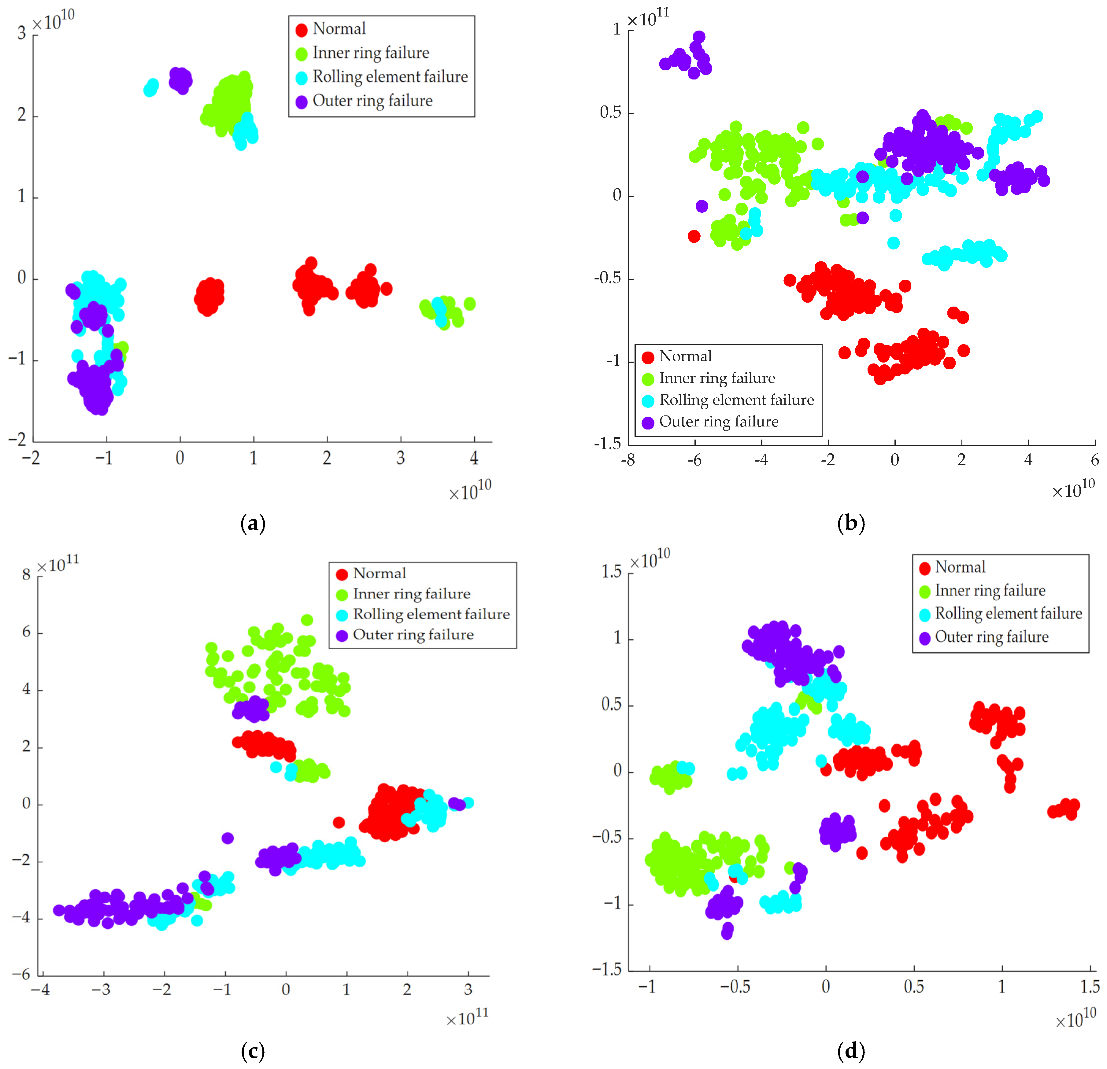
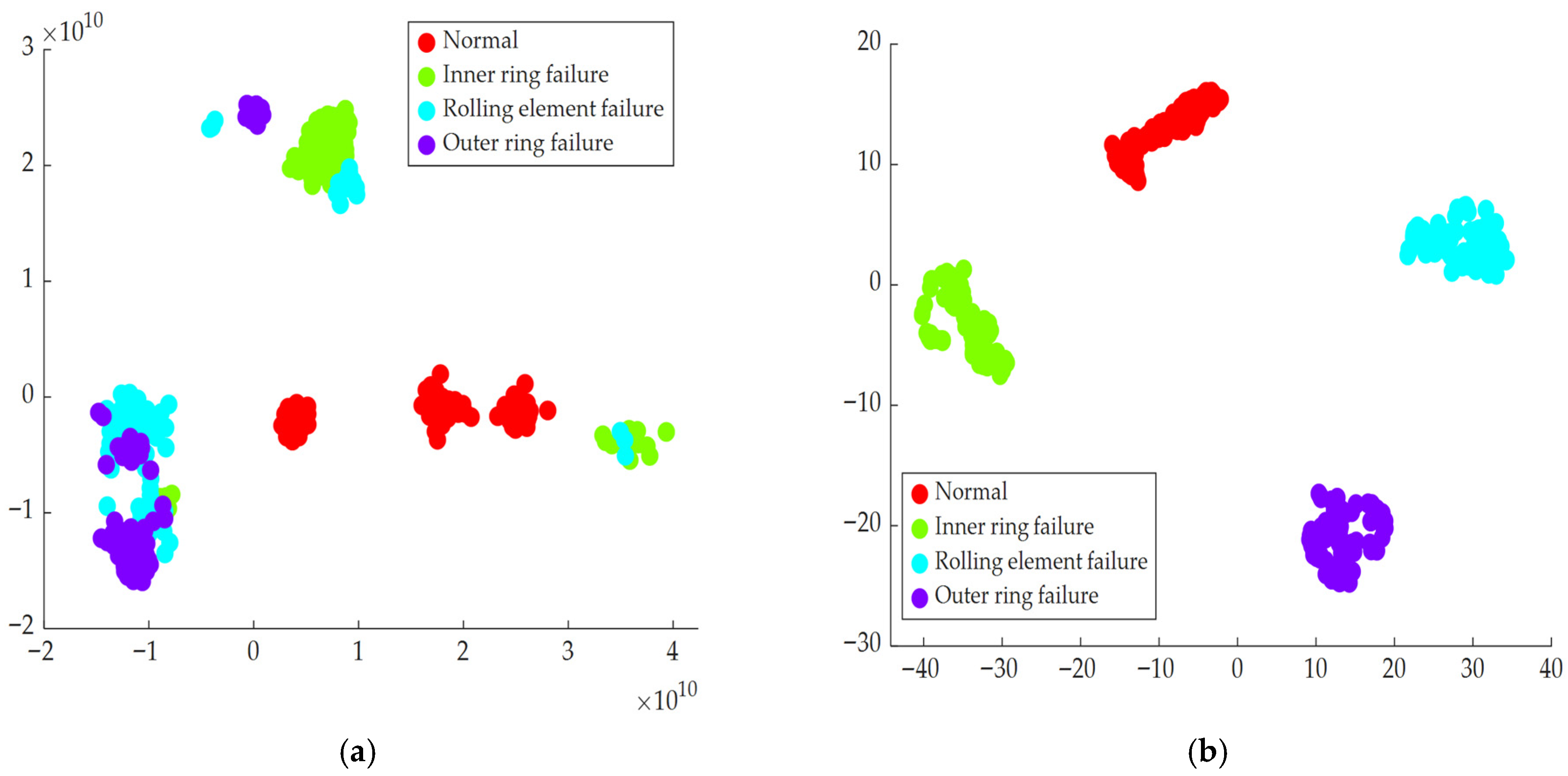
Subsequently, based on the aforementioned selection mechanism, time-domain reconstruction was performed on the target components, and the HFrAttE was further extracted. This algorithm deeply couples the nonlinear characterization capability of fractional-order entropy in processing non-stationary signals with the advantages of hierarchical decomposition in multi-band fine analysis. The objective is to construct a feature vector capable of comprehensively mapping the operating state of the bearing. To verify the discrimination efficacy of HFrAttE in the feature space, Multiscale Dispersion Entropy (MDE), Multiscale Approximate Entropy (MAE), and Multiscale Permutation Entropy (MPE) were introduced as control groups. Furthermore, the t-Distributed Stochastic Neighbor Embedding (t-SNE) algorithm was utilized to perform dimensionality reduction and visualization processing on the high-dimensional feature sets extracted from the noise-free data group.
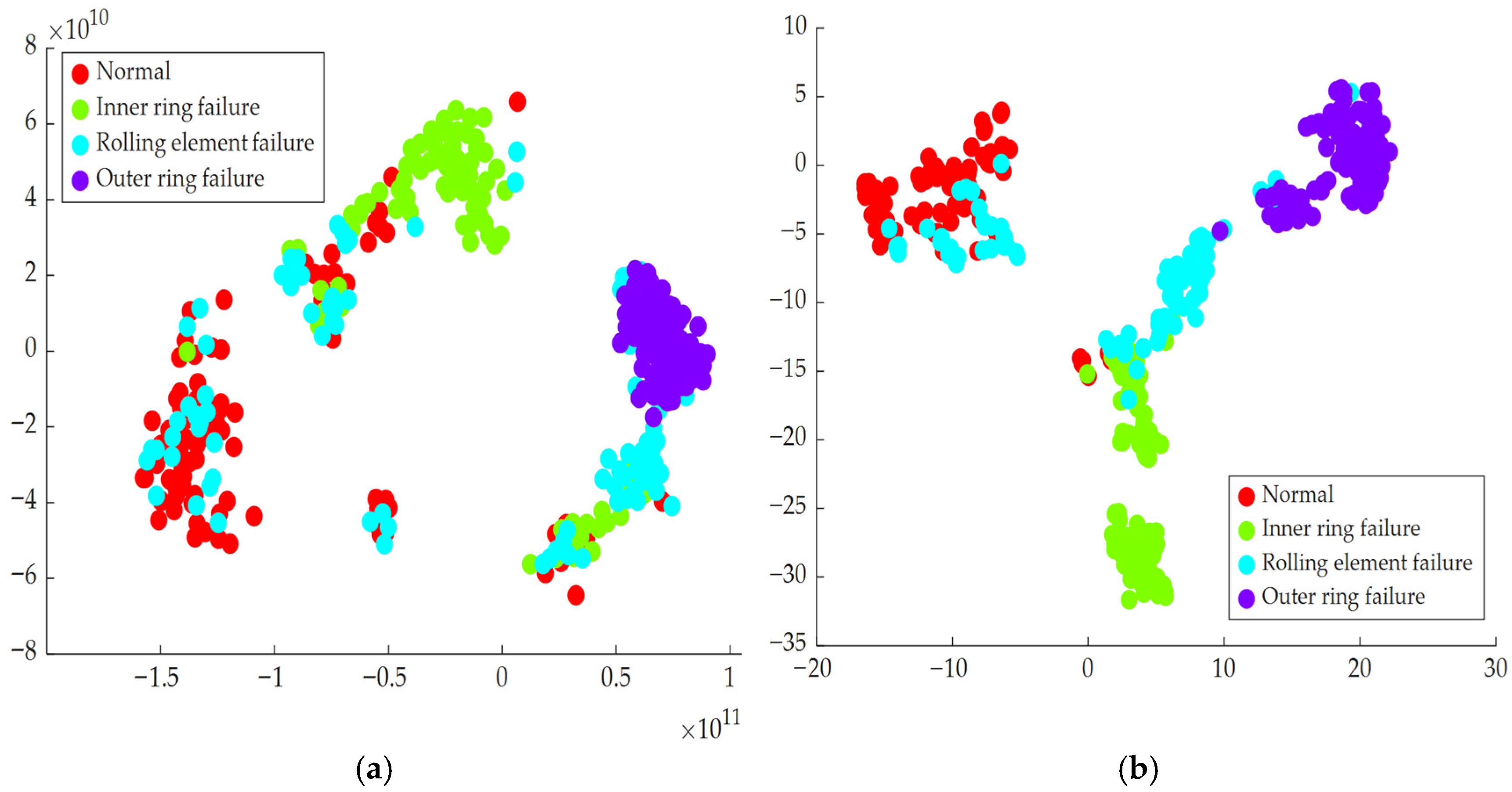
The two-dimensional projection results shown in Figure 23 indicate that, compared to the benchmark features, the feature space constructed by HFrAttE exhibits superior class separability. Under the four experimental conditions, the data points basically form independent clusters with clear boundaries on the manifold plane, demonstrating relatively strong intra-class consistency and inter-class separation. In contrast, for the three traditional multiscale features, their projected point sets exhibit varying degrees of cross-category overlap and spatial dispersion, making it difficult to achieve high-precision decoupling of complex operating states.
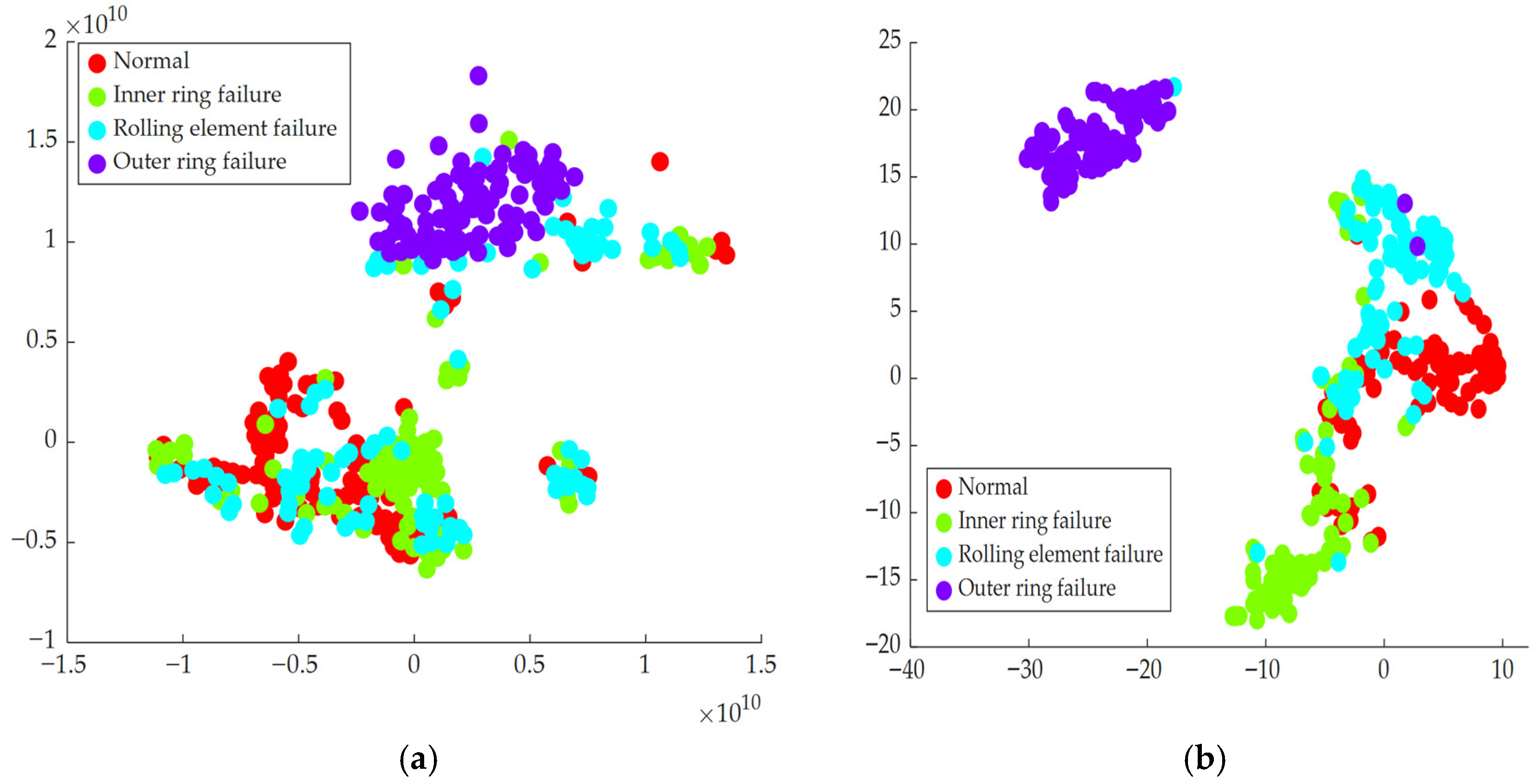
To deeply characterize the high-order discriminative information within HFrAttE, an Improved Transformer architecture was employed as the core feature refinement module. Subsequently, this module was coupled with the TELM classifier to jointly accomplish the decision mapping of the enhanced feature space. Based on the t-SNE visualization analysis presented in Figure 24, Figure 25 and Figure 26, it is observed that under noise-free conditions, the four bearing operating states achieved complete manifold separation. As the noise intensity gradient increased to −2 dB and even −5 dB, although the distribution of feature points exhibited a dispersion trend due to noise interference, leading to a certain degree of topological structure distortion, the deep features extracted by the improved architecture effectively retained key discriminative information. This provides reliable feature support for fault diagnosis under complex operating conditions.
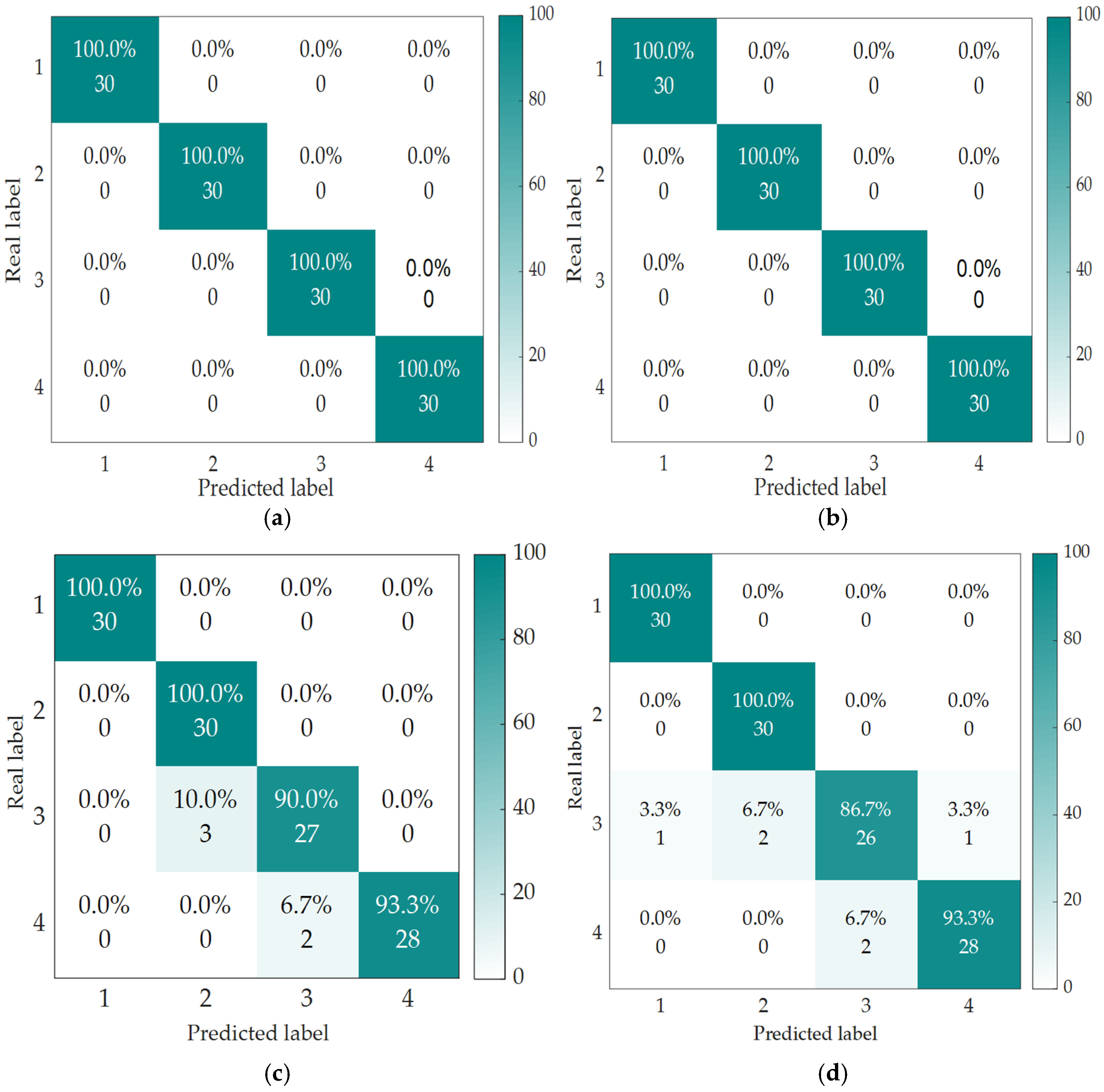
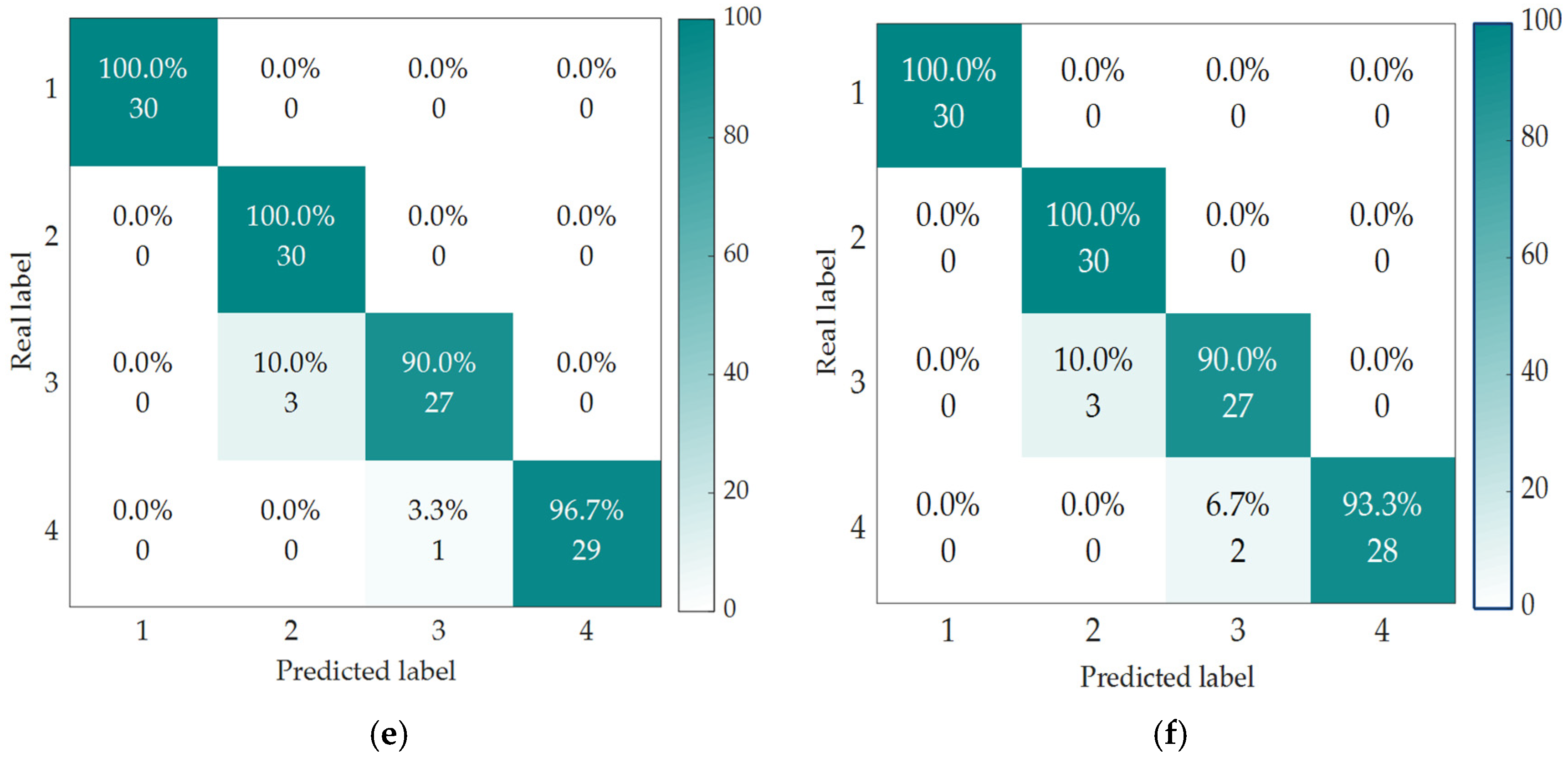
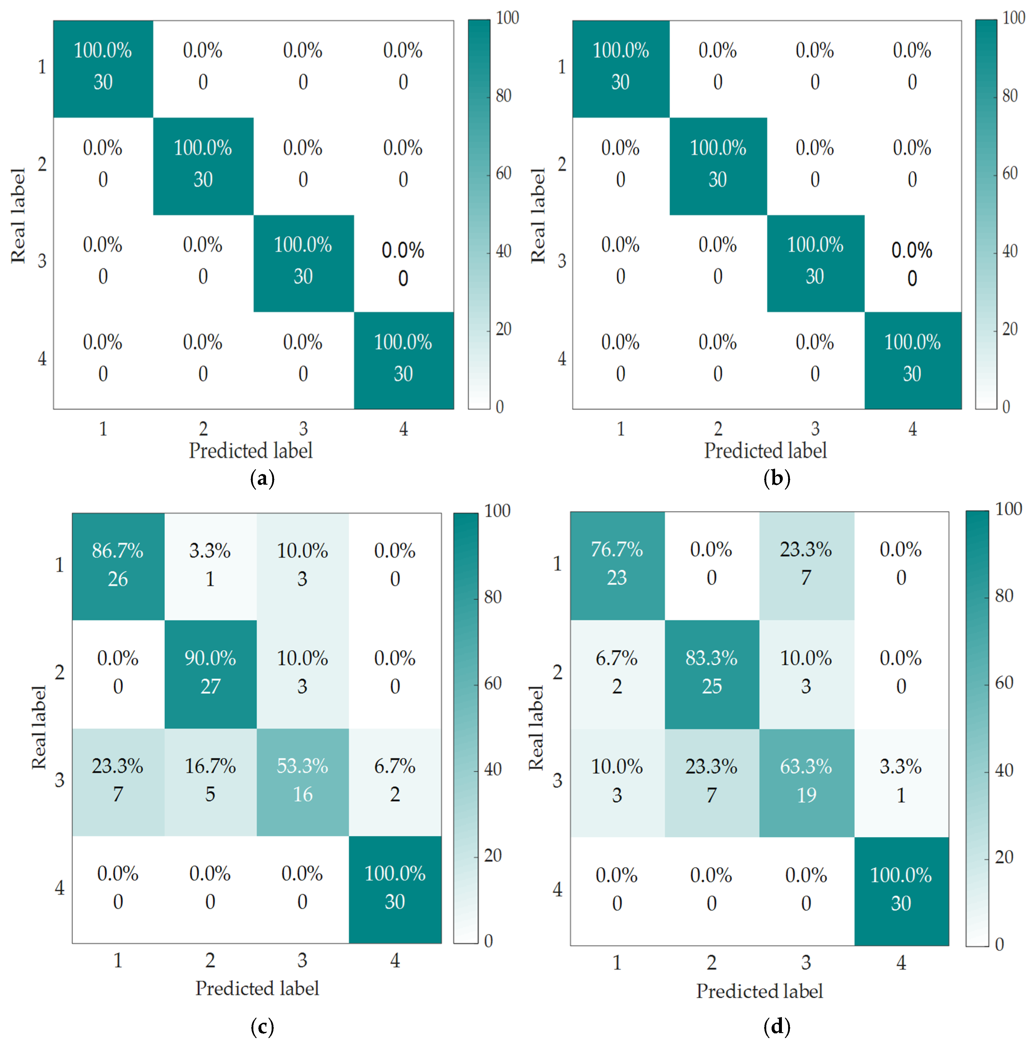
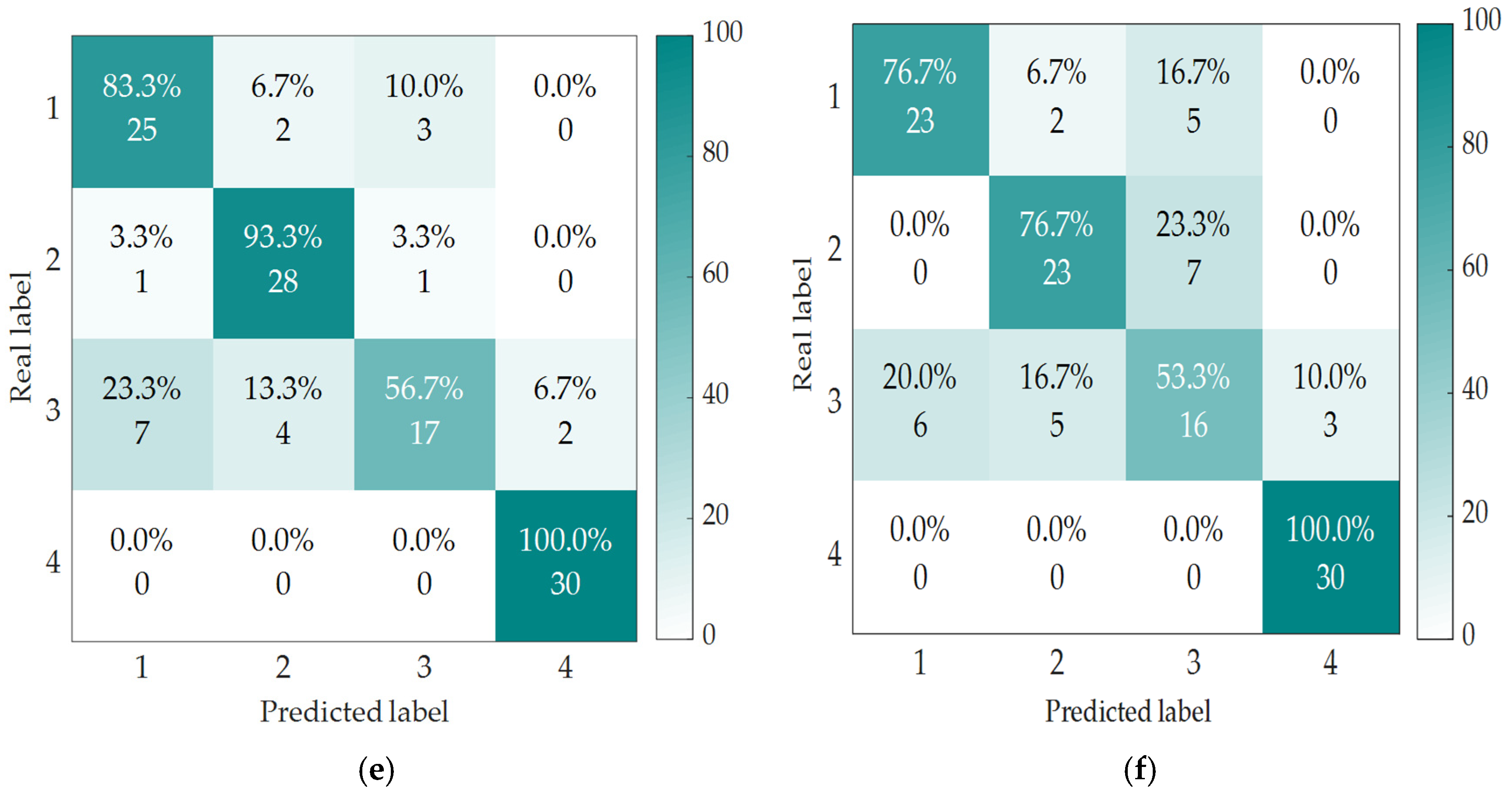
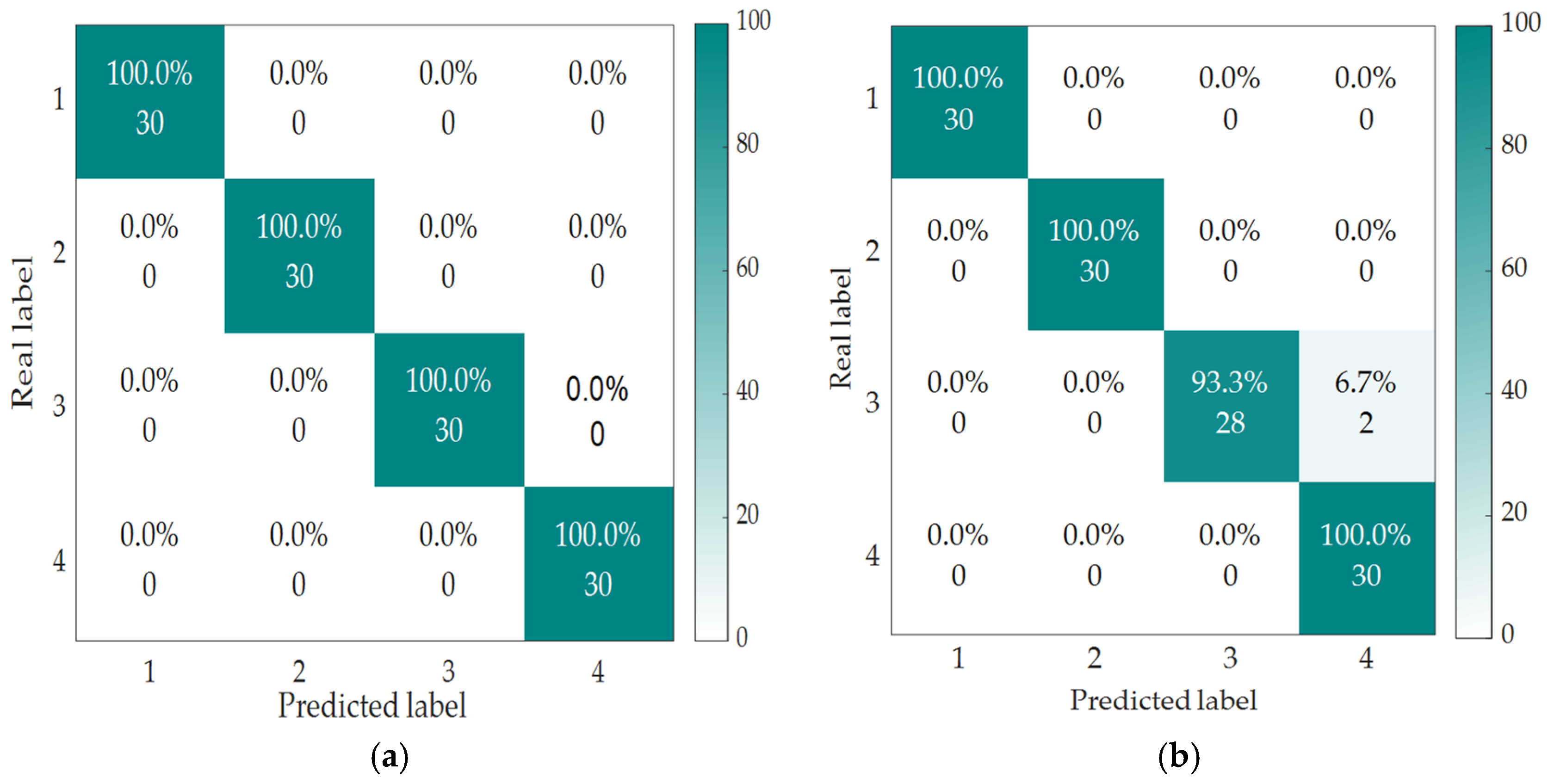
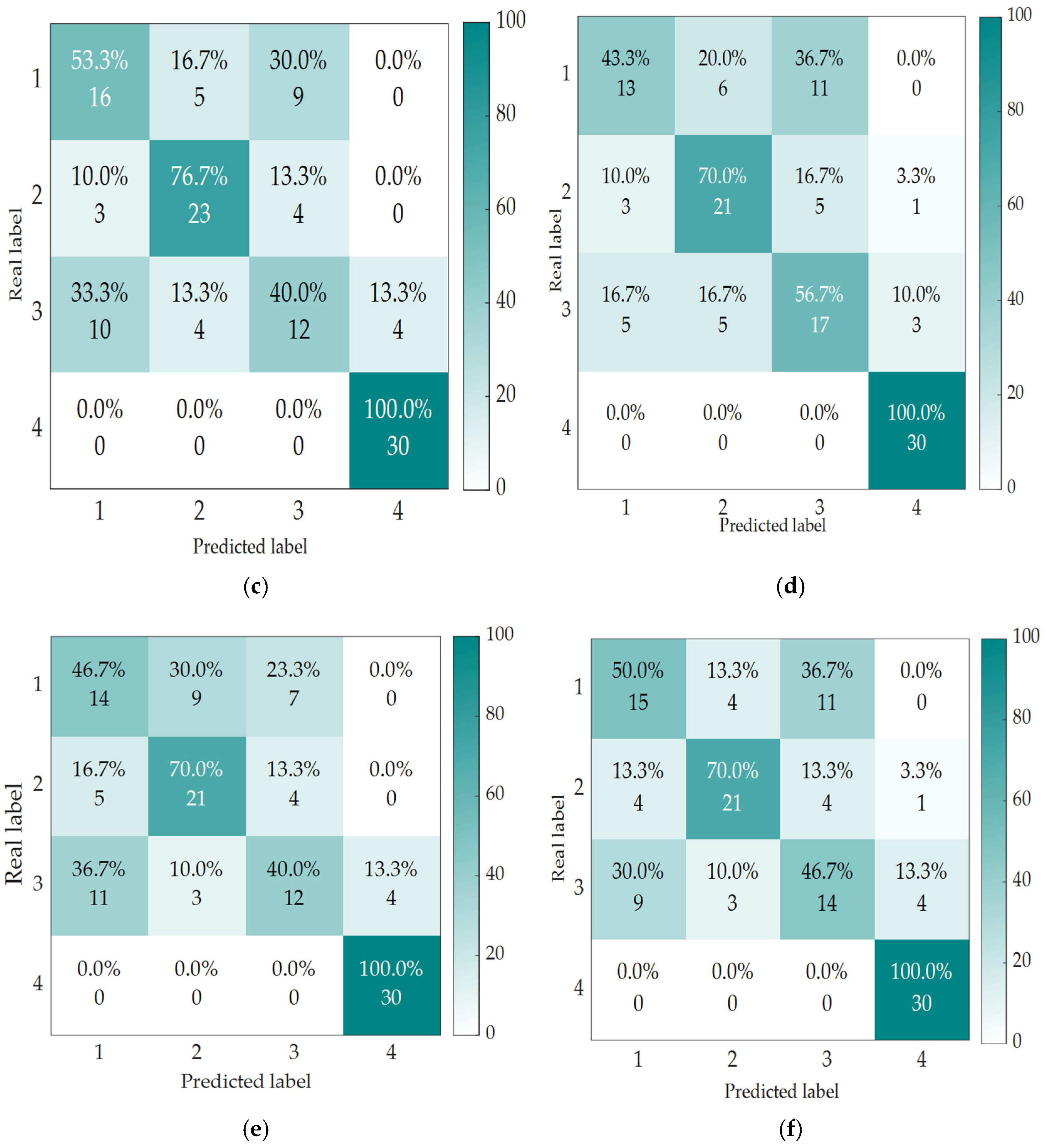
In the experimental evaluation phase, an end-to-end intelligent fault diagnosis framework was constructed by leveraging the highly discriminative deep features extracted via the Improved Transformer architecture. The TELM was integrated as the core classifier to achieve the identification of bearing operating states. To objectively evaluate the performance advantages of the proposed diagnostic scheme, benchmark models based on the same preprocessing workflow (i.e., optimized by IBKA-VMD)—including Transformer-TELM, Transformer-SVM, Transformer-KELM, Transformer-ELM, and Transformer-Softmax—were synchronously introduced as reference groups. This study specifically investigated the performance evolution patterns of the diagnostic models under differentiated signal-to-noise ratios (SNRs): a noise-free environment, −2 dB background noise, and −5 dB background noise. The classification decision logic and misdiagnosis distributions were visualized through refined modeling of multiple confusion matrices (see Figure 27, Figure 28 and Figure 29).
Regarding model evaluation, a comprehensive “trinity” quantification system was established, comprising Accuracy, Recall, and the F1-measure. The specific metric values obtained from the experiments are detailed in Table 3. Under ideal noise-free conditions, the proposed IBKA-VMD-Improved Transformer-TELM model, along with the comparative IBKA-VMD-Transformer-TELM architecture, achieved the theoretical peak of 100% across all three core metrics. In contrast, the traditional benchmark group exhibited slight recognition bottlenecks: the accuracy of Transformer-SVM, Transformer-KELM, Transformer-ELM, and Transformer-Softmax was recorded at 95.833%, 96.667%, 95.000%, and 95.833%, respectively. Their corresponding recall rates were 95.833%, 96.667%, 95.000%, and 95.833%, while the F1-scores were distributed at 95.829%, 96.662%, 94.926%, and 95.829%, respectively. These results preliminarily confirmed the positive significance of introducing the Improved Transformer in the feature extraction stage and the TELM classifier for enhancing complex fault clustering effects.
With the introduction of a −2 dB noise load, significant performance differentiation was observed among the robustness thresholds of the models. Experimental data indicated that the proposed Improved Transformer-TELM architecture, as well as the standard Transformer-TELM, maintained strong anti-interference capabilities, retaining a 100% recognition level across all evaluation metrics. However, the performance of the remaining four benchmark models exhibited a distinct attenuation trend: the recognition accuracy of Transformer-SVM, Transformer-KELM, Transformer-ELM, and Transformer-Softmax dropped to 82.50%, 83.333%, 80.833%, and 76.667%, respectively. Concurrent with the decline in accuracy, their recall and F1-scores also showed a synchronous contraction. This divergence suggests that traditional classifiers struggle to maintain stable decision boundaries when confronted with feature manifolds blurred by background noise, whereas the feature enhancement scheme adopted in this study effectively filters out environmental interference.
Under the more stringent −5 dB noise environment, the performance metrics of the benchmark models exhibited a degree of “systematic collapse.” In this working condition, the proposed IBKA-VMD-Improved Transformer-TELM architecture demonstrated superior representation robustness, with all evaluation metrics remaining firmly at 100%. Notably, the previously high-performing standard Transformer-TELM model began to exhibit performance fluctuations, with its precision, recall, and F1-score slightly declining to 98.333%, 98.333%, and 98.331%, respectively. In stark contrast, the diagnostic efficacy of the remaining benchmark models plummeted: the precision of Transformer-SVM, Transformer-KELM, Transformer-ELM, and Transformer-Softmax was only 67.5%, 64.167%, 67.5%, and 66.667%, respectively, with severe degradation observed in both recall and F1-scores. In summary, this significant performance comparison robustly demonstrates that the IBKA-VMD-Improved Transformer-TELM architecture possesses deeper feature mining potential and classification robustness under complex working conditions, providing reliable technical support for intelligent bearing operation and maintenance in complex industrial environments.

5. Conclusions

This study proposes an improved Transformer fault diagnosis method driven by the synergy of an IBKA-VMD and HFrAttE. Through the validation of the optimization performance of IBKA and experimental analysis of measured data from rolling bearings, the main conclusions are as follows:
(1)
To address the challenge of determining key parameters in VMD, this study enhances the IBKA by incorporating Tent chaotic mapping, golden sine guidance, and a dynamic hybrid mutation strategy. Experiments demonstrate that IBKA can adaptively identify the optimal number of decomposition layers and penalty factors for VMD, fundamentally suppressing modal aliasing and end effects inherent in traditional decomposition methods. Furthermore, the integration of a weighted index constructed from the square envelope spectrum kurtosis and square envelope spectrum Gini coefficient, along with a dynamic threshold screening strategy, enables precise reconstruction of sensitive components rich in fault impulses, effectively achieving signal purification amid strong background noise.
(2)
In terms of intrinsic feature representation, this study introduces HFrAttE. This metric addresses the limited sensitivity of traditional entropy metrics in describing the dynamic complexity of non-stationary vibration signals by leveraging the nonlinear gain effect of fractional-order operators on signal details, combined with a hierarchical multi-scale decomposition framework. Visual comparative analysis in the feature space confirms that the features extracted by this method exhibit relatively good intra-cluster cohesion and inter-cluster separability, providing a highly discriminative data foundation for subsequent feature mining by deep models.
(3)
At the fault identification decision-making level, an improved Transformer model that integrates a fully bidirectional attention mechanism and a high-dimensional feature decoupling structure is designed, and a TELM classifier is used to replace the traditional output layer. The bidirectional attention mechanism enables global capture of long-range dependencies in time-series signals, while the decoupling structure significantly enhances the robust representation capability of features. Comparative experimental analysis shows that under complex noise interference, this method significantly outperforms traditional models such as KELM, ELM, SVM, Softmax, and the standard Transformer in key evaluation metrics including accuracy, recall, and F1 score. In particular, in an environment with −5 dB noise added, the model still maintains 100% accuracy, providing an efficient and robust solution for intelligent operation and maintenance of rotating machinery.

6. Limitations and Future Work

Although the method proposed in this paper demonstrates favorable diagnostic performance in experiments, from the perspective of practical engineering applications, there are still certain limitations that require improvement:
(1)
Trade-off in computational cost: The multi-stage framework constructed in this paper, which integrates “multi-strategy optimization + adaptive decomposition + high-order feature extraction + deep learning,” significantly enhances recognition accuracy under complex operating conditions. However, it consumes more computational resources compared to single end-to-end models. When deployed in scenarios with extremely high real-time requirements or on embedded edge devices, further balancing algorithm complexity and processing efficiency may be necessary.
(2)
Generalization capability under complex operating conditions: This study has been thoroughly validated using the publicly available CWRU dataset. While this dataset is highly representative, actual industrial environments involve more complex variations in bearing types, operating speeds, and load conditions. The model’s generalizability when applied to entirely different types of rotating machinery or extreme non-stationary operating conditions still requires further empirical evaluation using more diverse datasets.
(3)
Sensitivity to empirical parameters: Some parameters within the framework are derived as empirical values based on the experimental environment in this study. Although these choices demonstrate robust performance across different signal-to-noise ratios, parameter sensitivity issues may arise in other mechanical systems with vastly different physical characteristics. Exploring more adaptive dynamic adjustment mechanisms is therefore essential.
Future research directions will focus on the following aspects: First, we plan to collect more naturally evolving fault data from real industrial sites and conduct empirical validation to enhance the model’s practical value. Second, we will explore model lightweighting techniques to facilitate integration of this framework into real-time online monitoring and edge computing platforms. Finally, we will investigate unsupervised or self-supervised learning-based pre-training mechanisms to reduce reliance on large-scale labeled data for intelligent diagnostics, thereby further improving system flexibility in actual operational and maintenance scenarios.

Author Contributions

Conceptualization, J.Y.; Methodology, J.Y., X.L. and M.M.; Software, J.Y., X.L. and M.M.; Validation, J.Y., X.L. and M.M.; Formal analysis, J.Y. and X.L.; Data curation, J.Y.; Writing—original draft, J.Y., X.L. and M.M.; Writing—review & editing, J.Y., X.L. and M.M.; Funding acquisition, J.Y. All authors have read and agreed to the published version of the manuscript.

Funding

This study was funded by the Yunnan Fundamental Research Projects (No. 202301AT070256), training Program for Baoshan Xingbao Talents (No. 202303), 10th batches of Baoshan young and middle-aged leaders training project in academic and technical (No. 202109), Zhejiang Provincial Natural Science Foundation of China under Grant (No. LQN26F030049), the Project of Quzhou Science and Technology Plan (No. 2025K232).

Data Availability Statement

The data presented in this study are available on request from the corresponding author upon request.

Conflicts of Interest

The authors declare no conflicts of interest.

References

  1. Durak, L.; Arikan, O. Short-time Fourier transform: Two fundamental properties and an optimal implementation. IEEE Trans. Signal Process. 2003, 51, 1231–1242. [Google Scholar] [CrossRef]
  2. Griffin, D.; Lim, J. Signal estimation from modified short-time Fourier transform. IEEE Trans. Acoust. Speech Signal Process. 1984, 32, 236–243. [Google Scholar] [CrossRef] [Scilit]
  3. Guo, T.; Zhang, T.; Lim, E.; Lopez-Benitez, M.; Ma, F.; Yu, L. A review of wavelet analysis and its applications: Challenges and opportunities. IEEE Access 2022, 10, 58869–58903. [Google Scholar] [CrossRef] [Scilit]
  4. Sun, G.; Wang, Y.; Luo, Q.; Li, Q. Vibration-based damage identification in composite plates using 3D-DIC and wavelet analysis. Mech. Syst. Signal Process. 2022, 173, 108890. [Google Scholar] [CrossRef] [Scilit]
  5. Ventricci, L.; Ribeiro Junior, R.F.; Gomes, G.F. Motor fault classification using hybrid short-time Fourier transform and wavelet transform with vibration signal and convolutional neural network. J. Braz. Soc. Mech. Sci. Eng. 2024, 46, 337. [Google Scholar] [CrossRef] [Scilit]
  6. Smith, J.S. The local mean decomposition and its application to EEG perception data. J. R. Soc. Interface 2005, 2, 443–454. [Google Scholar] [CrossRef] [Scilit]
  7. Huang, N.E.; Shen, Z.; Long, S.R.; Wu, M.C.; Shih, H.H.; Zheng, Q.; Yen, N.C.; Tung, C.C.; Liu, H.H. The empirical mode decomposition and the Hilbert spectrum for nonlinear and non-stationary time series analysis. Proc. R. Soc. London. Ser. A Math. Phys. Eng. Sci. 1998, 454, 903–995. [Google Scholar] [CrossRef] [Scilit]
  8. Yeh, J.R.; Shieh, J.S.; Huang, N.E. Complementary Ensemble Empirical Mode Decomposition: A novel noise enhanced data analysis method. Adv. Adapt. Data Anal. 2010, 2, 135–156. [Google Scholar] [CrossRef] [Scilit]
  9. Dhakar, A.; Singh, B.; Gupta, P. Diagnosing faults in rolling bearings of an air compressor set up using local mean decomposition and support vector machine algorithm. J. Vib. Eng. Technol. 2024, 12, 6635–6648. [Google Scholar] [CrossRef] [Scilit]
  10. Zhao, C.; Tong, B.; Zhou, C.; Fan, Q. Few-shot bearing fault diagnosis method based on an EEMD parallel neural network and a relation network. Adv. Mech. Eng. 2024, 16, 1–11. [Google Scholar] [CrossRef] [Scilit]
  11. Zhang, Y.; Zhang, Y.; Li, H.; Ming, W.; Du, W.; Wen, X.; Zhang, Y.; Yan, L. Semi-supervised diagnosis method for coupling faults of key rotating components based on EEMD-KPCA under cross working conditions. Meas. Sci. Technol. 2024, 35, 025014. [Google Scholar]
  12. Dragomiretskiy, K.; Zosso, D. Variational mode decomposition. IEEE Trans. Signal Process. 2013, 62, 531–544. [Google Scholar] [CrossRef] [Scilit]
  13. Wang, S.; Wang, C.; Lian, Y.; Luo, B. Research on Bearing Fault Diagnosis Based on VMD-RCMWPE Feature Extraction and WOA-SVM-Optimized Multidataset Fusion. Sensors 2025, 25, 5139. [Google Scholar] [CrossRef] [Scilit]
  14. Ma, Z.; Zhang, Y. A study on rolling bearing fault diagnosis using RIME-VMD. Sci. Rep. 2025, 15, 4712. [Google Scholar] [CrossRef] [Scilit]
  15. Li, Q.; Wu, C.; Lv, Q.; Wang, J. Application of GSABO-VMD-KELM in rolling bearing fault diagnosis. J. Vibroeng. 2025, 27, 1474–1497. [Google Scholar] [CrossRef] [Scilit]
  16. Dai, M.; Jo, H.; Kim, M.; Ban, S.W. MSFF-Net: Multi-sensor frequency-domain feature fusion network with lightweight 1D CNN for bearing fault diagnosis. Sensors 2025, 25, 4348. [Google Scholar] [CrossRef] [Scilit] [PubMed]
  17. Mohammad-Alikhani, A.; Jamshidpour, E.; Dhale, S.; Akrami, M.; Pardhan, S.; Nahid-Mobarakeh, B. Fault diagnosis of electric motors by a channel-wise regulated CNN and differential of STFT. IEEE Trans. Ind. Appl. 2025, 61, 3066–3077. [Google Scholar] [CrossRef] [Scilit]
  18. Shang, X.; Li, W.; Yuan, F.; Zhi, H.; Gao, Z.; Guo, M.; Xin, B. Research on Fault Diagnosis of UAV Rotor Motor Bearings Based on WPT-CEEMD-CNN-LSTM. Machines 2025, 13, 287. [Google Scholar] [CrossRef] [Scilit]
  19. Huang, Q.; Li, Z.; Fu, Z.; Hu, Y.; Fang, Q.; Wei, Y. Complex Wired Network Fault Diagnosis Based on Distributed Reflectometry and Multi-Channel 1D-CNN. IEEE Sens. J. 2025, 25, 19415–19427. [Google Scholar] [CrossRef] [Scilit]
  20. Liu, H.; Niu, B.; Liu, Z.; Li, M.; Shi, Z. Transformer fault diagnosis method based on the three-stage lightweight residual neural network. Electr. Power Syst. Res. 2025, 238, 111142. [Google Scholar] [CrossRef] [Scilit]
  21. Wu, M.; Zhang, J.; Xu, P.; Liang, Y.; Dai, Y.; Gao, T.; Bai, Y. Bearing fault diagnosis for cross-condition scenarios under data scarcity based on transformer transfer learning network. Electronics 2025, 14, 515. [Google Scholar] [CrossRef] [Scilit]
  22. Yang, Z.; Li, G.; Xue, G.; He, B.; Song, Y.; Li, X. A novel multi-sensor local and global feature fusion architecture based on multi-sensor sparse Transformer for intelligent fault diagnosis. Mech. Syst. Signal Process. 2025, 224, 112188. [Google Scholar] [CrossRef] [Scilit]
  23. Wan, Y.; Song, S.; Huang, G.; Li, S. Twin Extreme Learning Machines for Pattern Classification. Neurocomputing 2017, 260, 235–244. [Google Scholar] [CrossRef] [Scilit]
  24. Wang, J.; Wang, W.; Hu, X.X.; Qiu, L.; Zang, H.F. Black-winged kite algorithm: A nature-inspired meta-heuristic for solving benchmark functions and engineering problems. Artif. Intell. Rev. 2024, 57, 98. [Google Scholar] [CrossRef] [Scilit]
  25. Du, C.; Zhang, J.; Fang, J. An innovative complex-valued encoding black-winged kite algorithm for global optimization. Sci. Rep. 2025, 15, 932. [Google Scholar] [CrossRef] [Scilit]
  26. Sun, H.; Yang, S. Range-free localization algorithm based on modified distance and improved black-winged kite algorithm. Comput. Netw. 2025, 259, 111091. [Google Scholar] [CrossRef] [Scilit]
  27. Yang, J.-W.; Choudhary, G.I.; Rahardja, S.; Fränti, P. Classification of interbeat interval time-series using attention entropy. IEEE Trans. Affect. Comput. 2020, 14, 321–330. [Google Scholar] [CrossRef] [Scilit]
  28. Wang, W.J.; Gan, J. Bearing sub-health state identification based on optimal parameter VMD and improved dispersion entropy. J. Railw. Sci. Eng. 2025, 22, 887–899. [Google Scholar]
  29. Yuan, L.G.; Yang, X.T.; Yu, R.Z. Fractional-order approximate entropy. J. Xi’an Univ. Technol. 2020, 36, 575–580. [Google Scholar]
  30. Vaswani, A.; Shazeer, N.; Parmar, N.; Uszkoreit, J.; Jones, L.; Gomez, A.N.; Kaiser, Ł.; Polosukhin, I. Attention is All You Need. Adv. Neural Inf. Process. Syst. 2017, 30, 5998–6008. [Google Scholar]
  31. Yang, Y.; Han, C.; Ran, G.; Ma, T.; Pan, J. Fault Diagnosis of Rolling Element Bearing Based on BiTCN-Attention and OCSSA Mechanism. Actuators 2025, 14, 218. [Google Scholar] [CrossRef] [Scilit]
  32. Neupane, D.; Seok, J. Bearing fault detection and diagnosis using case western reserve university dataset with deep learning approaches: A review. IEEE Access 2020, 8, 93155–93178. [Google Scholar] [CrossRef] [Scilit]
  33. Raj, K.K.; Kumar, S.; Kumar, R.R.; Andriollo, M. Enhanced fault detection in bearings using machine learning and raw accelerometer data: A case study using the Case Western Reserve University dataset. Information 2024, 15, 259. [Google Scholar] [CrossRef] [Scilit]
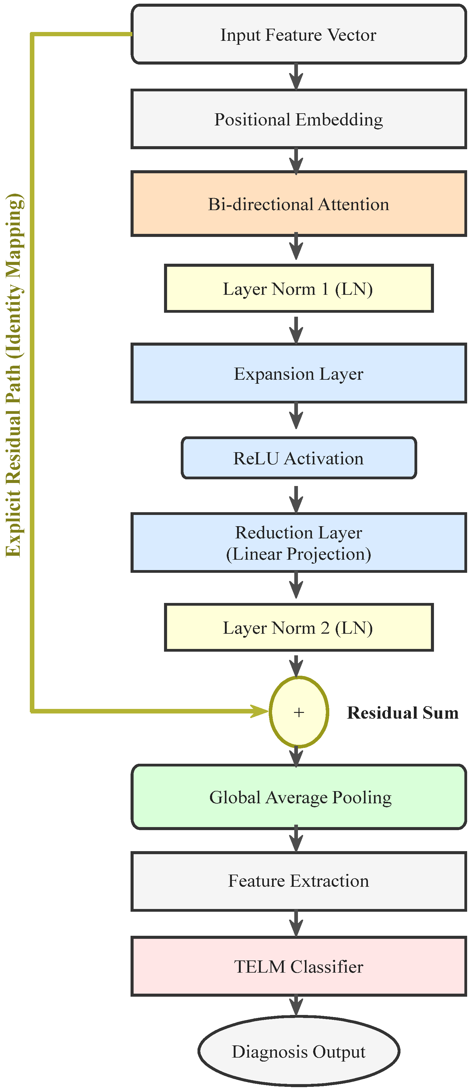
Figure 1. Structure of the improved Transformer model.
Fractalfract 10 00195 g001
Figure 2. Basic structure of ELM.
Fractalfract 10 00195 g002
Figure 3. Optimization process of IBKA.
Fractalfract 10 00195 g003
Figure 4. F3 function comparison results.
Fractalfract 10 00195 g004
Figure 5. F6 function comparison results.
Fractalfract 10 00195 g005
Figure 6. F9 function comparison results.
Fractalfract 10 00195 g006
Figure 7. F10 function comparison results.
Fractalfract 10 00195 g007
Figure 8. F20 function comparison results.
Fractalfract 10 00195 g008
Figure 9. F27 function comparison results.
Fractalfract 10 00195 g009
Figure 10. F28 function comparison results.
Fractalfract 10 00195 g010
Figure 11. Equipment for fault detection. (a) comprehensive bearing performance evaluation platform. (b) rolling bearing.
Fractalfract 10 00195 g011
Figure 12. Time-domain waveforms for bearing normal operation (a) and inner ring fault (b).
Fractalfract 10 00195 g012
Figure 13. Time—domain waveforms for bearing outer ring fault (a) and rolling element fault (b).
Fractalfract 10 00195 g013
Figure 14. Fitness curve changes for bearing in normal state (a), inner ring fault (b), rolling element fault (c), and outer ring fault (d).
Fractalfract 10 00195 g014
Figure 15. Waveform diagram (a) and spectrum diagram (b) of VMD under normal operation conditions.
Fractalfract 10 00195 g015
Figure 16. Waveform diagram (a) and spectrum diagram (b) of VMD under inner race fault conditions.
Fractalfract 10 00195 g016
Figure 17. Waveform diagram (a) and spectrum diagram (b) of VMD under rolling element fault conditions.
Fractalfract 10 00195 g017
Figure 18. Waveform diagram (a) and spectrum diagram (b) of VMD under outer ring fault conditions.
Fractalfract 10 00195 g018
Figure 19. Bar chart of the WFI evaluation index (normal operating condition).
Fractalfract 10 00195 g019
Figure 20. Bar chart of the WFI evaluation index (inner race fault condition).
Fractalfract 10 00195 g020
Figure 21. Bar chart of the WFI evaluation index (rolling element fault condition).
Fractalfract 10 00195 g021
Figure 22. Bar chart of the WFI evaluation index (outer ring fault condition).
Fractalfract 10 00195 g022
Figure 23. t-SNE visualization of different feature values: HFrAttE (a), MDE (b), MAE (c), and MPE (d).
Fractalfract 10 00195 g023
Figure 24. Visualization comparison of training data with HFrAttE under noise-free conditions: (a) original data, (b) after improved Transformer processing.
Fractalfract 10 00195 g024
Figure 25. Visualization comparison of training data with HFrAttE under −2 dB noise: (a) original data, (b) after improved Transformer processing.
Fractalfract 10 00195 g025
Figure 26. Visualization comparison of training data with HFrAttE under −5 dB noise: (a) original data, (b) after improved Transformer processing.
Fractalfract 10 00195 g026
Figure 27. Comparison of Identification Results of Different Models under Noise-Free Conditions: (a) IBKA-VMD-ITransformer-TELM, (b) IBKA-VMD-Transformer-TELM, (c) IBKA-VMD-Transformer-SVM, (d) IBKA-VMD-Transformer-ELM, (e) IBKA-VMD-Transformer-KELM, (f) IBKA-VMD-Transformer-Softmax.
Fractalfract 10 00195 g027aFractalfract 10 00195 g027b
Figure 28. Comparison of Identification Results of Different Models with −2 dB Noise Added: (a) IBKA-VMD-ITransformer-TELM, (b) IBKA-VMD-Transformer-TELM, (c) IBKA-VMD-Transformer-SVM, (d) IBKA-VMD-Transformer-ELM, (e) IBKA-VMD-Transformer-KELM, (f) IBKA-VMD-Transformer-Softmax.
Fractalfract 10 00195 g028aFractalfract 10 00195 g028b
Figure 29. Comparison of Identification Results of Different Models with −5 dB Noise Added: (a) IBKA-VMD-ITransformer-TELM, (b) IBKA-VMD-Transformer-TELM, (c) IBKA-VMD-Transformer-SVM, (d) IBKA-VMD-Transformer-ELM, (e) IBKA-VMD-Transformer-KELM, (f) IBKA-VMD-Transformer-Softmax.
Fractalfract 10 00195 g029aFractalfract 10 00195 g029b
Table 1. Performance benchmarking of selected CEC2017 experimental functions.
FunctionIndexIBKAGOOSEPSOGWOWOAGJOBKA
F3Std3.828 × 10−21.032 × 10−52.360 × 10−142.379 × 1031.097 × 1031.519 × 1031.838 × 101
Ave3.000 × 1023.000 × 1023.000 × 1021.689 × 1031.134 × 1031.792 × 1033.071 × 102
median3.000 × 1023.000 × 1023.000 × 1025.237 × 1026.309 × 1027.754 × 1023.006 × 102
F6Std9.940 × 10−11.244 × 1014.538 × 10−11.359 × 1001.280 × 1014.747 × 1009.640 × 100
Ave6.002 × 1026.519 × 1026.002 × 1026.013 × 1026.327 × 1026.053 × 1026.236 × 102
median6.000 × 1026.492 × 1026.000 × 1026.007 × 1026.341 × 1026.040 × 1026.249 × 102
F9Std2.705 × 1006.391 × 1028.640 × 10−22.104 × 1014.172 × 1026.873 × 1011.469 × 102
Ave9.006 × 1022.108 × 1039.000 × 1029.125 × 1021.466 × 1039.528 × 1021.192 × 103
median9.000 × 1021.966 × 1039.000 × 1029.008 × 1021.343 × 1039.444 × 1021.135 × 103
F10Std1.889 × 1022.863 × 1022.629 × 1023.329 × 1023.077 × 1023.556 × 1022.247 × 102
Ave1.447 × 1032.414 × 1031.564 × 1031.620 × 1032.117 × 1031.874 × 1031.799 × 103
median1.494 × 1032.396 × 1031.587 × 1031.538 × 1032.053 × 1031.868 × 1031.782 × 103
F20Std1.555 × 1011.433 × 1027.769 × 1016.135 × 1017.514 × 1014.549 × 1014.899 × 101
Ave2.024 × 1032.352 × 1032.079 × 1032.090 × 1032.152 × 1032.083 × 1032.083 × 103
median2.023 × 1032.356 × 1032.033 × 1032.058 × 1032.125 × 1032.060 × 1032.073 × 103
F25Std2.317 × 1012.487 × 1012.454 × 1012.100 × 1013.003 × 1012.822 × 1012.860 × 101
Ave2.915 × 1032.928 × 1032.929 × 1032.941 × 1032.942 × 1032.939 × 1032.925 × 103
median2.900 × 1032.946 × 1032.944 × 1032.945 × 1032.951 × 1032.944 × 1032.915 × 103
F27Std8.683 × 1009.102 × 1013.292 × 1011.405 × 1014.405 × 1011.275 × 1012.049 × 101
Ave3.093 × 1033.224 × 1033.126 × 1033.102 × 1033.142 × 1033.099 × 1033.104 × 103
median3.091 × 1033.204 × 1033.108 × 1033.095 × 1033.125 × 1033.095 × 1033.099 × 103
F28Std1.005 × 1021.644 × 1021.131 × 1021.039 × 1021.646 × 1021.195 × 1021.619 × 102
Ave3.238 × 1033.282 × 1033.302 × 1033.378 × 1033.357 × 1033.330 × 1033.279 × 103
median3.197 × 1033.384 × 1033.384 × 1033.401 × 1033.407 × 1033.246 × 1033.301 × 103
Table 2. IBKA optimized VMD result parameters.
Fault CategoryWithout Adding Noise−2 dB−5 dB
normala = 2303, k = 9a = 2012, k = 6a = 1300, k = 9
inner racea = 2840, k = 3a = 2269, k = 7a = 2847, k = 8
rolling elementa = 3000, k = 8a = 2353, k = 7a = 2542, k = 7
outer ringa = 100, k = 4a = 1128, k = 5a = 356, k = 7
Table 3. Comparison of Identification Results of Fault Diagnosis Models.
Noise SituationEvaluating IndicatorIBKA-VMD-Improved Transformer-TELMIBKA-VMD Transformer-TELMIBKA-VMD Transformer- SVMIBKA-VMD-Transformer-KELMIBKA-VMD-Transformer-ELMIBKA-VMD-Transformer-Softmax
Without noise additionAccuracy/%10010095.83396.6679595.833
Recall/%10010095.83396.6679595.833
F1 measure/%10010095.82996.66294.92695.829
−2 dBAccuracy/%10010082.5083.33380.83376.667
Recall/%10010082.5083.33380.83376.667
F1 measure/%10010081.64282.57680.68176.261
−5 dBAccuracy/%10098.33367.564.16767.566.667
Recall/%10098.33367.564.16767.566.667
F1 measure/%10098.33166.45463.09266.61065.976
Disclaimer/Publisher’s Note: The statements, opinions and data contained in all publications are solely those of the individual author(s) and contributor(s) and not of MDPI and/or the editor(s). MDPI and/or the editor(s) disclaim responsibility for any injury to people or property resulting from any ideas, methods, instructions or products referred to in the content.