Analytical Pricing of Volatility-Linked Financial Derivatives Under the Sub-Mixed Fractional Brownian Motion Framework in a No-Arbitrage Complete Market

Abstract

This paper develops a unified analytical approach for pricing a broad class of volatility-linked financial derivatives under the sub-mixed fractional geometric Brownian motion model. The proposed framework captures key empirical features of financial markets, including correlated non-stationary Gaussian increments and long-memory dependence, while preserving the semimartingale property required for arbitrage-free pricing. We present the exact distribution of the realized variance as a quadratic form of correlated non-stationary Gaussian increments, which leads to a closed-form expression for the cumulative distribution function via a Laguerre-series expansion. These distributional results enable analytical pricing formulas for an extensive family of volatility-linked derivatives. Monte Carlo simulations confirm the accuracy and computational efficiency of the proposed formulas, while numerical investigations illustrate the significant impact of non-stationarity, long-memory effects, and the Hurst parameter on derivative values. These results contribute to a deeper theoretical understanding and more effective computational methods for pricing nonlinear volatility derivatives in markets characterized by persistent temporal dependence and non-stationary stochastic dynamics.

1. Introduction

Volatility-linked financial derivatives have emerged as a prominent class of financial instruments, capturing the interest of both researchers and market participants. Their relevance has been amplified by the increasing demand for tools that offer direct exposure to volatility, distinct from the directional movement of asset prices. This trend is well documented in a growing body of literature and is reflected in the evolving practices of modern financial markets (see, e.g., [1,2,3,4,5]). Volatility, commonly quantified through the standard deviation of asset returns, is central to measuring uncertainty and serves as a critical input in option pricing models, portfolio risk control, and financial regulation.

As a consequence, instruments such as volatility swaps, variance swaps, and options on volatility have gained widespread use in financial practice. These products allow investors to take targeted positions on market volatility, independent of the direction or magnitude of underlying price changes. They also provide essential tools for hedging against volatility risk, managing portfolio sensitivity to market turbulence, and constructing arbitrage strategies that exploit discrepancies between implied and realized volatility. The ability to trade volatility directly has therefore expanded the scope of risk management and offered new opportunities for return generation.

Within this class of products, contracts linked to discretely observed log-return realized variance have attracted considerable interest. Prominent representatives include variance swaps and volatility swaps, both of which determine their terminal payoffs from the accumulated variance measured over a finite collection of observation dates. Despite this similarity, the two instruments differ substantially from an analytical perspective. The payoff of a variance swap depends linearly on the realized variance and therefore admits more tractable closed-form treatments. In contrast, volatility swaps involve a nonlinear transformation through the square root of the realized variance, which leads to pronounced analytical difficulties. These challenges are further exacerbated in discrete-time settings where the joint distribution of log-returns is not available in closed form, rendering the evaluation of expected payoffs particularly demanding.

The presence of temporal dependence and non-stationarity in log-returns further undermines analytical tractability. The square-root structure of aggregated correlated squared returns obstructs standard valuation approaches, leading volatility swap pricing to depend primarily on numerical integration or Monte Carlo (MC) simulation. While accurate, such methods are computationally demanding and less practical for real-time applications, motivating the development of efficient analytical and semi-analytical alternatives.

An important contribution to this line of research was provided by Rujivan and Rakwongwan [6], and later by Rujivan [7], who developed an analytical framework for volatility swap pricing within the classical Black–Scholes model with time-varying parameters. Their approach applies a Laguerre series expansion to the probability density function of discretely sampled log-return realized variance, yielding closed-form pricing formulas for a broad class of volatility-linked financial derivatives. This framework was subsequently extended to the Merton jump-diffusion model with a non-homogeneous Poisson jump process [8], thereby enlarging its range of applicability. A central feature of the methodology is the representation of discretely sampled realized variance as a conic combination of independent noncentral chi-square random variables, leveraging the independence of Brownian motion increments. This structure enables the use of classical expansion techniques, such as those developed in [9,10], resulting in an analytically tractable and computationally efficient pricing framework.

Existing approaches nonetheless rely on the assumption that asset prices evolve according to a geometric Brownian motion (GBm) with independent and stationary increments. In contrast, a substantial body of empirical evidence has documented the presence of long-range dependence and self-similarity in financial asset returns [11,12], features that are not captured by the classical Black–Scholes model. To accommodate such effects, Necula [13] introduced an extension of the Black–Scholes framework based on fractional Brownian motion (fBm), originally proposed by Kolmogorov [14]. The fBm framework incorporates long-memory dependence and has been extensively studied in financial modeling (see, e.g., [15,16,17]). However, except in the special case where the Hurst parameter satisfies $H=\frac{1}{2}$, fBm is neither a Markov process nor a semimartingale, which leads to arbitrage opportunities under classical trading strategies.

Although certain works (e.g., [18,19]) have attempted to accommodate the non-semimartingale nature of fractional processes through Wick-type self-financing strategies, such formulations have been criticized for their limited economic interpretability, as argued by Björk and Hult [20]. In response to these limitations, a growing body of literature has proposed alternative stochastic models that more accurately capture the empirical characteristics observed in financial markets. Notable among these are models incorporating fractional and mixed fractional Brownian motions, as investigated in [15,21,22,23,24]. These models are particularly well-suited for representing financial time series with non-stationary behavior—where the underlying statistical properties evolve over time—thereby offering a more realistic foundation for financial modeling.

Within the broader class of models aimed at capturing long-memory and evolving market dynamics, Bojdecki et al. [21] introduced the sub-fractional Brownian motion (sfBm)—a centered Gaussian process exhibiting both long-range dependence and non-stationary increments. These statistical characteristics make sfBm a compelling candidate for modeling financial time series, particularly in contexts where volatility clustering and persistent memory are empirically observed (see, e.g., [16,25,26]). However, like the fBm, sfBm does not possess the semimartingale property. This limitation imposes a significant barrier to its use in arbitrage-free pricing and dynamic hedging within complete market frameworks, as such models typically require semimartingale dynamics to support a risk-neutral valuation approach.

Within the family of stochastic models developed to capture persistent dependence and evolving market behavior, sub-fractional Brownian motion (sfBm), introduced in [21], is defined as a centered Gaussian process with long-range dependence and non-stationary increments. Such properties are consistent with empirical features commonly observed in financial time series, including volatility clustering and long-memory effects (see, e.g., [16,25,26]). Despite these advantages, sfBm suffers from the same structural limitation as fractional Brownian motion, namely the absence of the semimartingale property. This deficiency prevents sfBm-driven asset price models from being directly incorporated into arbitrage-free pricing and dynamic hedging frameworks in complete markets, where a semimartingale structure is required to define an equivalent risk-neutral measure.

To overcome these limitations, several authors have proposed the mixed fractional Brownian motion (mfBm), which superposes a standard Brownian motion component with a fractional Brownian motion component [27,28]. This hybrid construction preserves the long-memory features associated with fBm while recovering the semimartingale property under suitable parameter regimes. In particular, Cheridito [29] established that when the Hurst parameter satisfies $H\in \left(\frac{3}{4},1\right)$, mfBm is equivalent in distribution to standard Brownian motion, thereby allowing for arbitrage-free pricing within a complete market framework. Despite this advantage, mfBm inherits stationary increments, which restricts its capacity to capture the non-stationary dynamics frequently observed in empirical financial data.

To address this shortcoming, the sub-mixed fractional Brownian motion (smfBm) was introduced in [30] as a hybrid process formed by combining standard Brownian motion with sub-fractional Brownian motion. This construction preserves key empirical features observed in financial time series, including long-range dependence and non-stationary increments, while admitting a semimartingale representation for Hurst parameters $H\in \left(\frac{3}{4},1\right)$. Consequently, smfBm is compatible with arbitrage-free pricing in complete market frameworks, effectively reconciling statistical realism with mathematical tractability.

More recent contributions have demonstrated the flexibility of the sub-mixed fractional Brownian motion in capturing a broad spectrum of financial market behaviors, supporting its relevance for practical modeling purposes (see, e.g., [31,32]). On this basis, a growing body of work has developed analytical techniques for valuing both standard and exotic derivatives within the smfBm framework (see, for instance, [32,33,34,35,36]). Despite these advances, a unified and tractable analytical framework for pricing volatility-linked derivatives with nonlinear payoffs—such as volatility swaps and volatility options—remains largely absent in the existing literature under the smfBm setting. The present work fills this gap by introducing a rigorous valuation methodology within the sub-mixed fractional geometric Brownian motion (smfGBm) framework, thereby extending the analytical toolkit for volatility derivative pricing in markets characterized by long-memory dependence and non-stationary dynamics.

A central analytical difficulty in the valuation of volatility-linked derivatives under the smfBm framework arises from the fact that, whenever $H\ne \frac{1}{2}$, the increments of smfBm exhibit both correlation and non-stationarity, as documented in [30]. These characteristics invalidate a wide range of classical analytical tools that depend on independent or stationary increment assumptions (see, e.g., [6,7,8,9,10]), thereby necessitating a fundamentally different methodological approach. In the present work, we build on a recent analytical strategy developed in [37] for volatility derivative pricing under the mfBm setting, where the discretely sampled log-return realized variance is shown to admit an exact representation as a quadratic form of correlated, non-stationary Gaussian increments. This representation allows for an explicit characterization of the cumulative distribution function of the realized variance through a Laguerre series expansion. The resulting distributional formulation faithfully reflects the intricate dependence patterns generated by long-memory effects and non-stationary dynamics, and serves as the analytical backbone of the valuation framework proposed in this study.

Exploiting the explicit closed-form expression of the realized variance distribution, we derive analytical pricing formulas for a wide range of volatility-linked derivatives with nonlinear payoffs. These include variance and volatility options, capped and floored variance and volatility swaps, knock-out variance and volatility contracts, as well as knocking-out corridor variance and volatility products. The resulting expressions are fully explicit and computationally efficient, providing practical alternatives to standard numerical procedures that become prohibitively costly in the presence of correlated, non-stationary Gaussian increments. The validity and numerical performance of the proposed pricing framework are examined through MC simulations, which demonstrate excellent consistency with the analytical formulas. In addition, the numerical results highlight a strong dependence of fair strike values on the Hurst parameter H, emphasizing the necessity of accounting for long-memory effects and non-stationary dynamics in the valuation of volatility-related financial instruments.

It is worth stressing that, although the present work is closely related to our earlier study conducted under the mfGBm framework [37], the contributions of the two approaches differ both conceptually and technically. Unlike the mfGBm model, in which the driving noise possesses stationary increments, the smfBm setting considered here generates discretely sampled log-returns with correlated and non-stationary Gaussian increments. This intrinsic structural distinction gives rise to a substantially different covariance structure for realized variance and calls for new analytical tools. Specifically, while the mfGBm framework admits a Laguerre-series representation for the probability density function of discretely sampled realized variance, the smfBm-based methodology developed in this paper yields explicit Laguerre-series representations for both the probability density function and the cumulative distribution function. The availability of a closed-form CDF is a key methodological enhancement, as it facilitates a unified and numerically stable pricing approach in which valuation formulas for a broad class of nonlinear volatility-linked derivatives are expressed directly in terms of the distribution function, rather than relying on density-based or moment-based characterizations. This CDF-driven formulation significantly improves numerical robustness, particularly for payoffs that are sensitive to tail behavior, such as option contracts, capped or floored instruments, and knock-out or corridor-type structures, and thus represents a substantive extension beyond the mfGBm-based framework.

This paper is organized as follows. Section 2 reviews the fundamental distributional properties of smfBm increments that underpin the proposed methodology and introduces the smfGBm model adopted for asset price dynamics. In Section 3, we establish explicit Laguerre-series representations for both the probability density function and the cumulative distribution function of the discretely sampled log-return realized variance, together with a careful examination of truncation errors. This section also develops analytical valuation formulas for the class of volatility-linked derivatives considered in the study. Section 4 reports MC simulation results that corroborate the accuracy and computational performance of the proposed pricing approach and examines the sensitivity of fair strike prices with respect to variations in the Hurst parameter. Concluding remarks are provided in Section 5, where the main results are summarized and their theoretical and practical implications are discussed. Detailed mathematical proofs are deferred to the Appendix A and Appendix B.

2. Sub-Mixed Fractional Geometric Brownian Motion Model

2.1. Fractional and Sub-Fractional Brownian Motions

Let $(\mathrm{\Omega },\mathcal{F},\mathbb{P})$ be a probability space. A stochastic process ${\left(B_t^{\left(H\right)}\right)}_{t\in \mathbb{R}}$ is called a fractional Brownian motion (fBm) on the real line with Hurst parameter $H\in (0,1)$ if it is a centered Gaussian process that is almost surely continuous under $\mathbb{P}$, satisfies $B_0^{\left(H\right)}=0$ almost surely, and has stationary increments. The covariance function of fBm is given by

$$\mathrm{Cov}\left(B_t^{\left(H\right)},B_s^{\left(H\right)}\right)={\displaystyle \frac{1}{2}}\left({\left|t\right|}^{2H}+{\left|s\right|}^{2H}-{|t-s|}^{2H}\right),\forall s,t\in \mathbb{R}.$$

(1)

Consequently, the variance of the increment over the interval $[s,t]$ is

$$\mathrm{Var}\left(B_t^{\left(H\right)}-B_s^{\left(H\right)}\right)={|t-s|}^{2H},$$

(2)

for all $s,t\in (0,\infty )$ with $s\ne t$. This property confirms that fractional Brownian motion has stationary increments, in the sense that the distributional characteristics of $B_t^{\left(H\right)}-B_s^{\left(H\right)}$ depend solely on the time difference $|t-s|$ and not on the specific values of t and s.

For $H={\displaystyle \frac{1}{2}}$, the process ${\left(B_t^{(1/2)}\right)}_{t\in \mathbb{R}}$ coincides with the standard Bm on the real line, denoted by ${\left(B_t\right)}_{t\in \mathbb{R}}$.

We introduce the sub-fractional Brownian motion (sfBm), defined as:

$${\xi }_t^{\left(H\right)}:={\displaystyle \frac{B_t^{\left(H\right)}+B_{-t}^{\left(H\right)}}{\sqrt{2}}},t\in {\mathbb{R}}^{+}.$$

(3)

The process ${\left({\xi }_t^{\left(H\right)}\right)}_{t\ge 0}$ is defined on $(\mathrm{\Omega },\mathcal{F},\mathbb{P})$ with respect to the filtration ${\left({\mathcal{F}}_t^{{\xi }^{\left(H\right)}}\right)}_{t\ge 0}$ generated by ${\left({\xi }_t^{\left(H\right)}\right)}_{t\ge 0}$, which satisfies the usual conditions.

The key properties of the process ${\left({\xi }_t^{\left(H\right)}\right)}_{t\ge 0}$, as introduced by [30], are summarized as follows:

Proposition 1.

Let $H\in (0,1)$. The sfBm ${\left({\xi }_t^{\left(H\right)}\right)}_{t\ge 0}$, defined by (3), satisfies the following properties:

1. 

${\left({\xi }_t^{\left(H\right)}\right)}_{t\ge 0}$ is a $\mathbb{P}$-almost surely continuous, centered Gaussian process with ${\xi }_0^{\left(H\right)}=0$, almost surely.

2. 

${\left({\xi }_t^{\left(H\right)}\right)}_{t\ge 0}$ does not have stationary increments when $H\ne \frac{1}{2}$. In addition, for $s,t\in {\mathbb{R}}^{+}$ and $s\ne t$, the variance of its increment is:

$$\mathit{Var}\left({\xi }_t^{\left(H\right)}-{\xi }_s^{\left(H\right)}\right)=-2^{2H-1}\left(t^{2H}+s^{2H}\right)+{(t+s)}^{2H}+{|t-s|}^{2H}.$$

3. 

The covariance function of ${\xi }_t^{\left(H\right)}$ is:

$$\mathit{Cov}\left({\xi }_t^{\left(H\right)},{\xi }_s^{\left(H\right)}\right)=t^{2H}+s^{2H}-{\displaystyle \frac{1}{2}}\left({(t+s)}^{2H}+{|t-s|}^{2H}\right)\ge 0,\forall s,t\in {\mathbb{R}}^{+}.$$

4. 

The variance of ${\xi }_t^{\left(H\right)}$ is:

$$\mathit{Var}\left({\xi }_t^{\left(H\right)}\right)=\left(2-2^{2H-1}\right)t^{2H},\forall t\in {\mathbb{R}}^{+}.$$

5. 

The covariance satisfies:

$$0<\mathit{Cov}\left({\xi }_t^{\left(H\right)},{\xi }_s^{\left(H\right)}\right)<\mathit{Cov}\left(B_t^{\left(H\right)},B_s^{\left(H\right)}\right)\mathit{if}H\in \left(\frac{1}{2},1\right),\forall s,t\in {\mathbb{R}}^{+}.$$

2.2. Sub-Mixed Fractional Brownian Motions

A stochastic process known as the sub-mixed fractional Brownian motion (smfBm), originally proposed in [30], is constructed as a superposition of a standard Brownian motion and a sub-fractional Brownian motion. Specifically, it is defined by

$${\widehat{M}}_t^{\left(H\right)}\equiv {\widehat{M}}_t^{\left(H\right)}({\widehat{\sigma }}_B,{\widehat{\sigma }}_F)={\widehat{\sigma }}_B{B}_t+{\widehat{\sigma }}_F{\xi }_t^{\left(H\right)},t\in {\mathbb{R}}^{+},$$

(4)

where ${\left(B_t\right)}_{t\ge 0}$ denotes a standard Brownian motion. The constants ${\widehat{\sigma }}_B>0$ and ${\widehat{\sigma }}_F\ge 0$ act as intensity parameters, governing the relative contributions of the Brownian and sub-fractional Brownian components, respectively.

Throughout this work, the processes ${\left(B_t\right)}_{t\ge 0}$ and ${\left({\xi }_t^{\left(H\right)}\right)}_{t\ge 0}$ are assumed to be independent. The smfBm ${\left({\widehat{M}}_t^{\left(H\right)}\right)}_{t\ge 0}$ is defined on a probability space $(\mathrm{\Omega },\mathcal{F},\mathbb{P})$ and is adapted to the filtration ${\left({\mathcal{F}}_t^{{\widehat{M}}^{\left(H\right)}}\right)}_{t\ge 0}$ generated by the process itself. This filtration is assumed to satisfy the usual hypotheses of completeness and right-continuity.

The main structural characteristics of the smfBm process ${\left({\widehat{M}}_t^{\left(H\right)}\right)}_{t\ge 0}$, established in [30], are summarized in the following proposition.

Proposition 2.

Let $H\in (0,1)$. The process ${\left({\widehat{M}}_t^{\left(H\right)}\right)}_{t\ge 0}$ defined in (4) satisfies the properties listed below:

1. 

${\left({\widehat{M}}_t^{\left(H\right)}\right)}_{t\ge 0}$ is a Gaussian process with zero mean that admits almost surely continuous sample paths under $\mathbb{P}$, and  satisfies ${\widehat{M}}_0^{\left(H\right)}=0$ almost surely.

2. 

Whenever $H\ne \frac{1}{2}$, the increment process of ${\widehat{M}}^{\left(H\right)}$ is non-stationary. More precisely, for any $s,t\in {\mathbb{R}}^{+}$ with $s\ne t$, the variance of the increment takes the form

$$\mathrm{Var}\left({\widehat{M}}_t^{\left(H\right)}-{\widehat{M}}_s^{\left(H\right)}\right)={\widehat{\sigma }}_B^2|t-s|+{\widehat{\sigma }}_F^2\left[-2^{2H-1}\left(t^{2H}+s^{2H}\right)+{(t+s)}^{2H}+{|t-s|}^{2H}\right].$$

(5)

3. 

For all $s,t\in {\mathbb{R}}^{+}$, the covariance function of ${\widehat{M}}^{\left(H\right)}$ is given explicitly by

$$\mathrm{Cov}\left({\widehat{M}}_t^{\left(H\right)},{\widehat{M}}_s^{\left(H\right)}\right)={\widehat{\sigma }}_B^{2}min(t,s)+{\widehat{\sigma }}_F^2\left(t^{2H}+s^{2H}-\frac{1}{2}\left({(t+s)}^{2H}+{|t-s|}^{2H}\right)\right).$$

(6)

The subsequent proposition, derived from the foundational results in [30], establishes the conditions under which the smfBm possesses the semimartingale property.

Proposition 3.

Consider a smfBm ${\left({\widehat{M}}_t^{\left(H\right)}\right)}_{t\ge 0}$ defined on the probability space $(\mathrm{\Omega },\mathcal{F},\mathbb{P})$. When the Hurst index satisfies $H\in \left(\frac{3}{4},1\right)$, the process ${\left({\widehat{M}}_t^{\left(H\right)}\right)}_{t\ge 0}$ admits a semimartingale decomposition relative to the filtration ${\left({\mathcal{F}}_t^{{\widehat{M}}^{\left(H\right)}}\right)}_{t\ge 0}$ generated by itself.

Proposition 3 highlights the crucial role of the semimartingale property of the smfBm process for $H\in \left(\frac{3}{4},1\right)$ in financial modeling. This property is fundamental for ensuring consistency with the no-arbitrage principle and for enabling the construction of a complete market. In particular, it permits the definition of an equivalent risk-neutral probability measure, thereby allowing asset price dynamics to incorporate both the stochastic behavior of Bm and the long-memory, non-stationary features inherent to sfBm. The smfBm framework, within this Hurst range, offers enhanced modeling flexibility by accommodating time-varying statistical structures and persistent memory effects—features that are especially beneficial in financial contexts where arbitrage-free pricing and effective hedging strategies are required. These theoretical insights form the basis for the analytical developments presented in the subsequent sections.

2.3. Properties of smfBm Increments

Fix two time instants satisfying $0\le s<t<\infty$. The increment of the sub-mixed fractional Brownian motion ${\left({\widehat{M}}_t^{\left(H\right)}\right)}_{t\ge 0}$ over the interval $[s,t]$ is defined by

$$\Delta {\widehat{M}}_{t,s}^{\left(H\right)}\equiv \Delta {\widehat{M}}_{t,s}^{\left(H\right)}({\widehat{\sigma }}_B,{\widehat{\sigma }}_F):={\widehat{M}}_t^{\left(H\right)}({\widehat{\sigma }}_B,{\widehat{\sigma }}_F)-{\widehat{M}}_s^{\left(H\right)}({\widehat{\sigma }}_B,{\widehat{\sigma }}_F).$$

(7)

To analyze the behavior of smfBm increments under discrete-time sampling on a finite horizon $[0,T]$, where $0<T<\infty$, let $n\ge 2$ denote the number of subintervals. Define the uniform time step by $\Delta t=T/n$ and introduce the grid points $t_i=i\Delta t$ for $i=0,1,\dots ,n$. The corresponding discrete increments of the smfBm are then given by

$$\Delta {\widehat{M}}_i^{\left(H\right)}:=\Delta {\widehat{M}}_i^{\left(H\right)}({\widehat{\sigma }}_B,{\widehat{\sigma }}_F)={\widehat{M}}_{t_i}^{\left(H\right)}({\widehat{\sigma }}_B,{\widehat{\sigma }}_F)-{\widehat{M}}_{t_{i-1}}^{\left(H\right)}({\widehat{\sigma }}_B,{\widehat{\sigma }}_F),$$

(8)

for $i=1,\dots ,n$.

The probabilistic structure of these discrete increments, including their marginal distributions and dependence structure, is summarized in the following proposition.

Proposition 4.

Let $H\in (0,1)$. The increments of the smfBm satisfy the following properties:

1. 

For each $i\in \{1,\dots ,n\}$, the increment $\Delta {\widehat{M}}_i^{\left(H\right)}$ is a Gaussian random variable with zero mean. Its variance is given by

$${\widehat{\sigma }}_{ii}^{\left(H\right)}:=\mathrm{Var}\left(\Delta {\widehat{M}}_i^{\left(H\right)}\right)={\widehat{\sigma }}_B^2\Delta t+{\widehat{\sigma }}_F^2{(\Delta t)}^{2H}\left(-2^{2H-1}\left(i^{2H}+{(i-1)}^{2H}\right)+{(2i-1)}^{2H}+1\right).$$

(9)

2. 

For any distinct indices $i,j\in \{1,\dots ,n\}$, the pair $(\Delta {\widehat{M}}_i^{\left(H\right)},\Delta {\widehat{M}}_j^{\left(H\right)})$ is jointly Gaussian with zero mean. The covariance between the two increments is expressed as

$$\begin{array}{cc}\hfill {\widehat{\sigma }}_{ij}^{\left(H\right)}& :=\mathrm{Cov}\left(\Delta {\widehat{M}}_i^{\left(H\right)},\Delta {\widehat{M}}_j^{\left(H\right)}\right)\hfill \\ \hfill & ={\displaystyle \frac{{\widehat{\sigma }}_F^2}{2}}{(\Delta t)}^{2H}(2{(i+j-1)}^{2H}-{(i+j-2)}^{2H}-{(i+j)}^{2H}\hfill \\ \hfill & {+|i-j+1|}^{2H}{+|i-j-1|}^{2H}-2{|i-j|}^{2H}).\hfill \end{array}$$

(10)

Proof. 

The proof is provided in Appendix A.    □

2.4. Asset Price Modeling

We consider asset price dynamics in which randomness is driven by a sub-mixed fractional Brownian motion (smfBm). When the Hurst parameter lies in the range $H\in \left(\frac{3}{4},1\right)$, Proposition 3 implies that the smfBm possesses a semimartingale representation. This structural property allows one to embed the model within a classical arbitrage-free setting and ensures the existence of a complete financial market equipped with a unique equivalent martingale measure, denoted by ${\widehat{\mathbb{Q}}}^{\left(H\right)}$. Throughout this subsection, the risk-free interest rate is assumed to be constant and strictly positive, and is denoted by $r>0$.

Under the probability measure ${\widehat{\mathbb{Q}}}^{\left(H\right)}$, the asset price process ${\left({\widehat{S}}_t^{\left(H\right)}\right)}_{t\ge 0}$ is specified by the stochastic differential equation

$$d{\widehat{S}}_t^{\left(H\right)}=r{\widehat{S}}_t^{\left(H\right)}dt+{\widehat{S}}_t^{\left(H\right)}d{\widehat{M}}_t^{\left(H\right)},t>0,$$

(11)

subject to the initial condition ${\widehat{S}}_0^{\left(H\right)}>0$. Here, ${\widehat{M}}_t^{\left(H\right)}({\widehat{\sigma }}_B,{\widehat{\sigma }}_F)$ denotes the smfBm defined in (4), and all information available to market participants is represented by the filtration generated by the price process itself. This specification is fully compatible with the standard framework of arbitrage-free pricing theory; see, for instance,  [30].

An explicit solution to (11) can be obtained in closed form and is given by

$${\widehat{S}}_t^{\left(H\right)}={\widehat{S}}_{t_0}^{\left(H\right)}exp\left(\left(r-\frac{1}{2}{\widehat{\sigma }}_B^2\right)(t-t_0)-{\displaystyle \frac{{\widehat{\sigma }}_F^2}{2}}\left(2-2^{2H-1}\right)\left(t^{2H}-t_0^{2H}\right)+\Delta {\widehat{M}}_{t,t_0}^{\left(H\right)}\right),$$

(12)

for any pair of times satisfying $0\le t_0<t$. The stochastic process defined by (12) will be referred to as the sub-mixed fractional geometric Brownian motion (smfGBm).

From an economic viewpoint, the smfGBm constitutes a versatile modeling framework that aligns closely with empirical observations of asset price dynamics. The combination of a standard Brownian motion with a sub-fractional component allows the model to encode long-memory effects and persistent volatility dependence, while avoiding the overly strong non-stationarity that characterizes the classical mfGBm. Consequently, the smfGBm is able to replicate key stylized features of financial time series—most notably volatility clustering and slowly vanishing dependence patterns—that lie beyond the scope of the standard geometric Brownian motion. Such characteristics are of particular importance for volatility-linked derivatives, whose payoffs are intrinsically sensitive to the temporal structure of realized variance.

From a theoretical angle, the completeness of the market in the present setting follows from the semimartingale nature of the smfBm and its equivalence in law to Brownian motion when $H\in \left(\frac{3}{4},1\right)$. More precisely, it has been established in  [30] that, relative to its natural filtration, the smfBm is probabilistically equivalent to a standard Brownian motion. This result implies that the filtration generated by the smfGBm price process coincides with that of an underlying Brownian motion, ensuring that the single risky asset suffices to replicate all admissible contingent claims. As a consequence, the existence and uniqueness of the equivalent martingale measure are guaranteed, and the market is complete in the classical sense.

Accordingly, under the stated assumptions, every square-integrable contingent claim that is measurable with respect to the filtration generated by ${\widehat{S}}^{\left(H\right)}$ can be replicated by a unique self-financing trading strategy. The smfGBm framework thus reconciles analytical tractability with arbitrage-free pricing and empirical realism, providing a solid theoretical basis for valuing volatility-linked derivatives with both linear and nonlinear payoff structures within a complete-market environment.

3. The Analytical Pricing Approach

Volatility-linked derivatives are financial contracts whose payoffs are determined by the degree of variability in an underlying asset rather than by its price level. By isolating volatility as the primary source of risk, these instruments allow market participants to hedge uncertainty directly, speculate on future variability, and construct trading strategies based on realized volatility measures instead of instantaneous price movements.

3.1. Distributional Characterization of Realized Variance Under the smfGBm Model

We focus first on volatility swaps, for which the terminal payoff is a function of the annualized realized variance accumulated over the contract horizon and is given by

$$\left(\sqrt{\widehat{RV}}-K_{\mathrm{vol}}\right)L,$$

where $\widehat{RV}$ denotes the realized variance computed over the life of the contract, $K_{\mathrm{vol}}$ represents the delivery volatility, and L is the notional amount. Variance options and volatility options are constructed analogously, with payoffs expressed in terms of realized variance or realized volatility, thereby offering flexible instruments for managing exposure to volatility dynamics.

In what follows, $T>0$ denotes the maturity of the volatility derivative, expressed in years. The interval $[0,T]$ corresponds to the monitoring period during which asset prices are observed for the purpose of constructing realized variance. In practice, the maturity T is specified contractually, while the choice of sampling frequency determines the total number of observations N within the interval $[0,T]$.

Within the smfGBm framework, the realized variance computed from discretely sampled log-returns at observation times $0=t_0<t_1<\dots <t_N=T$ is defined by

$${\widehat{RV}}_n^{\left(H\right)}={\displaystyle \frac{AF}{N-1}}\sum _{i=1}^{N-1}{ln}^2\left({\displaystyle \frac{{\widehat{S}}_{t_{i+1}}^{\left(H\right)}}{{\widehat{S}}_{t_i}^{\left(H\right)}}}\right)\times {100}^2={\displaystyle \frac{1}{T}}\sum _{i=1}^n{ln}^2\left({\displaystyle \frac{{\widehat{S}}_{t_{i+1}}^{\left(H\right)}}{{\widehat{S}}_{t_i}^{\left(H\right)}}}\right)\times {100}^2,$$

(13)

where $n=N-1$ denotes the number of log-return increments and $AF=1/\Delta t$ is the annualization factor associated with the sampling scheme.

The number of observation dates satisfies $N\ge 3$, which implies $n\ge 2$ log-return increments. The factor $AF$ is introduced to convert the realized variance into an annualized quantity. Throughout this paper, we adopt the conventional choices $AF=252$, $AF=52$, and $AF=12$ for daily, weekly, and monthly sampling frequencies, respectively. More generally, for equally spaced observation times with increment $\Delta t$, the maturity satisfies $T=n\Delta t,$ so that $AF={\displaystyle \frac{n}{T}}={\displaystyle \frac{1}{\Delta t}}.$ This normalization ensures that the quantity defined in (13) corresponds to the annualized realized variance over the interval $[0,T]$, regardless of the sampling frequency, and is consistent with standard market conventions used in the specification of variance and volatility swaps.

3.1.1. Quadratic Representation of ${\widehat{RV}}_n^{\left(H\right)}$

Consider the discrete sampling scheme on the time horizon $[0,T]$ introduced in Section 2.3, and fix a Hurst parameter $H\in \left(\frac{3}{4},1\right)$. We first introduce the quantity ${\widehat{\mu }}_i^{\left(H\right)}$, which represents the deterministic mean (drift) of the discretized log-return increment over the interval $[t_i,t_{i+1}]$ under the risk-neutral measure ${\widehat{\mathbb{Q}}}^{\left(H\right)}$. Define the following quantities:

$${\widehat{\mu }}_i^{\left(H\right)}:=\left(r-\frac{1}{2}{\widehat{\sigma }}_B^2\right)(t_{i+1}-t_i)-{\displaystyle \frac{{\widehat{\sigma }}_F^2}{2}}\left(2-2^{2H-1}\right)\left(t_{i+1}^{2H}-t_i^{2H}\right),$$

(14)

and

$${\widehat{X}}_i^{\left(H\right)}:=ln\left({\displaystyle \frac{{\widehat{S}}_{t_{i+1}}^{\left(H\right)}}{{\widehat{S}}_{t_i}^{\left(H\right)}}}\right),$$

(15)

for $i=1,\dots ,n$.

Substituting (8), (12), and (14) into (15), and setting $t_0=0$, it follows that each log return ${\widehat{X}}_i^{\left(H\right)}$ can be decomposed as:

$${\widehat{X}}_i^{\left(H\right)}={\widehat{\mu }}_i^{\left(H\right)}+\Delta {\widehat{M}}_i^{\left(H\right)},$$

(16)

where

$${\widehat{\mu }}_i^{\left(H\right)}={\mathbb{E}}_0^{{\widehat{\mathbb{Q}}}^{\left(H\right)}}\left[{\widehat{X}}_i^{\left(H\right)}\right].$$

(17)

Under the classical GBm model, ${\widehat{X}}_i^{\left(H\right)},i=1,...,n,$ as derived in (16) are stationary and independent, yielding a time-homogeneous distribution for realized variance and permitting closed-form pricing formulas. In contrast, as shown in [37], the mixed-fractional geometric Brownian motion (mfGBm) framework induces pronounced non-stationarity and strong dependence arising from the fBm component. Consequently, the distribution of realized variance depends heavily on the sampling window, undermining its suitability as a stable economic volatility measure and introducing substantial instability into valuations of volatility derivatives.

The smfGBm model exhibits a distinctly different behavior. As reflected in the covariance structure of the sfBm component given in Proposition 1, the dependence is substantially weaker than in standard fBm, particularly when $H>\frac{1}{2}$. Although increments remain formally non-stationary for $H\ne \frac{1}{2}$, the reduced covariance and attenuated long-range effects produce a realized-variance process whose distribution exhibits significantly less sensitivity to the placement of the sampling grid, especially for $H>\frac{3}{4}$. This yields an “almost stationary’’ and economically coherent volatility structure, leading to more stable implied risk premia. As a result, the smfGBm framework captures essential long-memory features while preserving much of the regularity, tractability, and interpretability of the classical GBm model, thereby improving the robustness of model-based valuations for volatility-linked derivatives.

Define the following vectors:

$$\begin{array}{cc}\hfill {\widehat{\mu }}_n^{\left(H\right)}& :=\left[\begin{array}{c}{\widehat{\mu }}_1^{\left(H\right)}\\ ⋮\\ {\widehat{\mu }}_n^{\left(H\right)}\end{array}\right]\in {\mathbb{R}}^n,\hfill \end{array}$$

(18)

$$\begin{array}{cc}\hfill {\widehat{\mathit{X}}}_n^{\left(H\right)}& :=\left[\begin{array}{c}{\widehat{X}}_1^{\left(H\right)}\\ ⋮\\ {\widehat{X}}_n^{\left(H\right)}\end{array}\right]\in {\mathbb{R}}^n,\hfill \end{array}$$

(19)

$$\begin{array}{cc}\hfill \Delta {\widehat{\mathit{M}}}_n^{\left(H\right)}& :=\left[\begin{array}{c}\Delta {\widehat{M}}_1^{\left(H\right)}\\ ⋮\\ \Delta {\widehat{M}}_n^{\left(H\right)}\end{array}\right]\in {\mathbb{R}}^n.\hfill \end{array}$$

(20)

The realized variance ${\widehat{RV}}_n^{\left(H\right)}$, defined in (13), can be expressed as follows:

$${\widehat{RV}}_n^{\left(H\right)}={\widehat{\mathit{X}}}_n^{\left(H\right)\prime }{\widehat{\mathit{A}}}_n{\widehat{\mathit{X}}}_n^{\left(H\right)},$$

(21)

where

$${\widehat{\mathit{A}}}_n:={\displaystyle \frac{{100}^2}{T}}{\mathit{I}}_n,$$

(22)

and ${\mathit{I}}_n$ is the $n\times n$ identity matrix.

From Proposition 4 and Equations (16), (25), and (26), it follows that the vector ${\widehat{\mathit{X}}}_n^{\left(H\right)}$ is multivariate Gaussian:

$${\widehat{\mathit{X}}}_n^{\left(H\right)}\sim \mathcal{N}\left({\widehat{\mathit{\mu }}}_n^{\left(H\right)},{\widehat{\mathbf{\Sigma }}}_n^{\left(H\right)}\right),$$

(23)

with covariance matrix:

$${\widehat{\mathbf{\Sigma }}}_n^{\left(H\right)}:=\left[\begin{array}{ccc}{\mathrm{Var}}_0\left({\widehat{X}}_1^{\left(H\right)}\right)& \dots & {\mathrm{Cov}}_0({\widehat{X}}_1^{\left(H\right)},{\widehat{X}}_n^{\left(H\right)})\\ ⋮& \ddots & ⋮\\ {\mathrm{Cov}}_0({\widehat{X}}_n^{\left(H\right)},{\widehat{X}}_1^{\left(H\right)})& \dots & {\mathrm{Var}}_0\left({\widehat{X}}_n^{\left(H\right)}\right)\end{array}\right]\in {\mathbb{R}}^{n\times n}.$$

(24)

The individual variance and covariance terms are given by:

$$\begin{array}{cc}\hfill {\mathrm{Var}}_0\left({\widehat{X}}_i^{\left(H\right)}\right)& ={\mathbb{E}}_0^{{\widehat{\mathbb{Q}}}^{\left(H\right)}}\left[{\left({\widehat{X}}_i^{\left(H\right)}-{\widehat{\mu }}_i^{\left(H\right)}\right)}^2\right]={\widehat{\sigma }}_{ii}^{\left(H\right)},\hfill \end{array}$$

(25)

$$\begin{array}{cc}\hfill {\mathrm{Cov}}_0({\widehat{X}}_i^{\left(H\right)},{\widehat{X}}_j^{\left(H\right)})& ={\mathbb{E}}_0^{{\widehat{\mathbb{Q}}}^{\left(H\right)}}\left[\left({\widehat{X}}_i^{\left(H\right)}-{\widehat{\mu }}_i^{\left(H\right)}\right)\left({\widehat{X}}_j^{\left(H\right)}-{\widehat{\mu }}_j^{\left(H\right)}\right)\right]={\widehat{\sigma }}_{ij}^{\left(H\right)},\hfill \end{array}$$

(26)

for $i,j=1,\dots ,n$, where ${\widehat{\sigma }}_{ii}^{\left(H\right)}$ and ${\widehat{\sigma }}_{ij}^{\left(H\right)}$ are defined in (9) and (10), respectively.

Substituting (16)–(20) into the quadratic representation (21), the realized variance ${\widehat{RV}}_n^{\left(H\right)}$ can be equivalently expressed in terms of the correlated non-stationary Gaussian increments $\Delta {\widehat{M}}_i^{\left(H\right)}$, for $i=1,\dots ,n$, as follows:

$${\widehat{RV}}_n^{\left(H\right)}={\left({\widehat{\mathit{\mu }}}_n^{\left(H\right)}+\Delta {\widehat{\mathit{M}}}_n^{\left(H\right)}\right)}^{\prime }{\widehat{\mathit{A}}}_n\left({\widehat{\mathit{\mu }}}_n^{\left(H\right)}+\Delta {\widehat{\mathit{M}}}_n^{\left(H\right)}\right),$$

(27)

where the vector of smfBm increments satisfies the multivariate Gaussian distribution:

$$\Delta {\widehat{\mathit{M}}}_n^{\left(H\right)}\sim \mathcal{N}\left({\mathbf{0}}_n,{\widehat{\mathbf{\Sigma }}}_n^{\left(H\right)}\right),$$

(28)

and ${\mathbf{0}}_n\in {\mathbb{R}}^n$ denotes the zero mean vector.

Next, we highlight a key algebraic feature of the covariance matrix ${\widehat{\mathbf{\Sigma }}}_n^{\left(H\right)}$, which plays a central role in the developments that follow.

Proposition 5.

The matrix ${\widehat{\mathbf{\Sigma }}}_n^{\left(H\right)}$ is strictly positive definite.

Proof. 

The proof is deferred to Appendix B.    □

3.1.2. Probability Density Representation via Laguerre Expansions

As shown in (21)–(23), ${\widehat{RV}}_n^{\left(H\right)}$ can be expressed as a quadratic form of the Gaussian random vector ${\widehat{\mathit{X}}}_n^{\left(H\right)}.$ According to Proposition 5, ${\widehat{\mathbf{\Sigma }}}_n^{\left(H\right)}$ is strictly positive definite, which guarantees the existence of a complete spectral decomposition. This structural property enables the use of the general analytical theory developed in [38] for quadratic forms of correlated Gaussian vectors. As a consequence, the PDF of ${\widehat{RV}}_n^{\left(H\right)}$ admits a convergent Laguerre-series expansion, providing an explicit and tractable representation for subsequent analytical developments.

Let ${\widehat{f}}_n^{\left(H\right)}$ denote the PDF of ${\widehat{RV}}_n^{\left(H\right)}$, defined by

$${\widehat{\mathbb{Q}}}^{\left(H\right)}\left({\widehat{RV}}_n^{\left(H\right)}\le y\right)={\widehat{F}}_n^{\left(H\right)}\left(y\right)={\int }_0^y{\widehat{f}}_n^{\left(H\right)}\left(\xi \right)d\xi ,$$

(29)

for all $y\ge 0$, where ${\widehat{F}}_n^{\left(H\right)}$ denotes the CDF of ${\widehat{RV}}_n^{\left(H\right)}$. The next theorem provides the desired Laguerre expansion for the density, derived in terms of the mean vector ${\widehat{\mathit{\mu }}}_n^{\left(H\right)}$ and covariance matrix ${\widehat{\mathbf{\Sigma }}}_n^{\left(H\right)}$.

Theorem 6.

The PDF of ${\widehat{RV}}_n^{\left(H\right)}$ admits the Laguerre series expansion

$${\widehat{f}}_n^{\left(H\right)}\left(y\right)={\displaystyle \frac{e^{-y/\left(2\beta \right)}{y}^{\frac{n}{2}-1}}{{\left(2\beta \right)}^{n/2}}}\sum _{k=0}^{\infty }{\displaystyle \frac{k!}{\Gamma \left(\frac{n}{2}+k\right)}}{\widehat{c}}_k^{\left(H\right)}{\mathbf{L}}_k^{({\displaystyle \frac{n}{2}}-1)}\left({\displaystyle \frac{y}{2\beta }}\right),y>0,$$

(30)

for any $\beta >0$. Here, $\Gamma (·)$ denotes the gamma function, and the generalized Laguerre polynomial is given by

$${\mathbf{L}}_k^{\left(\eta \right)}\left(x\right)=\sum _{m=0}^k{\displaystyle \frac{{(-1)}^m(\eta +k)!}{(k-m)!(\eta +m)!m!}}{x}^m.$$

The coefficients ${\widehat{c}}_k^{\left(H\right)}$ satisfy the recursion

$${\widehat{c}}_0^{\left(H\right)}=1,$$

(31)

and, for $k\ge 1$,

$${\widehat{c}}_k^{\left(H\right)}={\displaystyle \frac{1}{k}}\sum _{i=0}^{k-1}{\widehat{c}}_i^{\left(H\right)}{\widehat{d}}_{k-i}^{\left(H\right)},$$

(32)

where

$$\begin{array}{cc}\hfill {\widehat{d}}_k^{\left(H\right)}& ={\displaystyle \frac{1}{2}}\left(\sum _{j=0}^k{(-1)}^j{\displaystyle \frac{1}{{\beta }^j}}{\left({\displaystyle \frac{{100}^2}{T}}\right)}^j{\displaystyle \frac{k!}{(k-j)!j!}}\mathrm{Tr}\left({\left({\widehat{\mathbf{\Sigma }}}_n^{\left(H\right)}\right)}^j\right)\right)\hfill \\ \hfill & -{\displaystyle \frac{k}{2\beta }}\left(\sum _{j=0}^{k-1}{(-1)}^j{\displaystyle \frac{1}{{\beta }^j}}{\left({\displaystyle \frac{{100}^2}{T}}\right)}^{j+1}{\displaystyle \frac{(k-1)!}{(k-j-1)!j!}}{\widehat{{\mathit{\mu }}^{\prime }}}_n^{\left(H\right)}{\left({\widehat{\mathbf{\Sigma }}}_n^{\left(H\right)}\right)}^j{\widehat{\mathit{\mu }}}_n^{\left(H\right)}\right).\hfill \end{array}$$

(33)

Proof. 

See Appendix B.    □

The parameter $\beta$ controls several key features of the expansion in (30). It enters the formulation explicitly through the exponential weight and the argument of the Laguerre polynomials, and it also influences the coefficient sequence ${\widehat{c}}_k^{\left(H\right)}$ implicitly via the associated recurrence relations. The convergence behavior of the series is highly sensitive to the choice of $\beta$; if this parameter is not selected appropriately, the coefficients may increase rather than decay, leading to unstable or inaccurate truncated approximations. For this reason, the choice of $\beta$ that balances numerical stability with computational efficiency is investigated in the subsections that follow.

The sequence ${\widehat{c}}_k^{\left(H\right)}$ forms the analytical foundation of the Laguerre expansion and plays a pivotal role in the valuation of volatility-linked financial instruments. In contrast to the mfGBm framework developed in [37], where the construction of the Laguerre coefficients relies on an explicit eigenvalue decomposition of the covariance matrix associated with the quadratic-form representation, the coefficients ${\widehat{c}}_k^{\left(H\right)}$ and ${\widehat{d}}_k^{\left(H\right)}$ in the present smfGBm setting can be computed directly from the closed-form expressions (31)–(33). These expressions depend only on the mean vector ${\widehat{\mathit{\mu }}}_n^{\left(H\right)}$ and the covariance matrix ${\widehat{\mathbf{\Sigma }}}_n^{\left(H\right)}$ through trace and quadratic-form operations.

This structural simplification avoids the repeated use of matrix diagonalization in the coefficient construction and leads to a more straightforward and numerically stable implementation, particularly in applications involving repeated valuation, truncation analysis, or sensitivity studies. While we do not claim an explicit asymptotic complexity improvement, this feature provides a practical computational advantage over the mfGBm-based methodology in typical pricing applications.

In this study, the derived density of ${\widehat{RV}}_n^{\left(H\right)}$ is applied to the valuation of volatility derivatives, including variance and volatility swaps. Since realized variance is a fundamental risk metric in financial markets, an accurate analytical characterization of its distribution is essential for determining fair strike prices and implementing effective hedging strategies. In practical applications, the lack of a closed-form density often necessitates reliance on MC simulations, which can be computationally demanding—particularly when high precision or frequent recalibration are required. The analytical representation developed here provides a direct and computationally efficient alternative, substantially reducing numerical cost while improving accuracy. Moreover, the methodology extends naturally to the physical measure ${\widehat{\mathbb{P}}}^{\left(H\right)}$, thereby broadening its applicability within the smfGBm framework for any $H\in (0,1)$.

3.1.3. Laguerre Series Expansion for the CDF of ${\widehat{RV}}_n^{\left(H\right)}$

Using Theorem 6, we now derive the corresponding Laguerre expansion for the CDF of ${\widehat{RV}}_n^{\left(H\right)}$.

Theorem 7.

The CDF of ${\widehat{RV}}_n^{\left(H\right)}$ satisfies

$${\widehat{F}}_n^{\left(H\right)}\left(y\right)={\widehat{G}}_n\left(y\right)+{\displaystyle \frac{e^{-y/\left(2\beta \right)}{y}^{\frac{n}{2}}}{{\left(2\beta \right)}^{n/2}}}\sum _{k=1}^{\infty }{\displaystyle \frac{(k-1)!}{\Gamma \left(\frac{n}{2}+k\right)}}{\widehat{c}}_k^{\left(H\right)}{\mathbf{L}}_{k-1}^{\left({\displaystyle \frac{n}{2}}\right)}\left({\displaystyle \frac{y}{2\beta }}\right),y>0,$$

(34)

for any $\beta >0$, where

$${\widehat{G}}_n\left(y\right)={\displaystyle \frac{1}{{\left(2\beta \right)}^{n/2}\Gamma (n/2)}}{\int }_0^y{\xi }^{{\displaystyle \frac{n}{2}}-1}{e}^{-\xi /\left(2\beta \right)}d\xi ,$$

(35)

which is the CDF of a Gamma distribution with shape parameter $n/2$ and rate $1/\left(2\beta \right)$.

Proof. 

See Appendix B.    □

The closed-form expression of the cumulative distribution function will serve as a central tool in deriving analytical pricing formulas for a wide range of volatility-linked contracts with nonlinear payoffs. The availability of an explicit and computationally tractable form for ${\widehat{F}}_n^{\left(H\right)}$ allows fair strike prices to be evaluated efficiently and supports reliable pricing of payoffs that are sensitive to tail behavior. As such, this CDF-based approach offers a practical and robust alternative to traditional simulation-driven valuation methods.

3.1.4. Control of Truncation Errors

For practical computations, the Laguerre series representations of the density ${\widehat{f}}_n^{\left(H\right)}$ and distribution function ${\widehat{F}}_n^{\left(H\right)}$ of the realized variance, given in (30) and (34), must be approximated by finite sums. This necessitates a careful assessment of the approximation error introduced by truncating the infinite series. The objective of this subsection is to quantify such truncation errors and to establish rigorous bounds that guarantee convergence of the numerical implementation. Our analysis relies on the general theory of quadratic forms in Gaussian variables, as developed in Chapter 4 of [38].

A key step in the error analysis consists in controlling the magnitude of the Laguerre coefficients ${\widehat{c}}_k^{\left(H\right)}$, since their decay rate directly determines the accuracy of finite-order approximations to (30). To this end, we introduce the auxiliary quantities

$${\widehat{\gamma }}_{i,\beta }^{\left(H\right)}:=1-{\displaystyle \frac{{\widehat{\lambda }}_i^{\left(H\right)}}{\beta }},i=1,\dots ,n,$$

(36)

which depend on the eigenvalues ${\widehat{\lambda }}_i^{\left(H\right)}$ of the covariance matrix ${\widehat{\mathbf{\Sigma }}}_n^{\left(H\right)}$ and the scaling parameter $\beta$.

The following result provides a uniform bound on the coefficients ${\widehat{c}}_k^{\left(H\right)}$ and describes their asymptotic behavior as the expansion order increases.

Proposition 8.

Suppose that ${max}_{1\le i\le n}\left|{\widehat{\gamma }}_{i,\beta }^{\left(H\right)}\right|>0$. Then, for every $k\in \mathbb{N}$, the Laguerre coefficient ${\widehat{c}}_k^{\left(H\right)}$ satisfies

$$|{\widehat{c}}_k^{\left(H\right)}|\le {\rho }^{-k}\prod _{i=1}^n|1-{\widehat{\gamma }}_{i,\beta }^{\left(H\right)}\rho {|}^{-1/2}exp\left(-{\displaystyle \frac{1}{2}}\sum _{i=1}^n{\left({\widehat{b}}_i^{\left(H\right)}\right)}^2\right)exp\left({\displaystyle \frac{1}{2}}\sum _{i=1}^n{\left({\widehat{b}}_i^{\left(H\right)}\right)}^2{\displaystyle \frac{1-\rho }{1-{\widehat{\gamma }}_{i,\beta }^{\left(H\right)}\rho }}\right),$$

(37)

for all ρ such that

$$0<\rho <{\displaystyle \frac{1}{{max}_{1\le i\le n}\left|{\widehat{\gamma }}_{i,\beta }^{\left(H\right)}\right|}},$$

where ${\widehat{\mathit{b}}}_n^{\left(H\right)}=({\widehat{b}}_1^{\left(H\right)},\dots ,{\widehat{b}}_n^{\left(H\right)})$ denotes the transformed mean vector appearing in the proof of Theorem 6.

Furthermore, if the scaling parameter satisfies

$$\beta >{\displaystyle \frac{1}{2}}\underset{1\le i\le n}{max}{\widehat{\lambda }}_i^{\left(H\right)},$$

(38)

then $0<{\rho }^{-1}<1$, and the coefficient sequence decays asymptotically:

$$\underset{k\to \infty }{lim}{\widehat{c}}_k^{\left(H\right)}=0.$$

(39)

Proof. 

See Appendix B.    □

We now turn to the truncation error associated with finite Laguerre expansions. Let $y>0$, $n\ge 2$, and $\beta >0$. For a truncation order $K\in {\mathbb{N}}_0$, the remainder term of the PDF expansion (30) is defined as

$$e_K\left({\widehat{f}}_n^{\left(H\right)}(y;\beta )\right):={\displaystyle \frac{e^{-\frac{y}{2\beta }}{y}^{\frac{n}{2}-1}}{{\left(2\beta \right)}^{\frac{n}{2}}}}\sum _{k=K}^{\infty }{\displaystyle \frac{k!}{\Gamma \left(\frac{n}{2}+k\right)}}{\widehat{c}}_k^{\left(H\right)}{\mathbf{L}}_k^{\left({\displaystyle \frac{n}{2}}-1\right)}\left({\displaystyle \frac{y}{2\beta }}\right),$$

(40)

while the corresponding truncation error for the CDF expansion (34) is given by

$$e_K\left({\widehat{F}}_n^{\left(H\right)}(y;\beta )\right):={\displaystyle \frac{e^{-\frac{y}{2\beta }}{y}^{\frac{n}{2}}}{{\left(2\beta \right)}^{\frac{n}{2}}}}\sum _{k=K}^{\infty }{\displaystyle \frac{(k-1)!}{\Gamma \left(\frac{n}{2}+k\right)}}{\widehat{c}}_k^{\left(H\right)}{\mathbf{L}}_{k-1}^{\left({\displaystyle \frac{n}{2}}\right)}\left({\displaystyle \frac{y}{2\beta }}\right).$$

(41)

Using Proposition 8 together with standard boundedness properties of generalized Laguerre functions, we can control these remainder terms explicitly. The next theorem establishes a uniform upper bound for the PDF truncation error and proves its convergence to zero.

Theorem 9.

Let $y>0$, $n\ge 2$, and assume that $\beta >0$ satisfies (38). For any $K\in {\mathbb{N}}_0$, define

$$B_K^{(\widehat{f},H)}(y,n;\beta ,\rho ):=b^{(\widehat{f},H)}(y,n;\beta ,\rho )\sum _{k=K}^{\infty }{\displaystyle \frac{{\left(\frac{n}{2}\right)}_k}{\Gamma \left(\frac{n}{2}+k\right)}}{\rho }^{-k},$$

(42)

where

$$\begin{array}{cc}\hfill b^{(\widehat{f},H)}(y,n;\beta ,\rho ):=& {\displaystyle \frac{y^{\frac{n}{2}-1}}{{\left(2\beta \right)}^{\frac{n}{2}}}}\prod _{i=1}^n|1-{\widehat{\gamma }}_{i,\beta }^{\left(H\right)}\rho {|}^{-1/2}\hfill \\ \hfill & \times exp\left(-{\displaystyle \frac{1}{2}}\sum _{i=1}^n{\left({\widehat{b}}_i^{\left(H\right)}\right)}^2\right)exp\left({\displaystyle \frac{1}{2}}\sum _{i=1}^n{\left({\widehat{b}}_i^{\left(H\right)}\right)}^2{\displaystyle \frac{1-\rho }{1-{\widehat{\gamma }}_{i,\beta }^{\left(H\right)}\rho }}\right),\hfill \end{array}$$

(43)

with $0<{\rho }^{-1}<1$.

Then, for all $K\in {\mathbb{N}}_0$,

$$|e_K\left({\widehat{f}}_n^{\left(H\right)}(y;\beta )\right)|\le B_K^{(\widehat{f},H)}(y,n;\beta ,\rho )<\infty ,$$

(44)

and

$$\underset{K\to \infty }{lim}|e_K\left({\widehat{f}}_n^{\left(H\right)}(y;\beta )\right)|=\underset{K\to \infty }{lim}{B}_K^{(\widehat{f},H)}(y,n;\beta ,\rho )=0.$$

(45)

Proof. 

See Appendix B.    □

An analogous argument yields the convergence of the truncated CDF expansion.

Theorem 10.

Let $y>0$ and $n\ge 2$. Suppose that β satisfies (38). For $K\in \mathbb{N}$, define

$$B_K^{(\widehat{F},H)}(y,n;\beta ,\rho )=b^{(\widehat{F},H)}(y,n;\beta ,\rho )\sum _{k=K}^{\infty }{\displaystyle \frac{{\left(\frac{n}{2}+1\right)}_k}{k\Gamma \left(\frac{n}{2}+k\right)}}{\rho }^{-k},$$

(46)

where

$$b^{(\widehat{F},H)}(y,n;\beta ,\rho )=b^{(\widehat{f},H)}(y,n;\beta ,\rho )y,$$

(47)

and $0<{\rho }^{-1}<1$.

Then, for all $K\in \mathbb{N}$,

$$\left|e_K\left({\widehat{F}}_n^{\left(H\right)}(y;\beta )\right)\right|\le B_K^{(\widehat{F},H)}(y,n;\beta ,\rho )<\infty ,$$

(48)

and

$$\underset{K\to \infty }{lim}\left|e_K\left({\widehat{F}}_n^{\left(H\right)}(y;\beta )\right)\right|=\underset{K\to \infty }{lim}{B}_K^{(\widehat{F},H)}(y,n;\beta ,\rho )=0.$$

(49)

Proof. 

The proof follows the same line of reasoning as that of Theorem 9, relying on Proposition 8 and the boundedness of Laguerre functions. The details are therefore omitted.    □

3.1.5. Remarks on the Validity of Distributional Results and Parameter Estimation

We stress that, while the arbitrage-free valuation formulas developed in this study are derived under the semimartingale property of the smfBm and therefore apply only when $H\in (\frac{3}{4},1)$ (together with the classical Brownian case $H=\frac{1}{2}$), the probabilistic results obtained in Section 3.1.1, Section 3.1.2, Section 3.1.3 and Section 3.1.4 are not subject to this restriction. In particular, the representation of discretely sampled realized variance as a quadratic form, as well as the corresponding Laguerre-series representations of its probability density function and cumulative distribution function, hold for the entire range $H\in (0,1)$. These distributional characterizations are therefore valid independently of no-arbitrage requirements or assumptions regarding market completeness.

These distributional characterizations are therefore applicable beyond the pricing context and are especially useful for statistical inference and parameter estimation of the smfGBm model. When market price data are observed and realized variance can be constructed from discrete log-returns, the explicit PDF and CDF derived in this section provide a tractable likelihood-based or moment-based framework for estimating model parameters, including the Hurst parameter and volatility coefficients, even in regimes where the semimartingale condition is not imposed. As such, the analytical results presented here remain relevant for empirical analysis and model calibration, complementing the pricing results obtained under the no-arbitrage framework.

3.2. Closed-Form Valuation of Variance Swaps

3.2.1. Discrete Monitoring

Under the smfGBm dynamics, the value at inception of a variance swap evaluated under the risk-neutral probability space $(\mathrm{\Omega },\mathcal{F},{\widehat{\mathbb{Q}}}^{\left(H\right)})$ is given by

$$V_{0,\mathrm{var}}=e^{-rT}{\mathbb{E}}_0^{{\widehat{\mathbb{Q}}}^{\left(H\right)}}\left[{\widehat{RV}}_n^{\left(H\right)}-{\widehat{K}}_{\mathrm{var}}^{\left(H\right)}\right]L,$$

where $r>0$ denotes the constant risk-free interest rate, $T>0$ is the contract maturity, and L represents the notional amount. Since a variance swap is initiated at zero cost, the corresponding fair variance strike is determined by

$${\widehat{K}}_{\mathrm{var}}^{\left(H\right)}:={\mathbb{E}}_0^{{\widehat{\mathbb{Q}}}^{\left(H\right)}}\left[{\widehat{RV}}_n^{\left(H\right)}\right],$$

(50)

with ${\widehat{RV}}_n^{\left(H\right)}$ defined in (13).

The following theorem provides an explicit analytical expression for the fair strike associated with discretely sampled realized variance under the smfGBm model.

Theorem 11.

For any integer $n\ge 2$, the fair variance strike defined in (50) is given by

$$\begin{array}{cc}\hfill {\widehat{K}}_{\mathrm{var}}^{\left(H\right)}\left(n\right)=(& {\widehat{\sigma }}_B^2+{\widehat{\sigma }}_F^2{\left({\displaystyle \frac{T}{n}}\right)}^{2H-1}+{\displaystyle \frac{1}{T}}\sum _{i=1}^n{\left({\widehat{\mathit{\mu }}}_i^{\left(H\right)}\right)}^2\hfill \\ \hfill & +{\displaystyle \frac{{\widehat{\sigma }}_F^2}{T}}{\left({\displaystyle \frac{T}{n}}\right)}^{2H}\sum _{i=1}^n\left({(2i-1)}^{2H}-2^{2H-1}\left(i^{2H}+{(i-1)}^{2H}\right)\right)){100}^2,\hfill \end{array}$$

(51)

where the deterministic terms ${\widehat{\mathit{\mu }}}_i^{\left(H\right)}$, $i=1,\dots ,n$, are specified in (14).

Proof. 

See Appendix B.    □

3.2.2. Continuous Monitoring

The continuously monitored variance swap plays a central theoretical role, as it represents the limiting case of the discrete formulation when the sampling frequency increases without bound.

Recall that the log-price process corresponding to the smfGBm dynamics (11) has already been defined in (15). Unlike the discrete case, the continuous-sampling formulation relies directly on the quadratic variation of this same log-price process and therefore introduces no additional definition.

Motivated by (13), the continuously sampled fair variance strike is defined as

$${\widehat{K}}_{\mathrm{var},\mathrm{c}}^{\left(H\right)}:={\displaystyle \frac{{100}^2}{T}}{\mathbb{E}}_0^{{\widehat{\mathbb{Q}}}^{\left(H\right)}}\left[{\left[{\widehat{X}}^{\left(H\right)}\right]}_T\right]={\displaystyle \frac{{100}^2}{T}}{\mathbb{E}}_0^{{\widehat{\mathbb{Q}}}^{\left(H\right)}}\left[\underset{n\to \infty }{lim}\sum _{i=1}^n{\left({\widehat{X}}_{t_{i+1}}^{\left(H\right)}-{\widehat{X}}_{t_i}^{\left(H\right)}\right)}^2\right],$$

(52)

where ${\left[{\widehat{X}}^{\left(H\right)}\right]}_T$ denotes the quadratic variation of the log-price process over the time interval $[0,T]$.

For Hurst parameters satisfying $H>\frac{1}{2}$, the sub-fractional Brownian motion ${\xi }_t^{\left(H\right)}$ has vanishing quadratic variation. As a result, only the Brownian component of the driving noise contributes to the quadratic variation of ${\widehat{X}}_t^{\left(H\right)}$, yielding

$${\left[{\widehat{X}}^{\left(H\right)}\right]}_T={\widehat{\sigma }}_B^{2}T,H\in \left(\frac{3}{4},1\right).$$

(53)

Substitution of (53) into (52) leads to the closed-form expression

$${\widehat{K}}_{\mathrm{var},\mathrm{c}}^{\left(H\right)}={\widehat{\sigma }}_B^2{100}^2.$$

(54)

This quantity provides the continuous-monitoring benchmark for variance swap pricing under the smfGBm model and serves as a highly accurate approximation whenever the number of discrete observations is sufficiently large.

The relationship between discrete and continuous monitoring schemes is summarized below.

Corollary 12.

Let $H\in (\frac{3}{4},1)$. Then, the discrete fair variance strike ${\widehat{K}}_{\mathrm{var}}^{\left(H\right)}\left(n\right)$ defined in (51) satisfies

$$\underset{n\to \infty }{lim}{\widehat{K}}_{\mathrm{var}}^{\left(H\right)}\left(n\right)={\widehat{K}}_{\mathrm{var},\mathrm{c}}^{\left(H\right)}.$$

(55)

Proof. 

See Appendix B.    □

3.3. Analytical Valuation of Volatility Derivatives with Nonlinear Payoffs

Using the distributional characterization of the realized variance established in Section 3.1, we now turn to the valuation of volatility-linked derivatives whose payoffs depend nonlinearly on ${\widehat{RV}}_n^{\left(H\right)}$. This class includes volatility swaps as well as variance and volatility options. Unlike variance swaps, whose payoffs are linear in realized variance, these instruments involve nonlinear transformations and therefore require more elaborate pricing techniques.

Our approach exploits the Laguerre-series representations of both the probability density function and the cumulative distribution function of ${\widehat{RV}}_n^{\left(H\right)}$, derived in Theorems 6 and 7. These representations provide fast convergence and numerical stability, enabling efficient evaluation of expectations under a wide range of nonlinear payoff structures. As a result, the pricing formulas obtained below remain fully analytical while being well suited for practical implementation. Detailed results for each derivative type are presented in the following subsections.

3.3.1. Volatility Swaps

The time–zero value of a volatility swap under the smfGBm model is given by the discounted expectation of its terminal payoff,

$$V_{0,\mathrm{vol}}=e^{-rT}{\mathbb{E}}_0^{{\widehat{\mathbb{Q}}}^{\left(H\right)}}\left[\sqrt{{\widehat{RV}}_n^{\left(H\right)}}-{\widehat{K}}_{\mathrm{vol}}^{\left(H\right)}\right]L,$$

where $r>0$ denotes the constant risk-free rate and $T>0$ is the contract maturity. Because the contract is initiated at zero cost, the equilibrium condition implies that the expected payoff vanishes. Accordingly, the fair volatility strike is defined by

$${\widehat{K}}_{\mathrm{vol}}^{\left(H\right)}:={\mathbb{E}}_0^{{\widehat{\mathbb{Q}}}^{\left(H\right)}}\left[\sqrt{{\widehat{RV}}_n^{\left(H\right)}}\right].$$

(56)

To express this expectation in closed form, we recall the Gaussian hypergeometric function

$${}_2\mathbf{F}_1(a_1,a_2;b_1;z)=\sum _{k=0}^{\infty }{\displaystyle \frac{{\left(a_1\right)}_k{\left(a_2\right)}_k}{{\left(b_1\right)}_k}}{\displaystyle \frac{z^k}{k!}},$$

where ${\left(a\right)}_k$ denotes the Pochhammer symbol,

$${\left(a\right)}_k=\left\{\begin{array}{cc}1,\hfill & k=0,\hfill \\ a(a+1)\dots (a+k-1),\hfill & k>0.\hfill \end{array}\right.$$

The following theorem provides an explicit series representation for the volatility swap strike in terms of the Laguerre coefficients.

Theorem 13.

For any integer $n\ge 2$, the fair volatility strike defined in (56) admits the representation

$${\widehat{K}}_{\mathrm{vol}}^{\left(H\right)}(n;\beta )={\left(2\beta \right)}^{1/2}{\displaystyle \frac{\Gamma \left(\frac{n+1}{2}\right)}{\Gamma \left(\frac{n}{2}\right)}}\sum _{k=0}^{\infty }{}_2\mathbf{F}_1\left(-k,{\displaystyle \frac{n+1}{2}};{\displaystyle \frac{n}{2}};1\right){\widehat{c}}_k^{\left(H\right)},$$

(57)

where the coefficients ${\widehat{c}}_k^{\left(H\right)}$, $k=0,1,\dots$, are given in (31) and (32), and the scaling parameter $\beta >0$ satisfies condition (38).

Proof. 

See Appendix B.    □

3.3.2. Error Control for the Volatility Swap Strike

For numerical purposes, the infinite series in (57) must be truncated at a finite order. To assess the accuracy of such approximations, we now analyze the truncation error associated with replacing the infinite sum by its first K terms.

For a truncation level $K\in {\mathbb{N}}_0$, we define the remainder term

$$e_K\left({\widehat{K}}_{\mathrm{vol}}^{\left(H\right)}(n;\beta )\right):={\left(2\beta \right)}^{1/2}{\displaystyle \frac{\Gamma \left(\frac{n+1}{2}\right)}{\Gamma \left(\frac{n}{2}\right)}}\sum _{k=K}^{\infty }{}_2\mathbf{F}_1\left(-k,{\displaystyle \frac{n+1}{2}};{\displaystyle \frac{n}{2}};1\right){\widehat{c}}_k^{\left(H\right)}.$$

(58)

An explicit upper bound for this remainder can be derived using the coefficient estimates established in Proposition 8. The resulting bound is summarized in the following theorem.

Theorem 14.

Let $n\ge 2$ and assume that the parameter β satisfies condition (38). For any truncation order $K\in {\mathbb{N}}_0$, define

$$B_K^{\left(H\right)}(n;\beta ,\rho ):=b^{\left(H\right)}(n;\beta ,\rho )\sum _{k=K}^{\infty }\left|{}_2\mathbf{F}_1\left(-k,{\displaystyle \frac{n+1}{2}};{\displaystyle \frac{n}{2}};1\right)\right|{\rho }^{-k},$$

(59)

where

$$\begin{array}{cc}\hfill b^{\left(H\right)}(n;\beta ,\rho ):=& {\left(2\beta \right)}^{1/2}{\displaystyle \frac{\Gamma \left(\frac{n+1}{2}\right)}{\Gamma \left(\frac{n}{2}\right)}}\prod _{i=1}^n{\left|1-{\widehat{\gamma }}_{i,\beta }^{\left(H\right)}\rho \right|}^{-1/2}\hfill \\ \hfill & \times exp\left(-{\displaystyle \frac{1}{2}}\sum _{i=1}^n{\left({\widehat{b}}_i^{\left(H\right)}\right)}^2\right)exp\left({\displaystyle \frac{1}{2}}\sum _{i=1}^n{\left({\widehat{b}}_i^{\left(H\right)}\right)}^2{\displaystyle \frac{1-\rho }{1-{\widehat{\gamma }}_{i,\beta }^{\left(H\right)}\rho }}\right),\hfill \end{array}$$

(60)

and ρ is chosen, such that $0<{\rho }^{-1}<1$.

Then, the truncation error satisfies

$$\left|e_K\left({\widehat{K}}_{\mathrm{vol}}^{\left(H\right)}(n;\beta )\right)\right|\le B_K^{\left(H\right)}(n;\beta ,\rho )<\infty ,$$

(61)

for all $K\in {\mathbb{N}}_0$. Moreover,

$$\underset{K\to \infty }{lim}\left|e_K\left({\widehat{K}}_{\mathrm{vol}}^{\left(H\right)}(n;\beta )\right)\right|=\underset{K\to \infty }{lim}{B}_K^{\left(H\right)}(n;\beta ,\rho )=0.$$

(62)

Proof. 

See Appendix B.    □

3.3.3. Variance Options

Consider options written on the discretely sampled realized variance ${\widehat{RV}}_n^{\left(H\right)}$ over the time interval $[0,T]$, with maturity $T>0$ and strike level $K>0$. A variance put option delivers the payoff

$${\left(K-{\widehat{RV}}_n^{\left(H\right)}\right)}^{+}$$

(63)

at maturity, while the corresponding variance call option pays

$${\left({\widehat{RV}}_n^{\left(H\right)}-K\right)}^{+}.$$

(64)

Pricing is performed under the risk-neutral measure ${\widehat{\mathbb{Q}}}^{\left(H\right)}$. The no-arbitrage values at time 0 of the variance put and variance call, respectively, are therefore given by

$${\widehat{P}}_{\mathrm{var}}^{\left(H\right)}:=e^{-rT}{\mathbb{E}}_0^{{\widehat{\mathbb{Q}}}^{\left(H\right)}}\left[{\left(K-{\widehat{RV}}_n^{\left(H\right)}\right)}^{+}\right],$$

(65)

and

$${\widehat{C}}_{\mathrm{var}}^{\left(H\right)}:=e^{-rT}{\mathbb{E}}_0^{{\widehat{\mathbb{Q}}}^{\left(H\right)}}\left[{\left({\widehat{RV}}_n^{\left(H\right)}-K\right)}^{+}\right].$$

(66)

By exploiting the explicit cumulative distribution function of ${\widehat{RV}}_n^{\left(H\right)}$, these option prices can be expressed in integral form, as stated in the following result.

Theorem 15.

Let $n\ge 2$, and suppose that the scaling parameter $\beta >0$ satisfies condition (38). Then, the price of a variance put option admits the representation

$${\widehat{P}}_{\mathrm{var}}^{\left(H\right)}=e^{-rT}{\int }_0^K{\widehat{F}}_n^{\left(H\right)}(y;\beta )dy,$$

(67)

where ${\widehat{F}}_n^{\left(H\right)}(·;\beta )$ denotes the CDF of ${\widehat{RV}}_n^{\left(H\right)}$.

Likewise, the variance call option price is given by

$${\widehat{C}}_{\mathrm{var}}^{\left(H\right)}=e^{-rT}{\int }_K^{\infty }\left[1-{\widehat{F}}_n^{\left(H\right)}(y;\beta )\right]dy.$$

(68)

Alternatively, invoking the discrete-sampling fair variance strike ${\widehat{K}}_{\mathrm{var}}^{\left(H\right)}\left(n\right)$, the variance call price can be written in the form

$${\widehat{C}}_{\mathrm{var}}^{\left(H\right)}=\left({\widehat{K}}_{\mathrm{var}}^{\left(H\right)}\left(n\right)-K\right)e^{-rT}+{\widehat{P}}_{\mathrm{var}}^{\left(H\right)}(H,n,K;\beta ).$$

(69)

Proof. 

See Appendix B.    □

3.3.4. Volatility Options

We now consider options whose payoffs depend on the realized volatility, defined as the square root of the discretely sampled realized variance ${\widehat{RV}}_n^{\left(H\right)}$ generated by the smfGBm model. For a maturity $T>0$ and strike level $K>0$, a volatility put option yields the terminal payoff

$${\left(K-\sqrt{{\widehat{RV}}_n^{\left(H\right)}}\right)}^{+},$$

(70)

whereas a volatility call option pays

$${\left(\sqrt{{\widehat{RV}}_n^{\left(H\right)}}-K\right)}^{+}.$$

(71)

Valuation is carried out under the risk-neutral probability measure ${\widehat{\mathbb{Q}}}^{\left(H\right)}$. The corresponding no-arbitrage prices at time zero for the volatility put and call are given, respectively, by 

$${\widehat{P}}_{\mathrm{vol}}^{\left(H\right)}:=e^{-rT}{\mathbb{E}}_0^{{\widehat{\mathbb{Q}}}^{\left(H\right)}}\left[{\left(K-\sqrt{{\widehat{RV}}_n^{\left(H\right)}}\right)}^{+}\right],$$

(72)

and

$${\widehat{C}}_{\mathrm{vol}}^{\left(H\right)}:=e^{-rT}{\mathbb{E}}_0^{{\widehat{\mathbb{Q}}}^{\left(H\right)}}\left[{\left(\sqrt{{\widehat{RV}}_n^{\left(H\right)}}-K\right)}^{+}\right].$$

(73)

By exploiting the availability of a closed-form expression for the cumulative distribution function of ${\widehat{RV}}_n^{\left(H\right)}$, these option prices can be represented in integral form, as summarized below.

Theorem 16.

Let $n\ge 2$, and assume that the parameter $\beta >0$ satisfies condition (38). Then, the arbitrage-free price of a volatility put option with strike K admits the representation

$${\widehat{P}}_{\mathrm{vol}}^{\left(H\right)}=e^{-rT}{\int }_0^{K^2}\left(K-\sqrt{y}\right)d{\widehat{F}}_n^{\left(H\right)}(y;\beta ),$$

(74)

where ${\widehat{F}}_n^{\left(H\right)}(·;\beta )$ denotes the CDF of ${\widehat{RV}}_n^{\left(H\right)}$.

In the same manner, the volatility call option price is given by

$${\widehat{C}}_{\mathrm{vol}}^{\left(H\right)}=e^{-rT}{\int }_{K^2}^{\infty }\left(\sqrt{y}-K\right)d{\widehat{F}}_n^{\left(H\right)}(y;\beta ).$$

(75)

An equivalent expression can be obtained by relating the call and put prices through the fair volatility swap strike, namely,

$${\widehat{C}}_{\mathrm{vol}}^{\left(H\right)}=e^{-rT}\left[{\widehat{K}}_{\mathrm{vol}}^{\left(H\right)}(n;\beta )-K\right]+{\widehat{P}}_{\mathrm{vol}}^{\left(H\right)}(n,K;\beta ).$$

(76)

Proof. 

See Appendix B.    □

3.3.5. Variance Swaps with Upper and Lower Payoff Constraints

This subsection considers modified variance swap contracts in which the terminal payoff is constrained by either an upper bound (cap) or a lower bound (floor). Such instruments allow market participants to shape variance exposure while limiting the influence of extreme volatility realizations.

Variance Swap with an Upper Payoff Limit

Let $K>0$ be a prescribed cap level. A capped variance swap settles at maturity according to

$${\widehat{RV}}_n^{\left(H\right)}\wedge K,$$

where ${\widehat{RV}}_n^{\left(H\right)}$ denotes the discretely monitored realized variance. Since the contract is entered at zero cost, the corresponding capped variance strike is defined as the risk-neutral expectation

$${\widehat{K}}_{\mathrm{cap},\mathrm{var}}^{\left(H\right)}:={\mathbb{E}}_0^{{\widehat{\mathbb{Q}}}^{\left(H\right)}}\left[{\widehat{RV}}_n^{\left(H\right)}\wedge K\right].$$

(77)

Theorem 17.

Assume that $n\ge 2$ and let $\beta >0$ satisfy condition (38). Then, the capped variance strike admits the integral representation

$${\widehat{K}}_{\mathrm{cap},\mathrm{var}}^{\left(H\right)}={\int }_0^K\left(1-{\widehat{F}}_n^{\left(H\right)}(y;\beta )\right)dy.$$

(78)

Equivalently, it may be written as

$${\widehat{K}}_{\mathrm{cap},\mathrm{var}}^{\left(H\right)}=K-{\int }_0^K{\widehat{F}}_n^{\left(H\right)}(y;\beta )dy.$$

(79)

Proof. 

See Appendix B.    □

Variance Swap with a Lower Payoff Limit

Let $K>0$ now denote a floor level. A floored variance swap pays

$${\widehat{RV}}_n^{\left(H\right)}\vee K$$

at maturity. The fair floored variance strike is therefore defined by

$${\widehat{K}}_{\mathrm{floor},\mathrm{var}}^{\left(H\right)}:={\mathbb{E}}_0^{{\widehat{\mathbb{Q}}}^{\left(H\right)}}\left[{\widehat{RV}}_n^{\left(H\right)}\vee K\right].$$

(80)

Theorem 18.

Under the same conditions as above, the floored variance strike satisfies

$${\widehat{K}}_{\mathrm{floor},\mathrm{var}}^{\left(H\right)}=K+{\int }_K^{\infty }\left(1-{\widehat{F}}_n^{\left(H\right)}(y;\beta )\right)dy.$$

(81)

An alternative decomposition is given by

$${\widehat{K}}_{\mathrm{floor},\mathrm{var}}^{\left(H\right)}=K+{\widehat{K}}_{\mathrm{var}}^{\left(H\right)}\left(n\right)-{\int }_0^K\left(1-{\widehat{F}}_n^{\left(H\right)}(y;\beta )\right)dy,$$

(82)

where ${\widehat{K}}_{\mathrm{var}}^{\left(H\right)}\left(n\right)$ denotes the fair strike of the unconstrained variance swap.

Proof. 

See Appendix B.    □

3.3.6. Volatility Swaps with Payoff Caps and Floors

We next extend the above constructions to volatility swaps, whose payoffs depend on the square root of realized variance. Capped and floored versions of these contracts provide direct control over exposure to extreme volatility outcomes.

Volatility Swap with an Upper Bound

Fix a cap level $K>0$. A capped volatility swap pays at maturity

$$\sqrt{{\widehat{RV}}_n^{\left(H\right)}}\wedge K.$$

Since the initial value of the contract is zero, the associated capped volatility strike is defined as

$${\widehat{K}}_{\mathrm{cap},\mathrm{vol}}^{\left(H\right)}:={\mathbb{E}}_0^{{\widehat{\mathbb{Q}}}^{\left(H\right)}}\left[\sqrt{{\widehat{RV}}_n^{\left(H\right)}}\wedge K\right].$$

(83)

Theorem 19.

Let $n\ge 2$ and suppose that $\beta >0$ satisfies (38). Then, the capped volatility strike can be expressed as

$${\widehat{K}}_{\mathrm{cap},\mathrm{vol}}^{\left(H\right)}={\int }_0^K\left(1-{\widehat{F}}_n^{\left(H\right)}(x^2;\beta )\right)dx.$$

(84)

Equivalently,

$${\widehat{K}}_{\mathrm{cap},\mathrm{vol}}^{\left(H\right)}=K-{\int }_0^K{\widehat{F}}_n^{\left(H\right)}(x^2;\beta )dx.$$

(85)

Proof. 

See Appendix B.    □

Volatility Swap with a Lower Bound

Let $K>0$ denote a floor level. A floored volatility swap delivers the payoff

$$\sqrt{{\widehat{RV}}_n^{\left(H\right)}}\vee K$$

at maturity. The corresponding fair floored volatility strike is given by

$${\widehat{K}}_{\mathrm{floor},\mathrm{vol}}^{\left(H\right)}:={\mathbb{E}}_0^{{\widehat{\mathbb{Q}}}^{\left(H\right)}}\left[\sqrt{{\widehat{RV}}_n^{\left(H\right)}}\vee K\right].$$

(86)

Theorem 20.

Under the same assumptions, the floored volatility strike satisfies

$${\widehat{K}}_{\mathrm{floor},\mathrm{vol}}^{\left(H\right)}=K+{\int }_K^{\infty }\left(1-{\widehat{F}}_n^{\left(H\right)}(x^2;\beta )\right)dx.$$

(87)

It may also be written as

$${\widehat{K}}_{\mathrm{floor},\mathrm{vol}}^{\left(H\right)}=K+{\widehat{K}}_{\mathrm{vol}}^{\left(H\right)}(n;\beta )-{\int }_0^K\left(1-{\widehat{F}}_n^{\left(H\right)}(x^2;\beta )\right)dx,$$

(88)

where ${\widehat{K}}_{\mathrm{vol}}^{\left(H\right)}(n;\beta )$ denotes the fair strike of the standard volatility swap.

Proof. 

See Appendix B.    □

3.3.7. Knock-Out Contracts Based on Realized Variance and Volatility

Knock-out structures restrict exposure to realized variance or volatility by conditioning the terminal payoff on whether the realized quantity remains within a predefined admissible range. If the realized level exits this region due to reaching maturity, the contract is worthless when it expires. Such instruments are particularly useful for isolating moderate-volatility scenarios while excluding extreme outcomes.

Variance-Based Knock-Out Structure

Fix lower and upper bounds satisfying

$$0<L_{\mathrm{var}}<U_{\mathrm{var}}<\infty .$$

A variance knock-out contract delivers a nonzero payoff only when the discretely sampled realized variance falls strictly inside the interval $(L_{\mathrm{var}},U_{\mathrm{var}})$. Since the contract is initiated at zero cost, the corresponding knock-out variance strike is defined through the conditional expectation

$${\widehat{K}}_{\mathrm{KO},\mathrm{var}}^{\left(H\right)}:={\mathbb{E}}_0^{{\widehat{\mathbb{Q}}}^{\left(H\right)}}\left[{\widehat{RV}}_n^{\left(H\right)}{\mathbf{1}}_{\{L_{\mathrm{var}}<{\widehat{RV}}_n^{\left(H\right)}<U_{\mathrm{var}}\}}\right].$$

(89)

Theorem 21.

Let $n\ge 2$ and assume that $\beta >0$ satisfies condition (38). Then, the knock-out variance strike admits the closed-form representation

$${\widehat{K}}_{\mathrm{KO},\mathrm{var}}^{\left(H\right)}=U_{\mathrm{var}}{\widehat{F}}_n^{\left(H\right)}(U_{\mathrm{var}};\beta )-L_{\mathrm{var}}{\widehat{F}}_n^{\left(H\right)}(L_{\mathrm{var}};\beta )-{\int }_{L_{\mathrm{var}}}^{U_{\mathrm{var}}}{\widehat{F}}_n^{\left(H\right)}(y;\beta )dy.$$

(90)

Proof. 

See Appendix B.    □

The above expression shows that the knock-out variance strike is obtained by combining boundary contributions with an integral of the distribution function over the admissible variance range.

Volatility-Based Knock-Out Structure

Define the realized volatility associated with the smfGBm model by

$${\widehat{\sigma }}_n^{\left(H\right)}:=\sqrt{{\widehat{RV}}_n^{\left(H\right)}}.$$

Let $L_{\mathrm{vol}}$ and $U_{\mathrm{vol}}$ be constants such that

$$0<L_{\mathrm{vol}}<U_{\mathrm{vol}}.$$

A volatility knock-out contract provides exposure only when the realized volatility satisfies $L_{\mathrm{vol}}<{\widehat{\sigma }}_n^{\left(H\right)}<U_{\mathrm{vol}}$ at maturity. The corresponding fair knock-out volatility strike is therefore defined as

$${\widehat{K}}_{\mathrm{KO},\mathrm{vol}}^{\left(H\right)}:={\mathbb{E}}_0^{{\widehat{\mathbb{Q}}}^{\left(H\right)}}\left[{\widehat{\sigma }}_n^{\left(H\right)}{\mathbf{1}}_{\{L_{\mathrm{vol}}<{\widehat{\sigma }}_n^{\left(H\right)}<U_{\mathrm{vol}}\}}\right].$$

(91)

Theorem 22.

Let $n\ge 2$ and suppose $\beta >0$ satisfies condition (38). Then, the knock-out volatility strike is given by

$${\widehat{K}}_{\mathrm{KO},\mathrm{vol}}^{\left(H\right)}=U_{\mathrm{vol}}{\widehat{F}}_n^{\left(H\right)}(U_{\mathrm{vol}}^2;\beta )-L_{\mathrm{vol}}{\widehat{F}}_n^{\left(H\right)}(L_{\mathrm{vol}}^2;\beta )-{\int }_{L_{\mathrm{vol}}}^{U_{\mathrm{vol}}}{\widehat{F}}_n^{\left(H\right)}(y^2;\beta )dy.$$

(92)

Proof. 

See Appendix B.    □

3.3.8. Corridor Contracts with Knock-Out Features

Corridor contracts with knock-out protection are designed to localize exposure to realized variance or volatility within a prescribed interior range, while simultaneously enforcing contract termination whenever the realized quantity exits a wider admissible region. Such products integrate two mechanisms: bounded corridor payoffs and path-dependent deactivation through knock-out barriers.

Let the interior corridor be specified by constants

$$L_{\mathrm{corr}}<U_{\mathrm{corr}},$$

and assume that the admissible knock-out region strictly contains the corridor, namely

$$0<L_{\mathrm{KO}}<L_{\mathrm{corr}}<U_{\mathrm{corr}}<U_{\mathrm{KO}}<\infty .$$

For variance-based contracts, the corridor payoff function takes the form

$$y\mapsto min\left(max(y,L_{\mathrm{corr}}),U_{\mathrm{corr}}\right),y\ge 0,$$

whereas for volatility-based contracts, the analogous transformation is applied to $x=\sqrt{y}$. Since these contracts are initiated at zero value, the fair strikes are obtained as risk-neutral expectations of the effective corridor payoff conditional on survival within the knock-out band.

Corridor Variance Contract with Knock-Out

Let $Y:={\widehat{RV}}_n^{\left(H\right)}$ denote the discretely sampled realized variance. The terminal payoff per unit notional is given by

$$min\left(max(Y,L_{\mathrm{corr}}),U_{\mathrm{corr}}\right){\mathbf{1}}_{\{L_{\mathrm{KO}}<Y<U_{\mathrm{KO}}\}}.$$

Accordingly, the associated fair strike is defined as

$${\widehat{K}}_{\mathrm{KO},\mathrm{corr},\mathrm{var}}^{\left(H\right)}:={\mathbb{E}}_0^{{\widehat{\mathbb{Q}}}^{\left(H\right)}}\left[min\left(max({\widehat{RV}}_n^{\left(H\right)},L_{\mathrm{corr}}),U_{\mathrm{corr}}\right){\mathbf{1}}_{\{L_{\mathrm{KO}}<{\widehat{RV}}_n^{\left(H\right)}<U_{\mathrm{KO}}\}}\right].$$

(93)

Theorem 23.

Let $n\ge 2$ and assume that $\beta >0$ satisfies condition (38). Then, the knock-out corridor variance strike admits the representation

$${\widehat{K}}_{\mathrm{KO},\mathrm{corr},\mathrm{var}}^{\left(H\right)}=U_{\mathrm{corr}}{\widehat{F}}_n^{\left(H\right)}(U_{\mathrm{KO}};\beta )-L_{\mathrm{corr}}{\widehat{F}}_n^{\left(H\right)}(L_{\mathrm{KO}};\beta )-{\int }_{L_{\mathrm{corr}}}^{U_{\mathrm{corr}}}{\widehat{F}}_n^{\left(H\right)}(y;\beta )dy.$$

(94)

Proof. 

See Appendix B.    □

This formulation relies exclusively on the cumulative distribution function of the realized variance and therefore avoids direct manipulation of density expressions, enhancing numerical robustness.

Corridor Volatility Contract with Knock-Out

Define the realized volatility by

$${\widehat{\sigma }}_n^{\left(H\right)}:=\sqrt{{\widehat{RV}}_n^{\left(H\right)}}.$$

The contract remains effective only while the volatility trajectory satisfies

$$L_{\mathrm{KO}}<{\widehat{\sigma }}_n^{\left(H\right)}<U_{\mathrm{KO}},\mathrm{or}\mathrm{equivalently}{L}_{\mathrm{KO}}^2<{\widehat{RV}}_n^{\left(H\right)}<U_{\mathrm{KO}}^2.$$

The payoff per unit notional is

$$min\left(max({\widehat{\sigma }}_n^{\left(H\right)},L_{\mathrm{corr}}),U_{\mathrm{corr}}\right){\mathbf{1}}_{\{L_{\mathrm{KO}}<{\widehat{\sigma }}_n^{\left(H\right)}<U_{\mathrm{KO}}\}},$$

and the corresponding fair strike is defined by

$${\widehat{K}}_{\mathrm{KO},\mathrm{corr},\mathrm{vol}}^{\left(H\right)}:={\mathbb{E}}_0^{{\widehat{\mathbb{Q}}}^{\left(H\right)}}\left[min\left(max({\widehat{\sigma }}_n^{\left(H\right)},L_{\mathrm{corr}}),U_{\mathrm{corr}}\right){\mathbf{1}}_{\{L_{\mathrm{KO}}<{\widehat{\sigma }}_n^{\left(H\right)}<U_{\mathrm{KO}}\}}\right].$$

(95)

Theorem 24.

The knock-out corridor volatility strike admits the closed-form expression

$${\widehat{K}}_{\mathrm{KO},\mathrm{corr},\mathrm{vol}}^{\left(H\right)}=U_{\mathrm{corr}}{\widehat{F}}_n^{\left(H\right)}(U_{\mathrm{KO}}^2;\beta )-L_{\mathrm{corr}}{\widehat{F}}_n^{\left(H\right)}(L_{\mathrm{KO}}^2;\beta )-{\int }_{L_{\mathrm{corr}}}^{U_{\mathrm{corr}}}{\widehat{F}}_n^{\left(H\right)}(x^2;\beta )dx.$$

(96)

Proof. 

See Appendix B.    □

Table 1. Overview of CDF-driven analytical pricing expressions for volatility-based derivatives within the smfGBm setting.

Derivative Type	Analytical Pricing Formula (CDF-Based)
Variance swap	${\displaystyle \begin{array}{cc}\hfill {\widehat{K}}_{\mathrm{var}}^{\left(H\right)}& =\left({\widehat{\sigma }}_B^2+{\widehat{\sigma }}_F^2{\left(\frac{T}{n}\right)}^{2H-1}+\frac{1}{T}\sum _{i=1}^n{\left({\widehat{\mu }}_i^{\left(H\right)}\right)}^2\right){100}^2\hfill \\ & +\left(\frac{{\widehat{\sigma }}_F^2}{T}{\left(\frac{T}{n}\right)}^{2H}\sum _{i=1}^n\left({(2i-1)}^{2H}-2^{2H-1}\left(i^{2H}+{(i-1)}^{2H}\right)\right)\right){100}^2\hfill \end{array}}$
Volatility swap	${\displaystyle \begin{array}{cc}\hfill {\widehat{K}}_{\mathrm{vol}}^{\left(H\right)}& ={\left(2\beta \right)}^{1/2}\frac{\Gamma \left(\frac{n+1}{2}\right)}{\Gamma \left(\frac{n}{2}\right)}\sum _{k=0}^{\infty }{}_2\mathbf{F}_1\left(-k,\frac{n+1}{2};\frac{n}{2};1\right){\widehat{c}}_k^{\left(H\right)}\hfill \end{array}}$
Variance put	${\displaystyle {\widehat{P}}_{\mathrm{var}}^{\left(H\right)}=e^{-rT}{\int }_0^K{\widehat{F}}_n^{\left(H\right)}(y;\beta )dy}$
Variance call	${\displaystyle {\widehat{C}}_{\mathrm{var}}^{\left(H\right)}=\left({\widehat{K}}_{\mathrm{var}}^{\left(H\right)}\left(n\right)-K\right)e^{-rT}+{\widehat{P}}_{\mathrm{var}}^{\left(H\right)}}$
Volatility put	${\displaystyle {\widehat{P}}_{\mathrm{vol}}^{\left(H\right)}=e^{-rT}{\int }_0^K{\widehat{F}}_n^{\left(H\right)}(y^2;\beta )dy}$
Volatility call	${\displaystyle {\widehat{C}}_{\mathrm{vol}}^{\left(H\right)}=\left({\widehat{K}}_{\mathrm{vol}}^{\left(H\right)}(n;\beta )-K\right)e^{-rT}+{\widehat{P}}_{\mathrm{vol}}^{\left(H\right)}}$
Capped variance swap	${\displaystyle {\widehat{K}}_{\mathrm{capped},\mathrm{var}}^{\left(H\right)}=K-{\int }_0^K{\widehat{F}}_n^{\left(H\right)}(y;\beta )dy}$
Floored variance swap	${\displaystyle {\widehat{K}}_{\mathrm{floored},\mathrm{var}}^{\left(H\right)}={\widehat{K}}_{\mathrm{var}}^{\left(H\right)}\left(n\right)+{\int }_0^K{\widehat{F}}_n^{\left(H\right)}(y;\beta )dy}$
Capped volatility swap	${\displaystyle {\widehat{K}}_{\mathrm{cap},\mathrm{vol}}^{\left(H\right)}=K-{\int }_0^K{\widehat{F}}_n^{\left(H\right)}(x^2;\beta )dx}$
Floored volatility swap	${\displaystyle {\widehat{K}}_{\mathrm{floor},\mathrm{vol}}^{\left(H\right)}={\widehat{K}}_{\mathrm{vol}}^{\left(H\right)}(n;\beta )+{\int }_0^K{\widehat{F}}_n^{\left(H\right)}(x^2;\beta )dx}$
Variance knock-out	${\displaystyle \begin{array}{cc}\hfill {\widehat{K}}_{\mathrm{KO},\mathrm{var}}^{\left(H\right)}& =U_{\mathrm{var}}{\widehat{F}}_n^{\left(H\right)}(U_{\mathrm{var}};\beta )-L_{\mathrm{var}}{\widehat{F}}_n^{\left(H\right)}(L_{\mathrm{var}};\beta )\hfill \\ & -{\int }_{L_{\mathrm{var}}}^{U_{\mathrm{var}}}{\widehat{F}}_n^{\left(H\right)}(y;\beta )dy\hfill \end{array}}$
Volatility knock-out	${\displaystyle \begin{array}{cc}\hfill {\widehat{K}}_{\mathrm{KO},\mathrm{vol}}^{\left(H\right)}& =U_{\mathrm{vol}}{\widehat{F}}_n^{\left(H\right)}(U_{\mathrm{vol}}^2;\beta )-L_{\mathrm{vol}}{\widehat{F}}_n^{\left(H\right)}(L_{\mathrm{vol}}^2;\beta )\hfill \\ & -{\int }_{L_{\mathrm{vol}}}^{U_{\mathrm{vol}}}{\widehat{F}}_n^{\left(H\right)}(x^2;\beta )dx\hfill \end{array}}$
Corridor variance knock-out	${\displaystyle \begin{array}{cc}\hfill {\widehat{K}}_{\mathrm{KO},\mathrm{corr},\mathrm{var}}^{\left(H\right)}& =U_{\mathrm{corr}}{\widehat{F}}_n^{\left(H\right)}(U_{\mathrm{KO}};\beta )-L_{\mathrm{corr}}{\widehat{F}}_n^{\left(H\right)}(L_{\mathrm{KO}};\beta )\hfill \\ & -{\int }_{L_{\mathrm{corr}}}^{U_{\mathrm{corr}}}{\widehat{F}}_n^{\left(H\right)}(y;\beta )dy\hfill \end{array}}$
Corridor volatility knock-out	${\displaystyle \begin{array}{cc}\hfill {\widehat{K}}_{\mathrm{KO},\mathrm{corr},\mathrm{vol}}^{\left(H\right)}& =U_{\mathrm{corr}}{\widehat{F}}_n^{\left(H\right)}(U_{\mathrm{KO}}^2;\beta )-L_{\mathrm{corr}}{\widehat{F}}_n^{\left(H\right)}(L_{\mathrm{KO}}^2;\beta )\hfill \\ & -{\int }_{L_{\mathrm{corr}}}^{U_{\mathrm{corr}}}{\widehat{F}}_n^{\left(H\right)}(x^2;\beta )dx\hfill \end{array}}$

provides a unified summary of all analytical pricing expressions derived in this section under the smfGBm framework. The table incorporates the updated variance and volatility swap formulas of Theorems 11 and 13, and expresses all remaining derivative prices in terms of the CDF ${\widehat{F}}_n^{\left(H\right)}(·;\beta )$ of the realized variance. This consolidated view facilitates implementation, comparison across products, and  offers a practical reference for researchers and practitioners in volatility modeling.

4. Numerical Illustration and Performance Assessment

This section provides a detailed numerical study to demonstrate the practical performance of the analytical methodology introduced in Section 3. Leveraging the representation of the discretely sampled realized variance ${\widehat{RV}}_n^{\left(H\right)}$ as a quadratic form of correlated Gaussian increments with non-stationary dependence induced by the smfGBm model, the numerical experiments are designed to assess the approximation quality, convergence behavior, and computational feasibility of the proposed distributional and pricing formulas.

Because the smfGBm dynamics defined in (11) do not yield explicit closed-form solutions for asset prices or realized variance, numerical implementation is essential for evaluating the applicability of the theoretical results. Particular emphasis is placed on discretely monitored volatility-linked derivatives, which not only reflect realistic market observation mechanisms but also constitute a central focus of the present work.

The numerical analysis is structured around three illustrative case studies. The first example examines the numerical accuracy of the Laguerre-series approximations for both the PDF and CDF of ${\widehat{RV}}_n^{\left(H\right)}$. The second example benchmarks the analytical pricing formulas for a variety of volatility-sensitive derivatives against MC simulation results, paying attention to both pricing precision and computational efficiency. The third example explores the dependence of derivative prices on the Hurst parameter H, thereby quantifying the impact of long-memory effects and increment non-stationarity on volatility dynamics and payoff behavior.

MC simulations are carried out using the constructions in (14)–(28). Samples of the realized variance are generated via Mathematica’s MultinormalDistribution[] and RandomVariate[] routines. To obtain the diagonalized form of the associated quadratic representation, an eigenvalue decomposition is performed using Eigensystem[] and MatrixPower[]. This procedure yields the orthogonal transformation matrix ${\widehat{\mathit{P}}}_n^{\left(H\right)}$ in (A8), the eigenvalues ${\widehat{\lambda }}_i^{\left(H\right)}$, and the transformed mean coefficients ${\widehat{b}}_i^{\left(H\right)}$ defined in (A9) and (A10), for $i=1,\dots ,n$.

Unless stated otherwise, the numerical experiments are conducted using the parameter configuration ${\widehat{\sigma }}_B=0.5$, ${\widehat{\sigma }}_F=0.5$, and a constant risk-free interest rate $r=0.05$. All numerical computations and graphical outputs are produced with Mathematica on a Windows 11 (64-bit) system equipped with an Intel(R) Core(TM) i5-8250U processor running at 1.60 GHz and 8 GB of RAM.

4.1. Accuracy Assessment of the Laguerre Expansion for the PDF and CDF of ${\widehat{RV}}_n^{\left(H\right)}$

Example 25.

This example is devoted to evaluating the numerical performance of the Laguerre series representations (30) and (34) when approximating the probability density function and cumulative distribution function of the discretely observed realized variance ${\widehat{RV}}_n^{\left(H\right)}$. As established in Section 3.1.3, both expansions remain applicable under the physical probability measure ${\widehat{\mathbb{P}}}^{\left(H\right)}$, provided that the underlying asset price evolves according to the smfGBm dynamics specified in (11). Notably, the validity of the approximation does not depend on arbitrage-free considerations and holds for all Hurst parameters $H\in (0,1)$.

In order to examine the behavior of the approximation under different dependence regimes, we select a set of representative Hurst parameters,

$$H=0.3,0.4,0.5,0.8,0.9,$$

which span anti-persistent dynamics ($H<0.5$), the classical Brownian motion case ($H=0.5$), and strongly persistent long-range dependence ($H>0.5$). This selection allows us to analyze how variations in memory structure affect the eigenstructure of the associated quadratic form and, in turn, the accuracy of the Laguerre approximation.

Consistent with the discrete observation scheme described in Section 2.3, we set the time horizon to $T=1$ and fix the number of sampling points at $n=11$. For each chosen value of H, the covariance matrix ${\widehat{\mathbf{\Sigma }}}_n^{\left(H\right)}$, the orthogonal diagonalizing matrix ${\widehat{\mathit{P}}}_n^{\left(H\right)}$, the eigenvalues ${\widehat{\lambda }}_i^{\left(H\right)}$, and the corresponding coefficients ${\widehat{b}}_i^{\left(H\right)}$, for $i=1,\dots ,n$, are computed according to (24), (A8), (A9), and (A10).

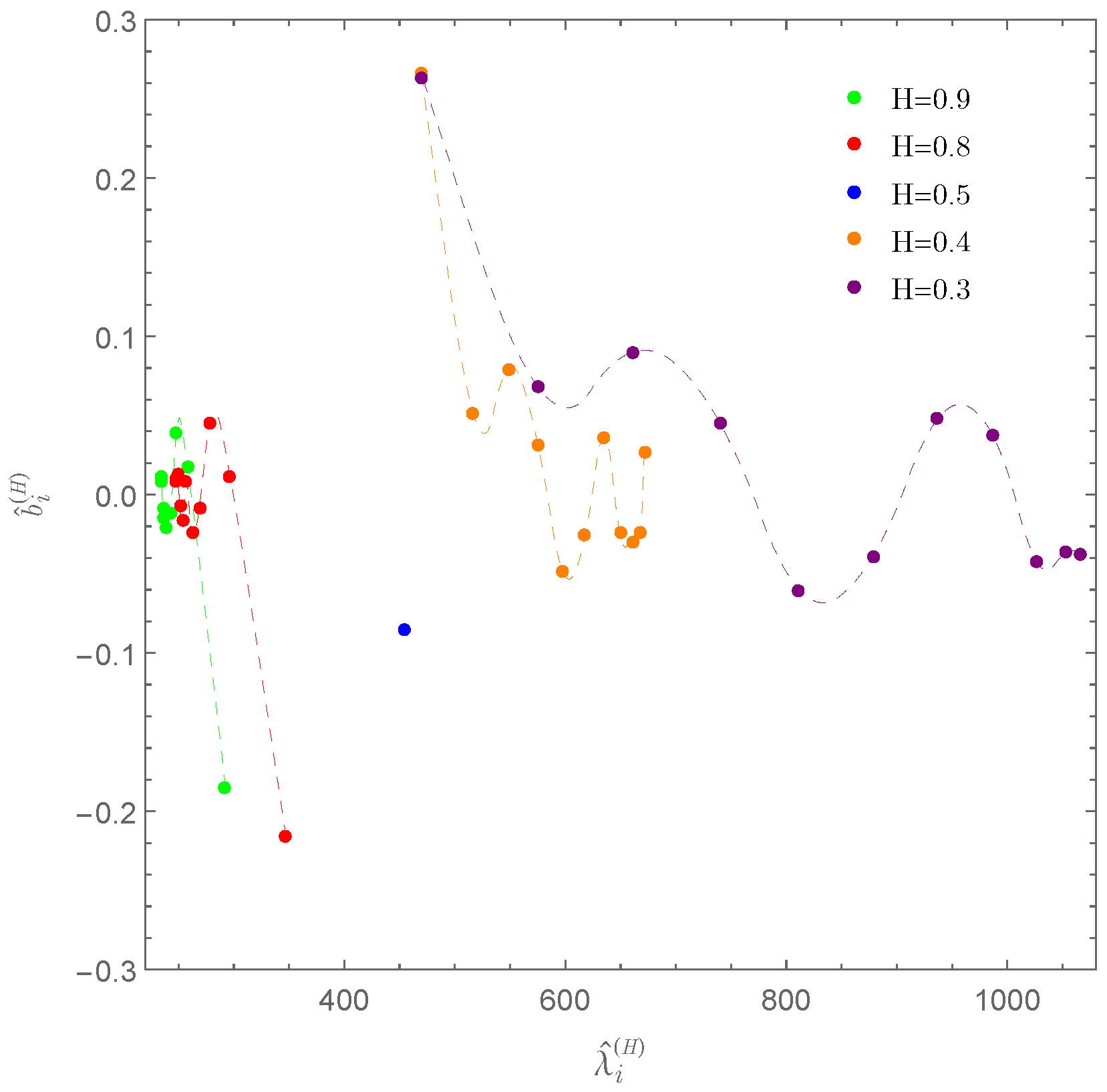
Figure 1 illustrates the pairs $\left({\widehat{\lambda }}_i^{\left(H\right)},{\widehat{b}}_i^{\left(H\right)}\right)$ associated with the matrix product ${\widehat{\mathit{A}}}_n{\widehat{\mathbf{\Sigma }}}_n^{\left(H\right)}$ for the selected Hurst parameters. The results demonstrate a clear sensitivity to changes in H. Specifically, lower values of H lead to a wider spread of eigenvalues with relatively larger magnitudes, which is consistent with the irregular and anti-persistent character of the increments. In contrast, as H approaches one, the eigenvalues exhibit an increasing concentration, reflecting smoother sample paths induced by strong positive dependence.

When the Hurst parameter is set to $H=0.5$, the driving noise reduces to standard Brownian motion. In this benchmark case, the matrix product ${\widehat{\mathit{A}}}_n{\widehat{\mathbf{\Sigma }}}_n^{\left(H\right)}$ simplifies to a diagonal matrix whose diagonal elements are all equal to

$${\displaystyle \frac{{100}^2}{T}}({\widehat{\sigma }}_B^2+{\widehat{\sigma }}_F^2)\Delta t.$$

Consequently, the spectral decomposition exhibits complete degeneracy, with all eigenvalues and their associated coefficients taking the same values, namely

$$\left({\widehat{\lambda }}_i^{\left(0.5\right)},{\widehat{b}}_i^{\left(0.5\right)}\right)\approx (454.545,-0.085),i=1,\dots ,n.$$

This uniform eigenstructure is a direct manifestation of the independent and stationary increment property characteristic of Brownian motion, and it provides a natural reference point against which the influence of long-memory and non-stationary effects can be assessed.

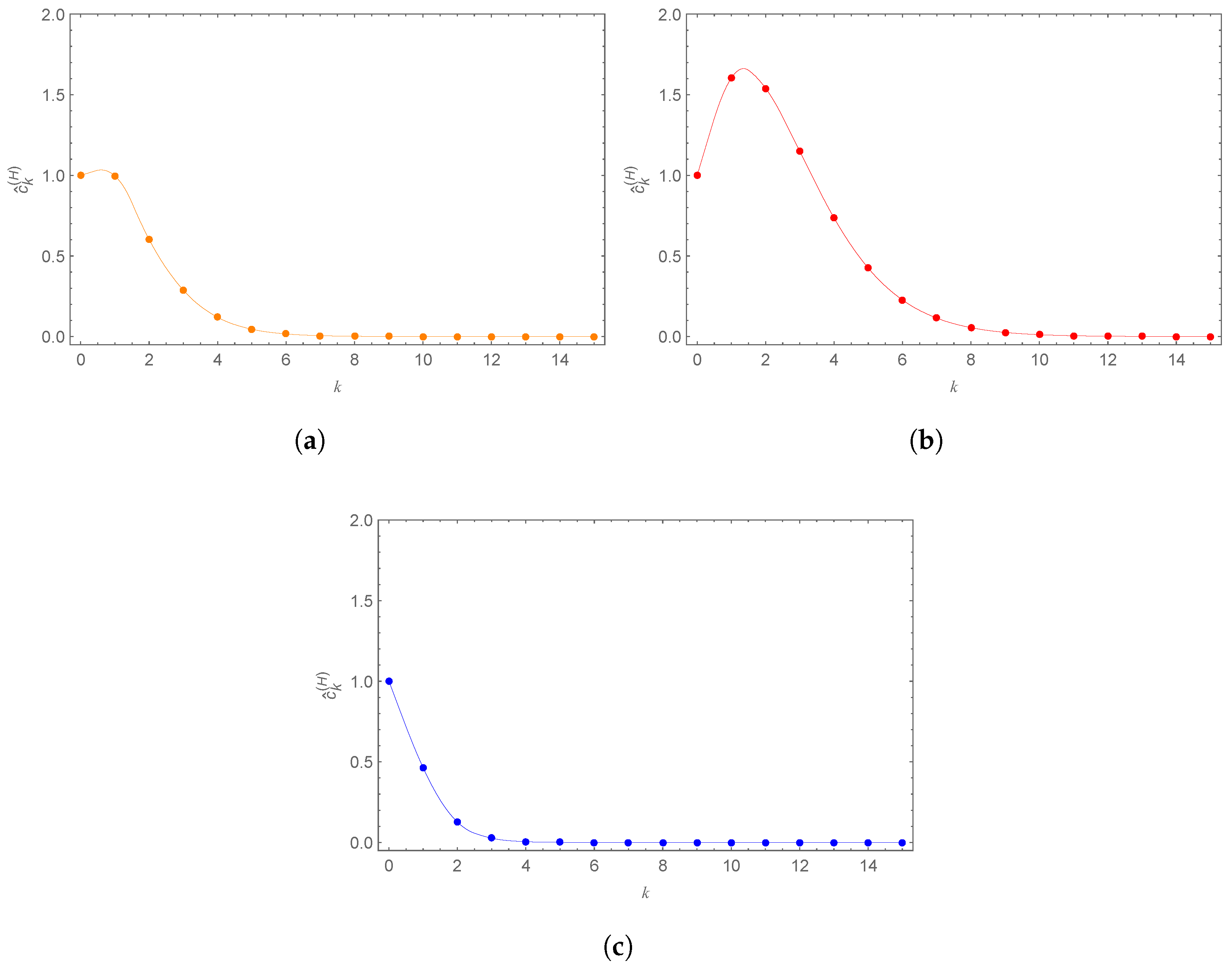
Under the admissibility condition (38) imposed on the scaling parameter β, the Laguerre expansion coefficients ${\widehat{c}}_k^{\left(H\right)}$ are evaluated via the recursive relations (31)–(33). Considering the illustrative choices $H=0.4$ and $H=0.8$, Figure 2a,b reveal a marked contrast in the rate of coefficient attenuation. In particular, the case corresponding to stronger persistence exhibits noticeably slower decay, indicating that long-memory effects materially influence both the regularity and the tail characteristics of the associated realized-variance distribution.

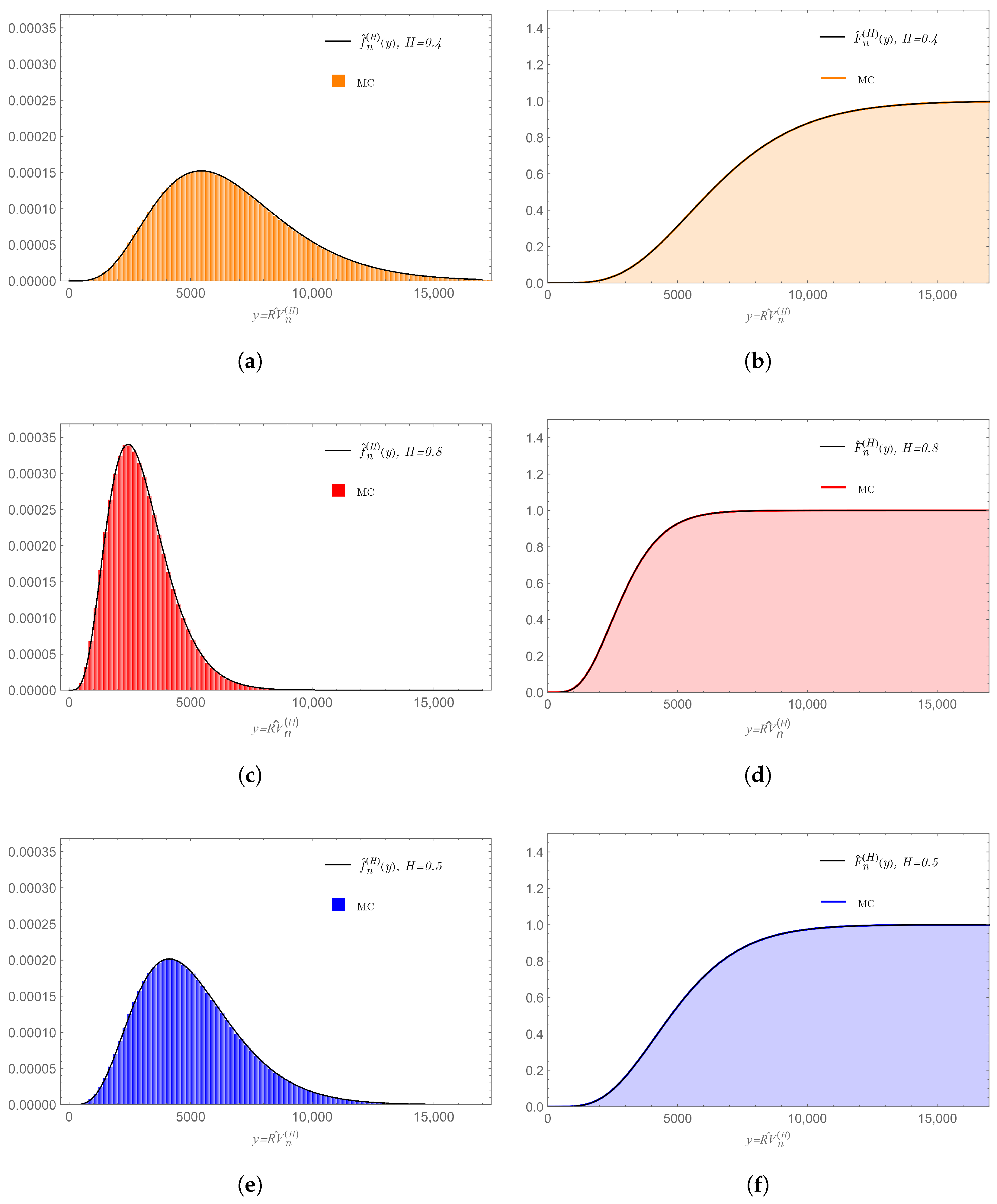
By inserting the numerically evaluated coefficients into the series representations (30) and (34), we obtain approximations of the probability density function and cumulative distribution function depicted in Figure 3. These analytical curves are benchmarked against MC histograms constructed from $5\times {10}^6$ independent realizations of ${\widehat{RV}}_n^{\left(H\right)}$, generated using the exact quadratic-form characterization (21)–(23). For all examined values of the Hurst parameter, the Laguerre-based approximations exhibit excellent agreement with the simulation results, thereby confirming both the numerical accuracy and the stability of the series expansions established in Theorems 6 and 7.

The special case $H=0.5$, corresponding to the classical Brownian setting, further illustrates the role of memory in the convergence behavior. As evidenced in Figure 2c, the associated Laguerre coefficients decrease at a much faster rate than in the fractional regimes, consistent with the lack of long-range dependence. The resulting density and distribution functions, shown in Figure 3e,f, display moderate dispersion and right-skewed profiles, placing the Brownian benchmark between the anti-persistent and persistent cases in terms of overall variability.

Taken together, these numerical findings underscore the central influence of the Hurst parameter on both the eigenstructure of the quadratic-form representation and the shape of the realized-variance distribution ${\widehat{RV}}_n^{\left(H\right)}$. Lower values of H lead to broader distributions with heavier tails, whereas higher values produce increasingly concentrated outcomes. The consistently close correspondence between the analytical Laguerre-series results and the MC simulations provides strong numerical support for the reliability and practical effectiveness of the proposed expansion methodology.

4.2. Analytical Valuation Versus MC Benchmarks

Example 26.

This experiment is designed to assess the numerical reliability of the closed-form pricing expressions developed in Section 3, focusing on both valuation precision and computational performance for volatility-dependent contracts. The analytical formulas are evaluated against MC simulation results under a fixed Hurst parameter $H=0.8$, corresponding to a strongly persistent dependence structure. All remaining model parameters coincide with those used in Example 25, ensuring comparability across numerical tests.

For conciseness, we present results for a representative collection of instruments, namely variance swaps, volatility swaps, variance put and call options, and volatility put and call options. These contracts collectively capture the essential features of the proposed pricing framework. Additional derivatives introduced in Section 3 have been examined in the same manner and exhibit consistent numerical behavior; their results are therefore omitted for brevity.

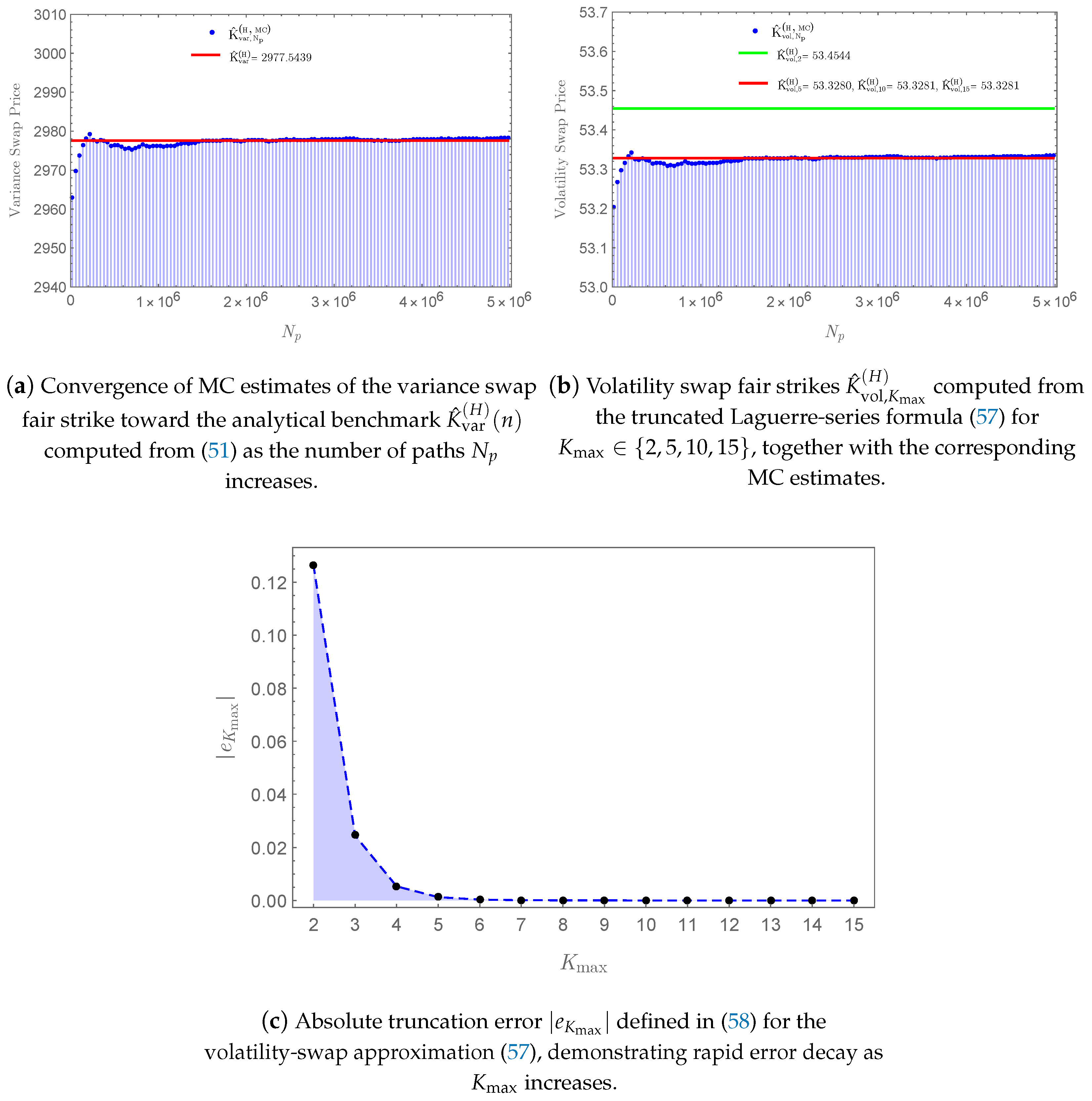
We first consider variance swap contracts. Figure 4a displays the analytical fair strike computed from the closed-form expression (51). To verify this theoretical value, we generate MC estimators ${\widehat{K}}_{\mathrm{var},N_p}^{(H,\mathrm{MC})}$ using progressively increasing sample sizes $N_p\in \{{10}^4,\dots ,5\times {10}^6\}$. As the number of simulated paths grows, the MC estimates exhibit clear convergence toward the analytical benchmark ${\widehat{K}}_{\mathrm{var}}^{\left(H\right)}\left(n\right)$, providing numerical confirmation of the validity and internal consistency of Formula (51).

Next, we turn to volatility swap contracts. Based on the Laguerre coefficient sequence ${\widehat{c}}_k^{\left(H\right)}$ (illustrated in Figure 2b), the fair volatility strike is approximated using the truncated expansion (57). Figure 4b displays the resulting estimates ${\widehat{K}}_{\mathrm{vol},K_{max}}^{\left(H\right)}$ for truncation levels $K_{max}=2,5,10,15$, alongside the corresponding MC reference values ${\widehat{K}}_{\mathrm{vol},N_p}^{(H,\mathrm{MC})}$. As the truncation order increases, the analytical approximation steadily approaches the simulation benchmark, with the choice $K_{max}=15$ yielding virtually identical values. This observation indicates that high numerical precision can be achieved without requiring excessively long series expansions. The absolute truncation error $|e_{K_{max}}|$, defined in (58), is plotted in Figure 4c and exhibits rapid decay, further corroborating the stability of the approximation.

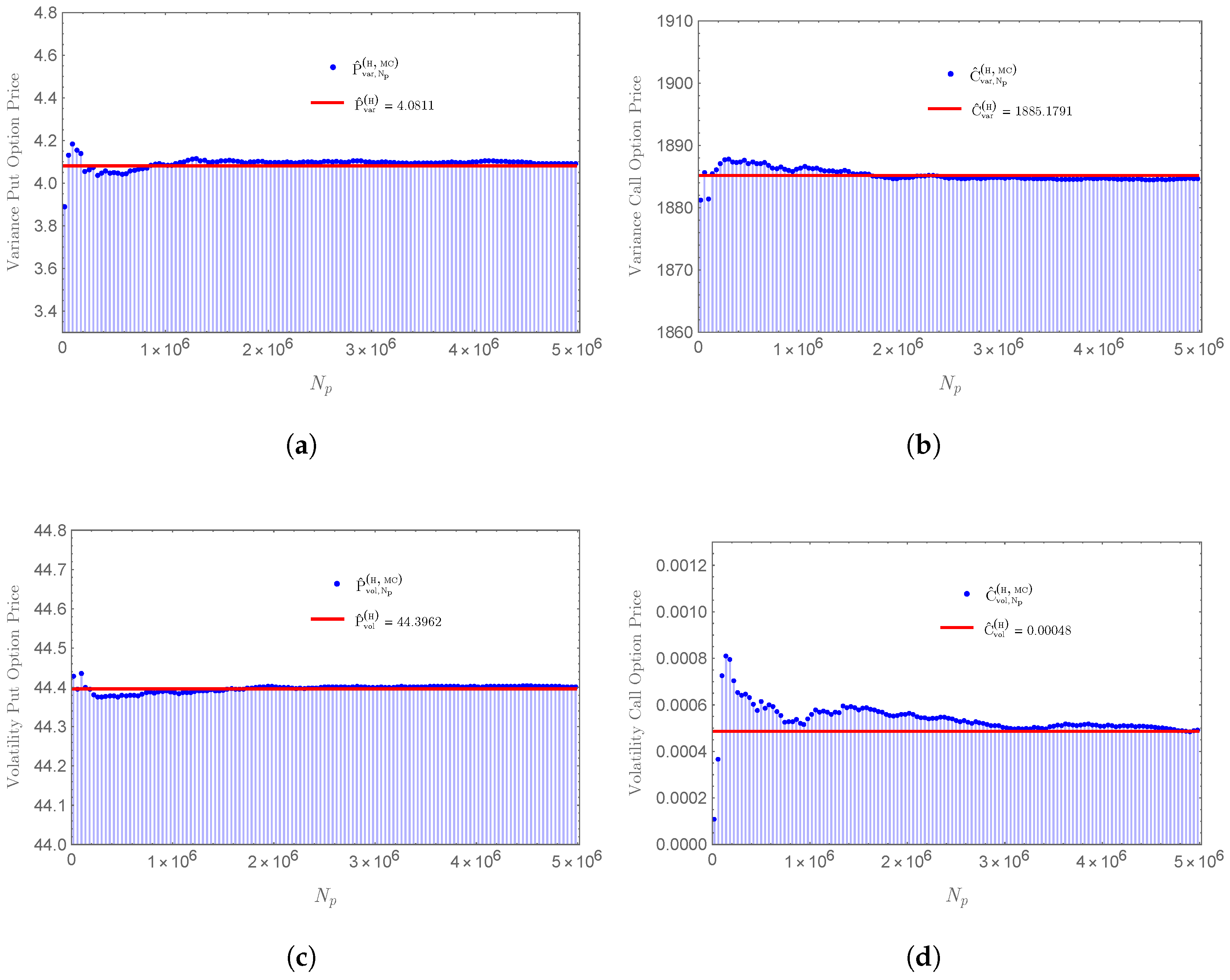
The analysis is subsequently extended to volatility derivatives with nonlinear payoffs, including variance and volatility options. For these products, pricing is carried out using the approximated cumulative distribution function of ${\widehat{RV}}_n^{\left(H\right)}$ (see Figure 3d). Figure 5a,b present MC price trajectories for variance put and call options with strike $K=1000$, together with the corresponding analytical values obtained from (67) and (69). Figure 5c,d report analogous results for volatility put and call options with strike $K=100$, computed using (74) and (76). Across all instruments considered, the MC estimators converge toward the analytical prices as the number of simulated paths increases, providing strong numerical support for the accuracy and robustness of the proposed valuation framework for both linear and nonlinear payoff structures.

We conclude this example by examining the computational performance of the two pricing approaches across the full set of six derivative contracts.

Table 2. Runtime and accuracy comparison between MC simulation and the proposed analytical valuation method for six volatility-linked contracts in Example 26 under $H=0.8$. For each product, the table reports the MC path count $N_p$, the percentage error $ϵ$ of the MC estimate relative to the analytical benchmark, the MC runtime $T^{\left(\mathrm{MC}\right)}$, the analytical runtime $T^{\left(\mathrm{E}\right)}$, and the speed-up factor (reduction).

Contract	${\mathit{N}}_{\mathit{p}}$	$\mathit{ϵ}$ (%)	${\mathit{T}}^{\left(\mathbf{MC}\right)}$ (s)	${\mathit{T}}^{\left(\mathbf{E}\right)}$ (s)	Reduction
Variance swaps
	$1\times {10}^4$	1.42	9.75	1.82	5
	$1\times {10}^5$	0.62	98.65	1.82	54
	$1\times {10}^6$	0.03	974.33	1.82	535
	$5\times {10}^6$	0.01	4850.27	1.82	2665
Volatility swaps
	$1\times {10}^4$	1.54	9.64	2.22	4
	$1\times {10}^5$	0.74	103.58	2.22	46
	$1\times {10}^6$	0.03	986.21	2.22	444
	$5\times {10}^6$	0.01	4996.24	2.22	2250
Variance put options
	$1\times {10}^4$	1.61	9.38	3.11	3
	$1\times {10}^5$	1.08	99.45	3.11	32
	$1\times {10}^6$	0.12	984.22	3.11	317
	$5\times {10}^6$	0.05	4871.01	3.11	1566
Variance call options
	$1\times {10}^4$	1.48	10.02	3.25	3
	$1\times {10}^5$	0.91	103.19	3.25	32
	$1\times {10}^6$	0.10	1007.51	3.25	310
	$5\times {10}^6$	0.03	4880.23	3.25	1501
Volatility put options
	$1\times {10}^4$	1.74	9.54	4.32	2
	$1\times {10}^5$	1.34	103.21	4.32	23
	$1\times {10}^6$	0.12	1010.30	4.32	233
	$5\times {10}^6$	0.03	4885.31	4.32	1130
Volatility call options
	$1\times {10}^4$	1.55	9.87	4.46	2
	$1\times {10}^5$	1.07	99.87	4.46	22
	$1\times {10}^6$	0.09	999.01	4.46	224
	$5\times {10}^6$	0.03	4872.44	4.46	1092

summarizes, for each instrument, the relative pricing error ϵ between MC estimates and the corresponding analytical values, the execution time required by the MC procedure $T^{\left(\mathrm{MC}\right)}$, the runtime of the analytical evaluation $T^{\left(\mathrm{E}\right)}$, and the implied acceleration factor. The results demonstrate that the analytical methodology delivers dramatic efficiency gains, often reducing computation time by several orders of magnitude for large values of $N_p$, while simultaneously preserving a high level of numerical accuracy (with all reported relative errors below $2\%$). The largest performance improvements are observed for variance swaps, where the analytical formulas yield speed-up factors exceeding 2600 when $N_p=5\times {10}^6$. These efficiency gains are especially advantageous in applications involving repeated valuation tasks, such as real-time pricing, high-frequency risk monitoring, large-scale scenario analysis, and fast model calibration.

4.3. Impact of the Hurst Parameter on Volatility Derivative Valuations

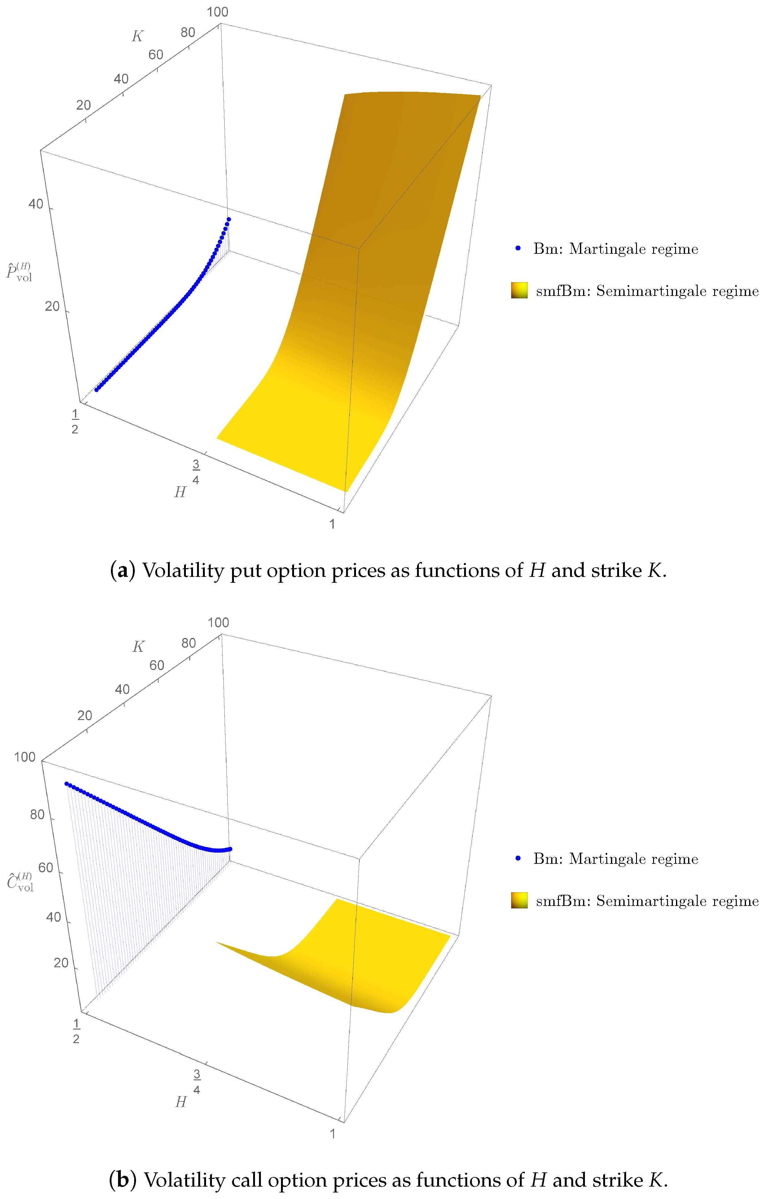
Example 27.

The parameter $H\in (0,1)$ governs the persistence properties and sample-path regularity of fractional-type Gaussian drivers, including the sfBm and related hybrid processes. Within the smfGBm dynamics (11), the prices of volatility-sensitive contracts are determined by the law of the discretely observed realized variance ${\widehat{RV}}_n^{\left(H\right)}$. As a consequence, both swap rates and option premia may exhibit pronounced dependence on the choice of H. This effect is of particular interest in the semimartingale region $H>\frac{3}{4}$, where the arbitrage-free and complete-market valuation framework remains valid despite the presence of correlated and non-stationary Gaussian increments.

To examine this dependence quantitatively, we evaluate variance swaps, volatility swaps, and volatility options using the closed-form pricing expressions derived in Section 3, fixing the contract maturity at $T=1$. For reference, the case $H=\frac{1}{2}$ serves as a baseline corresponding to the classical Brownian motion model with independent and stationary increments.

As illustrated in Figure 6a,b, the fair strike of variance swaps displays a strictly decreasing pattern as a function of H across all sampling schemes $N=12,52,252$. This monotonic behavior reflects the enhanced regularity and positive temporal dependence associated with larger values of H, which shift the mass of the realized-variance distribution toward lower outcomes and consequently reduce its expectation. A similar qualitative pattern is observed for volatility swaps, as shown in Figure 6c,d, where the corresponding fair strikes also decline with increasing H within the semimartingale range. However, the interaction with the sampling frequency is more intricate: while in the Brownian benchmark case, lower monitoring frequencies lead to smaller fair strikes, this ordering does not persist uniformly once long-memory effects become dominant, highlighting the combined influence of discretization and dependence structure.

For the remainder of this experiment, we restrict attention to the case $N=12$ and $T=1$ and focus on contracts with nonlinear payoff structures. Figure 7a,b reveal a clear asymmetry in the dependence of volatility option prices on the Hurst parameter. Specifically, volatility put prices rise as H increases, whereas the corresponding call prices exhibit a declining pattern. This behavior can be traced to a leftward shift in the distribution of ${\widehat{RV}}_n^{\left(H\right)}$ for larger values of H, which enhances the expected payoff of downside-protected contracts while diminishing that of upside-oriented positions. The magnitude of this sensitivity is most evident at lower strike levels and gradually weakens as H approaches unity, consistent with the increasing smoothness of the underlying sample paths.

Moreover, throughout the admissible semimartingale range with non-stationary increments, volatility put prices consistently exceed their Brownian reference values corresponding to $H=\frac{1}{2}$, while volatility call prices remain uniformly below this benchmark. This persistent ordering reflects the joint influence of temporal dependence and increment non-stationarity on the tail characteristics of ${\widehat{RV}}_n^{\left(H\right)}$, effects that are amplified for nonlinear payoff profiles relative to linear swap-based contracts.

Taken together, these numerical observations highlight the central importance of the Hurst parameter in determining volatility behavior and derivative pricing outcomes within the smfGBm framework (11). The combined roles of long-memory dependence, non-stationarity, and discretization frequency have direct consequences for valuation, hedging strategies, and risk assessment of volatility-related financial instruments.

5. Concluding Remarks

This study has introduced an integrated analytical approach for valuing a wide spectrum of volatility-related financial contracts within the sub-mixed fractional geometric Brownian motion (smfGBm) framework under discrete monitoring. The proposed model accommodates two empirically relevant features of asset return dynamics, namely temporal dependence and non-stationary Gaussian fluctuations, while retaining the semimartingale property necessary for arbitrage-free pricing when the Hurst parameter lies in the admissible range $H\in (\frac{3}{4},1)$.

A key methodological contribution of this paper is its explicit characterization of the distribution of discretely sampled log-return realized variance. By expressing this quantity as a quadratic form of correlated Gaussian increments with non-stationary structure, we obtained closed-form representations for both the probability density function and the cumulative distribution function through Laguerre-series expansions. These distributional results form the backbone of a tractable pricing framework that covers a broad family of volatility-linked instruments, including variance and volatility swaps, options written on realized variance or volatility, capped and floored products, knock-out contracts, and corridor-type structures with knock-out features.

The resulting analytical pricing expressions were subjected to extensive numerical testing using MC simulation benchmarks. Across all examined contracts, the analytical valuations closely matched the simulation results, even in regimes characterized by pronounced long-memory effects. At the same time, the proposed approach delivered dramatic gains in computational efficiency, with fast convergence and robust numerical behavior observed over a wide range of truncation levels, sampling schemes, and payoff specifications. These findings demonstrate that the Laguerre-based methodology provides a practical and reliable alternative to purely simulation-driven valuation techniques.

The numerical investigations further highlighted the decisive influence of the Hurst parameter on both the shape of the realized-variance distribution and the pricing of volatility-sensitive derivatives. Higher values of H lead to increasingly concentrated realized-variance distributions, which translate into systematically lower fair strikes for variance and volatility swaps. For derivatives with nonlinear payoffs, such as volatility options, the combined presence of long-memory dependence and non-stationary increments generates asymmetric pricing responses: option values for downside protection increase with H, whereas upside-oriented contracts exhibit declining prices. These patterns emphasize the necessity of incorporating long-range dependence and non-stationarity when modeling and managing volatility risk.

In summary, the framework developed herein provides a rigorous analytical toolkit for the valuation of volatility-linked derivatives in environments governed by correlated Gaussian processes with non-stationary and long-memory characteristics. Although the present work has focused on theoretical derivations and numerical performance, the relevance of the smfGBm dynamics is supported by existing empirical evidence documenting its improved descriptive power relative to standard and mixed fractional Brownian motion models. Against this empirical backdrop, the pricing formulas derived in this paper offer an efficient and transparent mechanism for volatility derivative valuation under realistic market dynamics. Natural avenues for future research include empirical calibration using market data, analysis of variance and volatility swap term structures, incorporation of jump components or regime-switching effects, multivariate extensions for joint volatility modeling, and applications to hedging design and volatility risk premia estimation based on high-frequency observations.

References

1. Broadie, M.; Jain, A. The effect of jumps and discrete sampling on volatility and variance swaps. Int. J. Theor. Appl. Financ. 2008, 11, 761–797. [Google Scholar] [CrossRef]
2. Xu, D.X.; Yang, B.Z.; Kang, J.H.; Huang, N.J. Variance and volatility swaps valuations with stochastic liquidity risk. Phys. A Stat. Mech. Its Appl. 2021, 566, 125679. [Google Scholar] [CrossRef]
3. Lin, S.; He, X.J. Analytically pricing variance and volatility swaps with stochastic volatility, stochastic equilibrium level and regime switching. Expert Syst. Appl. 2023, 217, 119592. [Google Scholar] [CrossRef]
4. Wu, B.; Chen, P.; Ye, W. Variance swaps with mean reversion and multi-factor variance. Eur. J. Oper. Res. 2024, 315, 191–212. [Google Scholar] [CrossRef]
5. Kim, H.G.; Kim, S.; Kim, J.H. Variance and volatility swaps and options under the exponential fractional Ornstein–Uhlenbeck model. N. Am. J. Econ. Financ. 2024, 72, 102155. [Google Scholar] [CrossRef]
6. Rujivan, S.; Rakwongwan, U. Analytically pricing volatility swaps and volatility options with discrete sampling: Nonlinear payoff volatility derivatives. Commun. Nonlinear Sci. Numer. Simul. 2021, 100, 105849. [Google Scholar] [CrossRef]
7. Rujivan, S. Valuation of volatility derivatives with time-varying volatility: An analytical probabilistic approach using a mixture distribution for pricing nonlinear payoff volatility derivatives in discrete observation case. J. Comput. Appl. Math. 2023, 418, 114672. [Google Scholar] [CrossRef]
8. Rujivan, S. Analytically pricing volatility options and capped/floored volatility swaps with nonlinear payoffs in discrete observation case under the Merton jump-diffusion model driven by a nonhomogeneous Poisson process. Appl. Math. Comput. 2025, 486, 129029. [Google Scholar] [CrossRef]
9. Castaño-Martínez, A.; López-Blázquez, F. Distribution of a sum of weighted noncentral chi-square variables. Test 2005, 14, 397–415. [Google Scholar] [CrossRef]
10. Rujivan, S.; Sutchada, A.; Chumpong, K.; Rujeerapaiboon, N. Analytically computing the moments of a conic combination of independent noncentral chi-square random variables and its application for the extended Cox–Ingersoll–Ross process with time-varying dimension. Mathematics 2023, 11, 1276. [Google Scholar] [CrossRef]
11. Ding, Z.; Granger, C.; Engle, R. A long memory property of stock market returns and a new model. J. Empir. Financ. 1993, 1, 83–106. [Google Scholar] [CrossRef]
12. Shiryaev, A. Essentials of Stochastic Finance: Facts, Models, Theory; World Scientific: Singapore, 1999. [Google Scholar]
13. Necula, C. Option pricing in a fractional Brownian motion environment. Adv. Econ. Financ. Res.—DOFIN Work. Pap. Ser. 2008, 2, 259–273. [Google Scholar] [CrossRef]
14. Kolmogorov, A. Wienersche spiralen und einige andere interessante kurven in hilbertscen raum, cr (doklady). Comptes Rendus (Dokl.) l’Académie Sci. l’URSS Nouv. Série 1940, 26, 115–118. [Google Scholar]
15. Chen, Q.; Zhang, Q.; Liu, C. The pricing and numerical analysis of lookback options for mixed fractional Brownian motion. Chaos Solitons Fractals 2019, 128, 123–128. [Google Scholar] [CrossRef]
16. Bian, L.; Li, Z. Fuzzy simulation of European option pricing using sub-fractional Brownian motion. Chaos Solitons Fractals 2021, 153, 111442. [Google Scholar] [CrossRef]
17. Wang, J.; Yan, Y.; Chen, W.; Shao, W.; Tang, W. Equity-linked securities option pricing by fractional Brownian motion. Chaos Solitons Fractals 2021, 144, 110716. [Google Scholar] [CrossRef]
18. Cheridito, P. Arbitrage in fractional Brownian motion models. Financ. Stoch. 2003, 7, 533–553. [Google Scholar] [CrossRef]
19. Bender, C.; Elliott, R. Arbitrage in a discrete version of the Wick-fractional Black-Scholes market. Math. Oper. Res. 2004, 29, 935–945. [Google Scholar] [CrossRef]
20. Björk, T.; Hult, H. A note on Wick products and the fractional Black-Scholes model. Financ. Stoch. 2005, 9, 197–209. [Google Scholar] [CrossRef]
21. Bojdecki, T.; Gorostiza, L.; Talarczyk, A. Sub-fractional Brownian motion and its relation to occupation times. Stat. Probab. Lett. 2004, 69, 405–419. [Google Scholar] [CrossRef]
22. Angstmann, C.; Henry, B.I.; McGann, A. Time-fractional geometric Brownian motion from continuous time random walks. Phys. A Stat. Mech. Its Appl. 2019, 526, 121002. [Google Scholar] [CrossRef]
23. Stojkoski, V.; Sandev, T.; Basnarkov, L.; Kocarev, L.; Metzler, R. Generalised geometric Brownian motion: Theory and applications to option pricing. Entropy 2020, 22, 1432. [Google Scholar] [CrossRef]
24. Alazemi, F.; Alsenaf, A.; Najafi, A. A spectral approach using fractional Jaiswal functions to solve the mixed time-fractional Black–Scholes European option pricing model with error analysis. Numer. Algorithms 2025, 98, 347–371. [Google Scholar] [CrossRef]
25. Tudor, C. Some properties of the sub-fractional Brownian motion. Stochastics 2007, 79, 431–448. [Google Scholar] [CrossRef]
26. Wang, W.; Cai, G.; Tao, X. Pricing geometric asian power options in the sub-fractional Brownian motion environment. Chaos Solitons Fractals 2021, 145, 110754. [Google Scholar] [CrossRef]
27. El-Nouty, C. The fractional mixed fractional Brownian motion. Stat. Probab. Lett. 2003, 65, 111–120. [Google Scholar] [CrossRef]
28. Mishura, Y.S. Stochastic Calculus for Fractional Brownian Motion and Related Processes; Springer Press: Berlin, Germany, 2008. [Google Scholar]
29. Cheridito, P. Mixed fractional Brownian motion. Bernoulli 2001, 7, 913–934. [Google Scholar] [CrossRef]
30. Charles, E.; Mounir, Z. On the sub-mixed fractional Brownian motion. Appl. Math. A J. Chin. Univ. 2015, 30, 27–43. [Google Scholar] [CrossRef]
31. Xu, F.; Zhou, S. Pricing of perpetual American put option with sub-mixed fractional Brownian motion. Fract. Calc. Appl. Anal. 2019, 22, 1145–1154. [Google Scholar] [CrossRef]
32. Ji, B.; Tao, X.; Ji, Y. Barrier option pricing in the sub-mixed fractional Brownian motion with jump environment. Fractal Fract. 2022, 6, 244. [Google Scholar] [CrossRef]
33. Guo, J.; Kang, W.; Wang, Y. Option pricing under sub-mixed fractional Brownian motion based on time-varying implied volatility using intelligent algorithms. Soft Comput. 2023, 27, 15225. [Google Scholar] [CrossRef]
34. Guo, J.; Wang, Y.; Kang, W. European vulnerable options pricing under sub-mixed fractional jump-diffusion model with stochastic interest rate. Commun. Stat.—Simul. Comput. 2024, 1–35. [Google Scholar] [CrossRef]
35. Ma, P.; Najafi, A.; Gomez-Aguilar, J. Sub mixed fractional Brownian motion and its application to finance. Chaos Solitons Fractals 2024, 184, 114968. [Google Scholar] [CrossRef]
36. Zhang, W.; He, G.; Lou, M.; Liang, W. Valuation of R&D projects of new energy vehicles based on generalized mixed sub-fractional Brownian motion under fuzzy environment. Appl. Math. Comput. 2025, 507, 129559. [Google Scholar]
37. Rujivan, S. Analytical valuation of nonlinear payoff volatility derivatives with discrete sampling under a mixed fractional geometric Brownian motion model. Commun. Nonlinear Sci. Numer. Simul. 2026, 156, 109626. [Google Scholar] [CrossRef]
38. Mathai, A.; Provost, S. Quadratic Forms in Random Variables, Statistics: A Series of Textbooks and Monographs; CRC Press: Boca Raton, FL, USA, 1992. [Google Scholar]
39. Thamrongrat, N.; Chhum, C.; Rujivan, S.; Djehiche, B. An analytical formula for the transition density of a conic combination of independent squared Bessel processes with time-dependent dimensions and financial applications. Mathematics 2025, 13, 2106. [Google Scholar] [CrossRef]
40. Szegö, G. Orthogonal Polynomials; American Mathematical Society: Providence, RI, USA, 1939; Volume 23. [Google Scholar]
Figure 1. Eigenvalue–coefficient pairs λ ^ i ( H ) , b ^ i ( H ) corresponding to the matrix product A ^ n Σ ^ n ( H ) for selected Hurst parameters H = 0.3 , 0.4 , 0.5 , 0.8 , and 0.9 , with T = 1 and n = 11 as specified in Example 25. Greater eigenvalue dispersion for H 0 reflects rough, anti-persistent paths, while increased concentration for H 1 indicates smoother, persistent dynamics. At H = 0.5 , the matrix is diagonal with constant pairs ( λ ^ i ( 0.5 ) , b ^ i ( 0.5 ) ) ( 454.545 , 0.085 ) , reflecting independent and stationary increments.
Fractalfract 10 00125 g001
Figure 2. Laguerre coefficients c ^ k ( H ) for selected Hurst parameters H = 0.4 , 0.8 , and 0.5 , as examined in Example 25. (a) Coefficients in the Laguerre series expansion for H = 0.4 . (b) Coefficients in the Laguerre series expansion for H = 0.8 . (c) Coefficients in the Laguerre series expansion for H = 0.5 .
Fractalfract 10 00125 g002
Figure 3. Laguerre-based PDF and CDF approximations of R V ^ n ( H ) compared with MC simulations for selected Hurst parameters H = 0.4 , 0.8 , and 0.5 , as examined in Example 25. (a) Approximate PDF of R V ^ n ( H ) vs. MC simulations for H = 0.4 . (b) Approximate CDF of R V ^ n ( H ) vs. MC simulations for H = 0.4 . (c) Approximate PDF of R V ^ n ( H ) vs. MC simulations for H = 0.8 . (d) Approximate CDF of R V ^ n ( H ) vs. MC simulations for H = 0.8 . (e) Approximate PDF of R V ^ n ( H ) vs. MC simulations for H = 0.5 . (f) Approximate CDF of R V ^ n ( H ) vs. MC simulations for H = 0.5 .
Fractalfract 10 00125 g003
Figure 4. Accuracy and convergence diagnostics for swap contracts under the smfGBm model with H = 0.8 in Example 26: (a) MC convergence for the variance-swap fair strike; (b) volatility-swap fair strikes from the truncated Laguerre formula (57) compared with MC; and (c) truncation-error decay for (57).
Fractalfract 10 00125 g004
Figure 5. Convergence of MC prices toward the analytical benchmarks for nonlinear volatility derivatives under the smfGBm model with H = 0.8 in Example 26: variance put/call options priced via (67) and (69) (strike K = 1000 ), and volatility put/call options priced via (74) and (76) (strike K = 100 ). (a) Variance put option: MC price convergence to the analytical price computed from (67) with strike K = 1000 . (b) Variance call option: MC price convergence to the analytical price computed from (69) with strike K = 1000 . (c) Volatility put option: MC price convergence to the analytical price computed from (74) with strike K = 100 . (d) Volatility call option: MC price convergence to the analytical price computed from (76) with strike K = 100 .
Fractalfract 10 00125 g005
Figure 6. Sensitivity of swap fair strikes to the Hurst parameter H under the smfGBm model (11) in Example 27. Panels (a,b) show variance swap strikes for sampling frequencies N { 12 , 52 , 252 } , which decrease monotonically with H. Panels (c,d) report volatility swap strikes, which also decline with H in the semimartingale regime, while exhibiting a regime-dependent dependence on N.
Fractalfract 10 00125 g006
Figure 7. Sensitivity of volatility option prices to the Hurst parameter H { 1 2 } ( 3 4 , 1 ) under the smfGBm model (11) in Example 27 with T = 1 and N = 12 . As H increases, put prices rise while call prices fall, reflecting a shift in the distribution of R V ^ n ( H ) toward smaller values. In the semimartingale regime, volatility put prices are uniformly above—and volatility call prices uniformly below—their Brownian benchmark values at H = 1 2 .
Fractalfract 10 00125 g007