Optimal Fractional Order PID Controller Design for Hydraulic Turbines Using a Multi-Objective Imperialist Competitive Algorithm

Abstract

This paper introduces a novel approach for designing a Fractional Order Proportional-Integral-Derivative (FOPID) controller for the Hydraulic Turbine Regulating System (HTRS), aiming to overcome the challenge of tuning its five complex parameters ($K_p,K_i,K_d$, λ and μ). The design is formulated as a multi-objective optimization problem, minimized using the Multi-Objective Imperialist Competitive Algorithm (MOICA). The goal is to minimize two key transient performance metrics: the Integral of Squared Error (ISE) and the Integral of the Time Multiplied Squared Error (ITSE). MOICA efficiently generates a Pareto-front of non-dominated solutions, providing control system designers with diverse trade-off options. The resulting optimal FOPID controller demonstrated superior robustness when evaluated against simulated variations in key HTRS parameters (mg, eg and Tw). Comparative simulations against an optimally tuned integer-order PID and established literature methods (FOPID-GA, FOPID-MOPSO and FOPID-MOHHO) confirm the enhanced dynamic response and stable operation of the MOICA-based FOPID. The MOICA-tuned FOPID demonstrated superior performance for Setpoint Tracking, achieving up to a 26% faster settling speed (ITSE) and an 8% higher accuracy (ISE). Furthermore, for Disturbance Rejection, it showed enhanced robustness, leading to up to a 23% quicker recovery speed (ITSE) and an 18.9% greater error suppression (ISE).

1. Introduction

HTRS is a complex engineering plant that integrates hydraulic, mechanical, and electrical dynamics. The performance of the turbine governor, which controls the hydroelectric generating unit (HGU), is crucial for maintaining power grid efficiency and stability. For decades, the simplicity of the conventional Proportional-Integral-Derivative (PID) controller made it the industry’s default choice [1].

Escalating demands for faster dynamic response and improved robustness have driven researchers toward advanced control architectures, notably the Fractional-Order PID (FOPID) controller. Derived from fractional calculus, the FOPID generalizes the standard PID by introducing non-integer orders for the derivative (μ) and integral (λ) components. This expanded structure offers two additional degrees of freedom, providing FOPID with greater flexibility and robustness than its integer-order counterpart [2].

The FOPID controller’s inherent stability and dynamic performance have facilitated its widespread adoption across diverse engineering disciplines and complex industrial plants globally. Studies confirm its effectiveness in power generation [3,4,5,6], motion control [7,8,9], and specialized industrial processes [10,11,12].

Despite these benefits, the introduction of two supplementary parameters into the FOPID structure elevates the tuning process to a significant challenge. This controller expands on the conventional three-parameter PID structure. It requires the simultaneous optimization of five parameters: the proportional, integral, and derivative gains ($K_p,{ K}_i,{ K}_d$), plus the integration (λ) and differentiation (μ) orders. This intricacy necessitates the use of powerful optimization methodologies [13,14,15].

A wide array of methods has been documented for FOPID parameter tuning, broadly falling into two categories. Analytical and rules-based approaches focus on structured design. These include techniques using piecewise orthogonal function expansion [16] and rule sets based on first-order plus dead-time models to constrain sensitivity [17]. Other designs prioritize enforcing specific gain and phase margin specifications [18]. The second, more recent category involves leveraging intelligent evolutionary algorithms to navigate the complex, five-dimensional parameter space. Notable examples of this strategy include the use of Particle Swarm Optimization (PSO) [19], the Genetic algorithm [20], and advanced versions of the Differential Evolution algorithm [21,22,23,24].

Despite these advancements, most of the existing research remains focused on single-objective design strategies. In contrast, practical control systems, particularly the Hydraulic Turbine Regulating System (HTRS), inherently require a balance between several conflicting performance indicators. Tuning FOPID controllers for HTRS remains a significant challenge due to the high-dimensional search space and the system’s non-linear dynamics. While multi-objective optimization has been validated as effective for managing such trade-offs [25,26,27], a critical gap remains in applying high-performance socio-political algorithms to this specific framework.

To address this, this paper presents a novel application of the Multi-Objective Imperialist Competitive Algorithm (MOICA), specifically the variant augmented with attractive and repulsive assimilation phases [28,29]. Unlike bio-inspired methods such as NSGA-II or MOPSO, MOICA is grounded in socio-political competition, offering unique structural advantages for the HTRS environment. First, its dual-phase assimilation process prevents premature convergence in the five-parameter space. Second, its competitive empire dynamics utilize a power-sharing mechanism to eliminate weak solutions, accelerating the search for global optima. Finally, by combining fast non-dominated sorting with colonial evolution, MOICA maintains a highly diverse external archive, resulting in a superior Pareto front [28,29].

In this study, the MOICA is strategically deployed to identify the optimal trade-offs between two conflicting indices: Integral Square Error (ISE) and Integral Time Square Error (ITSE). While ISE-based solutions typically favor stability and low overshoot, ITSE-based solutions prioritize response speed [30]. The primary novelty of this research lies in the synergy between MOICA’s exploration capabilities and the non-linear dynamics of hydraulic turbines, establishing a new benchmark for robust governor design. To validate this approach, rigorous comparative simulations were conducted against optimally tuned integer-order PID controllers and established literature methods (e.g., FOPID-GA, FOPID-MOHHO, and FOPID-MOPSO). The findings demonstrate that the MOICA-based FOPID approach provides significantly enhanced dynamic response and stability compared to all baseline and previously published controllers.

2. HTRS Modeling and FOPID Controller Background

2.1. HTRS Modeling

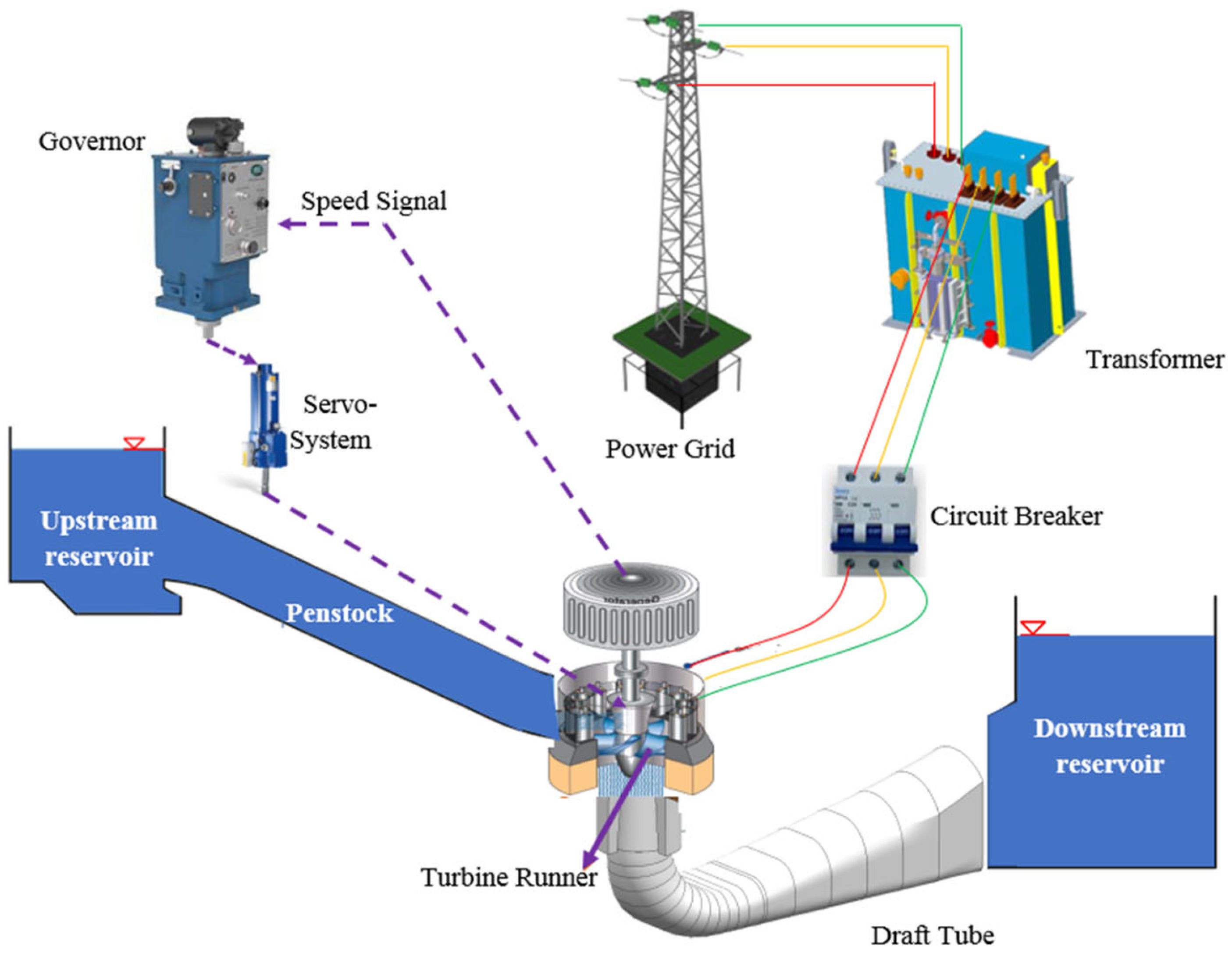
The HTRS begins with the Upstream Reservoir, which stores the water’s potential energy. This water is then conveyed as high-pressure flow through the Penstock to the Turbine. The turbine converts hydraulic energy into rotational mechanical power. This power is then transmitted to the generator and converted into electrical energy. Finally, the voltage is stepped up by a transformer and fed into the power grid through a circuit breaker [31].

As presented in Figure 1, the core of the control is the electric governor, which constantly monitors the speed signal to detect any deviation from the desired setpoint. When a change in electrical load causes the frequency to drop, the governor calculates the necessary corrective action using its control algorithm. It then sends a command signal to the Servosystem, which uses high-pressure fluid to rapidly and precisely adjust the position of the turbine’s internal gates (or wicket vanes). This movement modulates the water flow from the penstock to the turbine. This adjusts the mechanical power output to match the grid load and restores the frequency to its stable setpoint. The regulation cycle completes as the water is discharged into the downstream reservoir.

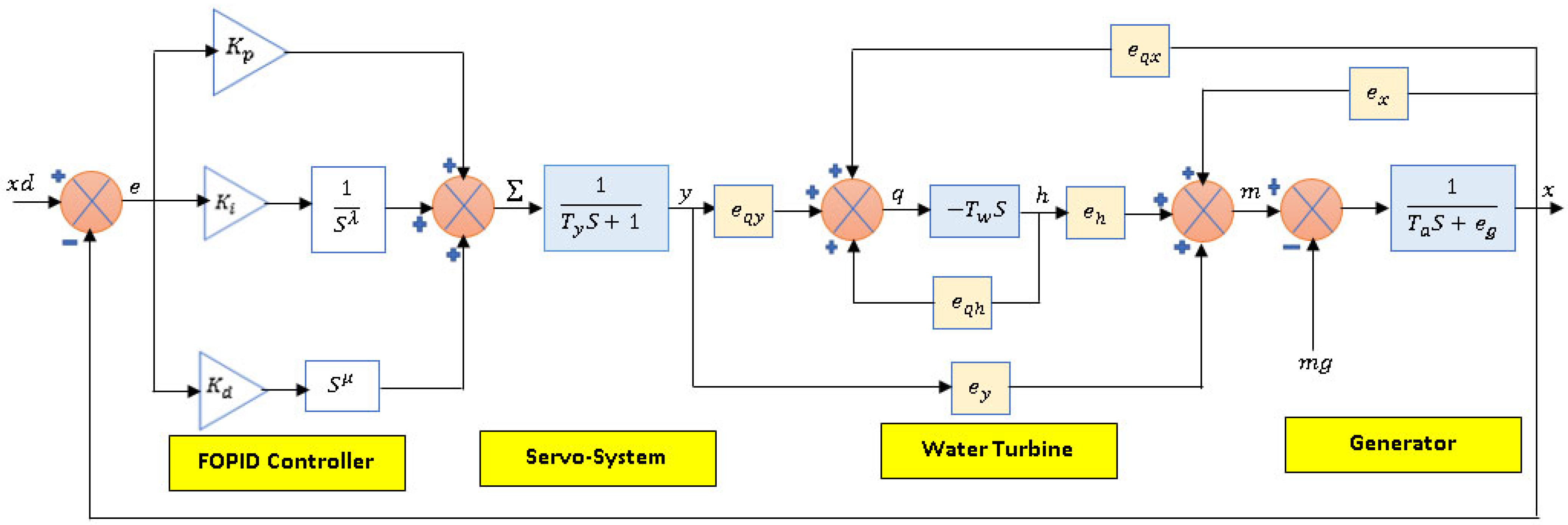
The general layout of the HTRS is presented in Figure 2, which consists of four main functional blocks.

The electro-hydraulic servosystem serves as the turbine’s actuator. It uses auxiliary relay connectors to amplify electrical signals, generating the hydraulic force needed to adjust the wicket vanes. Due to the significantly faster response of the auxiliary relay, its dynamics are considered negligible relative to the major relay. This disparity allows the entire servomechanism to be simplified into a first-order model, yielding the following transfer function [31]:

$$F_S\left(S\right)={\displaystyle \frac{1}{T_{y}S+1}}$$

(1)

where $T_y$ represents the Time constant of the major relay.

The flow and torque of hydraulic turbines are inherently nonlinear functions, described as follows:

$$\mathrm{m} = f_1\left(x,y.h\right)$$

(2)

$$\mathrm{q}=f_2\left(x,y.h\right)$$

(3)

where x denotes the relative speed turbine deviation. y is the wicket gate stroke relative deviation and h represents the water head relative deviation.

For control design purposes, these dynamics (Equations (2) and (3)) are linearized using a first-order Taylor series expansion around some steady-state working conditions. This results in the linear turbine Equations (4) and (5) [22,32,33,34,35]:

$${m=e_{x}x+e_{y}y+e}_h\mathrm{h}$$

(4)

$${q=e_{qx}x+e_{qy}y+e}_{qh}\mathrm{h}$$

(5)

The parameters $e_x, { e}_y \mathrm{a}\mathrm{n}\mathrm{d} e_h$ represent the turbine torque transfer coefficients relative to rotational speed, guide vane opening, and water head, respectively. Similarly, $e_{qx}, e_{qy} \mathrm{a}\mathrm{n}\mathrm{d} e_{qh}$ denote the turbine flow transfer coefficients relative to rotational speed, guide vane opening, and water head.

The hydraulic turbine, the core of the HTRS, is a complex system typically analyzed as two interacting subsystems: the turbine and the penstock pipeline. Modeling fluid dynamics within the penstock is challenging due to non-linear flow-pressure relationships. To facilitate control design, the model is linearized by assuming rigid water column dynamics and constant plant parameters. These simplifications allow the water hammer effect to be approximated by the following transfer function [32]:

$$F_T\left(S\right)={\displaystyle \frac{h\left(S\right)}{q\left(S\right)}}=-T_{w}S$$

(6)

where $h\left(S\right)$ and $q\left(S\right)$ represent the Laplace transform of water head and flow rate relative deviations, respectively. $T_w$ denotes the water starting time constantly.

The generator’s dynamics system’s behavior is simplified for the simulation and expressed by the following standard transfer function [32].

$$F_g\left(S\right)={\displaystyle \frac{x\left(S\right)}{m\left(S\right)-mg\left(S\right)}}={\displaystyle \frac{1}{T_{a}S+e_g}}$$

(7)

$T_a$ is the generator mechanical time constant, while $e_g$ is the load self-regulation parameter. $x\left(S\right)$ and $mg\left(S\right)$ are the Laplace transform of turbine speed and load torque relative deviations, respectively.

2.2. FOPID Controller

The PID is currently the most prevalent form of governor used within the HTRS. However, in this work, we propose replacing the conventional PID controller with the more advanced FOPID controller within the HTRS architecture. The FOPID is an extension of the conventional PID where the integral and derivative operations are defined using the principles of fractional calculus. This results in a control system whose dynamics are governed by the following differential equation in the time domain [33]:

$$u\left(t\right)=K_{p}e\left(t\right)+K_i{D}^{-\lambda }e\left(t\right)+K_d{D}^{\mu }e\left(t\right)$$

(8)

This equation defines the FOPID controller’s output u(t) based on the error e(t), where $K_p, K_i \mathrm{and} K_d$ are the proportional, integral, and derivative gains, respectively. $D^{-\lambda }$ represents the fractional integral of order λ and $D^{\mu }$ represents the fractional derivative of order μ. The transfer function for the FOPID is derived by applying the Laplace transform to its time-domain differential equation, resulting in the following expression [33]:

$$C\left(S\right)=K_p+{\displaystyle \frac{K_i}{S^{\lambda }}}+K_d{S}^{\mu }$$

(9)

The closed-loop configuration of the HTRS utilizing the FOPID controller is illustrated in Figure 3, which clearly depicts the interconnection of the controller’s transfer function with the HTRS plant model.

For the numerical simulation and practical realization of the FOPID controller, the fractional operators $S^{\mathsf{\lambda }}$ and $S^{\mu }$ are approximated using Oustaloup’s band-limited frequency domain approximation technique. This technique involves the recursive distribution of N poles and N zeros of the following form, to construct a higher-order analog filter [19,21,22].

$$S^{\alpha }=K\prod _{i=-N}^N{\displaystyle \frac{S+{\omega }_i^{\prime }}{S+{\omega }_i}}$$

(10)

The filter’s poles, zeros, and gain are determined through a recursive evaluation process, defined as

$${\omega }_i={\omega }_b{\left({\displaystyle \frac{{\omega }_h}{{\omega }_b}}\right)}^{{\displaystyle \frac{i+N+\frac{1}{2}\left(1+\alpha \right)}{2N+1}}}, {\omega }_i^{\prime }={\omega }_b{\left({\displaystyle \frac{{\omega }_h}{{\omega }_b}}\right)}^{{\displaystyle \frac{i+N+\frac{1}{2}\left(1-\alpha \right)}{2N+1}}}, {K=\omega }_h^{\alpha }$$

$\alpha$ denotes the order of the fractional integro-differential operator, (2N + 1) represents the resulting order of the analog filter, and ${(\omega }_b,{\omega }_h)$ specifies the targeted frequency range for the approximation.

In this study, to ensure high fidelity and reproducibility, a 5th-order approximation (N = 5) was employed within a frequency range of [10⁻², 10²] rad/s. This range is chosen as it effectively covers the dominant dynamics of the HTRS while maintaining numerical stability [19,21,22].

The detailed HTRS model and the flexible FOPID structure emphasize a core challenge. Specifically, designers must optimize five parameters ($K_p,K_i,K_d$, λ and μ) while balancing conflicting performance goals. The next section, Optimization Problem Formulation, formally defines the design variables and constraints. It also establishes the objective functions required to solve this complex, multi-objective challenge.

3. Multi-Objective Optimization Problem Formulation

The multi-objective optimization problem for the HTRS FOPID controller is mathematically formulated to find the ideal compromise between competing goals. This formulation ensures optimal performance while strictly adhering to physical constraints.

This formulation seeks to minimize two primary, conflicting objective functions by intelligently searching for the optimal five FOPID parameters. The problem is expressed as finding the vector of design variables (DVs) that minimizes two objective functions F1(DVs) and F2(DVs), subject to a set of constraints.

3.1. Design Variables and Constraints

The vector of decision variables (DVs) consists of the five adjustable parameters of the FOPID controller: the three gains and the two fractional orders.

$$\mathbf{DVs}=[K_p,K_i, K_d, \lambda , \mu ]$$

(11)

To ensure the controller is physically realizable and to maintain system stability, the search space is constrained as defined in

Table 1. Feasible ranges of design variables.

DVs	${\mathit{K}}_{\mathit{p}}$	${\mathit{K}}_{\mathit{i}}$	${\mathit{K}}_{\mathit{d}}$	λ	μ
Range	[0, 15]	[0, 15]	[0, 15]	[0, 2]	[0, 2]

.

3.2. Objective Functions (Performance Metrics)

The goal of the multi-objective optimization is to find the Pareto-optimal set that minimizes the following two time-domain performance indices simultaneously:

Objective 1: Minimize Integral of Squared Error (ISE)

The ISE objective favors a design with a small overshoot and high stability, though it may result in a slower response. The error e(t) is typically the deviation of the generator speed from its setpoint.

Minimize F1(DVs) = ISE = ${\int }_0^{\infty }{e}^2\left(t\right)dt$

Objective 2: Minimize Integral of Time Multiplied Squared Error (ITSE)

The ITSE objective penalizes large errors that occur later in the transient response, thus promoting a faster settling time and speedier elimination of the transient error.

Minimize F2(DVs) = ITSE = ${\int }_0^{\infty }{te}^2\left(t\right)dt$

For the control loop to operate effectively, both objective functions (F1 and F2) must be simultaneously minimized. The Integral Squared Error (ISE) represents a fundamental design trade-off. Minimizing it encourages the control system to act faster and stabilize error magnitudes quickly. This objective typically favors designs with small overshoot. However, this pursuit of speed and low initial error can sometimes lead to a longer settling time. In contrast, minimizing the Integral Time Squared Error (ITSE) penalizes errors that persist late in the response. This is due to the multiplying time factor (t), which effectively forces a shorter settling time.

System stability is explicitly ensured through the optimization process. By minimizing the ITSE objective function, the algorithm applies a heavy mathematical penalty to errors that persist or grow over time. Consequently, any parameter sets leading to instability or sustained oscillations are naturally eliminated by the MOICA, as they yield high ITSE values, ensuring that only robustly stable solutions reach the final Pareto front.

4. Multi-Objective Imperialist Competitive Algorithm (MOICA)

The Multi-Objective Imperialist Competitive Algorithm (MOICA) is a recently developed evolutionary optimization method introduced by [28], which is fundamentally derived from the original Imperialist Competitive Algorithm (ICA) [34]. The pseudocode of the MOICA is illustrated in Figure 4. The subsequent text details the specific operational steps of the MOICA.

Step 1: Initialize country and evaluate the empires

The MOICA begins by randomly generating an initial population of countries. Each individual country within this population represents a potential design vector (DVs), which in this context holds a specific set of FOPID parameters. The cost associated with any country is determined by evaluating the objective functions (F1(DVs) = ISE and F2(DVs) = ITSE) using that country’s DVs. The country with the overall lowest cost (best performance) is designated the “imperialist,” while all other countries are considered “colonies.” The normalized cost of the nth imperialist is subsequently calculated using the following formula:

$$C_n=\underset{i}{max}\left\{Cos{t}_i\right\}-Cos{t}_n$$

(12)

$$Cos{t}_n=\sum _{j=1}^r{\displaystyle \frac{\left|F_{j,n}-F_j^{best}\right|}{\left|F_j^{max}-F_j^{min}\right|}}$$

(13)

where $Cos{t}_i$ and $Cos{t}_n$ are the cost of the i^th and the nth imperialist, respectively. r is the number of objective functions and $F_{j,n}$ is the value of objective function j for imperialist n. $F_j^{best}$, $F_j^{\mathit{max}}$ and $F_j^{\mathit{min}}$ are the best, maximum and minimum values of objective function j in each iteration, respectively [28,29,36].

The normalized power of the nth imperialist is calculated using the following expression:

$$P_n=\left|{\displaystyle \frac{C_n}{{\sum }_i{C}_i}}\right|$$

(14)

Once the normalized power of each imperialist is determined, the initial empires are formed. Each newly formed empire consists of one designated imperialist and a specific number of assigned colonies. Critically, the number of colonies each imperialist receives is directly proportional to its calculated power. The formula used to calculate the initial number of colonies assigned to the nth imperialist is provided below:

$$NC=round\left\{P_n.N_{col}\right\}$$

(15)

where $N_{col}$ represents the total number of colonies randomly initialized at the start of the MOICA.

Step 2: Move the colonies toward the imperialist

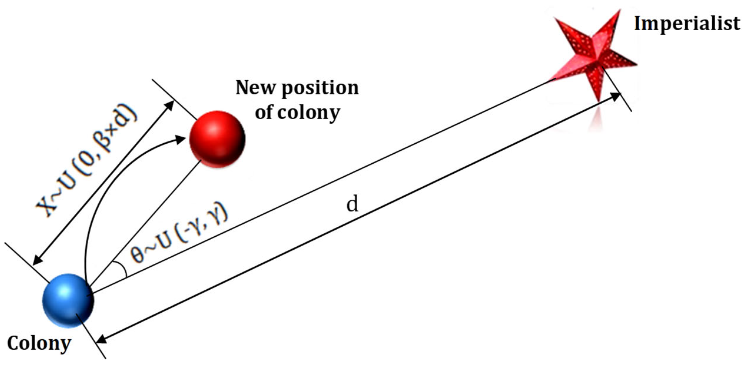
Following the formation of the initial empires, the colonies begin the assimilation phase by moving toward their respective imperialists (see Figure 5). This movement is precisely defined by two parameters: the displacement distance (X) and the deviation angle ($\theta$). X is calculated as a random variable drawn from a uniform distribution $U\left(0,\beta \times d\right)$ that generates a random number between 0 and $\beta \times d$, where d is the current distance between the colony and its imperialist, and $\beta$ is the assimilation coefficient (a value greater than 1). The $\theta$ is the deviation angle, which is also chosen as a random value from a uniform distribution $U\left(-\gamma ,\gamma \right)$, where $\gamma$ is an arbitrary angle that controls the maximum angular displacement (28; 34).

Step 3: Dual phase stochastic assimilation

The colonies within each empire undergo an assimilation phase. This phase enhances the population’s diversity and quality through genetic operations. Specifically, if the average colonies-imperialist distance value is above a certain threshold value dmax, the multi-points crossover operator takes place between colonies which improves solution’s convergence. Hence an exploitation phase will occur. Furthermore, if the average colonies-imperialist distance value drops below a certain threshold value dmin, the use of random replacement mutation operators serves to introduce entirely new colonies with potentially superior fitness (greater power), thereby improving the algorithm’s exploration capability and its chances of finding the global optimum [28,29].

Step 4: Exchange colony and imperialist positions

After the evolution step (which includes crossover and mutation) is completed, the cost functions of all colonies and imperialists are evaluated using Equation (2). Specifically, the cost functions calculated for the colonies’ new positions are compared against the cost function of their respective imperialist’s position. If any colony’s cost function is found to be less than that of its imperialist, meaning it represents a better FOPID parameter set, then a swap occurs: the successful colony takes the imperialist’s position, and the former imperialist reverts to being a colony.

Step 5: Generation of the Pareto front

This crucial step in the MOICA involves maintaining an archive (or external repository) that stores the non-dominated imperialists, which collectively represent the evolving Pareto front.

In the first iteration, N imperialists are initially selected. To populate the archive, the algorithm employs the fast-non-dominated sorting approach [28], where each imperialist’s objective function values (F1(DVs) = ISE and F2(DVs) = ITSE) are compared against all others [28,29]. The imperialists that are not dominated by any other solution (i.e., those that represent the best trade-offs) are then preserved in the archive to form the initial Pareto front.

For all subsequent iterations, the classification of the current imperialists is simplified: instead of comparing all imperialists against each other, their performance is evaluated solely through comparison with the solutions already contained within the previous Pareto front stored in the archive.

Step 6: Calculation of the total cost of empires

The total cost of an empire is a function of both the performance of its colonies and the performance (cost) of its own imperialist. Consequently, the total cost of the nth empire is formally defined as:

$$T{C}_n=Cos{t}_n+\xi mean\left(Cos{t}_{col,n}\right)$$

(16)

The parameter $\xi$ is a positive scaling factor constrained to the range between 0 and 1. The term $mean\left(Cos{t}_{col,n}\right)$ represents the average of the costs calculated for all the colonies belonging to that specific empire. The value chosen for $\xi$ directly controls the influence of the colonies on the empire’s total performance: a small value for $\xi$ results in a weak contribution from the colonies to the overall empire cost, while a large value for $\xi$ significantly increases the colonies’ influence.

Consequently, the normalized total cost of the nth empire is determined by the following expression:

$$NT{C}_n=\underset{i}{max}\left\{T{C}_i\right\}-T{C}_n$$

(17)

Step 7: Imperialistic competition

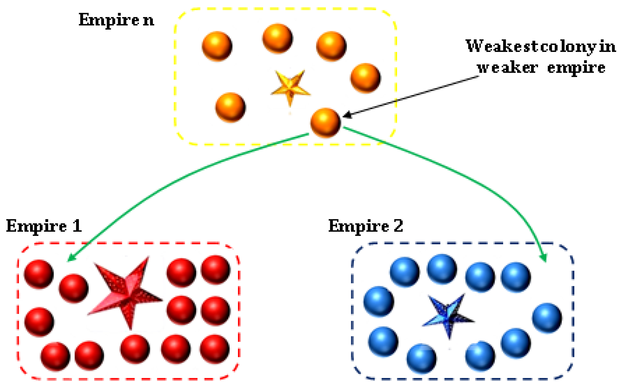
Once the total cost of each empire has been computed, the imperialistic competition phase commences. This competitive process, which models the struggle for power and resources among the empires, can be visualized as illustrated in Figure 6.

The most powerful empires acquire a portion of the weakest existing colonies. The number of colonies acquired is proportional to the empire’s calculated possession probability. This probability, which quantifies each empire’s likelihood of successfully capturing a colony during the competition phase, is determined by the following formula:

$$P_{p_n}=\left|{\displaystyle \frac{NT{C}_n}{{\sum }_{i}NT{C}_i}}\right|$$

(18)

The imperialistic competition is a continuous process designed to gradually facilitate the growth in power of the great empires while simultaneously causing a decline in the power of the weaker ones. Over time, these weaker empires steadily diminish in strength, and any empire that loses all its colonies collapses. The MOICA is designed to terminate when this competitive process naturally concludes, specifically when only one empire remains. This condition achieved only after all other, less powerful empires have collapsed.

5. Optimization Results and Performance Analysis

This section details the HTRS simulation carried out in MATLAB R2023a. The core of the control design involves applying the MOICA to optimize the FOPID performance. The overall structure of the HTRS model used for the simulation is illustrated in Figure 3. Simulation experiments are conducted under two distinct operating regimes:

Unload Running Condition: The system is excited by a step disturbance in the desired speed (speed setpoint).

Load Running Condition: The system is excited by a step disturbance in the load applied to the generator.

The specific parameters for the HTRS corresponding to these two running conditions are provided in

Table 2. Transfer Parameters for the Water Turbine and Generator under Two Operating Conditions.

Running Conditions		Unload Running Conditions	Load Running Conditions
Transmission coefficients in the water turbine and generator system	$e_x$	−1.0567	−1.2481
	$e_y$	0.908	1.313
	$e_h$	1.4191	1.3028
	$e_{qx}$	−0.0574	−0.1035
	$e_{qy}$	0.7887	1.0045
	$e_{qh}$	0.4571	0.3843
	$T_a$	12	8.5
	$e_g$	0.45	0.65

. The values for the remaining HTRS parameters are $T_w=1.5$ and $T_y=0.1$.

5.1. Optimization Setup and Reproducibility

During optimization, the hyperparameters presented in

Table 3. MOICA parameters.

Countries Number (Ncount)	Imperialists Number (Nimp)	Coefficient of Assimilation (β)	$\mathbf{Share} \mathbf{Coefficient} \left(\mathit{\xi }\right)$	Probability of Crossover (Pc)	Probability of Mutation (Pm)
1200	120	1.1	0.01	0.8	0.2

were selected to balance global exploration with local exploitation for the five-parameter FOPID tuning problem. These values were adopted based on the following justifications:

Population Size and Imperialists number: A robust population of 1200 was utilized to maintain genetic diversity across the complex objective space. According to [36], a population range of 500–2000 is optimal for 5-parameter optimization problems (like FOPID) to prevent premature convergence while maintaining computational efficiency. The ratio of 10% imperialists (120) follows the standard ICA framework, providing enough “power centers” to guide the search without clustering the population into a single local optimum too early [26].

Assimilation Coefficient: An assimilation coefficient of 1.1 ensures that colonies move toward their respective imperialists while maintaining a stable convergence rate. Values close to 1 are preferred in multi-objective scenarios to prevent the algorithm from overshooting the Pareto-optimal front [26,27].

Share Coefficient: This parameter controls the influence of the colonies on the total power of an empire. A small value of 0.01 ensures that the imperialist remains the primary driver of the search direction, while still allowing the colonies’ fitness to contribute to the empire’s competitive strength [27,28].

Crossover and Mutation Probabilities: To facilitate a high rate of information exchange between candidate solutions, the crossover and mutation probabilities were set at 0.8 and 0.2, respectively. These values were specifically selected to introduce sufficient stochasticity into the search process, thereby preventing the imperialist competition from stagnating within the complex, highly non-linear regions of the HTRS model [26,29,37].

The stability of the resulting Pareto front across multiple runs confirms that these settings provide a robust framework for identifying the optimal FOPID parameters.

The proposed framework has been executed using the following simulation Details:

• Discretization: All HTRS models and control loops are simulated in the MATLAB/Simulink R2023a environment using a fixed-step solver with a step size of 0.01 s.
• Performance Horizon: Each candidate controller is evaluated over a total simulation time of 20 s to ensure the complete capture of transient dynamics (overshoot and settling time).
• Constraint Handling: Constraints on the five FOPID parameters $[K_p,K_i, K_d$, λ, μ] are enforced through a “boundary-limited” approach. Any candidate solution generated outside the feasible ranges (specified in Table 1) is remapped to the nearest boundary value or assigned a high penalty cost.
• Termination Criteria: The optimization process terminates when only one empire remains after all other less powerful empires have collapsed.
• Reproducibility: To ensure consistent comparative results, the random number generator seed was fixed at a constant value for all optimization runs.

5.2. Multi-Objective Optimization Results for the HTRS in the Unloaded State

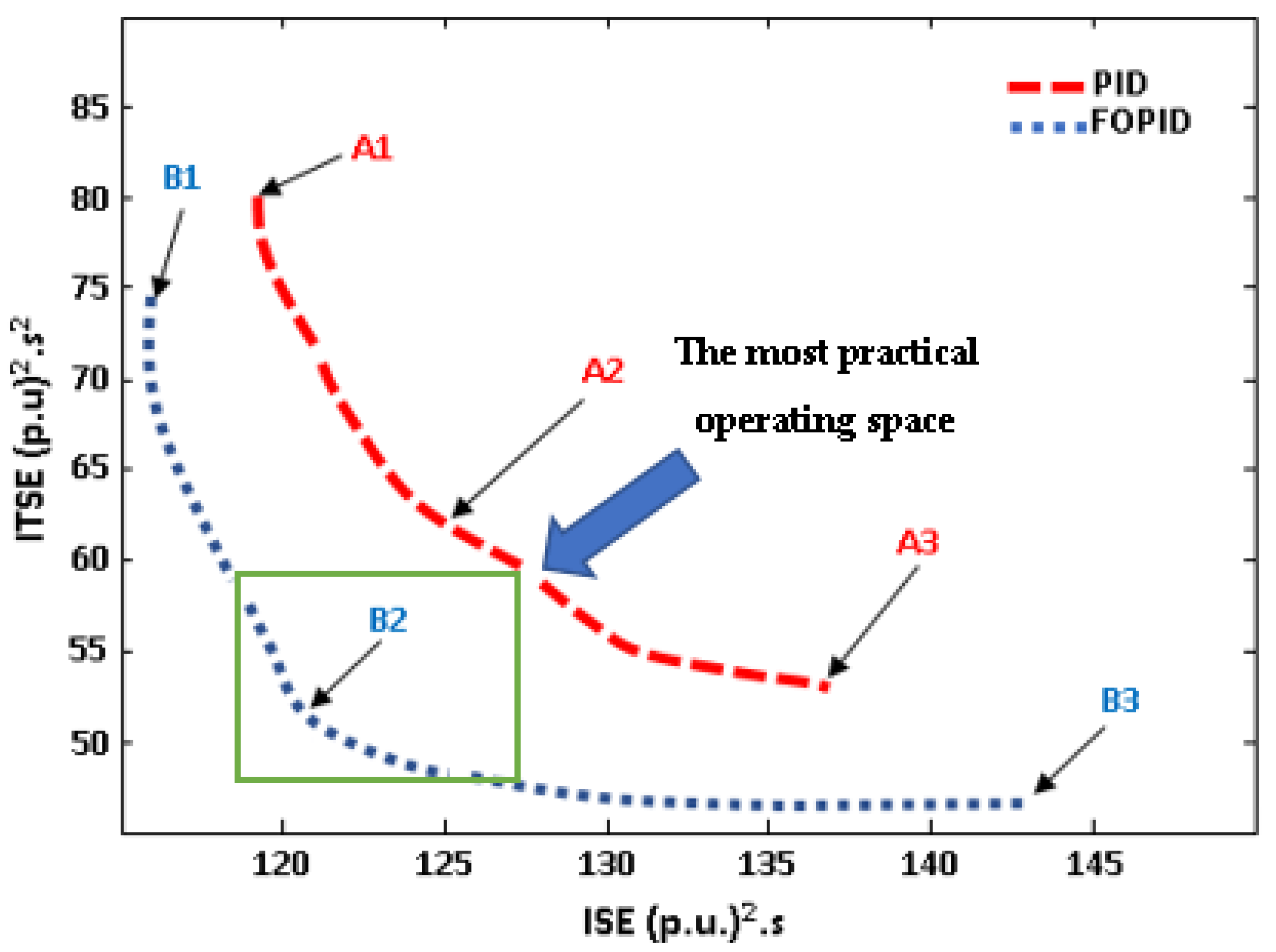
In this experimental phase, the proposed FOPID and traditional PID controllers are implemented within the HTRS. This allows for a direct comparison of their effectiveness in achieving superior dynamic performance. The system is tested under the unload running condition using a step perturbation in the desired speed (setpoint). The simulation is run over a 20 s time horizon. The resulting Pareto fronts, which illustrate the trade-off between the two contradictory objective functions, are displayed in Figure 7 for both the PID and FOPID controllers.

Figure 7 displays the Pareto fronts for both the FOPID and traditional PID controllers during the unload running condition. It illustrates the optimal trade-off solutions between the two conflicting objectives: ISE and ITSE. The most critical finding is the clear dominance of the FOPID Pareto front over the entire range of the PID Pareto front. Since the FOPID curve lies consistently below and to the left of the PID curve, it confirms that for any achievable level of ISE, the FOPID controller yields a lower ITSE. Conversely, for any ITSE, the FOPID achieves better ISE. This superior performance is a direct result of the FOPID’s extra degrees of freedom (λ and μ), allowing it to achieve a better simultaneous minimization of the two indices.

The inherent trade-off is evident in the slope of both fronts. Solutions moving toward the right, such as B3, prioritize minimizing ITSE to achieve faster settling times at the cost of higher ISE. Conversely, solutions moving toward the left, like B1, prioritize minimizing ISE for better tracking and lower overshoot, while accepting a longer settling time.

Quantitatively, the difference between the two controllers is significant. The FOPID controller achieves designs that are entirely non-dominated by even the best possible PID configuration. For instance, the best ISE solution for the PID (A1) is significantly outperformed by the FOPID solution (B1). This specific solution provides both a lower ISE and a lower ITSE. Ultimately, this highlights the FOPID’s ability to offer a broader and more effective range of optimal tuning points for the HTRS.

To select the most effective control configuration from the non-dominated Pareto front, the TOPSIS (Technique for Order of Preference by Similarity to Ideal Solution) method was employed. This technique ranks candidate solutions based on their geometric distance to an ideal reference point by using the closeness coefficient, calculated as follows [38]:

$$C_{c_j}={\displaystyle \frac{d_j^{-}}{{d_j^{+}+d}_j^{-}}}$$

(19)

where $d_j^{+}$ is the distance between the Pareto solution j and the best possible values for both objectives (ISEmin, ITSEmin). $d_j^{-}$ represents the distance between the Pareto solution j and the worst values observed on the front (ISEmax, ITSEmax).

By using TOPSIS method, B2 represents the optimal choice with a high closeness coefficient of 0.91. By achieving a closeness coefficient near unity, B2 is verified as the most balanced point on the curve, effectively defining a practically significant region of compromise that avoids the operational risks associated with extreme tuning. Specifically, the region around B2 solution defines the most practical operating space, as it avoids the extremes associated with either maximizing speed or maximizing accuracy. Crucially, the FOPID solution (B2) consistently dominates the PID solution (A2) within this compromise region. Because B2 sits below and to the left of A2, the FOPID mechanism simultaneously achieves a lower ITSE and a lower ISE. This outperformed the best possible balanced tuning achieved by the traditional PID controller. These results prove the superior trade-off capabilities of the fractional-order design within the HTRS.

Furthermore,

Table 4. Selected Solutions from the Pareto Front under Unload Running Conditions.

Controller		PID			FOPID
Selected Solution		A1	A2	A3	B1	B2	B3
F1(DVs) = ISE		119.94	125.28	136.47	116.12	121.33	143.18
F2(DVs) = ITSE		79.09	61.97	53.61	74.42	51.96	47.11
DVs	$K_p$	6.98	7.94	9.06	4.91	5.43	7.88
	$K_i$	0.44	0.55	0.57	0.68	0.75	0.98
	$K_d$	3.76	5.54	5.11	3.76	4.28	6.26
	λ	--	--	--	1.18	1.22	1.19
	μ	--	--	--	1.19	1.21	1.2

provides a detailed breakdown of several representative optimal solutions found along these Pareto fronts (Figure 8) for both control strategies.

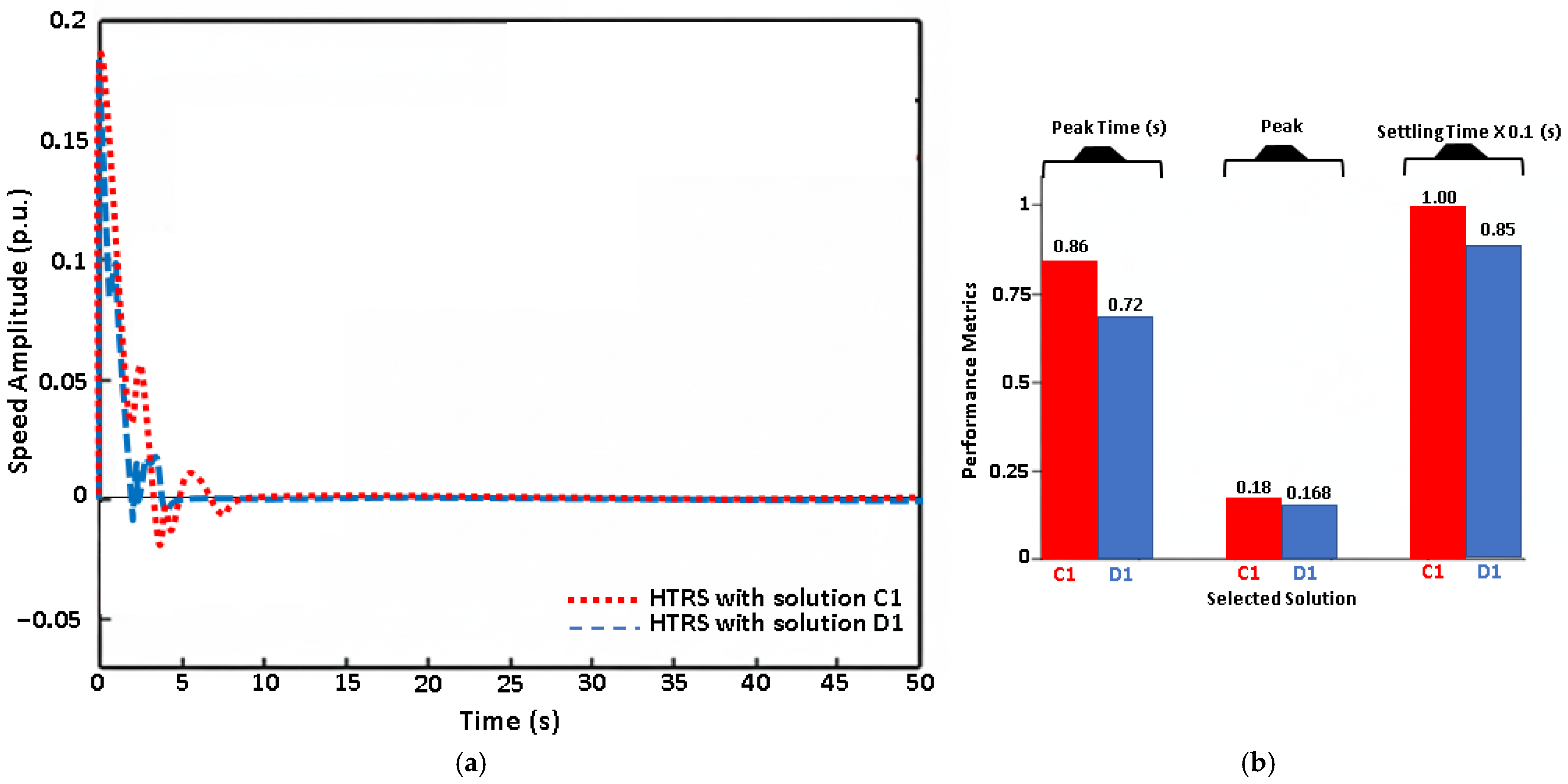
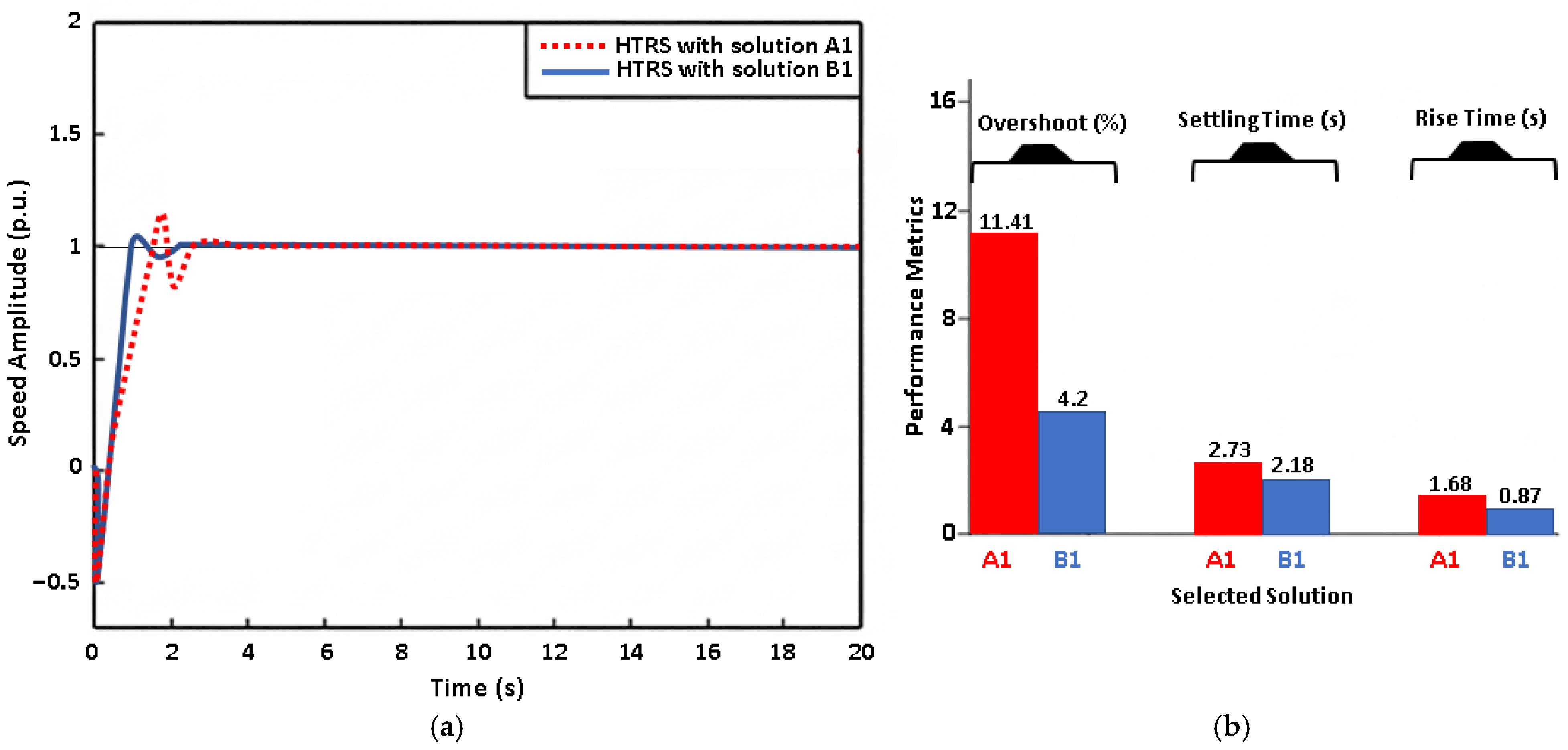
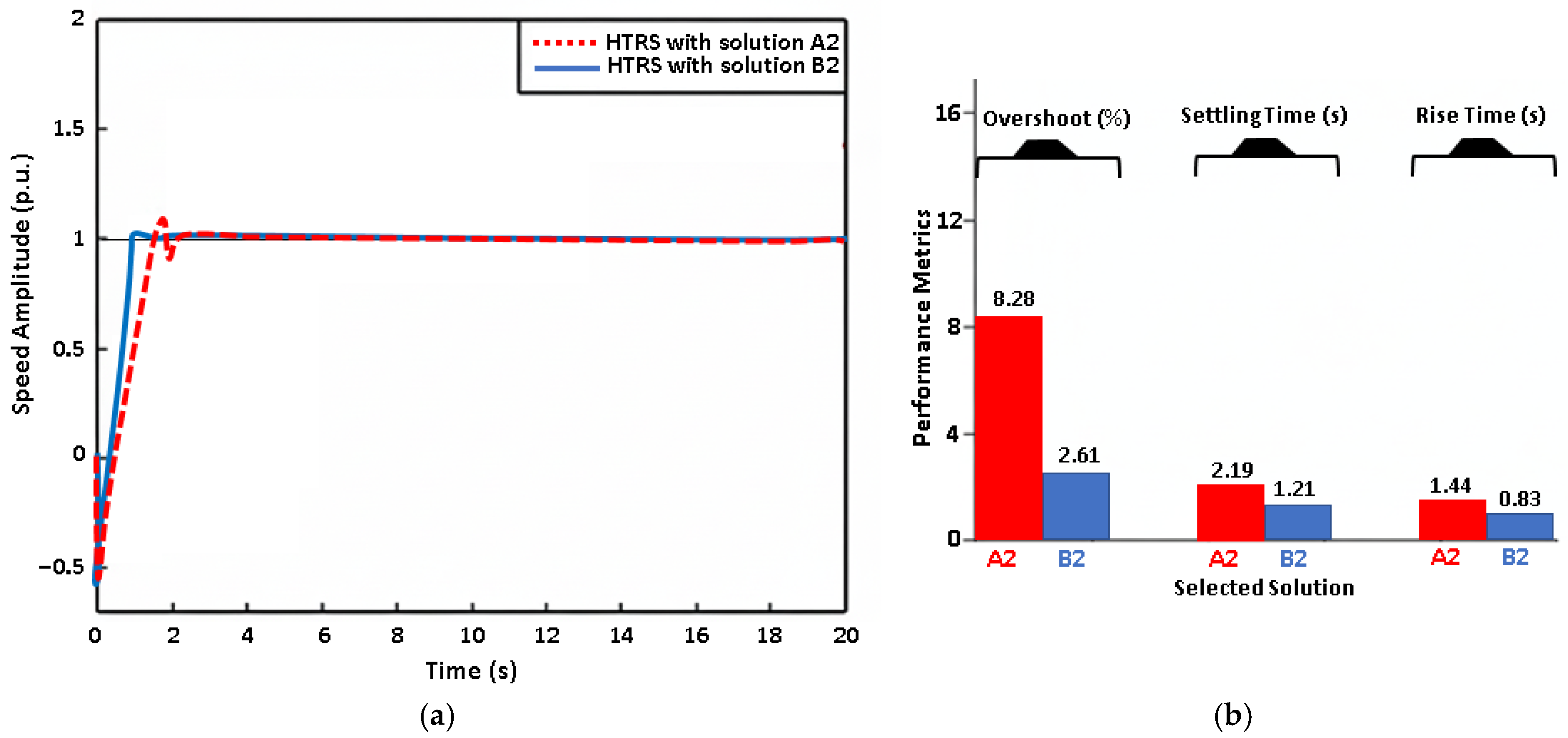
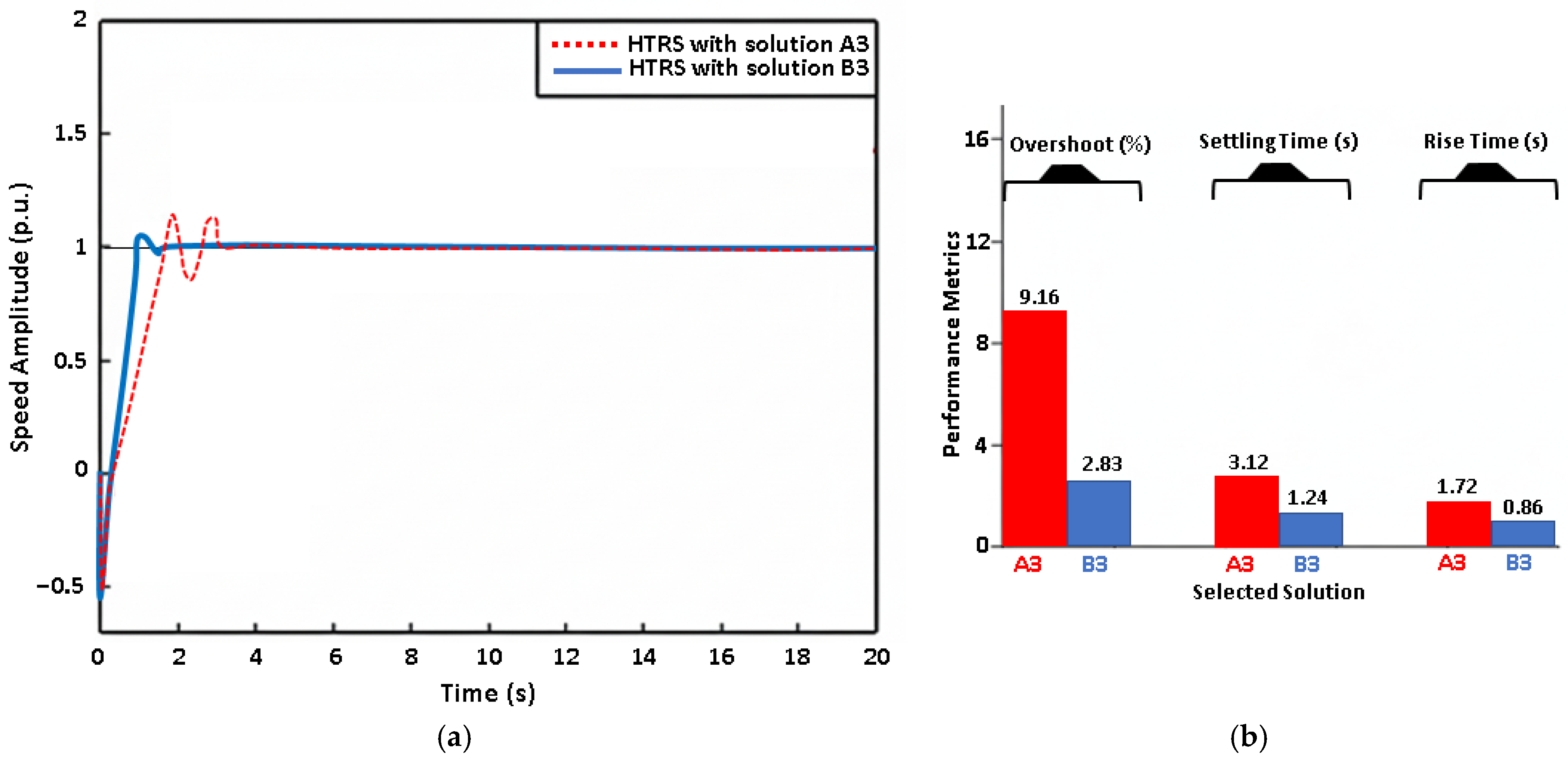
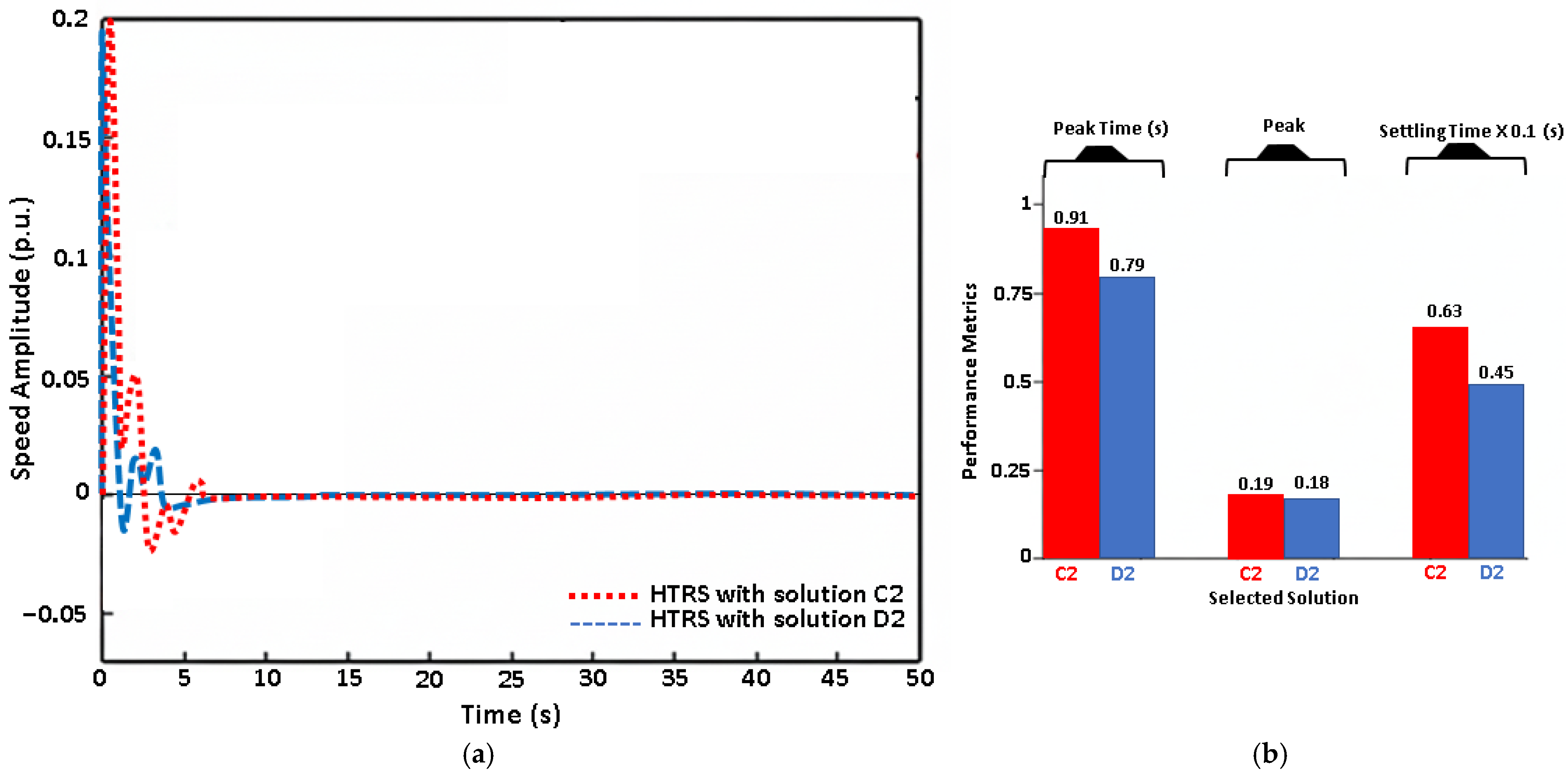
Figure 8, Figure 9 and Figure 10 display the setpoint tracking performance of the six representative control solutions (A1–A3, B1–B3), implemented with the corresponding controller parameters from Table 4.

Figure 8, Figure 9 and Figure 10 showing the setpoint tracking response for the representative solutions, detailed in Table 4, serve to validate the Pareto front results displayed in Figure 8. A key observation from these time-domain simulations is that the FOPID controller consistently delivers superior dynamic performance compared to the optimal traditional PID controller when applied to the HTRS. This superiority is confirmed across all obtained performance indicators such as rise time, settling time, and overshoot.

5.3. Multi-Objective Optimization Results for the HTRS in the Loaded State

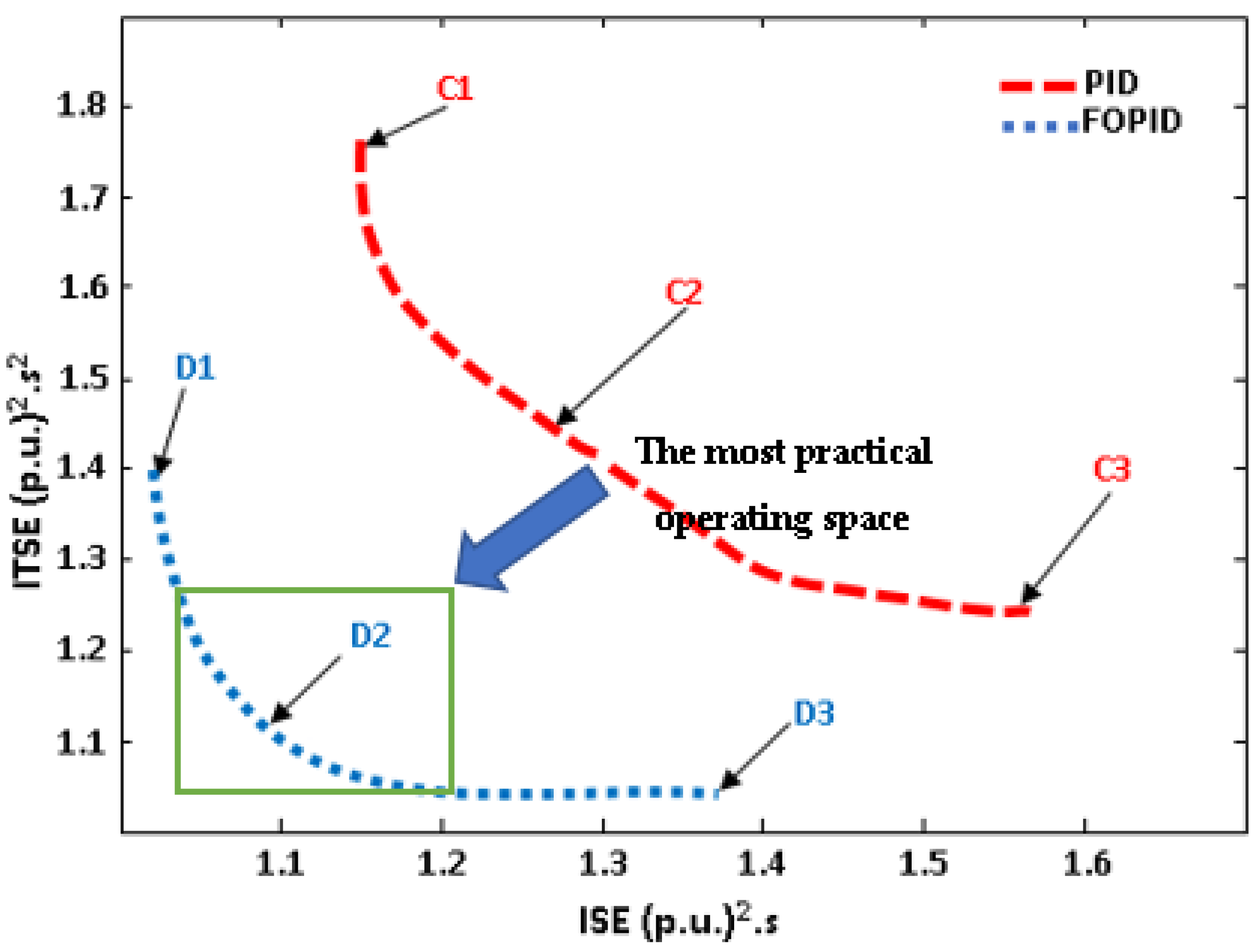
The optimal results obtained using the MOICA method are presented in Figure 11. This figure illustrates the Pareto fronts for both PID and FOPID controllers. It specifically compares their performance under a step load disturbance during load running. The results clearly demonstrate that the FOPID controller achieves significantly lower values of objective functions compared to the PID.

Figure 11 demonstrates the clear superiority of the FOPID controller, particularly within the area of best compromise between the two conflicting objectives: accuracy (ISE) and speed (ITSE). The FOPID front’s position, strictly below and to the left of the PID front, establishes its Pareto dominance. This conclusively demonstrates that the FOPID provides a superior solution for any performance point achievable by the PID controller. The FOPID simultaneously yields a faster response and higher accuracy. This is reflected in its ability to achieve both a lower ITSE and a lower ISE at the same time. This dominance highlights the FOPID’s ability to fundamentally expand the achievable performance boundary for load disturbance rejection in the HTRS.

By using TOPSIS method, D2 is selected as the optimal choice with a high closeness coefficient of 0.89. The most practical operating area lies near the middle section, specifically around D2. In this region, the curves begin to steepen significantly. This indicates a critical point where even a moderate reduction in ITSE results in a disproportionately large penalty in ISE. In this critical compromise zone, the performance gap between the two controllers is highly significant. This region is where control engineers typically select final parameters to achieve the best balance of speed and stability. Here, the FOPID offers solutions that yield a substantially lower ITSE for the same level of ISE compared to the PID.

Conversely, it can provide a much lower ISE for the same level of ITSE, outperforming the traditional PID in both metrics. This indicates that the FOPID mechanism provides a far more efficient trade-off for real-world applications. It superiorly balances the time required to settle after a load disturbance with the need to minimize the overall magnitude of the speed error.

In conclusion, the results unequivocally validate that the FOPID controller achieves a superior set of non-dominated tunings. This is made possible by the extra flexibility provided by the fractional-order differentiation and integration terms.

By examining the entire Pareto front, the data confirms that the FOPID controller is the optimal choice for the HTRS. It excels at the challenging task of ensuring effective and prompt load disturbance rejection.

Table 5. Selected Solutions from the Pareto Front under load Running Conditions.

Controller		PID			FOPID
Selected Solution		C1	C2	C3	D1	D2	D3
F1(DVs) = ISE		1.21	1.33	1.55	1.05	1.15	1.38
F2(DVs) = ITSE		1.79	1.45	1.25	1.42	1.1	1.06
DVs	$K_p$	6.73	6.88	7.06	10.98	10.04	10.16
	$K_i$	3.34	3.57	3.66	2.46	2.54	2.57
	$K_d$	3.76	3.86	3.83	2.74	3.14	3.16
	λ	--	--	--	1.22	1.18	1.16
	μ	--	--	--	1.28	1.26	1.22

lists representative solutions, selected from the extreme ends and the median, to characterize both the PID and FOPID Pareto fronts, thereby validating the findings of Figure 11.

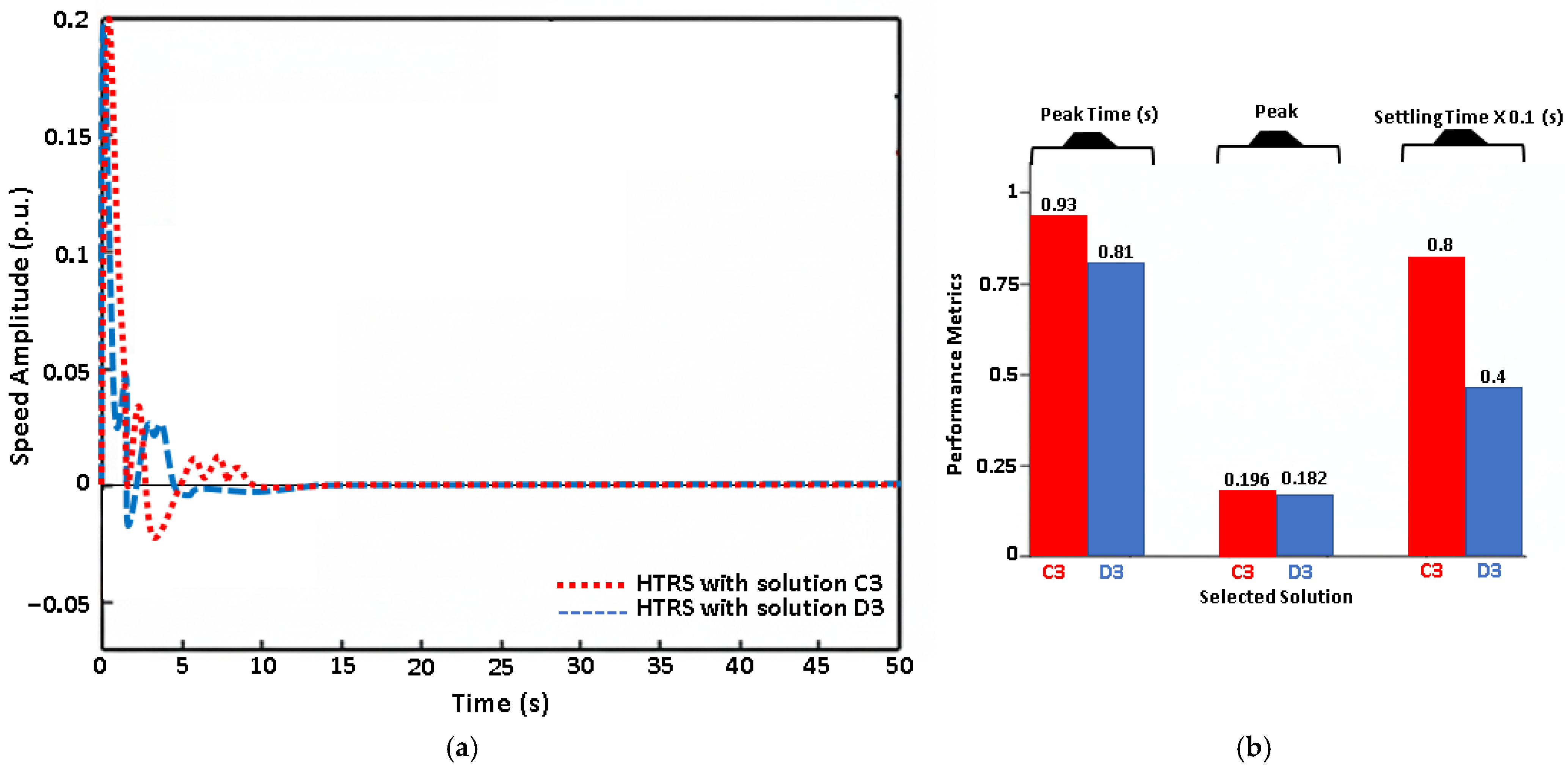
Figure 12, Figure 13 and Figure 14 illustrate the system’s transient response to a load disturbance for the six optimized representative solutions (C1–C3, D1–D3), using the controller parameters detailed in Table 5. To provide further detail, the performance metrics (peak time, peak deviation, and settling time) are explicitly noted on each figure for the corresponding time response. The FOPID controller demonstrates superior disturbance rejection speed by recovering rapidly from the unit load. In contrast, the PID controller exhibits a much slower recovery time when subjected to the same load disturbance.

The comparative analysis demonstrates that the FOPID controller consistently achieves a superior dynamic output for the HTRS, performing better than the conventional PID controller under both unloaded (setpoint tracking) and loaded (disturbance rejection) operating conditions. Given its effective handling of the inherent contradictory design objectives (e.g., maximizing speed while minimizing errors), the FOPID controller is the preferred and recommended solution within this multi-objective design framework.

6. Robustness and Validation: Comparative Analysis of Optimal Controller Solutions Under Parameter Uncertainty

6.1. Robustness of the Optimal Solutions Under Parameter Uncertainty

This robust analysis will investigate the effect of system parameter variations on the optimized controller solutions. The discussion will cover the two most common and critical operational scenarios encountered in the HTRS:

• Load Disturbance During Unload Running Condition (Setpoint Tracking Robustness): This tests the controller’s resilience when the primary operating state is setpoint tracking (unloaded), but a change in a system parameter occurs. The evaluation centers on Solution B2, which provides the most practical operating balance between speed (ITSE) and accuracy (ISE).
• Load Change During Load Running Condition (Disturbance Rejection Robustness): This examines the controller’s ability to maintain excellent disturbance rejection performance even when the system’s operational parameters shift simultaneously with the load event. Solution B2 is the focus of this evaluation because its parameters yield the most desirable compromise between the conflicting objectives.

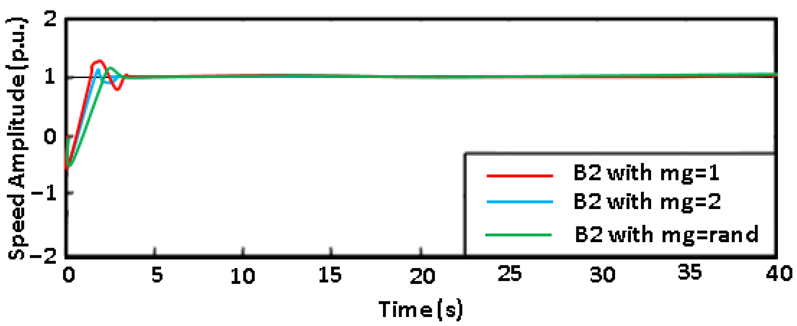
Figure 15 illustrates the robustness of the setpoint-tuned controllers. It shows their response to an unexpected load perturbation applied between 4 s and 10 s.

During this test, the system was operating under the nominal unloaded condition. This transient interval highlights how effectively each controller handles sudden changes.

The analysis assesses the sensitivity of FOPID design by comparing its dynamic time responses to various magnitudes of torque deviation (Under Unload condition).

The analysis presented in Figure 15 confirms the high robustness of the FOPID controller (Solution B2), which was meticulously determined using MOICA. This rigorous optimization process is crucial because it ensures the controller parameters are not only optimal for nominal conditions but also resilient to disturbances. The results graphically demonstrate this capability, showing that even when the load torque deviation magnitude is significantly varied, from the nominal (mg = 1) to the extreme (mg = 2) and the uncertain (mg = rand), the FOPID solution maintains stable and acceptable performance. Crucially, in all scenarios, the settling time remains fast and well under 5 s. This minimal sensitivity to parameter changes highlights how MOICA enables the FOPID design to effectively limit performance degradation. By maintaining stability under these conditions, the FOPID proves its inherent superiority and reliability over classical methods. It is better equipped to handle the real-world operational changes common in the HTRS.

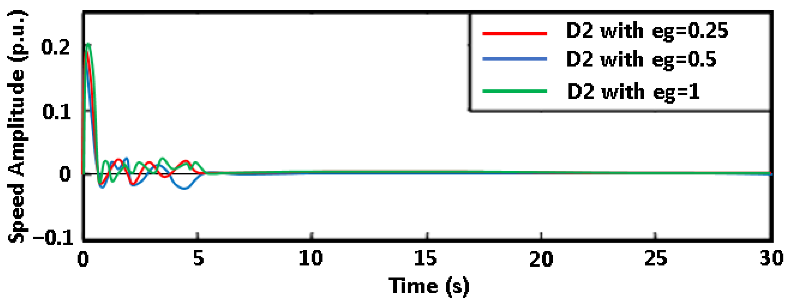
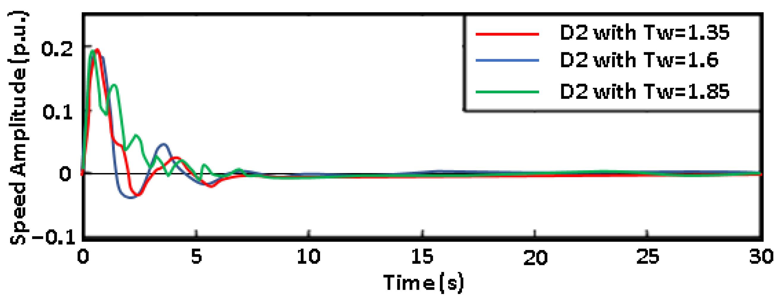
Figure 16 and Figure 17 illustrate the robustness of the controllers to variations in system parameters (eg and Tw), while the HTRS is operating under the loaded condition. This analysis is critical because frequent load changes typically cause the load self-regulation factor (eg) and the water starting time constant (Tw) to vary.

Figure 16 demonstrates the high robustness of the FOPID controller (Solution D2), which was meticulously tuned using the MOICA, to ensure resilience across varied operating conditions. This optimization process is critical because it yielded parameters that allow the controller to maintain satisfactory performance. The controller remains effective even when the load self-regulation factor (eg) is drastically varied from 0.25 to 1. This stability is particularly evident during load disturbance rejection. While the lowest (eg) provides the least natural system damping and slightly prolongs settling time, the FOPID solution consistently maintains stability. It quickly drives the speed deviation back to zero across all three test cases. This proves that the MOICA-derived FOPID design successfully compensates for significant parametric uncertainty in the load characteristics.

The results in Figure 17 demonstrate the high robustness of the FOPID controller (Solution D2). Specifically, the controller remains resilient against variations in the system’s inherent dynamics, such as the water starting time constant (Tw). The results show that the system maintains stability during load disturbance rejection, even as Tw varies significantly from 1.35 to 1.85. While a decrease in Tw causes slightly larger and faster initial oscillations, the controller remains effective. It quickly damps the speed deviation back to zero within approximately 8 s in all tested cases. This confirms that the MOICA-derived design successfully compensates for the natural parameter uncertainty of the system.

While physical HTRS installations may encounter secondary non-idealities such as measurement noise and actuator saturation, the robustness tests conducted here focus on mg, eg, and Tw because they represent the primary physical sensitivities of the hydraulic-mechanical coupling. Mathematically, the FOPID controller’s fractional derivative (μ) provides a more flexible frequency response than integer-order controllers, offering a degree of natural immunity to high-frequency noise. Furthermore, by optimizing the controller using the ITSE criterion, which applies a time-weighted penalty to transient errors, the resulting parameters inherently prioritize high phase margins. This ensures that the system remains stable even in the presence of unmodeled dynamics such as sensor delays or minor parametric drifts, fulfilling the requirements for a realistic and reliable regulation performance.

6.2. Comparison of Optimal Solutions with Literature

This section provides a comparative analysis to validate the superiority of the FOPID controller tuned using the MOICA against relevant state-of-the-art results from the literature. We compare the optimal Pareto front solutions, which were optimized for the conflicting objectives of minimizing ISE and ITSE. These results are measured against FOPID controllers tuned using other common multi-objective algorithms. Specifically, the comparison includes the Genetic Algorithm (GA), Multi-Objective Particle Swarm Optimization (MOPSO), and Multi-objective Harris Hawks (MOHHO). This comparison is carried out under two critical operating scenarios for the HTRS: unloaded conditions and loaded conditions.

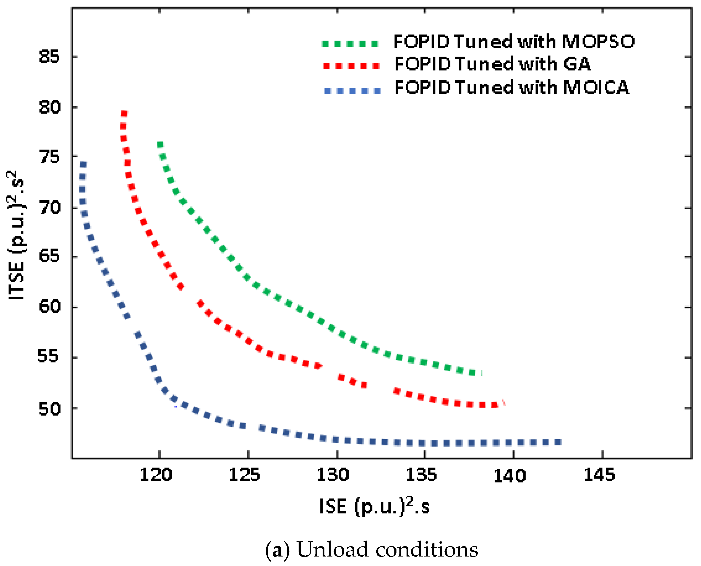
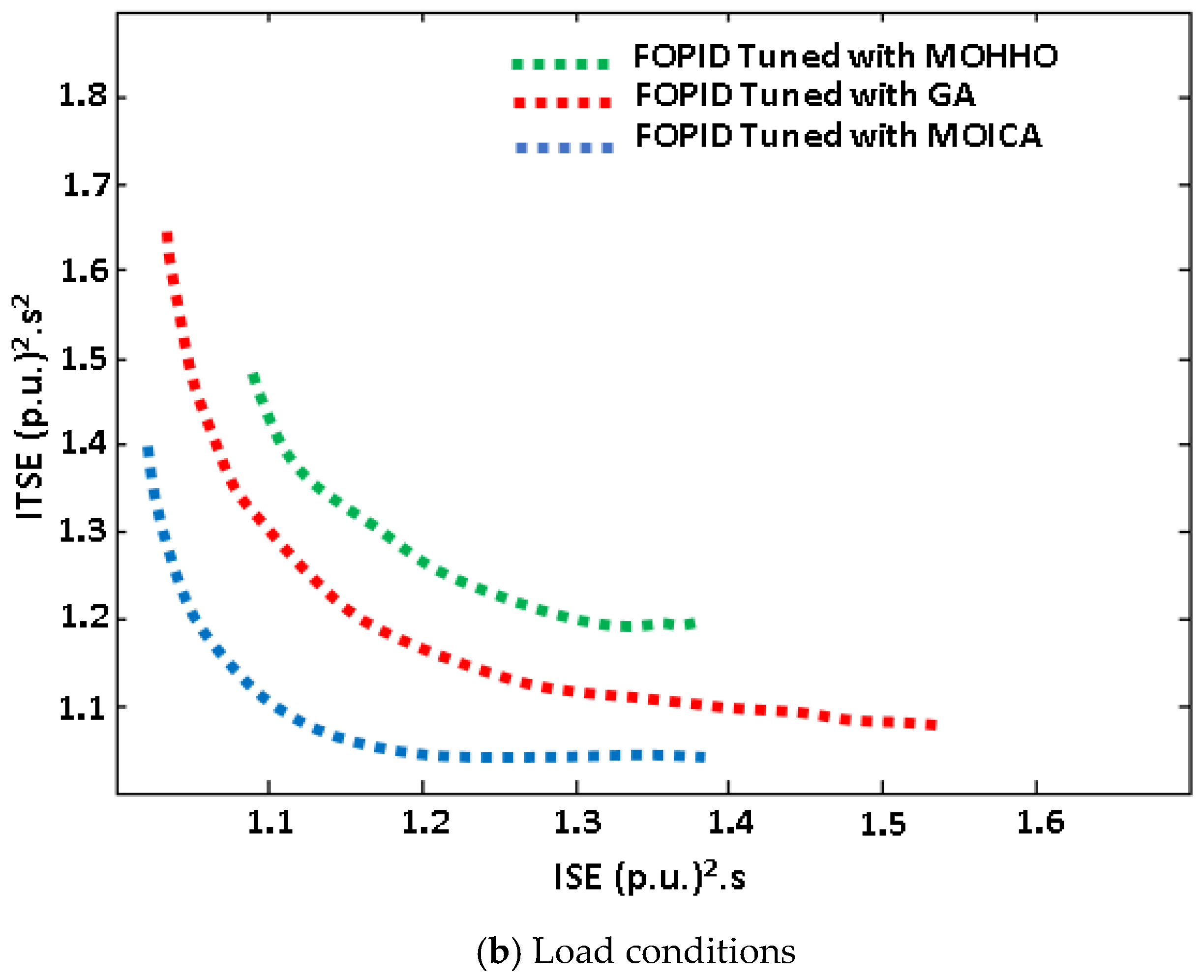
The Pareto fronts (Figure 18) demonstrate the superior optimization capability of the MOICA for tuning the FOPID controller. This superiority translates into quantifiable performance improvements over the literature benchmarks (GA [21], MOPSO [19], and MOHHO [22]).

6.2.1. Unload Conditions

Figure 18a confirms that the FOPID controller tuned with MOICA achieves Pareto dominance over both GA and MOPSO. This means the MOICA-tuned controller can simultaneously provide a lower ISE and a lower ITSE. For more details, the following table presents comparison of MOICA, GA, and MOPSO for FOPID tuning.

According to Figure 18a and

Table 6. Comparing MOICA, GA, and MOPSO for FOPID tuning.

Comparison Point	MOICA	GA	Improvement % of MOICA vs. GA	MOPSO	Improvement % of MOICA vs. MOPSO
ISE values at ITSE = 50	126	136	7.3%	N/A	N/A
ITSE values at ISE = 130	42	52	19.23%	57	26.32%
ITSE values at ISE = 120	50	61	18.03%	68	26.47%

N/A: Not Available.

, one can note that the MOICA for FOPID tuning provides:

Speed Maximization: For a moderate level of accuracy (e.g., at ISE = 130), the MOICA solution achieves a 19% to 26% lower ITSE (faster response and settling time) compared to GA and MOPSO, respectively. This substantial improvement is crucial for maximizing efficiency during minimal load operation where fast speed changes are required.

Accuracy Maximization: For the lowest achievable ITSE, the MOICA-tuned controller still offers higher accuracy. At ITSE = 50, the MOICA solution is approximately 7.3% more accurate (lower ISE) than the corresponding GA solution.

6.2.2. Load Conditions

Figure 18b shows that the FOPID tuned with MOICA also maintains strict Pareto dominance against GA and MOHHO, demonstrating superior robustness and recovery from system disturbances.

Based on Figure 18b and

Table 7. Comparing MOICA, GA, and MOHHO for FOPID tuning.

Comparison Point	MOICA	GA	Improvement % of MOICA vs. GA	MOHHO	Improvement % of MOICA vs. MOHHO
ISE values at ITSE = 1.2	1.07	1.17	8.55%	1.32	18.94%
ITSE values at ISE = 1.35	1.05	1.14	7.89%	1.24	15.32%
ITSE values at ISE = 1.1	1.11	1.32	15.91%	1.46	23.97%

, the MOICA approach for FOPID tuning yields:

Robustness (ITSE/ISE Balance): For a given accuracy level (e.g., at ISE = 1.1), the MOICA solution is significantly faster, achieving a 15.9% to 23.9% lower ITSE than GA and MOHHO, respectively. This means the MOICA-tuned HTRS recovers stability far more quickly after a load disturbance.

Accuracy (ISE) Under Stress: For a given recovery speed (e.g., at ITSE = 1.2), the MOICA solution is 8.55% to18.94% more accurate (lower ISE) than the GA and MOHHO solutions, demonstrating superior disturbance rejection magnitude.

The use of the MOICA unequivocally validates its status as the optimal optimization technique for this application. The consistent Pareto dominance in both scenarios (Unload and load conditions) is backed by quantitative evidence, showing that MOICA provides improvements in performance metrics:

Setpoint Tracking (Unload): Up to 26% improvement in settling speed (ITSE) and about 8% improvement in ISE.

Disturbance Rejection (Load): Up to 23% improvement in recovery speed (ITSE) and 18.9% improvement in error suppression magnitude (ISE).

This superior capacity to manage the trade-off between speed (ITSE) and accuracy (ISE) results in a more advanced FOPID controller. Compared to literature benchmarks, the MOICA’s final design is both superior and more robust. These characteristics make it the most practical choice for real-world implementation in the HTRS.

6.2.3. Comparative Discussion: FOPID + MOICA vs. Fuzzy Logic Control

While the proposed FOPID controller demonstrates high performance, Fuzzy Logic Controllers (FLC) are also frequently employed for the frequency regulation of synchronous generators and hydraulic turbines [30]. FLCs excel in managing system uncertainties and non-linearities by utilizing linguistic “if-then” rules rather than rigid analytical models. However, the effectiveness of the proposed FOPID + MOICA framework compared to traditional FLC approaches is summarized in

Table 8. Qualitative performance comparison: FOPID + MOICA vs. Fuzzy Logic Control.

Feature	Proposed FOPID + MOICA	Fuzzy Logic Controller (FLC)
Design Methodology	Analytical/Fractional Calculus	Heuristic/Linguistic Rules
Tuning Mechanism	Automated Global Optimization (MOICA)	Often manual or expert-driven tuning
Multi-Objective Capability	Generates a Pareto-optimal front	Difficult to achieve without hybrid structures
Mathematical Precision	High (exact coefficients $K_p,K_i, K_d$, λ and μ)	Qualitative (membership functions)
Computational Burden	Low (direct linear/fractional implementation)	High (requires real-time fuzzy inference)

. The primary advantage of the MOICA-tuned FOPID lies in its ability to provide a systematic, multi-objective trade-off between transient metrics (ISE and ITSE). Unlike FLCs, which often require subjective expert knowledge for rule-base design and membership function tuning, the MOICA approach is purely data-driven and ensures that the controller parameters are globally optimal within the defined search space.

Furthermore, while hybrid systems such as PSO-Fuzzy PID [30] have been developed to improve FLC performance, the fractional-order nature of the proposed controller inherently provides two additional degrees of freedom, allowing for a more flexible and precise response than standard integer-order fuzzy-hybrid variants.

7. Conclusions

This study addressed the inherent complexity of tuning the five parameters of the Fractional Order Proportional-Integral-Derivative (FOPID) controller for the Hydraulic Turbine Regulating System (HTRS), by utilizing the Multi-Objective Imperialist Competitive Algorithm (MOICA). The controller design was strategically framed as a multi-objective optimization problem.

This approach focused on generating a comprehensive Pareto front by simultaneously minimizing two contradictory transient performance metrics. Specifically, the design optimizes both the Integral of Squared Error (ISE) and the Integral of Time Multiplied Squared Error (ITSE). This methodology provides practical engineers with a range of optimal solutions, allowing them to select the controller that best balances accuracy and speed for specific operational requirements.

The simulation results unequivocally established the superiority of the MOICA-tuned FOPID controller across the full operational spectrum. The FOPID demonstrated significantly better dynamic performance, including faster settling time and lower peak deviation, compared to the conventional integer-order PID controller under both unloaded (setpoint tracking) and loaded (disturbance rejection) conditions. Furthermore, the MOICA solutions were proven to dominate FOPID controllers tuned using alternative multi-objective algorithms from the literature (such as GA, MOHHO, and MOPSO) across all performance metrics. Critically, the MOICA-FOPID delivered superior dynamic performance, achieving up to a 26% improvement in settling speed (ITSE) and about an 8% improvement in accuracy (ISE) during Setpoint Tracking (Unload conditions). Its dominance was even more pronounced under Disturbance Rejection (Load conditions), where it showed up to a 23% improvement in recovery speed (ITSE) and a substantial 18.9% improvement in error suppression magnitude (ISE) compared to the alternative optimization techniques. The superior capacity to manage the trade-off between speed (ITSE) and accuracy (ISE) results in a highly effective FOPID controller.

This final design is both superior and more robust than current literature benchmarks. Consequently, it stands as the most practical choice for real-world implementation in the HTRS. Critically, the final optimal FOPID design exhibited high robustness. It effectively maintained stable and acceptable transient performance even during significant variations in key parameters. Specifically, the design remained resilient against changes in load torque deviation (mg), the load self-regulation factor (eg) and the water starting time constant (Tw).

Building upon the successful validation of the MOICA-FOPID design, future research should explore several avenues to further enhance the system’s performance and practical applicability. Potential future work includes implementing the optimized FOPID controller on a real-time HTRS experimental platform to validate its performance under actual physical constraints and noise. Additionally, exploring the use of adaptive or self-tuning FOPID strategies could ensure the controller can automatically adjust its parameters in real-time to sudden and prolonged changes in operating conditions or severe system degradation.

References

1. Wang, C.; Wang, D.-K.; Zhang, J.-M. Experimental Study on the Optimal Strategy for Power Regulation of Governing System of Hydropower Station. Water 2021, 13, 421. [Google Scholar] [CrossRef]
2. Ghamari, S.M.; Habibi, D.; Aziz, A. Robust Adaptive Fractional-Order PID Controller Design for High-Power DC-DC Dual Active Bridge Converter Enhanced Using Multi-Agent Deep Deterministic Policy Gradient Algorithm for Electric Vehicles. Energies 2025, 18, 3046. [Google Scholar] [CrossRef]
3. El-Sousy, F.F.M.; Aly, M.; Alqahtani, M.H.; Aljumah, A.S.; Almutairi, S.Z.; Mohamed, E.A. New Cascaded 1+PII2D/FOPID Load Frequency Controller for Modern Power Grids including Superconducting Magnetic Energy Storage and Renewable Energy. Fractal Fract. 2023, 7, 672. [Google Scholar] [CrossRef]
4. Maghami, M.R.; Mutambara, A.G.O. Challenges associated with Hybrid Energy Systems: An artificial intelligence solution. Energy Rep. 2023, 9, 924–940. [Google Scholar] [CrossRef]
5. Wendimu, A.A.; Matušů, R.; Shaikh, I. Fractional-order PID control for elevation and azimuth in a twin rotor system. Sci. Rep. 2025, 15, 33590. [Google Scholar] [CrossRef] [PubMed]
6. Rameshar, V.; Sharma, G.; Bokoro, P.N.; Çelik, E. Frequency Support Studies of a Diesel–Wind Generation System Using Snake Optimizer-Oriented PID with UC and RFB. Energies 2023, 16, 3417. [Google Scholar] [CrossRef]
7. Kez, D.A.; Foley, A.M.; Ahmed, F.; Morrow, D.J. Overview of frequency control techniques in power systems with high inverter-based resources: Challenges and mitigation measures. IET Smart Grid 2023, 6, 341–362. [Google Scholar] [CrossRef]
8. Singh, B.; Slowik, A.; Bishnoi, S.K. Review on Soft Computing-Based Controllers for Frequency Regulation of Diverse Traditional, Hybrid, and Future Power Systems. Energies 2023, 16, 1917. [Google Scholar] [CrossRef]
9. Haro-Larrode, M.; Gomez-Jarreta, A. Design Guidelines for Fractional Order Cascade Control in DC Motors: A Computational Analysis on Pairing Speed and Current Loop Orders Using Oustaloup’s Recursive Method. Machines 2025, 13, 61. [Google Scholar] [CrossRef]
10. Chuong, V.L.; Nam, N.H.; Giang, L.H.; Vu, T.N.L. Robust Fractional-Order PI/PD Controllers for a Cascade Control Structure of Servo Systems. Fractal Fract. 2024, 8, 244. [Google Scholar] [CrossRef]
11. Frikh, M.L.; Boutasseta, N. Pitch Angle Control of Wind Turbines Using Model-Free Auto-Tuned Fractional Order Proportional Derivative ATFOPD Controller. Comput. Electr. Eng. 2024, 116, 109199. [Google Scholar] [CrossRef]
12. Guedida, S.; Tabbache, B.; Benzaoui, K.M.S.; Nounou, K.; Nesri, M. Novel Speed Sensorless DTC Design for a Five-Phase Induction Motor with an Intelligent Fractional Order Controller Based-MRAS Estimator. Power Electron. Drives 2024, 9, 63–85. [Google Scholar] [CrossRef]
13. Almutairi, S.; Anayi, F.; Packianather, M.; Shouran, M. An Optimal Two-Stage Tuned PIDF + Fuzzy Controller for Enhanced LFC in Hybrid Power Systems. Sustainability 2025, 17, 9109. [Google Scholar] [CrossRef]
14. El-Rifaie, A.M.; Abid, S.; Ginidi, A.R.; Shaheen, A.M. Fractional Order PID Controller Based-Neural Network Algorithm for LFC in Multi-Area Power Systems. Eng. Rep. 2025, 7, e12866. [Google Scholar] [CrossRef]
15. Tuan, D.H.; Thanh, V.N.N.; Chi, D.N.; Pham, V.H. Improving Frequency Control of Multi-Area Interconnected Hydro-Thermal Power System Using PSO Algorithm. Appl. Sci. 2025, 15, 2898. [Google Scholar] [CrossRef]
16. Micev, M.; Ćalasan, M.; Oliva, D. Fractional Order PID Controller Design for an AVR System Using Chaotic Yellow Saddle Goatfish Algorithm. Mathematics 2020, 8, 1182. [Google Scholar] [CrossRef]
17. Kurokawa, R.; Sato, T.; Vilanova, R.; Konishi, Y. Discrete-Time First-Order Plus Dead-Time Model-Reference Trade-off PID Control Design. Appl. Sci. 2019, 9, 3220. [Google Scholar] [CrossRef]
18. Zhu, M.; Xu, Z.; Zang, Z.; Dong, X. Design of FOPID Controller for Pneumatic Control Valve Based on Improved BBO Algorithm. Sensors 2022, 22, 6706. [Google Scholar] [CrossRef]
19. Zhang, N.; Li, C.; Lai, X. Design of a Multi-Conditions Adaptive Fractional Order PID Controller for Pumped Turbine Governing System using Multiple Objectives Particle Swarm Optimization. In Proceedings of the 4th International Conference on Electromechanical Control Technology and Transportation (ICECTT 2019), Guilin, China, 26–28 April 2019; pp. 39–44. [Google Scholar]
20. Makhbouche, A.; Boudjehem, B.; Birs, I.; Muresan, C.I. Fractional-Order PID Controller Based on Immune Feedback Mechanism for Time-Delay Systems. Fractal Fract. 2023, 7, 53. [Google Scholar] [CrossRef]
21. Chen, Z.H.; Yuan, X.H.; Ji, B.; Wang, P.T.; Tian, H. Design of a fractional order PID controller for hydraulic turbine regulating system using chaotic non-dominated sorting genetic algorithm II. Energy Convers. Manag. 2014, 84, 390–404. [Google Scholar] [CrossRef]
22. Fu, W.; Lu, Q. Multiobjective optimal control of FOPID controller for hydraulic turbine governing systems based on reinforced multiobjective Harris Hawks optimization coupling with hybrid strategies. Complexity 2020, 2020, 8885141. [Google Scholar] [CrossRef]
23. Dai, F.; Ma, T.; Gao, S. Optimal Design of a Fractional Order PIDD$^2$ Controller for an AVR System Using Hybrid Black-Winged Kite Algorithm. Electronics 2025, 14, 2315. [Google Scholar] [CrossRef]
24. Altbawi, S.M.A.; Mokhtar, A.S.B.; Jumani, T.A.; Khan, I.; Hamadneh, N.N.; Khan, A. Optimal design of Fractional order PID controller based Automatic voltage regulator system using gradient-based optimization algorithm. J. King Saud Univ.-Eng. Sci. 2024, 36, 32–44. [Google Scholar] [CrossRef]
25. Liu, S.; Lin, Z.; Feng, R.; Huang, W.; Yan, B. Intelligent control method for automatic voltage regulator: An improved coati optimization algorithm-based strategy. Measurement 2025, 252, 117263. [Google Scholar] [CrossRef]
26. Najlaoui, B.; Alghafis, A.; Nejlaoui, M. Robust design of a low-cost flat plate collector under uncertain design parameters. Energy Rep. 2023, 10, 2950–2961. [Google Scholar] [CrossRef]
27. Nejlaoui, M.; Alghafis, A.; Sadig, H. Six sigma robust multi-objective design optimization of flat plate collector system under uncertain design parameters. Energy 2022, 239, 121883. [Google Scholar] [CrossRef]
28. Nejlaoui, M.; Najlawi, B.; Alsagri, A.S. A multi-objective methodology for multi-criteria engineering design. Appl. Soft Comput. 2020, 91, 106204. [Google Scholar] [CrossRef]
29. Najlaoui, B.; Alghafis, A.; Sadig, H.; Raouf, E.A.; Hassen, M.A. Multi-Objective Design Optimization and Experimental Investigation of a Low-Cost Solar Desalination System Under Al Qassim Climate. Sustainability 2025, 17, 1771. [Google Scholar] [CrossRef]
30. Elhawat, M.; Altınkaya, H. Frequency Regulation of Stand-Alone Synchronous Generator via Induction Motor Speed Control Using a PSO-Fuzzy PID Controller. Appl. Sci. 2025, 15, 3634. [Google Scholar] [CrossRef]
31. Guo, W.; Zhu, D. A Review of the Transient Process and Control for a Hydropower Station with a Super Long Headrace Tunnel. Energies 2018, 11, 2994. [Google Scholar] [CrossRef]
32. Zhang, J.; Liu, S.; Li, J.; Li, D.; Wang, Z. An Improved ADRC Design Based on a Generalized Differentiator for a Nonlinear Hydraulic Turbine Regulating System. Processes 2025, 13, 86. [Google Scholar] [CrossRef]
33. Wang, L.; Zhang, K.; Zhao, W. Nonlinear Modeling of Dynamic Characteristics of Pump-Turbine. Energies 2022, 15, 297. [Google Scholar] [CrossRef]
34. Zhang, N.; Li, C.; Ni, Z.; Mao, Y. A mixed-strategy based gravitational search algorithm for parameter identification of hydraulic turbine governing system. Knowl.-Based Syst. 2016, 109, 218–227. [Google Scholar] [CrossRef]
35. Kishor, N.; Singh, S.P.; Raghuvanshi, A.S. Dynamic simulations of hydro turbine and its state estimation based LQ control. Energy Convers. Manag. 2006, 47, 3119–3137. [Google Scholar] [CrossRef]
36. Atashpaz-Gargari, E.; Lucas, C. Imperialist competitive algorithm: An algorithm for optimization inspired by imperialistic competition. In Proceedings of the 2007 IEEE Congress on Evolutionary Computation (CEC), Singapore, 25–28 September 2007; pp. 4661–4667. [Google Scholar] [CrossRef]
37. Daraz, A.; Malik, S.A.; Basit, A.; Aslam, S.; Zhang, G. Modified FOPID Controller for Frequency Regulation of a Hybrid Interconnected System of Conventional and Renewable Energy Sources. Fractal Fract. 2023, 7, 89. [Google Scholar] [CrossRef]
38. Kamalizadeh, S.; Niknam, S.A.; Balazinski, M.; Turenne, S. The Use of TOPSIS Method for Multi-Objective Optimization in Milling Ti-MMC. Metals 2022, 12, 1796. [Google Scholar] [CrossRef]
Figure 1. Hydraulic turbine regulating system structure. Legend: Dashed lines (governor control signals); color-coded wiring (three-phase transmission); and red triangle symbols (reservoir water levels).
Fractalfract 10 00046 g001
Figure 2. General layout of HTRS.
Fractalfract 10 00046 g002
Figure 3. The closed-loop configuration of the HTRS utilizing the FOPID controller.
Fractalfract 10 00046 g003
Figure 4. Pseudocode of MOICA for FOPID Tuning.
Fractalfract 10 00046 g004
Figure 5. Shifting colonies toward their imperial leaders.
Fractalfract 10 00046 g005
Figure 6. Competition among empires. Legend: Star Symbols (imperialists); colored Spheres (colonies); dashed rectangles (empires boundaries) and solid arrows (absorption process).
Fractalfract 10 00046 g006
Figure 7. The Pareto front for the PID and FOPID controllers during unload running. Legend: Black arrows denote selected optimal solutions; blue arrow indicates the most practical solution space; circles/squares differentiate between PID and FOPID data points.
Fractalfract 10 00046 g007
Figure 8. Step response comparison for representative solutions A1 and B1. (a) Speed amplitude, (b) performance metric.
Fractalfract 10 00046 g008
Figure 9. Step response comparison for representative solutions A2 and B2. (a) Speed amplitude, (b) performance metric.
Fractalfract 10 00046 g009
Figure 10. Step response comparison for representative solutions A3 and B3. (a) Speed amplitude, (b) performance metric.
Fractalfract 10 00046 g010
Figure 11. PID and FOPID optimal results during Loaded running. Legend: Black arrows denote selected optimal solutions; blue arrow indicates the most practical solution space; circles/squares differentiate between PID and FOPID data points.
Fractalfract 10 00046 g011
Figure 12. Load disturbance rejection performance comparison for representative solutions C1 and D1; (a) speed amplitude, (b) performance metric.
Fractalfract 10 00046 g012
Figure 13. Load disturbance rejection performance comparison for representative solutions C2 and D2; (a) speed amplitude, (b) performance metric.
Fractalfract 10 00046 g013
Figure 14. Load disturbance rejection performance comparison for representative solutions C3 and D3; (a) speed amplitude, (b) performance metric.
Fractalfract 10 00046 g014
Figure 15. Robustness of FOPID designs various magnitudes of load torque deviation (Unload running condition).
Fractalfract 10 00046 g015
Figure 16. Robustness of FOPID designs various load self-regulation factors (load running condition).
Fractalfract 10 00046 g016
Figure 17. Robustness of FOPID design various water starting time constant (load running condition).
Fractalfract 10 00046 g017
Figure 18. Comparison of FOPID tuned with MOICA design with literature results.
Fractalfract 10 00046 g018aFractalfract 10 00046 g018b