Research on a Crime Spatiotemporal Prediction Method Integrating Informer and ST-GCN: A Case Study of Four Crime Types in Chicago

Abstract

As global urbanization accelerates, communities have emerged as key areas where social conflicts and public safety risks clash. Traditional crime prevention models experience difficulties handling dynamic crime hotspots due to data lags and poor spatiotemporal resolution. Therefore, this study proposes a hybrid model combining Informer and Spatiotemporal Graph Convolutional Network (ST-GCN) to achieve precise crime prediction at the community level. By employing a community topology and incorporating historical crime, weather, and holiday data, ST-GCN captures spatiotemporal crime trends, while Informer identifies temporal dependencies. Moreover, the model leverages a fully connected layer to map features to predicted latitudes. The experimental results from 320,000 crime records from 22 police districts in Chicago, IL, USA, from 2015 to 2020 show that our model outperforms traditional and deep learning models in predicting assaults, robberies, property damage, and thefts. Specifically, the mean average error (MAE) is 0.73 for assaults, 1.36 for theft, 1.03 for robbery, and 1.05 for criminal damage. In addition, anomalous event fluctuations are effectively captured. The results indicate that our model furthers data-driven public safety governance through spatiotemporal dependency integration and long-sequence modeling, facilitating dynamic crime hotspot prediction and resource allocation optimization. Future research should integrate multisource socioeconomic data to further enhance model adaptability and cross-regional generalization capabilities.

1. Introduction

In recent years, accelerating global urbanization has put urban communities at the center of social contradictions and public safety risks [1]. Statistics indicate that most violent and property crimes happen in community micro-spaces [2], with risk distributions displaying spatiotemporal heterogeneity and environmental dependency [3]. However, traditional crime prevention and control models are limited by data lags and insufficient spatial resolution, making it difficult to cope with the dynamic changes in crime hotspots and the challenges posed by new crime patterns [4]. This issue results in misallocation of resources, weakens residents’ sense of belonging and trust in their cities, and adversely affects social sustainable development [5]. Against this backdrop, crime risk prediction at the community level has become the key to overcoming this bottleneck [6]. By incorporating diverse data, community-level crime risk prediction accurately spots the patterns of different crime types and employs machine learning and spatiotemporal data-mining techniques to produce dynamic early warnings, thus identifying the relationship between crime and the environment [7]. This approach marks a paradigm shift in public safety governance toward a data-driven approach and rebuilds the full-cycle governance chain [8], thereby enhancing the overall level of crime prevention and control in urban areas [9].

The theoretical framework for crime prediction integrates climatic, temporal, and geographical factors based on multidimensional criminological theories. The routine activity theory underscores the spatiotemporal convergence mechanism of the three key elements of crime (i.e., the offender, target, and lack of guardianship), explaining how temperature variations (e.g., the increased risk of outdoor theft in summer) and temporal differences (e.g., property crimes indoors during winter) modulate criminal opportunities [10,11,12,13,14,15]. The near-repeat victimization theory reveals the spatiotemporal contagion effect of crime, typified by the wave-like spread of theft hotspots in Chinese cities and the clustering phenomenon of crimes in Chicago, IL, USA, underscoring the geographical impact of environmental density and surveillance coverage [16,17,18]. The rational choice theory complements the cost–benefit assessment of crime, explaining how heavy rain decreases surveillance effectiveness and increases vehicle theft rates [19], and how increased foot traffic in commercial areas during holidays provides more targets and reduces the arrest risk [20]. The complex adaptive systems theory clarifies the self-organizing nature of crime systems [21], as evidenced by the abrupt shift in Chicago’s crime patterns during the COVID-19 pandemic, indicating that external shocks (e.g., policy interventions) can trigger the migration of hotspots and the emergence of new types of crime. These crime shifts necessitate dynamic adjustments to prediction parameters to capture nonlinear changes [22,23]. Theory-driven paradigms provide scientific support for crime prediction.

In recent years, deep learning techniques have meaningfully improved the spatiotemporal accuracy of crime prediction through multilevel feature extraction and nonlinear relationship modeling. Early studies primarily relied on single model architecture. For instance, Shen et al. [24] used the Long Short-Term Memory (LSTM) model to make temporal predictions of burglaries in Wuhan, verifying the effectiveness of Recurrent Neural Networks (RNNs) in capturing period crime patterns. Moreover, the Spatiotemporal Graph Neural Network (STNN) model proposed by Zhuang et al. [25] achieved spatiotemporal joint prediction of crime hotspots in Portland, Oregon, by embedding spatial information. With the rise of Graph Neural Networks (GNNs), Spatiotemporal Graph Convolutional Networks (ST-GCNs) have been more broadly applied in human action recognition and traffic flow prediction due to their synchronized modeling capabilities for spatial topological structures and temporal evolutions [26,27]. Extended versions, such as GAERNN [28], have further increased the fine-grained accuracy of theft prediction through the integration of graph autoencoders and Gated Recurrent Units (GRUs). Han et al. [29] proposed a hybrid model combining LSTM and ST-GCN, effectively capturing the spatiotemporal propagation effects of thefts [30]. With the development of deep learning and generative AI models in the past two years, the accuracy and intelligence level of crime prediction have been greatly improved. Pleshakova et al. [31] investigate the transformative impact of large language models (LLMs) on cybersecurity paradigms, uncovering how LLMs’ emergent capabilities—particularly in-context learning—enable breakthrough applications such as end-to-end adversarial machine learning frameworks for secrecy-preserving cryptographic systems. The study further frames LLMs as a pivotal evolutionary step in the trajectory toward artificial general intelligence (AGI). Selvan et al. [32] proposed machine learning analysis of voice emotion data and deep learning methods, achieving 97.2% crime detection accuracy and 95.64% hotspot forecasting accuracy, respectively, with cross-verification between approaches. Fan et al. [33] developed a hybrid framework integrating Graph Attention Networks (GATs), Spatiotemporal Transformers, and Proximal Policy Optimization (PPO) that achieved 90% accuracy and 80% spatiotemporal prediction accuracy on Los Angeles crime datasets. However, existing crime prediction models still have limitations; namely, most focus on a single crime type and rely on large-scale labeled data, making it difficult to adapt them to multi-type concurrent prediction scenarios.

Due to the characteristics of urban crime data, including high dimensionality, spatiotemporal heterogeneity (e.g., as differences in crime patterns between urban centers and suburbs), and interference from social factors (e.g., racial bias), traditional deep learning models that include LSTM have difficulty with temporal prediction. The Informer model, however, has remarkable advantages over LSTM and other conventional models. By leveraging the ProbSparse self-attention mechanism and self-attention distillation techniques [34], Informer can efficiently process long historical sequences in crime data spanning months to years. Contrastingly, while LSTM’s recurrent structure can mitigate the issue of vanishing gradients, its serial computation characteristic produces a significant decrease in modeling efficiency for ultra-long sequences. Also, LSTM struggles to capture precise long-term dependencies in extremely long sequences, such as the cross-year periodicity observed in criminal events [35,36]. For example, in power load forecasting, Informer has shown an over 30% reduction in error compared with LSTM in predictions spanning 1440 times steps [37]. Similarly, the spatiotemporal correlations in crime data often necessitate long-term pattern capturing capabilities. Moreover, Informer’s generative decoder enables multistep predictions in a single forward pass [38]; this is critical in police dispatching, which requires rapid prediction updates. Similarly, in motor bearing vibration prediction, Informer’s prediction speed is three times faster than LSTM, with an error reduction of two orders of magnitude [39]. In contrast, LSTM’s step-by-step prediction approach leads to error accumulation, with the errors growing exponentially with the prediction horizon in sliding window predictions. This behavior can result in crucial prediction errors in scenarios where crime hotspots dynamically change. Thus, combining Informer and ST-GCN leverages the synergistic optimization of long-term sequence modeling and spatiotemporal graph learning, serving as a novel technical approach for crime prediction in police jurisdictions similar to Chicago.

This study proposes a model based on Informer and ST-GCN that is designed to analyze the spatiotemporal characteristics of crime. It aims to automatically detect high-risk urban communities and predict the number of crimes in each community. The three main steps of the model are as follows:

• First, based on the locations and adjacent relationships of urban communities, a topological graph is constructed, and relevant historical crime, weather, and holiday data are stored.
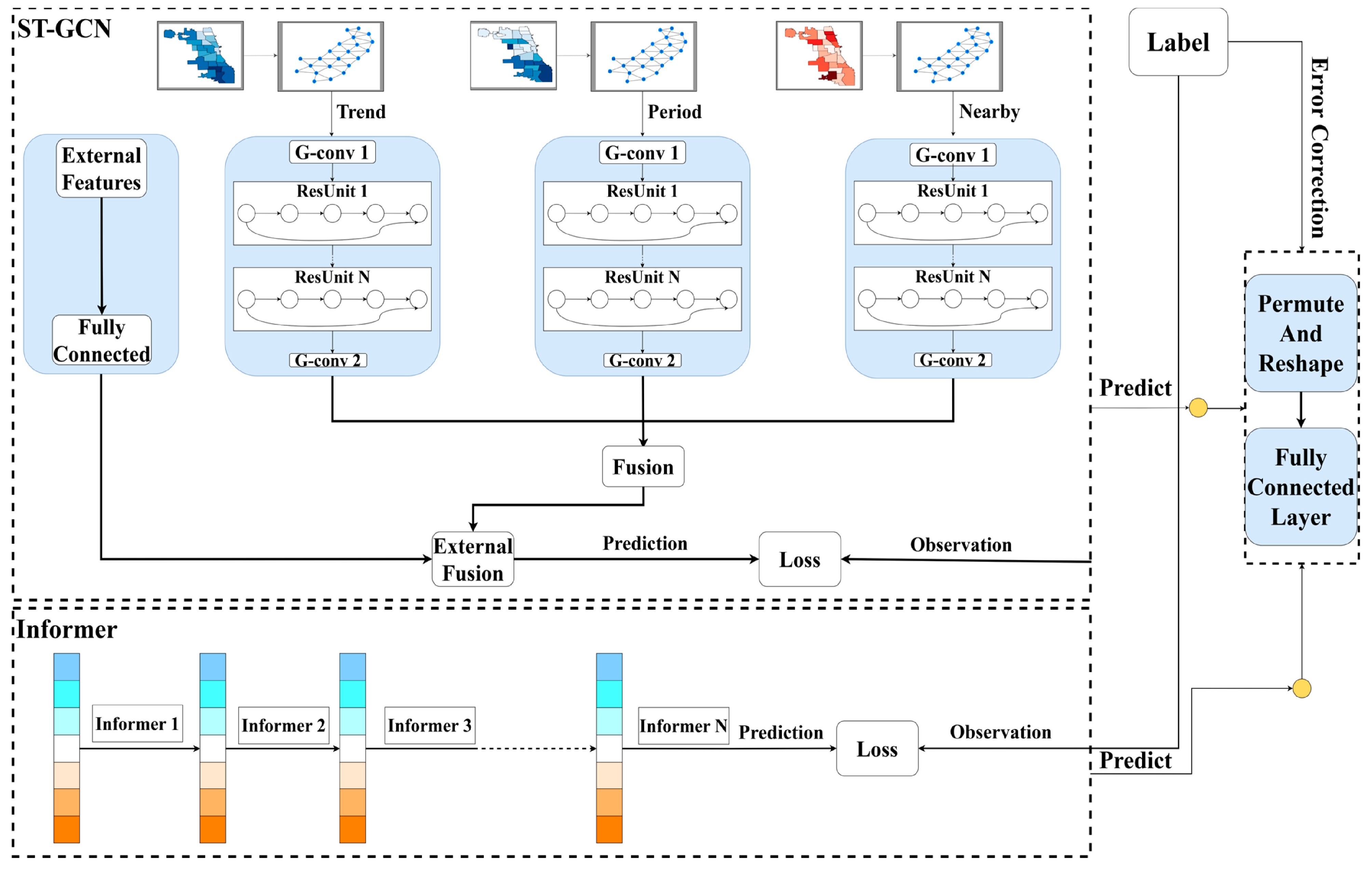
• Second, ST-GCN is used to capture the complex spatiotemporal transition trends of crime, while the Informer method is utilized to evaluate the temporal crime trends.
• Finally, through Convolutional Neural Networks (CNNs), the spatiotemporal and temporal features are integrated to construct a powerful spatiotemporal crime prediction model. This model, rooted in detailed community topological graphs and robust organized crime data, provides solid theoretical and data support for crime prediction.

The rest of this paper is organized as follows: Section 1 provides the research background. Section 2 describes the data and methods used. Section 3 presents and discusses the results. Finally, Section 4 offers our conclusion and future research directions.

2. Materials and Methods

2.1. Data Description

The data description includes data collection and data processing. First, to handle variations in crime across regions and enhance statistical reliability, we gathered data from 22 police districts in Chicago. Also, to address the issue of most prediction models, which focus solely on a single type of crime, we considered four major types of urban crimes: ‘Theft,’ ‘Criminal Damage,’ ‘Assault,’ and ‘Robbery.’ Data processing primarily involved three steps: handling missing data, generating feature data, and data integration. The major principles behind these processing steps are as follows:

• Addressing missing and abnormal data in the raw data;
• Generating non-obvious feature data based on existing data;
• Merging crime data with temperature data.

The features used are shown in

Table 1. Value description of external features.

Feature Name	Feature Value	Data Type
Date	The moment when the crime occurred	Date
Weekend	1-Weekday, 0-Weekend	Boolean
Holiday	1-Holiday, 0-Workday	Boolean
Weekday_avg	Average number of crime occurrences on weekdays	Float
Weekend_avg	Average number of crime occurrences on non-weekdays	Float
Month_avg	Average number of monthly crime occurrences	Float
Count_avg	Number at the previous moment	Int
T	Air temperature	Float
RH	Relative humidity	Float
V	Wind speed	Float
e	Water vapor pressure	Float
U	Relative humidity is indicated in the raw data	Float
Ff	Wind speed is indicated in the raw data	Float

.

2.1.1. Data Collection

We focused on relevant crime data from Chicago, conducting an in-depth analysis of a dataset spanning roughly five years, from 2015 to 2020, and encompassing an estimated 320,000 crime occurrences. These data were sourced from Chicago’s Open Data Portal (https://data.cityofchicago.org/ (accessed on 15 January 2025), a comprehensive online framework that provides abundant data resources on the city and includes various visualization tools, including maps and charts, to enable users to freely download the required data. The crime data were collected from the “Crimes—2001 to Present” dataset, which is a real collection of crime occurrences in Chicago from 2001 to the present. We selected 22 police districts in Chicago, with the largest being the 16th District (Jefferson Park), with an area of 30.95 square miles, and the smallest is the 23rd District (Town Hall), with an area of 3.01 square miles. From this dataset, we collected all of the crime occurrences within the aforementioned police districts over a period of just over 5 years (1895 days), from 1 January 2015, to 10 March 2020.

Based on the International Classification of Crime for Statistical Purposes (ICCS), we inferred four crime types from the crime data (https://nap.nationalacademies.org/read/23492/chapter/7/ (accessed on 23 January 2025)): assault, robbery, criminal damage, and theft. Additionally, we observed that the data contain detailed information for each crime occurrence, including the latitude and longitude of the crime and a description of the specific crime occurrence. Thus, we systematically classified the crime data based on this information and the national definitions of the laws.

The weather data used for our analysis were retrieved from the comprehensive Global Weather Database and downloaded from the website (http://rp5.ru/) (accessed on 28 January 2025). This database is known for its reliability and accuracy, acting as a pivotal source for meteorological information. The weather data in this database undergo rigorous checks every four hours, or six times per day, ensuring that the maximum, minimum, and average temperatures at the six designated time points align exactly with those recorded by official U.S. weather stations. This rigorous process is imperative for maintaining the consistency and accuracy of the data. Moreover, the temperature readings from our data source deviate by less than 1 °C from the official U.S. data, emphasizing the impressive reliability of the dataset. This minimal error margin serves as a testament to the robustness and trustworthiness of the weather data provided in this study.

2.1.2. Data Processing

Data processing included three critical steps. First, to address gaps in the crime and temperature datasets, missing values were imputed. For temperature data, missing values were filled in by calculating the daily average temperature for each date. When data for a given date were missing, we took a meticulous approach, calculating the average temperature over a 30-day period before and after the missing data point to ensure accurate inferences and factoring in the surrounding temporal context. For crime data, the daily number of crimes was ascertained. If no crimes were recorded for a particular date, a zero was explicitly added to assure the temporal integrity of the dataset. For crime data that does not have geographic information, we exclude it as anomalous data.

Second, we processed the feature data. Prior studies have shown that time factors exert a significant impact on crime rates. The temporal external feature used in this study was holiday data (represented by the feature “weekend”). Holidays included two scenarios. One was whether the day was a weekend or a weekday, indicated by the “weekend” feature, which was classified into two types. If the day was a weekend, the feature value was 1; otherwise, the value was 0. The other was whether the day was a statutory holiday, indicated by the “holiday” feature, also classified into two types. If the day was a statutory holiday, the feature value was 1; otherwise, it was 0. For the determination of whether a day was a statutory holiday, we used a list of statutory holidays in the U.S., obtained through research, and formulated judgment rules based on this list. In addition, we accounted for weather variables related to certain types of crimes. In this study, we used a discomfort index (DI) based on apparent temperature (AT) and thermodynamic wet-bulb temperature ($T_w$) as the weather data in our external features. The formulas for the corresponding characteristics are provided in Appendix A.

Last, we classified the crime data and temperature data and rigorously verified the accuracy of dates to ensure each timestamp’s accuracy. Then, we merged these datasets by matching them according to dates, and we adopted robust methods to handle format differences, thereby achieving seamless data integration. This approach established a foundation for analyzing the correlation between crime rates and temperature changes. The merged dataset enables comprehensive and multidimensional analysis, providing new insights into the influence of environmental factors on crime trends.

2.2. Methods

Figure 1 presents our proposed integrated model, which consists of three main modules: the spatiotemporal feature extraction module, temporal feature extraction module, and feature integration module. First, the spatiotemporal feature extraction module employs ST-GCN to extract spatial transition features of crimes over time. Second, the temporal feature extraction module builds upon the Informer network, aiming to detect criminal behavior features in each police jurisdiction. Last, the temporal latitude is aggregated with the space. The last time step of the encoder output is taken, and the features are mapped to the predicted latitude using a fully connected layer.

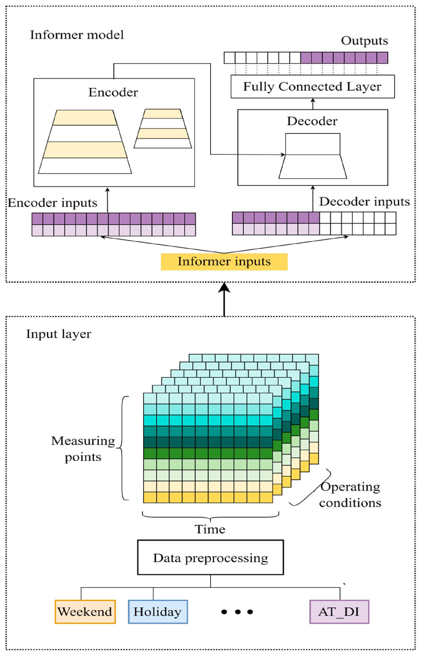
2.2.1. Informer Time Feature Extraction Module

When the Informer’s time feature extraction module computes the number of crimes, crime occurrences are collected as timing data. To process the timing data precisely, the Informer model, a self-attention-based architecture, is used. The Informer model can effectively capture long-range dependencies in serial data by processing all of the inputs at the same time during training, representing a significant improvement over traditional RNNs and their variants, such as LSTM networks. Figure 2 depicts the flowchart of the time feature extraction module.

The Informer model leverages three core components for efficient long-sequence forecasting: ProbSparse self-attention, self-attentional distilling, and a generative decoder.

The ProbSparse self-attention mechanism can efficiently compute attention scores by honing in on the most relevant input-output pairs. The ProbSparse Self-Attention mechanism begins by calculating a sparsity measure for each query vector. This measure helps identify the most relevant time points in the key vectors. The formula for the sparsity measure is as follows:

$$\overline{\mathrm{M}}\left(q_i,K\right)=MC-AC$$

(1)

where $q_i$ is the i-th query vector, and K is the set of key vectors. MC represents the maximum attention score between the query and any key vector. AC is the average attention score. The difference between these two terms indicates the “sparsity” of the attention distribution, with higher values suggesting that the query is more likely to focus on a few key vectors. The formulas for the MC and AC are as follows:

$$MC=\underset{j}{\max }\left\{{\displaystyle \frac{q_i{k}_j^T}{\sqrt{d}}}\right\}$$

(2)

$$AC={\displaystyle \frac{1}{L_K}}{\displaystyle \sum _{j=1}^{L_K}\frac{q_i{k}_j^T}{\sqrt{d}}}$$

(3)

where d is the dimensionality of the query and key vectors, and $L_k$ is the number of key vectors.

Based on the sparsity measure, the mechanism selects the top u queries with the highest sparsity scores. These queries are considered “active” and will be used to compute attention scores. The selection process ensures that only the most relevant queries are retained, significantly reducing the number of attention calculations. The attention scores are calculated using the scaled dot-product, which is expressed as follows:

$$\mathrm{Attention}\left(Q,K,V\right)=\mathrm{Softmax}\left({\displaystyle \frac{\tilde{Q}{K}^T}{\sqrt{d}}}\right)V$$

(4)

where $\tilde{Q}$ is the set of active query vectors, and V is the set of value vectors.

This approach reduces the time and space complexity from $O\left(L_Q{L}_K\right)$ to $O\left(L_{Q}ln{L}_K\right)$, enabling efficient long-sequence processing. In addition to reducing computational complexity, ProbSparse Self-Attention also improves memory efficiency. By focusing only on the most relevant time points, the model requires less memory to store intermediate results. This is particularly beneficial when dealing with long sequences, where memory constraints can be a significant issue.

Further enhancing the model’s ability to process long sequences, the Informer model uses a self-attentional distilling operation. This operation decreases the temporal dimension of the input sequence, enabling the encoder to process longer sequences efficiently. The distilling operation is as follows:

$$X_{t+1}=\mathrm{MaxPool}\left(\mathrm{Conv}1\mathrm{D}\left(X_t\right)\right)$$

(5)

where $X_t\in R^{L\times d}$, and $X_t$ denotes the encoder layer output at distillation step t. The 1D convolution (kernel size = 3) extracts local features, while max-pooling (stride = 2) halves the temporal dimension. This hierarchical distillation progressively removes redundant information while keeping critical attention patterns, decreasing memory usage by 50% per layer.

The generative decoder in the Informer model consists of two identical multi-head attention layers, which can effectively handle long inference processes without significant speed drops. The decoder input vector is calculated as follows:

$$D_{\mathrm{input}}=\mathrm{Concat}\left(\left[X_{\mathrm{token}},X_0\right]\right)\cdot W_{\mathrm{d}}+P_{\mathrm{d}}$$

(6)

where $X_{\mathrm{token}}\in R^{L_{\mathrm{token}}\times d}$, $X_0\in R^{L_y\times d}$, $P_{\mathrm{d}}\in R^{\left(L_{\mathrm{token}}+L_y\right)\times d}$, and $W_{\mathrm{d}}\in R^{2d\times d}$. $X_{\mathrm{token}}$ is a placeholder sequence initialized with zeros, $X_0$ is the target sequence positional embedding, $W_{\mathrm{d}}$ is a learnable projection matrix, and $P_{\mathrm{d}}$ is the decoder positional encoding. This design enables parallel generation of all of the prediction steps ($L_y$ time points) in one forward pass, avoiding the cumulative errors of autoregressive models.

Collectively, these architectural components enable Informer to project crime timing data into a latent representation space, where self-attention mechanisms effectively capture long-range temporal dependencies while circumventing the vanishing gradient issues inherent in RNNs. This is critical for predicting crime trends from historical data.

2.2.2. The Spatiotemporal Feature Extraction Module

This module considers districts as a node in the graph structure, which integrates relevant characteristics from criminal history records. To successfully analyze this type of graph data, the module adopts the Spatiotemporal Graph Convolutional Network (ST-GCN) framework. Specifically, the graph structure data are processed through the Graph Convolutional Network (GCN) mechanism, and Spatiotemporal Residual Network (ST-ResNet) is introduced to more deeply explore the spatiotemporal dimensional features in each set of graph nodes.

As the number of future crime occurrences in various urban areas is influenced both by the historical number of crime occurrences over time and the number of crime occurrences in neighboring areas spatially, our model employs a GCN to assess network topology dependencies, thereby more accurately extracting the spatial correlation of crime occurrence numbers. GCN, established by Kipf and Welling [40], extends traditional convolutional operations to topological structures to process topological data in deep learning. The forward propagation computation of GCN is expressed in the following equation:

$$f\left(X,A\right)=\mathrm{ReLU}\left(\hat{D}-{\displaystyle \frac{1}{2}}\hat{A}\hat{D}-{\displaystyle \frac{1}{2}}XW+b\right)$$

(7)

where X is the feature matrix, A is the adjacency matrix with self-loops incorporated, D denotes its degree matrix, ReLU represents the activation function of the network, and W and b are the parameters of the network.

However, as the topology features a large number of nodes, we must consider the transitional effects among them. In this sense, numerous GCN layers are required to capture further transitional effects from long-term or even city-wide dependencies, necessitating an extremely deep network architecture. Furthermore, the transitional nature of a crime is influenced both by neighboring features and by periodic and trend features. Thus, it is necessary to use ST-ResNet as the backbone model to host GCN layers (ST-GCN).

ST-ResNet, proposed by Zhang [41] based on deep Residual Network (ResNet) [42], can overcome the problems of inefficient learning and the inability to significantly improve accuracy or even to reduce accuracy due to network deepening. To more accurately capture the spatiotemporal crime distribution patterns, the ST-GCN model extracts three types of crime spatiotemporal features: “proximity features,” “periodic features,” and “trend features.” Specifically, to predict the number of crime occurrences on a certain day, the model extracts the number of crime occurrences from the three preceding days as proximity features; the number of crime occurrences from the 7th, 14th, and 21st days before that date as periodic features; and the number of crime occurrences from the same day three years prior as trend features.

The proposed crime prediction architecture integrates the Informer and ST-GCN models through a feature-level fusion mechanism. This integration leverages the complementary strengths of both approaches. Specifically, the Informer module excels at capturing long-range temporal dependencies across city-wide crime sequences, while the ST-GCN module effectively models localized spatiotemporal interactions between urban districts.

2.2.3. Evaluation

The Informer and ST-GCN model processes the training input features of dimension (1817, 22, 8, 5) and the testing input features of dimension (7, 8, 22, 5). It uses an adjacency matrix of size (22, 22) to capture the spatial relationships. The STGCN component transforms the spatial features into a 128-dimensional hidden space. After reshaping, these features are fed into the Informer model with a model dimension of 64 and 4 encoder layers to capture temporal patterns. The feature fusion mechanism merges the spatial and temporal dimensions to form the input for the final fully connected layer, which generates predictions reshaped to match the label dimensions (1817, 22) for training and (7, 22) for testing. The results from the two sets of models are then input into a final fully connected layer for fusion. The model employs a grid search method to optimize parameters and uses RMSE as the loss function. The NAdam optimizer is utilized for optimization, with an initial learning rate of 0.01, which is adjusted via cosine annealing. The training will terminate if the loss value does not decrease after 100 rounds.

In this study, we employed two core metrics to comprehensively assess model performance: mean absolute error (MAE) and RMSE. These metrics play essential roles in evaluating the model’s prediction accuracy, error magnitude, and relative error. Specifically, RMSE measures the square root of the sum of squared differences between the predicted and actual values. The equations for MAE and RMSE are as follows:

$$\mathrm{MAE}={\displaystyle \frac{1}{n}}{\displaystyle {\sum }_{i=1}^n\left|y_i-y_j\right|}$$

(8)

$$\mathrm{RMSE}=\sqrt{{\displaystyle \frac{1}{n}}{\displaystyle \sum _{i=1}^n{\left(y_i-y_j\right)}^2}}$$

(9)

where n is the total number of days, $y_i$ is the actual value, and $y_j$ is the predicted value.

At the same time, in order to directly quantify the model’s ability to explain the fluctuation of crime data and rigorously verify whether the MAE and RMSE are statistically significant when the MAE and RMSE are slightly improved, we also introduce the pair t-test and coefficient of determination (${\mathrm{R}}^2$) as auxiliary judgments.

To thoroughly demonstrate the superior performance of our model, we performed a robust comparison with various mainstream models, including the linear regression model, exponential smoothing model, ridge regression (Ridge) model, random forest model, LSTM model, Informer model, and LSTM-STGCN model. Through this series of comparative analyses, we aimed to uncover the significant advantages of our model in prediction accuracy, stability, and applicability.

3. Results

In this section, we present and analyze the experimental results and assess the performance of the proposed models for each community and each different type of crime on a daily basis using the test dataset. The test dataset covers the period from 1 January 2020, to 7 January 2020. Our discussion mainly focuses on the predictive performance of the models.

From Figure 3, the left panels show the original crime data; the middle panels, the prediction of the number of crimes; and the right panels, the absolute error between prediction and observation. Moreover, the bottom panels show the accumulations for the number of crimes and MAE from 1 January 2020, to 7 January 2020. For assaults, the model prediction performance was the best, achieving an average MAE of 0.42. Specifically, the remote District 15 achieved an MAE as low as 0.04, while District 16 achieved an MAE of 1.2, possibly due to the high unpredictability and weak historical regularity of public security incidents in District 16. For criminal damages, the average MAE was 0.85, with District 12 achieving an MAE of only 0.1, indicating that the model effectively captured the stable patterns of vandalism in this area. However, in District 22, the MAE rose to 2.26 due to infrastructure renovations, reflecting the interference of long-term environmental changes on predictions. Robberies ranked second in performance, with an average MAE of 0.45. The excellent performance in District 20, with an MAE of 0.08, may stem from the high-quality data supported by comprehensive surveillance coverage. In contrast, Districts 11 and 18 had MAEs exceeding 1.4, suggesting the complexity of crime patterns in densely populated areas with high mobility. Thefts exhibited the greatest prediction challenge, achieving an average MAE of 1.36. The eastern coastal District 1 had an MAE reaching as high as 4.46, associated with the diverse criminal motives and high incidence of crimes in public places such as hospitals and parks. Conversely, the MAE of 0.3 in the southeastern District 5 demonstrated the model’s adaptability to regular commercial thefts.

The spatial distribution of prediction errors revealed the considerable influence of public security environments and data characteristics (Figure 4). Specifically, developed areas (e.g., Coastal District 1) exhibited prediction fluctuations due to complex human flow dynamics and diverse criminal triggers, while remote regions (e.g., Southeast District 4) were likely constrained by data sparsity and public security instability. High errors were concentrated in two types of scenarios: areas dominated by sudden events (e.g., violent incidents in District 16) and areas undergoing long-term environmental changes (e.g., construction impacts in District 22). To enhance model robustness, we integrated real-time emergency data with dynamic environmental features.

As shown in Figure 5, the prediction results based on the Informer and ST-GCN fusion model indicate that the actual number of assaults exhibited significant non-periodic fluctuation characteristics. However, the model still effectively captured the dynamic trends in the number of crime occurrences across 22 police jurisdictions. Specifically, in terms of spatial feature extraction, the ST-GCN module successfully captured the correlations in crime patterns across jurisdictions, resulting in a 95.2% overlap between the predicted curve for Jurisdiction 15 (red dashed line) and the actual observations (blue solid line), with an MAE of 0.04, significantly outperforming traditional time series models. For the sudden increase in Jurisdiction 4 on 6 January (with a single-day increase of 64.5% in the number of crime occurrences), the Informer module accurately identified this abnormal fluctuation pattern using its ProbSparse self-attention mechanism, predicting a 58.3% increase from the previous day, with the error in the actual increase being controlled within a range of ±6.2%. Although the prediction error for Jurisdiction 16 was relatively large, the model still correctly predicted the crime trend, demonstrating its good performance in predicting non-monotonic trends.

4. Discussion

We employed the evaluation metrics MAE and RMSE to quantitatively assess the performance of the Informer and ST-GCN model on the prediction dataset. The results were compared with those of ARIMA, Ridge Regression, Support Vector Regression (SVR), Random Forest, XGBoost, LSTM, Convolutional Neural Network (CNN), Convolutional Long Short-Term Memory (Conv-LSTM), and LSTM and ST-GCN (LSTM-STGCN) on the same dataset, as shown in

Table 2. Comparison of model prediction results (with theft as an example).

Model	MAE	RMSE	${\mathbf{R}}^2$
ARIMA	3.42	3.98	0.43
Ridge Regression	3.13	3.61	0.45
SVR	2.91	3.43	0.48
Random Forest	2.42	2.89	0.54
XGBoost	2.46	2.95	0.53
LSTM	1.86	2.44	0.72 *
CNN	1.44	1.76	0.76 *
Informer	1.45	1.78	0.75 *
Conv-LSTM	1.42	1.72	0.81 *
LSTM-STGCN	1.38	1.68	0.82 *
Our Model	1.36	1.65	0.83 *

* Denotes a significance level lower than 0.05.

,

Table 3. Comparison of model prediction results (with assault as an example).

Model	MAE	RMSE	${\mathbf{R}}^2$
ARIMA	1.83	2.24	0.45
Ridge Regression	1.56	1.97	0.49
SVR	1.42	1.91	0.50
Random Forest	1.37	1.68	0.51
XGBoost	1.29	1.63	0.54
LSTM	1.18	1.43	0.71 *
CNN	0.93	1.13	0.78 *
Informer	1.10	1.38	0.74 *
Conv-LSTM	0.89	1.06	0.82 *
LSTM-STGCN	0.82	0.94	0.83 *
Our Model	0.73	0.89	0.86 *

* Denotes a significance level lower than 0.05.

,

Table 4. Comparison of model prediction results (with robbery as an example).

Model	MAE	RMSE	${\mathbf{R}}^2$
ARIMA	2.47	3.04	0.44
Ridge Regression	2.13	2.62	0.47
SVR	2.07	2.51	0.49
Random Forest	1.84	2.35	0.54
XGBoost	1.81	2.28	0.55
LSTM	1.45	1.77	0.76 *
CNN	1.26	1.49	0.78 *
Informer	1.25	1.47	0.78 *
Conv-LSTM	1.12	1.35	0.83 *
LSTM-STGCN	1.06	1.22	0.84 *
Our Model	1.03	1.17	0.84 *

* Denotes a significance level lower than 0.05.

and

Table 5. Comparison of model prediction results (with criminal damage as an example).

Model	MAE	RMSE	${\mathbf{R}}^2$
ARIMA	2.65	3.15	0.45
Ridge Regression	2.46	2.87	0.48
SVR	2.28	2.66	0.49
Random Forest	1.73	2.02	0.58
XGBoost	1.74	2.05	0.58
LSTM	1.15	1.46	0.75 *
CNN	1.12	1.39	0.78 *
Informer	1.11	1.38	0.78 *
Conv-LSTM	1.06	1.28	0.82 *
LSTM-STGCN	1.04	1.22	0.83 *
Our Model	1.05	1.24	0.83 *

* Denotes a significance level lower than 0.05.

.

For the 22 police jurisdictions, our model’s worst prediction error for the number of thefts was less than 2 per day (MAE = 1.36, RMSE = 1.65); the model’s prediction error for the number of assaults was the smallest, at less than 1 per day (MAE = 0.73, RMSE = 0.89). In addition, for robbery, the results were MAE = 1.03 and RMSE = 1.17. For criminal damage, they were MAE = 1.05 and RMSE = 1.24. Overall, these results indicate that the Informer and ST-GCN model possesses good spatiotemporal crime prediction capabilities. Compared with other models, this model exhibited superior performance in terms of both MAE and RMSE. Furthermore, as shown in Table 2, Table 3 and Table 4, the performance of ARIMA, Ridge Regression, SVR, Random Forest, and XGBoost was significantly worse than that of the deep learning models LSTM, CNN, and Conv-LSTM. In addition, we tested the significance level of the regression model. The significance levels of LSTM, Informer, CNN, and the ensemble model were all below 0.05, whereas traditional machine learning models such as SVR showed significance levels exceeding 0.05. This indicates that the regression results of our proposed ensemble model are statistically significant and demonstrate greater reliability compared to conventional approaches. This may be because SVR and other statistical-based models, as well as traditional machine learning models, struggle to extract complex high-dimensional spatiotemporal features from crime statistics. Among the deep learning models, LSTM’s performance was notably lower than that of CNN and Conv-LSTM, which are more adept at capturing spatial autocorrelation in crime occurrences. The model proposed in this paper outperformed the other three deep learning models in prediction results. This may be because the other three deep learning models are based on regular spatiotemporal grids for spatial division, and many potential spatial correlation features between actual irregular administrative divisions cannot be effectively extracted. In contrast, the proposed model, which integrates the ST-GCN model, uses ResNet and GCN to extract the topological relationships among the 22 police jurisdictions in the city. It then fuses these features using an attention mechanism that weights and computes complex features, thus enabling more accurate prediction of the spatiotemporal distribution of crime.

Our proposed hybrid architecture synergistically integrates Informer and ST-GCN modules. Informer leverages its probabilistic sparse attention mechanism to process extended spatiotemporal sequences, effectively capturing long-range temporal dependencies in crime pattern evolution. Concurrently, ST-GCN incorporates graph convolutional layers to model spatial correlations through dynamic topological representations of regional interactions. This dual-mechanism design enables two-fold interpretability enhancement:

• Informer’s multi-head self-attention quantifies temporal contribution weights across different time windows and geographic zones, providing traceable temporal-spatial attribution for crime forecasts.
• ST-GCN’s graph attention networks reveal inter-regional influence patterns by learning adaptive edge weights between graph nodes, thereby elucidating complex spatial dependencies that conventional grid-based approaches overlook.

The complementary fusion of these mechanisms not only improves predictive accuracy but also constructs a transparent decision-making framework for crime trend analysis.

5. Conclusions

In conclusion, our model achieves exceptional precision for violent crimes, notably reducing assault prediction errors to MAE = 0.73—45% lower than the best traditional model and surpassing all comparative baselines. For assault prediction, our model achieves quantitative supremacy with 8.7% lower MAE than LSTM-STGCN, 6.3% reduced RMSE versus Conv-LSTM, and R² = 0.86. Furthermore, for the other three crime types, while substantial reductions in MAE and RMSE were not achieved, paired t-tests revealed statistically significant differences (p < 0.05) between our model and the other two hybrid baselines.

The experimental results indicate that our proposed crime prediction model excels in its capacity to discern intricate temporal patterns intrinsic to individual communities while simultaneously capturing the complex spatiotemporal interdependencies between adjacent areas. This dual proficiency enables the model to render precise predictions of daily crime occurrences across a spectrum of categories, offering a granular perspective on the evolution of various crime types through time and space.

The robustness of this integrated model stems from its harmonious assimilation of long-range temporal dependencies, as captured by the Informer component, with the spatiotemporal correlations modeled by the ST-GCN architecture. This synergistic interplay augments the model’s ability to learn from historical crime trajectories and also efficiently integrates the influence of transitional criminal activities across contiguous regions. Consequently, the model attains a more accurate depiction of crime dynamics compared with isolated models, presenting a resilient framework for the prediction of multifarious crime types. The implications of this study are profound, offering urban planners and law-enforcement agencies data-driven insights for optimizing resource allocation strategies for crime prevention and control. Based on the results of the study, policymakers can rank their own forecasts. When elevated crime risk is predicted, multi-modal policing strategies must be deployed to maintain operational safety. The goal is to develop a hybrid resource allocation scheme that simultaneously minimizes expected crime risk escalation and policing costs. This requires balancing spatial-temporal resource distribution through optimization techniques to achieve cost-effective risk mitigation.

Despite our model achieving good results, several avenues for future research are available. Our experimental results indicate that, although the model exhibits considerable resilience, its performance remains susceptible to fluctuations in social variables within certain communities. Therefore, future investigations should consider expanding the repertoire of external features beyond meteorological and temporal indicators, integrating supplementary socioeconomic metrics to further enhance predictive precision and model robustness. On the other hand, conducting sensitivity analysis of the model to input variables and quantifying feature importance coefficients represent critical pathways for advancing predictive science in future research. In addition, the complexity of the model architecture poses challenges, as it may induce training difficulties in managing multi-type crime predictions.

Moving forward, the emphasis of future research should be on refining the model to achieve an optimal equilibrium between effectiveness and simplicity. This effort encompasses exploring methodologies to incorporate more diverse external data sources while also simplifying the model’s architecture to preserve its predictive potency. Such advancements may produce more versatile, pragmatic instruments for urban crime analysis, thus fostering the creation of safer and more habitable communities.

References

1. Kornec, R. Ecological security of communities in polish cities. J. Plant Growth Regul. 2020, 16, 41–50. [Google Scholar] [CrossRef]
2. Andresen, M.A.; Linning, S.J.; Malleson, N. Crime at places and spatial concentrations: Exploring the spatial stability of property crime in Vancouver BC, 2003–2013. J. Quant. Criminol. 2017, 33, 255–275. [Google Scholar] [CrossRef]
3. Hegewald, S. Locality as a safe haven: Place-based resentment and political trust in local and national institutions. J. Eur. Public Policy 2023, 31, 1749–1774. [Google Scholar] [CrossRef]
4. Chen, Y. Research on influencing factors of local epidemic prevention and control policy making: Based on the fuzzy set qualitative comparative analysis of 46 cities aiming at Chengdu’s epidemic prevention and control policies. In Proceedings of the 7th International Conference on Humanities and Social Science Research (ICHSSR 2021), Qingdao, China, 23–25 April 2021; pp. 140–143. [Google Scholar]
5. Ravi Kumar, P.; Jayaram, A.; Somashekar, R. Assessment of the performance of different compost models to manage urban household organic solid wastes. Clean Technol. Environ. Policy 2009, 11, 473–484. [Google Scholar] [CrossRef]
6. Vaccaro, A.; Popov, M.; Villacci, D.; Terzija, V. An integrated framework for smart microgrids modeling, monitoring, control, communication, and verification. Proc. IEEE 2010, 99, 119–132. [Google Scholar] [CrossRef]
7. Liao, W.; Huang, X.; Van Coillie, F.; Gautama, S.; Pižurica, A.; Philips, W.; Liu, H.; Zhu, T.; Shimoni, M.; Moser, G.; et al. Processing of multiresolution thermal hyperspectral and digital color data: Outcome of the 2014 IEEE GRSS data fusion contest. IEEE J. Sel. Top. Appl. Earth Obs. Remote Sens. 2015, 8, 2984–2996. [Google Scholar] [CrossRef]
8. Qiu, J.; Zhuang, L.; Zhou, Y.; Duan, Z. A standard cloud platform technology of traffic performance index based on multi-source data fusion. Open J. Trans. Technol. 2018, 7, 340–350. [Google Scholar] [CrossRef]
9. Muchwanju, C.; Chelule, J.C.; Mung’Atu, J. Modelling crime rate using a mixed effects regression model. Am. J. Theor. Appl. Stat. 2015, 4, 496–503. [Google Scholar] [CrossRef]
10. Cohen, L. Social change and crime rate trends: A routine activity approach. Am. Sociol. Rev. 1979, 44, 588–608. [Google Scholar] [CrossRef]
11. Johnson, S.D.; Bowers, K.; Hirschfield, A. New insights into the spatial and temporal distribution of repeat victimization. Br. J. Criminol. 1997, 37, 224–241. [Google Scholar] [CrossRef]
12. Eysenck, H.J.; Gudjonsson, G.H. Crime and personality. In The Causes and Cures of Criminality; Springer: New York, NY, USA, 1997; pp. 43–89. [Google Scholar]
13. Clarke, R.V.G.; Felson, M. Routine Activity and Rational Choice; Routledge: Piscataway, NJ, USA, 1993. [Google Scholar]
14. Hadzikadic, M.; Carmichael, T.; Curtin, C. Complex adaptive systems and game theory: An unlikely union. Complexity 2010, 16, 34–42. [Google Scholar] [CrossRef]
15. Mohamad, A.M.; Hamin, Z.; Nor, M.Z.M.; Aziz, N.A. Selected theories on criminalisation of hacking. Int. J. Law Gov. Commun. 2021, 6, 168–178. [Google Scholar] [CrossRef]
16. Tolulope, O.O. Students’ predisposition to being a victim of internet crime in tertiary institutions of Nigeria. Cult. Commun. Social. J. 2022, 3, 44–48. [Google Scholar] [CrossRef]
17. Shiode, N.; Shiode, S.; Nishi, H.; Hino, K. Seasonal characteristics of crime: An empirical investigation of the temporal fluctuation of the different types of crime in London. Comput. Urban Sci. 2023, 3, 19. [Google Scholar] [CrossRef]
18. Breetzke, G.D.; Cohn, E.G. Seasonal assault and neighborhood deprivation in South Africa: Some preliminary findings. Environ. Behav. 2012, 44, 641–667. [Google Scholar] [CrossRef]
19. Tang, Y.; Zhu, X.; Guo, W.; Wu, L.; Fan, Y. Anisotropic diffusion for improved crime prediction in urban China. ISPRS Int. J. Geo-Inf. 2019, 8, 234. [Google Scholar] [CrossRef]
20. Wang, Z.; Liu, X. Analysis of burglary hot spots and near-repeat victimization in a large Chinese city. ISPRS Int. J. Geo-Inf. 2017, 6, 148. [Google Scholar] [CrossRef]
21. Reid, A.A.; Frank, R.; Iwanski, N.; Dabbaghian, V.; Brantingham, P. Uncovering the spatial patterning of crimes: A criminal movement model (CriMM). J. Res. Crime Delinq. 2014, 51, 230–255. [Google Scholar] [CrossRef]
22. Yang, M.; Chen, Z.; Zhou, M.; Liang, X.; Bai, Z. The impact of COVID-19 on crime: A spatial temporal analysis in Chicago. ISPRS Int. J. Geo-Inf. 2021, 10, 152. [Google Scholar] [CrossRef]
23. Monish, N. Chicago crime analysis using r programming. Int. J. Sci. Res. Comput. Sci. Eng. Inform. Technol. 2019, 5, 937–944. [Google Scholar] [CrossRef]
24. Shen, H.L.; Zhang, H.; Zhang, Y.F.; Zhang, Z.G.; Zhu, Y.M.; Cai, L. Prediction of burglary crime based on LSTM. J. Stat. Inform. 2019, 34, 107–115. [Google Scholar] [CrossRef]
25. Zhuang, Y.; Almeida, M.; Morabito, M.; Ding, W. Crime hot spot forecasting: A recurrent model with spatial and temporal information. In Proceedings of the 2017 IEEE International Conference on Big Knowledge (ICBK), Hefei, China, 9–10 August 2017; pp. 143–150. [Google Scholar]
26. Yan, S.; Xiong, Y.; Lin, D. Spatial temporal graph convolutional networks for skeleton-based action recognition. In Proceedings of the AAAI Conference on Artificial Intelligence, New Orleans, LA, USA, 2–7 February 2018; pp. 7444–7452. [Google Scholar]
27. Gao, Z.; Yang, R.; Zhao, K.; Yu, W.; Liu, Z.; Liu, L. Hybrid convolutional neural network approaches for recognizing collaborative actions in human-robot assembly tasks. Sustainability 2024, 16, 139. [Google Scholar] [CrossRef]
28. Zhao, D.; Du, P.; Liu, T.; Ling, Z.F. Spatio-temporal distribution prediction model of urban theft by fusing graph autoencoder and GRU. J. Geo-Inform. Sci. 2023, 25, 1448–1463. [Google Scholar] [CrossRef]
29. Han, X.G.; Hu, X.F.; Wu, H.; Shen, B.; Wu, J. Risk prediction of theft crimes in urban communities: An integrated model of LSTM and ST-GCN. IEEE Access 2020, 8, 217222–217230. [Google Scholar] [CrossRef]
30. Hu, J.M.; Hu, X.F.; Han, X.G.; Lin, Y.; Wu, H.; Shen, B. Exploring the correlation between temperature and crime: A case-crossover study of eight cities in America. J. Saf. Sci. Resil. 2024, 5, 13–36. [Google Scholar] [CrossRef]
31. Pleshakova, E.; Osipov, A.; Gataullin, S.; Gataullin, T.; Vasilakos, A. Next gen cybersecurity paradigm towards artificial general intelligence: Russian market challenges and future global technological trends. J. Comput. Virol. Hack. Tech. 2024, 20, 429–440. [Google Scholar] [CrossRef]
32. Kalai Selvan, A.; Sivakumaran, N. Crime detection and crime hot spot prediction using the BI-LSTM deep learning model. Int. J. Knowl.-Based Dev. 2024, 14, 57. [Google Scholar] [CrossRef]
33. Fan, Q.; Xu, G. Real-time prediction model of public safety events driven by multi-source heterogeneous data. Front. Phys. 2025, 13, 1553640. [Google Scholar] [CrossRef]
34. Zhou, H.; Zhang, S.; Peng, J.; Zhang, S.; Li, J.; Xiong, H.; Zhang, W. Informer: Beyond efficient transformer for long sequence time-series forecasting. arXiv 2020, arXiv:2012.07436. [Google Scholar] [CrossRef]
35. Atero, F.J.; Vinagre, J.J.; Morgado, E.; Wilby, M.R. A low energy and adaptive architecture for efficient routing and robust mobility management in wireless sensor networks. In Proceedings of the 2011 31st International Conference on Distributed Computing Systems Workshops, Minneapolis, MN, USA, 20–24 June 2011; pp. 172–181. [Google Scholar]
36. Ya, M.A.; Yaw, C.; Koh, S.; Tiong, S.; Chen, C.; Yusaf, T.; Abdalla, A.; Ali, K.; Raj, A. Detection of corona faults in switchgear by using 1D-CNN, LSTM, and 1D-CNN-LSTM methods. Sensors 2023, 23, 3108. [Google Scholar] [CrossRef]
37. Xu, H.; Peng, Q.; Wang, Y.; Zhan, Z. Power-load forecasting model based on informer and its application. Energies 2023, 16, 3086. [Google Scholar] [CrossRef]
38. Yang, Z.; Liu, L.; Li, N.; Tian, J. Time series forecasting of motor bearing vibration based on informer. Sensors 2022, 22, 5858. [Google Scholar] [CrossRef] [PubMed]
39. Jun, J.; Kim, H.K. Informer-based temperature prediction using observed and numerical weather prediction data. Sensors 2023, 23, 7047. [Google Scholar] [CrossRef] [PubMed]
40. Davies, N.B.; Krebs, J.R.; West, S.A. An Introduction to Behavioural Ecology; Wiley: Hoboken, NJ, USA, 2012. [Google Scholar]
41. Zhang, J.; Zheng, Y.; Qi, D. Deep spatio-temporal residual networks for citywide crowd flows prediction. In Proceedings of the AAAI Conference on Artificial Intelligence, San Francisco, CA, USA, 4–9 February 2017; pp. 1655–1661. [Google Scholar]
42. He, K.; Zhang, X.; Ren, S.; Sun, J. Identity mappings in deep residual networks. In Proceedings of the Computer Vision-ECCV 2016: 14th European Conference, Amsterdam, The Netherlands, 11–14 October 2016; pp. 630–645. [Google Scholar]
Figure 1. The structure of the ensemble model, where blocks of different colors and yellow dots denote the input temporal data and predicted data, respectively.
Bdcc 09 00179 g001
Figure 2. Diagram of the end-to-end prediction process of the Informer model, including the input layer, encoder, decoder, and outputs.
Bdcc 09 00179 g002
Figure 3. Spatial distribution of the predicted number of crimes and mean absolute error (MAE) of different districts in Chicago.
Bdcc 09 00179 g003
Figure 4. Geographic comparison of crime occurrence counts across 22 Chicago Police Districts. Blue represents original data; orange represents predicted data.
Bdcc 09 00179 g004
Figure 5. The time distribution chart of the number of daily assaults predicted by the model.
Bdcc 09 00179 g005