Enhancing Drone Detection via Transformer Neural Network and Positive–Negative Momentum Optimizers

Abstract

The rapid development of unmanned aerial vehicles (UAVs) has had a significant impact on the growth of the economic, industrial, and social welfare of society. The possibility of reaching places that are difficult and dangerous for humans to access with minimal use of third-party resources increases the efficiency and quality of maintenance of construction structures, agriculture, and exploration, which are carried out with the help of drones with a predetermined trajectory. The widespread use of UAVs has caused problems with the control of the drones’ correctness following a given route, which leads to emergencies and accidents. Therefore, UAV monitoring with video cameras is of great importance. In this paper, we propose a Yolov12 architecture with positive–negative pulse-based optimization algorithms to solve the problem of drone detection on video data. Self-attention-based mechanisms in transformer neural networks (NNs) improved the quality of drone detection on video. The developed algorithms for training NN architectures improved the accuracy of drone detection by achieving the global extremum of the loss function in fewer epochs using positive–negative pulse-based optimization algorithms. The proposed approach improved object detection accuracy by 2.8 percentage points compared to known state-of-the-art analogs.

1. Introduction

In today’s world, unmanned aerial vehicles (UAVs) are becoming increasingly in demand and popular. They are used by both amateur photo and video shooters and large companies specializing in such areas as digital agriculture [1], geological exploration [2], construction [3], sensing [4], logistics [5], firefighting [6], monitoring [7], and others. The possibility of conducting video surveys in dangerous or hard-to-reach places for humans has entailed a huge flow of data, the processing of which requires advanced artificial intelligence methods. Detection and recognition of moving objects are the main tasks that machine learning solves in UAV operations. Drone detection to control their position in space, recognize the correctness of following a given route, and monitor compliance with rules in public places requires special attention. However, state-of-the-art methods for drone detection using video data do not provide sufficient quality for the assigned task performance. There are problems with recognizing objects on inhomogeneous backgrounds and with poor image quality. In [8], the authors use a cascaded Haar filter for object detection. This approach has low computational complexity and high speed but at the same time shows lower accuracy of object detection in video data than NN methods. Mask Region-Based Convolutional Neural Networks (Mask R-CNN) [9], a modification of Faster Region-Based Convolutional Neural Networks (Faster R-CNN) [10], are solving object detection and segmentation problems in visual data more accurately than wavelet approaches. This NN framework uses a multi-stage image-processing approach, analyzing each image multiple times. A more recent development is Yolov3 [11], which is one of the first versions of the You Only Look Once models. This NN is operated in real time without degrading the recognition accuracy. A later modification of Yolov3 is Yolov5 [12]. The main differences between this model and the earlier version are the use of Cross Stage Partial blocks instead of backbone blocks and the replacement of the feature pyramid network with a path aggregation network using Spatial Pyramid Pooling—Fast (SPPF). Yolov5 enables faster training, smaller model sizes, and higher accuracy. YoloX [13] is an anchor-free version of YOLO. This approach allows us to increase the speed of image processing by speeding up the process of bounding box detection. Yolov8 [14] is also used to solve this problem. This architecture uses a new approach in error estimation using several loss functions: box loss, distribution focus loss, and classification loss. Yolov8 is able to more accurately place bounding boxes around both large and small objects.

1.1. Motivation

State-of-the-art approaches to solving the problem of drone recognition in video data have many drawbacks. The Haar cascade filter does not allow for accurately determining the boundaries of the UAV due to the complex geometric shape of the object. Also, this filter is sensitive to shadows, glare, and the orientation of objects, which is critical in UAV recognition. Models based on Mask R-CNN consist of convolutional NNs and, in the process, use a two-stage detector, the first step finding areas with objects and the second classifying them. This approach increases the image-processing time, which does not allow Mask R-CNN to be used for real-time operation. Also, this architecture requires significant computational resources, which makes it difficult to use this method on a mass scale. Yolov3, Yolov5, and Yolov8 are earlier architectures in the Yolo series that exhibit lower accuracy than their newer and later counterparts. In this paper, we propose to use architectures based on Yolov11 [15] and Yolov12 [16] to solve the drone recognition problem. These architectures are cutting-edge in real-time object detection. Yolov11 is a CNN whose main feature is improved feature extraction using backbone and neck architecture, which achieves higher accuracy. Yolov12 differs from previous versions of Yolo in its feature extraction mechanism using the self-attention method [17], which has proven to be a reliable and efficient method in recent years.

However, advanced optimization algorithms are required, along with the use of advanced architectures. This is required to find the global minimum of the loss function in fewer training epochs. Stochastic gradient descent (SGD) [18] finds the minimum by considering the direction of the gradient. The adaptive moment estimation method with split weight reduction (AdamW) uses an exponential moving average of the gradient and its square. There are optimizers that combine the two previous approaches. AdaBelief [19] achieves this by introducing trust correction into the Adam algorithm. However, these methods do not distinguish local and global extrema, which prevents them from always reaching the global minimum. YogiPNM and DiffPNM can solve this problem and achieve the global minimum of the loss function in fewer epochs [20]. In this paper, we address the problem of UAV detection in videos. The widespread use of drones in many areas of human activity has created a need for their detection. Fast and accurate detection of drones can prevent accidents or invasion of private property. Moreover, such a detection system is used in UAVs themselves to prevent accidents with other drones during joint flights. The problem of detecting UAVs in a video data stream is usually solved using such models as R-CNN and Masked R-CNN. However, such NN models are outdated and structured on CNNs, which are devoted to pattern recognition problem-solving in images. The application of Yolov2–Yolov10 [21] model losses does not result in a significant increase in the precision, recall, F1-score, and other metrics. Besides the NN models, the optimization algorithms play a crucial role in object detection problem-solving. The standard optimizers, such as SGD, Adam, AdamW, DiffGrad, Yogi, and AdaBelief, attain the global minimum of the loss function for a large number of epochs or do not reach the extreme at all. Therefore, one needs to use new optimizers, which avoid local extremes and solve vanishing and exploding gradient problems. Considering the above facts, we decided to use Yolov11 and Yolov12 models with advanced optimization algorithms YogiPNM and DiffPNM. In this study, we show that Yolov11 and Yolov12 using these optimizers exhibit higher precision, recall, and F1-score values compared to models trained using SGD, AdamW, AdaBelief, Yogi, and Diffgrad.

1.2. Our Contribution

Our contributions are summarized as follows:

• Development of NN structures based on Yolov11 and Yolov12 models and YogiPNM and DiffPNM optimization algorithms to solve the problem of drone detection in video data streams.
• Improving the solution quality of the UAV detection problem in video data using the proposed machine learning models.
• Improving the learning rate of NNs solving the problem of UAV detection on video data by minimizing the loss function over a smaller number of epochs.

The proposed NN models based on Yolov11 and Yolov12 using YogiPNM and DiffPNM increased the value of precision, recall, mAP50, and F10-score metrics compared to their state-of-the-art analogs, minimizing the loss function using earlier optimization algorithms.

The technical contribution is the combination of positive–negative optimizers and a coordinate descent approach. The combination of gradient and coordinate descents allows the vanishing and exploding derivative to be solved, which periodically appears in loss function minimization. This feature is shown in test function minimization, where researchers test new optimizers for hyperparameter determination. Next, we integrate the proposed optimization algorithm into Yolov11 and Yolov12 models for drone detection solving. Our model attains a high value of precision, recall, F1-score, and other metrics for the smaller number of iterations than analogs with standard optimizers.

The rest of the paper is organized as follows. In Section 2, we provide the actual methods for solving the object detection problem. Section 3 describes both the Yolov11 and Yolov12 architectures and optimization methods. Section 4 describes the Yolov11 and Yolov12 models with positive–negative optimizers. Section 5 demonstrates the results of solving the drone detection problem using Yolo models and different optimization methods. Section 6 discusses further improvements and applications of the proposed Yolov11 and Yolov12 NNs. Lastly, Section 7 summarizes the conclusions and results of solving the UAV recognition problem using the proposed NNs.

2. Related Work

2.1. Object Detection

Many researchers and developers have solved the object detection problem in arbitrary visual data via modern deep learning models. R-CNN [9] is one of the first NNs that detects objects in various visual data. There exist many modifications of this network, such as Mask and Faster R-CNN [10] and R-CNN with a feature pyramid net [22], which increase the accuracy and time of solving an object detection problem, respectively. The main idea of the application of feature pyramid networks is layer sharing, where the backbone and additional net train the common layers. The addition of the mask method to this model significantly improves the quality of solving the object detection problem. However, R-CNN-type NNs have become outdated compared to new deep learning models.

An alternative approach for raising the quality of object detection is the single-shot multi-box detector (SSD) [23]. The authors customized such a model under CNNs, ResNet-50, ResNet-101, MobileNet v2, and Inception v2 to solve the problem of ripe fruit detection in the FAOSAT dataset. The SSD demonstrated higher precision, recall, F1-score, and mAP than known analogs. In [24], the authors proposed RetinaNet for detecting objects on the visual dataset COCO. This deep learning model consists of ResNet, a feature pyramid net, and class and box subnets. Such a model is the reason for the continuation of Faster R-CNN with a feature pyramid net. Another promising model is EfficientDet [25]. As the backbone, this NN contains ImageNet-pretrained EfficientNet with a bi-feature pyramid net. The EfficientDet demonstrated higher results in solving the object detection problem on visual state from the COCO dataset than SSD, Faster R-CNN, and Yolov2.

Demonstrated NNs are still being used to solve the object detection problem in various fields of human activity. However, they have many disadvantages, such as the utilization of outdated optimization algorithms and the use of ResNet, EfficientNet, and MobileNet as backbone networks. It results in losses in performance and a low convergence rate to the global minimum of the loss function. We proposed using the latest Yolo-type NN with advanced optimization algorithms. Yolov11 [15] has more adaptive architectures, which analyze the features of data more correctly and precisely than R-CNN, SSD, and EfficientDet because of the original backbone, neck, and head structures. The most recent Yolov12 [16] is based on the self-attention mechanism, which verifies the feature by tokens. At the moment, the Yolov11 and Yolov12 networks show the best quality of solving the object detection problem on arbitrary visual data. For solving the global loss function minimization problem, we propose using novel positive–negative momentum optimizers, which solve the vanishing gradient, exploding gradient, and local minimum convergence problems. Unlike traditional first-order optimizers based on gradient descent and adaptive moment estimation, these optimization algorithms have a higher convergence rate to the global minimum of the loss function. This feature allows us to raise the quality of solving the object detection problem.

2.2. Drone Detection

The UAV detection problem has remained unsolved for a long time. There exists much research devoted to solving this problem. The recent ways to solve the drone detection problem are divided into four branches [26]: radio-frequency-based UAVs, visual data (images/video)-based UAVs, acoustic/sound-based UAVs, and radar-based UAV detection. To solve this problem, many researchers and developers are applying modern AI methods such as support vector machines, deep learning, k-nearest neighborhoods, and random forests. In many articles, the authors use outdated machine learning methods. In paper [27], the authors use Yolov3 and R-CNN models for detecting drones in images. A more recent Yolov4 model was used to raise the quality of solving UAV detection in videos [28]. The deep clustering [29] approach in the Yolov8 model allowed the enhancement of drone detection in visual datasets compared with Faster R-CNN, Yolov5, and Yolov7. The random forest [30] and support vector machine [31] methods allow the researchers to achieve high values of precision, recall, mAP-50, and F1-score in detecting drones in videos. The provided models demonstrate high accuracy in solving drone detection problems. This can be explained by the datasets having videos and images without noises and conditions that deteriorate the training process. This fact made us utilize more recent deep learning methods. Among the CNN models, Yolov11 and R-CNN architectures are the most advanced and dispersed, respectively. In this manuscript, we demonstrate the solution of the drone detection problem on visual datasets via CNN and visual transformers. Yolov12 is the first transformer NN for solving the object detection problem. Visual-based drone detection has a high value in many applied areas, such as UAV flight trajectory planning, pipeline security, and environmental monitoring. For raising the quality of drone detection, many researchers prefer to use NN architecture transformation by increasing the number of hidden blocks and layers and processing the input parameters. However, these approaches are too particular and depend on the problem in question. We suggest improving the NN model with new optimization algorithms [32], which are based on gradient and coordinate descent techniques. Such an approach is a fundamental tool and does not depend on concrete conditions for solving problems. In many articles and research, the authors usually use outdated optimizers, such as SGD, Adam, and AdamW. The modified approaches DiffGrad, Yogi, and AdaBelief can be found in works. In this article, we propose a novel method for solving drone detection on visual datasets by advanced Yolov11 and Yolov12 models, considering YogiPNM and DiffPNM with coordinate descent technique as the loss function optimizer. Moreover, the proposed optimization algorithms can be utilized in NN, detecting UAVs via radio frequency, acoustics, and radars.

3. Preliminaries

Fast and efficient drone detection is an important task and requires modern architectures and optimization methods. Yolov11 is one of the advanced architectures to solve this problem.

3.1. Yolov11 Architecture

The consistent use of the spine, neck, and head blocks is the foundation of any Yolo-based architecture. The backbone network is the main one in the process of NN model operation. It is used to extract features and peculiarities from the RGB image. Further, the extracted feature maps with different sizes are passed to the neck block, where they are combined and fed to the next block. The head network is used to classify objects and determine their location in the image based on the feature maps obtained from the neck block. All three backbone, neck, and head blocks consist of Conv, C3k2, SPPF, C2PSA, and Detect modules. The Yolo architecture has received many changes in version 11. This model is the first to use C3k2 blocks, which consist of sequentially implemented C3k blocks that contain many convolutional bottleneck modules. The role of C3k2 is to extract feature maps. The use of this architecture can increase the accuracy of object detection in visual data. Each convolution module (Conv) contains a Sigmoid Linear Unit function to estimate the probability of object localization inside the bounding box. SPPF is the main neck block module, which was designed to combine features from different parts of the image at different scales. This block allows Yolo to process visual data in real time while maintaining the ability to recognize small objects. Yolov11 uses the Softmax function to estimate the probability that an object belongs to each class.

Also, the quality of recognition by this model becomes higher due to the use of three loss functions: class, bounded box, and distribution focal losses. Class loss evaluates the correctness of recognizing the class of membership for each bounding box. The bounded box loss function relies on the degree of coincidence between the given and predicted contours, analyzing the correctness of the predicted frames. Distribution focal losses differ from standard loss functions in that they analyze more complex examples to correct the model’s behavior and improve its ability to solve complex problems. The architecture of the Yolov11 NN model is shown in Figure 1.

This figure shows a complete schematic of the Yolov11 architecture with a detailed look at the structure of each of the C3k2, SPPF, and C2PSA blocks. This architecture only uses the self-attention mechanism in the C2PSA block, but there are architectures that use this method as the main one, such as Yolov12.

3.2. Yolov12 Architecture

Yolov12 is the first architecture designed for real-time object detection based on a self-aware mechanism. The main difference between the Yolov12 architecture and Yolov11 is the use of A2C2f blocks in the backbone and neck networks. Also, SPPF and C2PSA blocks are not used in the new version. Now, the function of feature map processing is also performed by A2C2f blocks. These blocks are extended C2f blocks that contain a convolutional layer, two ABlocks, and a final convolutional layer in sequence. It is the ABlocks that utilize attention layers that help in recognizing the position of objects and classifying them more accurately. The architecture of the Yolov12 NN model is shown in Figure 2.

These architectures enable high-quality object recognition in images. The use of advanced optimizers in the training process can increase the learning speed and accuracy of model recognition.

3.3. State-of-the-Art Optimization Algorithms

The purpose of the NN training is to solve the problem of minimizing the loss function. The gradient descent method is one of the ways to achieve this. Thus, all metrics, such as precision, recall, F1-score, and mAP-50, depend on finding the global minimum of the loss function. The smaller the loss function, the better the model performs. SGD is one of the most common first-order optimizers and can be described by the following formula:

$${\theta }_{t+1}={\theta }_t-{\alpha }_t\mathsf{\nabla }f\left({\theta }_t\right),$$

(1)

where ${\theta }_t$ is the weight, ${\alpha }_t$ is the learning rate, and $\mathsf{\nabla }f\left({\theta }_t\right)$ is the gradient of the loss function $f\left({\theta }_t\right)$.

This approach (1) is actively used in training modern NNs. However, in some cases, it is unable to achieve the global minimum of the loss function. Also, the lack of dynamic updating slows down the model-training process.

A more modern optimizer is AdamW, which can be described by the following iterative formula:

$$\begin{gathered} g_t=\mathsf{\nabla }f\left({\theta }_t\right) \\ {v}_t={\beta }_2{v}_{t-1}+\left(1-{\beta }_2\right)g_t^2 \\ {m}_t={\beta }_1{m}_{t-1}+\left(1-{\beta }_1\right)g_t \\ {\stackrel{`}{m}}_t=m_t/\left(1-{\beta }_1^t\right),{\stackrel{`}{v}}_t=v_t/\left(1-{\beta }_2^t\right) \\ {\theta }_t={\theta }_{t-1}-\eta +t\left[\alpha \times {\stackrel{`}{m}}_t/\left(\sqrt{{\stackrel{`}{v}}_t}+ϵ\right)+\lambda {\theta }_t\right]. \end{gathered}$$

(2)

Note that ${\beta }_{1,}{\beta }_2$ are moments, ${\eta }_t$ is a schedule multiplier, λ is an L2 regularization factor, and mt and $v_t$ are exponential moving averages of $g_t$ and $g_t^2$, respectively. This optimizer (2) is an improved version of Adam in which the processes of updating the learning rate and implementing the weights have been separated. This separation allows for easier control of regularization, which leads to an increase in the generalizability of the model.

Also, a more advanced improvement of Adam is AdaBelief. This optimizer uses the idea of “belief” in the current direction of the gradient to regulate the learning rate. The main difference between AdaBelief and Adam is the parameters $v_t$ and $s_t$, which are $g_t^2$ and ${\left(g_t-m_t\right)}^2$, respectively. The trust method determines the optimizer’s step size. If s_t, defined as a prediction of the gradient in the next step, is very different from the current gradient, then the optimizer takes a small step, “distrusting” the current gradient. If the observed gradient is close to the prediction, then it is trusted and the optimizer takes a large step.

$$\begin{gathered} g_t=\mathsf{\nabla }f\left({\theta }_t\right), \\ {m}_t={\beta }_1{m}_{t-1}+\left(1-{\beta }_1\right)g_t, \\ {s}_t={\beta }_2{s}_{t-1}+\left(1-{\beta }_2\right){\left(g_t-m_t\right)}^2+ϵ, \\ {\stackrel{`}{m}}_t={\displaystyle \frac{m_t}{1-{\beta }_1^t}},{\stackrel{`}{s}}_t={\displaystyle \frac{s_t}{1-{\beta }_2^t}}, \\ {\theta }_t={\theta }_{t-1}-\gamma {\stackrel{`}{m}}_i/\left(\sqrt{{\stackrel{`}{s}}_i}+ϵ\right). \end{gathered}$$

(3)

This approach, represented by Equation (3), allows high accuracy to be achieved for CNN. In addition, there are approaches that allow the minimization process to be sped up. One such approach is a difference gradient approach called DiffGrad [33]. This optimization method is based on the DiffGrad friction coefficient (DFC) calculation and moment estimation method. By computing short-term gradients, this method can dynamically adjust the learning rate. The DFC is denoted as ${\xi }_t$ and is defined by the following formula:

$${\xi }_t={\displaystyle \frac{1}{1+exp-\left|\Delta g_t\right|}},$$

where $\Delta g$ is the difference between the previous and current gradient:

$$\Delta g=g_{t-1}-g_t.$$

DiffGrad uses the following formula for the update:

$${\theta }_{t+1}={\theta }_t-{\displaystyle \frac{{\alpha }_t{\xi }_t{\stackrel{`}{m}}_t}{\sqrt{{\stackrel{`}{v}}_t}+ϵ}}.$$

(4)

Using loss function curvature analysis allows for even better optimization performance. The Yogi optimizer [34] is based on Adam but uses a more efficient learning rate control. The algorithm can be represented by the following equations:

$$\begin{gathered} g_t=\mathsf{\nabla }f\left({\theta }_t\right), \\ {m}_t={\beta }_1{m}_{t-1}+\left(1-{\beta }_1\right)g_t, \\ {v}_t=v_{t-1}-\left(1-{\beta }_2\right)sign\left(v_{t-1}-g_t^2\right)g_t^2, \\ {\stackrel{`}{m}}_t={\displaystyle \frac{m_t}{1-{\beta }_1^t}},{\stackrel{`}{v}}_t={\displaystyle \frac{v_t}{1-{\beta }_2^t}}, \\ {\theta }_t={\theta }_{t-1}-\gamma {\stackrel{`}{m}}_i/\left(\sqrt{{\stackrel{`}{v}}_i}+ϵ\right). \end{gathered}$$

(5)

Yogi and DiffGrad show a high convergence rate, but it can be further improved by using the positive–negative estimation method.

4. Proposed Yolov12 with YogiPNM Neural Network

Optimization algorithms based on positive–negative pulses can achieve faster detection of the minimum of the loss function. This result is achieved by using a positive–negative momentum.

4.1. Positive–Negative Momentum Optimizers: YogiPNM and DiffPNM

The development of algorithms based on Adam and SGD has its limit and cannot be infinite. This requires the search for new optimization methods. One such method is the positive–negative estimation method. The basic idea of this method is to use positive–negative momentum, an analog of the exponential moving average. YogiPNM is an improvement of Yogi (5) by using positive–negative momentum. This approach retains all the advantages of Yogi while speeding up the convergence process to the global minimum region. YogiPNM can be described by the following formulas:

$$\begin{gathered} g_t=\mathsf{\nabla }f\left({\theta }_t\right), \\ {m}_t={\beta }_1^2{m}_{t-1}+\left(1-{\beta }_1^2\right)g_t, \\ {v}_t={{\beta }_{2}v}_{t-1}+\left(1-{\beta }_2\right)sign\left(v_{t-1}-g_t^2\right)g_t^2, \\ {v}_{max}=max\left(v_t,v_{max}\right), \\ {\stackrel{`}{m}}_t={\displaystyle \frac{\left(1+{\beta }_0\right)m_t-{\beta }_0{m}_{t-1}}{1-{\beta }_1^t}},{\stackrel{`}{v}}_t={\displaystyle \frac{v_{max}}{1-{\beta }_2^t}}, \\ {\theta }_t={\theta }_{t-1}-{\displaystyle \frac{{\alpha }_t{\stackrel{`}{m}}_i}{\left(\sqrt{{\stackrel{`}{v}}_i}+ϵ\right)\sqrt{\left(1+{\beta }_0^2\right)+{\beta }_0^2}}}+{\alpha }_t\lambda {\theta }_t. \end{gathered}$$

(6)

The analog for the DiffGrad (4) optimizer is DiffPNM. For this method, the friction coefficient function is defined as follows:

$${\xi }_t={\displaystyle \frac{1}{1+exp}}.$$

This parameter allows a more accurate and broader exploration of the nearest region. It helps to reach the global minimum of the loss function faster. DiffPNM is defined by the following formula:

$${\theta }_t={\theta }_{t-1}-{\displaystyle \frac{{\alpha }_t{\xi }_t{\stackrel{`}{m}}_i}{\left(\sqrt{{\stackrel{`}{v}}_i}+ϵ\right)\sqrt{\left(1+{\beta }_0^2\right)+{\beta }_0^2}}}+{\alpha }_t\lambda {\theta }_t,$$

(7)

where

$$\begin{gathered} g_t=\mathsf{\nabla }f\left({\theta }_t\right), \\ {m}_t={\beta }_1^2{m}_{t-1}+\left(1-{\beta }_1^2\right)g_t, \\ {v}_t={{\beta }_{2}v}_{t-1}+\left(1-{\beta }_2\right)g_t^2, \\ {v}_{max}=max\left(v_t,v_{max}\right), \\ {\stackrel{`}{m}}_t={\displaystyle \frac{\left(1+{\beta }_0\right)m_t-{\beta }_0{m}_{t-1}}{1-{\beta }_1^t}},{\stackrel{`}{v}}_t={\displaystyle \frac{v_{max}}{1-{\beta }_2^t}}. \end{gathered}$$

Such optimization algorithms can increase the learning rate and improve the accuracy of pattern recognition by the trained model.

4.2. Proposed Yolov12 Model for Drone Detection

The Yolov12 architecture, through the use of a self-attention mechanism, can achieve significant results in solving the problem of drone detection. However, the use of modern optimization algorithms allows precision and recall to be increased while accelerating the process of training the NN model.

4.2.1. Integration of Self-Attention and Optimization

A2C2f blocks self-attention based on learning to extract features and learn to localize objects, so the core strength of Yolov12 relies on it. Positive–negative momentum optimizers YogiPNM (6) and DiffPNM (7) were incorporated to further improve the performance of drone detection. These optimizers allow converging to the loss function faster, which translates to better precision and recall values. For instance, YogiPNM stabilizes the training by balancing the positive and negative gradient updates, and DiffPNM further promotes exploration in the loss landscape by facilitating a global minimum in fewer epochs. The proposed Yolov12 combines these, which makes it able to surpass standard Yolov12 configurations even in particularly adversarial scenarios of drones against complex backgrounds.

4.2.2. UAV Recognition System Workflow

The scheme of UAV recognition in a video is presented in Figure 3.

This diagram shows the process of drone training and detection in a video stream. The first step is that the video camera captures the image where the UAV is to be recognized. Then, the received video is transmitted to the workstation for further processing. Yolo NN architecture is designed to work with RGB images, so before feeding the video for processing, it is necessary to split the video stream frame by frame. After splitting, each frame passes to the Yolo input. All the resulting bounding boxes are tested to overcome the confidence threshold. During the training process, based on the results of the NN, the weights of the model are updated using the YogiPNM optimizer. The images obtained after processing the original images allow one to make a conclusion about the presence of the drone in the image and its localization in the frame. The speed of image processing by the Yolo family of architectures allows real-time video processing. Further, the efficiency of the proposed approach will be experimentally proved.

5. Experimental Modeling of UAV Detection on Video Data

5.1. Test Function Minimization

The technical contribution is the crossing of the gradient (YogiPMN and DiffPNM) and coordinate descent optimization algorithms for an increase in drone detection quality in videos. In conditions of night and far distance, neural networks cannot attain the required detection quality. Such a feature affects the loss function, resulting in domains with vanishing and exploding gradients. The usual gradient-based approaches cannot handle minimization in such conditions. To solve this problem, we propose to reinforce the advanced positive–negative optimizers with the coordinate descent technique.

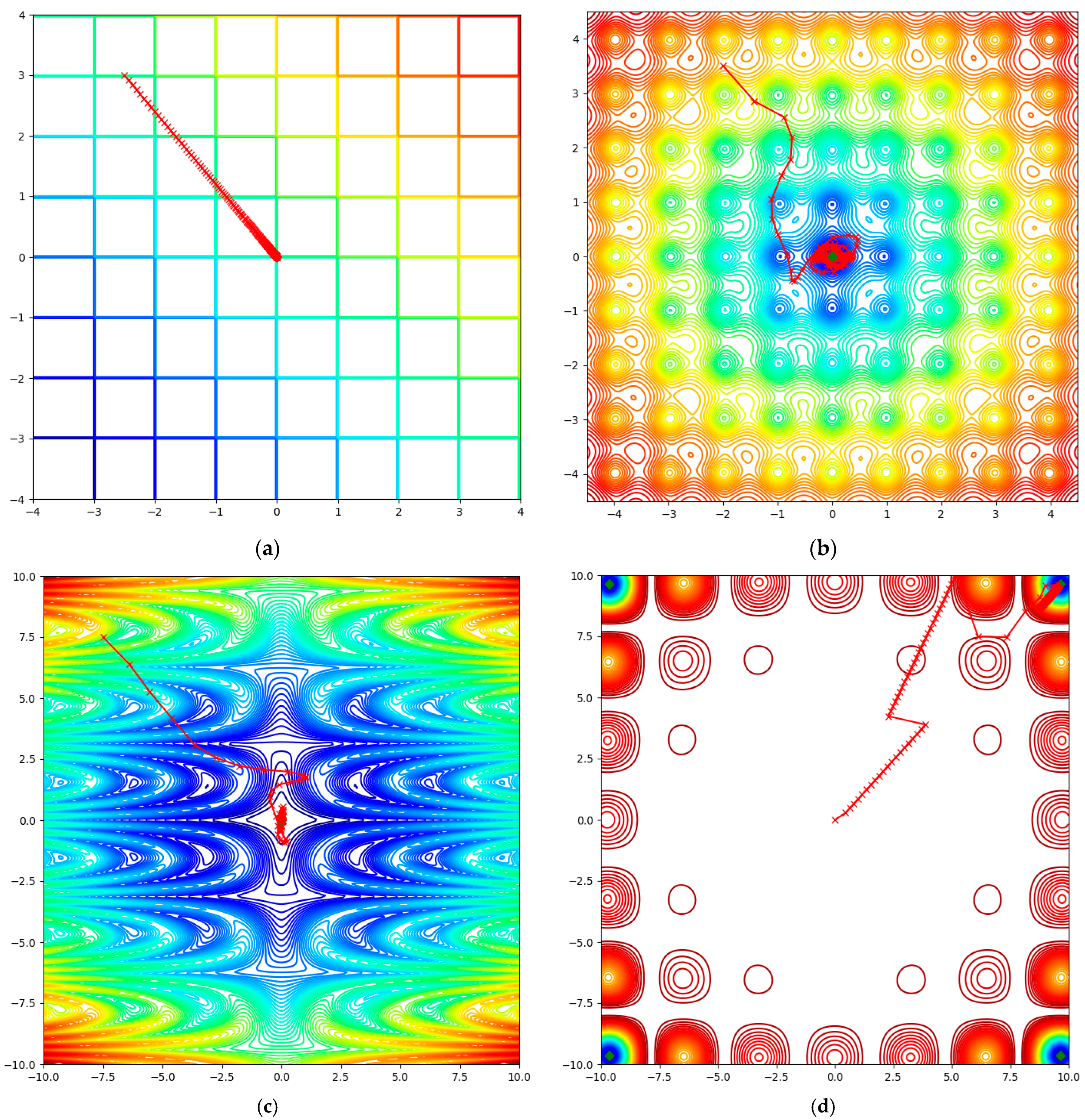
Before including the proposed YogiPNM and DiffPNM with coordinate descent in NNs, we examine the proposed optimization algorithms on test functions [35], such as Plateau, Ackley, Pinter, and Carrom. The Plateau and Carrom functions contain domains with vanishing gradient problems. The Ackley and Pinter functions have subsets with exploding gradient problems. We set the default parameter for each optimization algorithm. The maximal number of epochs is 500. The global minimums of the Plateau, Ackley, Pinter, and Carrom test functions are 0, −3.3068, 0, and −24.15, respectively. The corresponding initial points are (−2.5, 3), (−2, 3.5), (−7.5, −7.5), and (0, 0). In Figure 4, we show the minimization trajectory of the optimizer, which shows the smallest value compared to other approaches.

Considering the results in Figure 4 and

Table 1. Test function optimization by proposed and SOTA optimization algorithms.

Optimizer	Plateau	Ackley	Pinter	Carrom
SGD	3.00 × 100	1.58 × 10−1	4.68 × 10−2	9.89 × 100
AdamW	1.53 × 10−3	3.54 × 10−3	1.84 × 10−2	−2.21 × 101
AdaBelief	3.00 × 100	5.57 × 10−3	5.66 × 10−3	9.89 × 100
DiffGrad	3.00 × 100	8.40 × 10−4	2.85 × 10−3	9.89 × 100
Yogi	3.00 × 100	9.85 × 10−4	1.48 × 101	9.88 × 100
DiffPNM	6.47 × 10−4	3.05 × 10−4	3.16 × 10−3	−2.42 × 101
YogiPNM	8.36 × 10−4	2.89 × 10−4	2.01 × 10−3	−2.41 × 101

, we can infer that the proposed DiffPNM and YogiPNM with coordinate descent attain the global minimum of test functions, solving the vanishing and exploding gradient problems. We can see that the proposed DiffPNM and YogiPNM with coordinate descent give the best solutions for vanishing gradient and exploding gradient problems, respectively. Among SOTA optimizers, only AdamW considers the coordinate descent technique, unlike other known analogs.

The problem of vanishing and exploding gradients regularly occurs in the loss functions of modern NNs. Such issues are connected to drone detection problems, where night and far-distance conditions lead to exploding and vanishing gradient problems, respectively. For that reason, we suggest using a coordinate approach with gradient-based optimization. The proposed DiffPNM and YogiPNM with coordinate descent and SOTA approach AdamW attain the global minimum in the Plateau and Carrom test functions with a tiny gradient value, while other optimizers fail. In the case of exploding gradient, the proposed optimization algorithms demonstrate the smallest value of the Ackley and Pinter test functions. In the next subsection, we verify the quality of solving drone detection problems in visual datasets by Yolov11 and Yolov12 with the proposed optimizers.

5.2. UAV Detection in Video Data

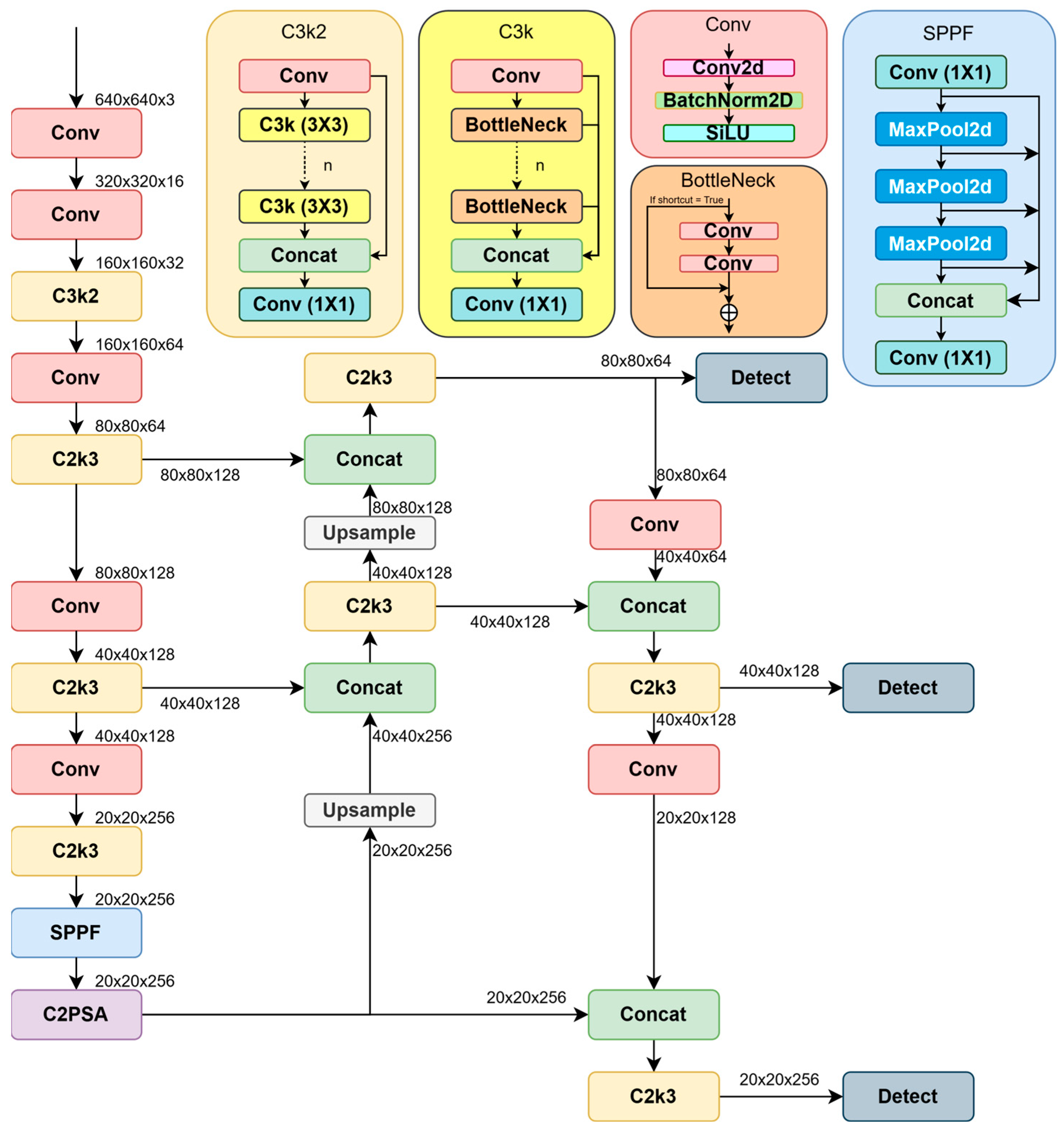
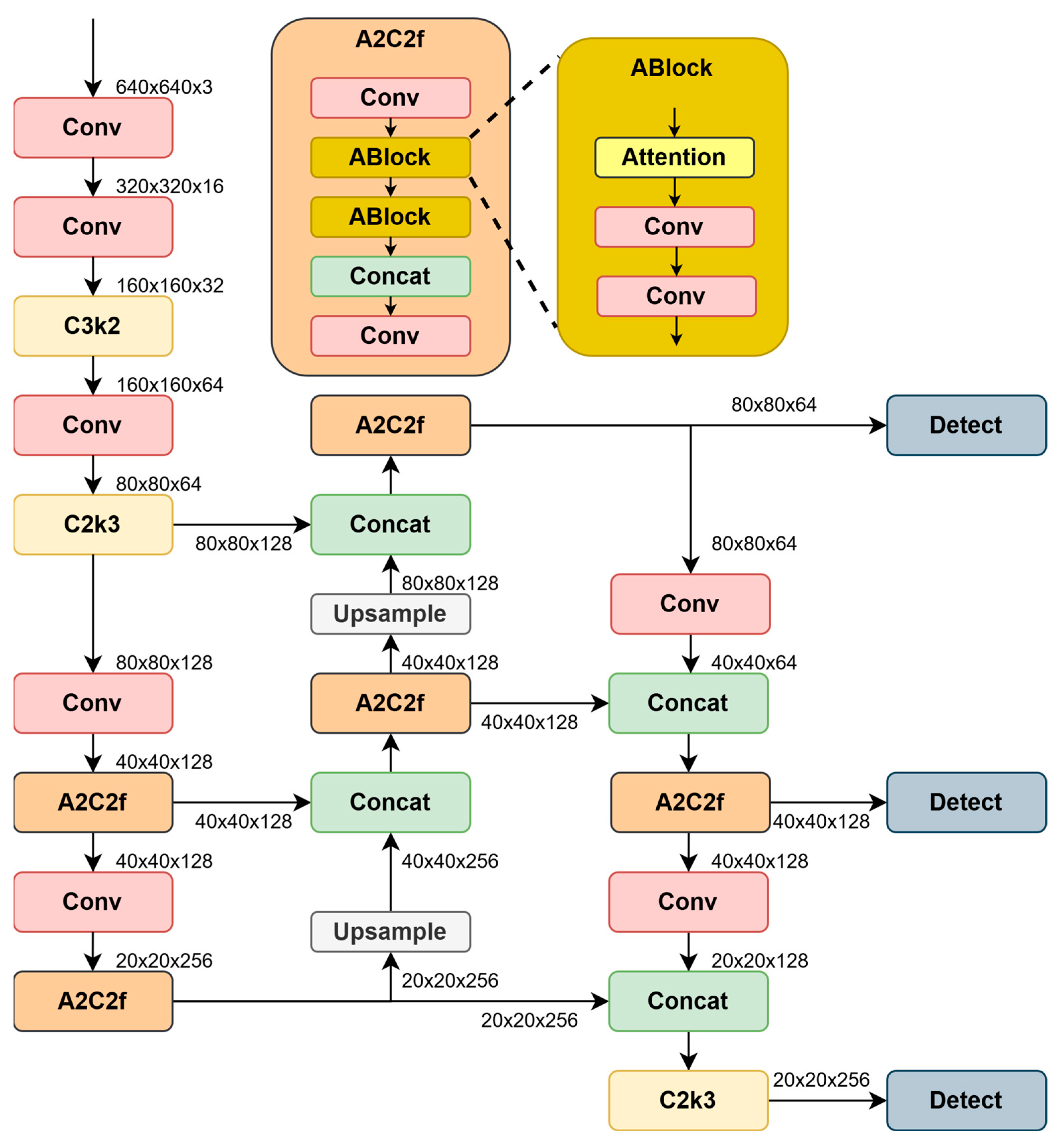
This section presents the experimental results obtained from the training process. The training is implemented on Yolov12 with positive–negative optimizers YogiPNM and DiffPNM. The open-source DroneDetectionDataset [36], which contains 51,446 RGB images in the test sample, was used in the training process. The provided videos are sufficient to evaluate NNs for solving the drone detection problem. Based on testing the developed deep learning model in the simulation environment, the most important shortcomings of the proposed NN can be identified so that the drone detection performance does not degrade in real-world conditions. Future research can implement the proposed architectures in real-world cases. All images have a resolution of 640 × 480 pixels. These images show drones in different types, scales, sizes, positions, environments, and times of day, with bounding boxes in XML format. Training of Yolov12 with the YogiPNM optimizer on the DroneDetectionDataset was conducted using the Kaggle cloud service. The experiment utilized a 16 GB NVIDIA Tesla P100 graphics card, PyTorch 2.4.0 deep learning library, Ultralytics 8.3.94 library, Python 3.10.14, CUDA 12.3, and Ubuntu 22.04.3 LTS 64-bit operating system. A loss function similar to Yolov8 was used for training. It can be represented by the following formula:

$$Loss=a\times {Loss}_{box}+b\times {Loss}_{dfl}+c\times {Loss}_{cls},$$

(8)

where Loss_box is the bounded box loss, Loss_dfl is the distribution focal loss, Loss_cls is the class loss, and a, b, and c are the weighting coefficients of the entries of each loss function into the overall function. In this experiment, a = 7.5, b = 1.5, and c = 0.5, respectively. These values are the default values used in the Ultralytics library and have been used by other researchers in training [14,37]. During training, the DroneDetectionDataset containing 51,446 images in the training sample and 5375 images in the validation sample was used. The test sample consisted of real drone flight videos taken from open sources and manually labeled using the CVAT tool. The size of the images fed to the NN input was 640 × 480, but all images were scaled to 640 × 640 before processing. This image resolution allows for real-time computation while still being able to recognize small objects. During the experiment, Yolov12 nano-models pre-trained on the COCO image set were additionally pre-trained for five epochs on the DroneDetectionDataset. Various optimizers, such as SGD, AdamW, AdaBelief, Yogi, DiffGrad, YogiPNM, and DiffPNM, were used for comparative analysis. All NN architectures were trained with the same hyperparameters presented in

Table 2. Important parameter settings.

Parameters	Setup
Epochs	5
Imgsize	640
Batch size	32
IoU	0.7
Initial Learning Rate	0.01
Final Learning Rate	0.01
Momentum	0.937
Warmup Epochs	3
Warmup Momentum	0.8
Mask ratio	4
Weight Decay	0.0005

.

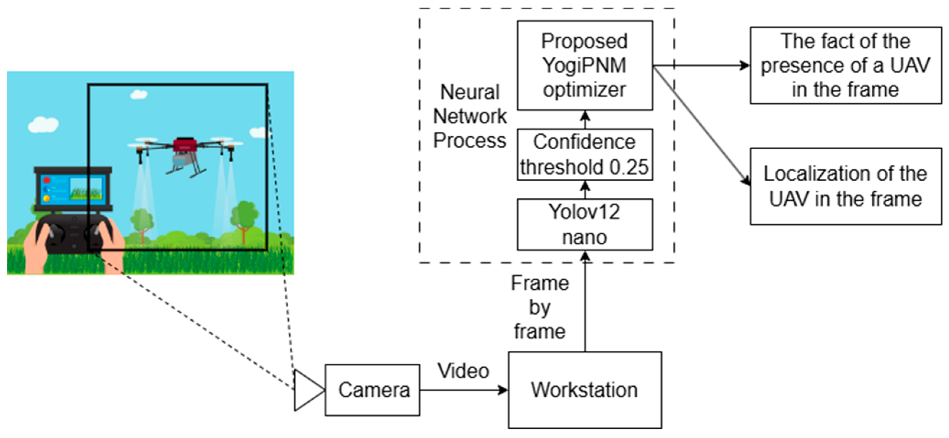
To determine the optimum value of the confidence threshold of the model, an experiment was conducted by testing NNs with different thresholds. The best threshold was determined by the values of the F1-score metric, as a metric combining precision and recall. The results are summarized in

Table 3. F1-score with different confidence thresholds for different optimizers.

Model	Optimizer	Confidence Threshold
		0.25	0.5	0.75
Yolov11	SGD	46.1	43.5	30.3
	AdamW	43.5	40.6	26.7
	AdaBelief	48.4	42.6	17.9
	DiffGrad	44.8	39.8	20.9
	Yogi	49.1	42.7	11.5
	DiffPNM	48.4	44.9	22.1
	YogiPNM	49.9	49.9	28.9
Yolov12	SGD	44.9	45.0	28.6
	AdamW	48	43.9	16.8
	AdaBelief	39.3	39.1	18.2
	DiffGrad	41.9	38.2	20.4
	Yogi	24.9	17.6	5.8
	DiffPNM	39.8	40.2	23.9
	YogiPNM	43.9	42.8	24.8

. In this table, the rows represent the name of the model and optimizer, the columns indicate the confidence threshold value, and the table fields show the F1-score value for this model at the specified confidence threshold. The model works best at a confidence threshold of 0.25. This value will be used in testing in all subsequent experiments.

The metrics precision, recall, mean average precision (mAP) 50, and F1-score were chosen to evaluate the performance of the NN. Precision and recall are calculated using the following formulas:

$$Precision={\displaystyle \frac{TP}{TP+FP}}\times 100\%,$$

(9)

$$Recall={\displaystyle \frac{TP}{TP+FN}}\times 100\%,$$

(10)

where TP (true positives) denotes the number of targets detected correctly, FN (false negatives) is the number of targets detected as backgrounds, and FP (false positives) denotes the number of backgrounds detected as targets. F1-score is a harmonic average between precision and recall. This metric provides a comprehensive assessment of the number of errors of the first and second kind. F1-score can be represented by the following formula:

$$F1Score={\displaystyle \frac{2\times Precision\times Recall}{Precision+Recall}},$$

(11)

mAP is a metric that allows the accuracy of localization of the object frame compared to the reference frame to be estimated. mAP50 means that the metric will be calculated considering only frames with an intersection over union (IoU) value greater than 0.5 (50%) to be correct. IoU and mAP are represented by the following formulas:

$$IoU\left(A,B\right)={\displaystyle \frac{A\cap B}{A\cup B}},$$

(12)

$$mAP=1/N\sum _{i=1}^N{AP}_i,$$

(13)

where A and B are the reference and predicted bounding boxes, N is the number of detectable classes, and ${AP}_i$ is the average accuracy of each category.

Experiments were conducted to train different combinations to determine the best combination of model and optimizers. A total of two architectures were chosen: Yolov11, as the state-of-the-art version of Yolo, based on CNN, and Yolov12, as the first architecture based on a self-attention mechanism. The following optimizers were chosen: SGD, AdamW, AdaBelief, DiffGrad, Yogi, YogiPNM, and DiffPNM [32]. The metrics precision, recall, mAP50, and F1 were chosen to evaluate the accuracy of model recognition. All metrics were computed from the results of processing two hand-marked videos of real drone flights. The images from these videos were not involved in the training and validation process. Simulation results from the first video are presented in

Table 4. Yolo simulation results from the first video with different optimizers.

Model	Optimizer	Precision (%)	Recall (%)	mAP50 (%)	F1-Score (%)
R-CNN	SGD	64.2	32.3	48.2	43.0
	AdamW	66.5	30.2	48.5	41.5
	AdaBelief	64.9	31.6	49.2	42.5
	DiffGrad	68.3	34.5	48.8	45.8
	Yogi	67.8	33.7	50.1	45.0
	DiffPNM	68.4	34.2	49.3	45.6
	YogiPNM	67.9	35.1	49.7	46.3
Yolov11	SGD	67.4	35.0	50.2	46.1
	AdamW	72.5	31.1	49.8	43.5
	AdaBelief	67.6	37.7	52.8	48.4
	DiffGrad	63.7	34.5	50.2	44.8
	Yogi	71.1	37.5	53.8	49.1
	DiffPNM	66.4	38.1	50.6	48.4
	YogiPNM	76.7	37.0	49.0	49.9
Yolov12	SGD	69.8	33.1	46.9	44.9
	AdamW	67.8	37.2	49.4	48.0
	AdaBelief	63.9	28.4	40.8	39.3
	DiffGrad	52.7	34.8	45.8	41.9
	Yogi	85.3	14.6	50.4	24.9
	DiffPNM	65.1	28.7	41.7	39.8
	YogiPNM	61.0	34.3	43.7	43.9

.

Looking at the results shown in Table 4, we can see that Yolov11 shows the best performance in recall (10), mAP50 (13), and F1-score (11). Among the Yolov11 models, the highest precision (9) and F1-score of 76.7% and 49.9% were obtained by training with the YogiPNM optimizer. AdamW and Yogi ranked second in these metrics, respectively. Training with DiffPNM improved recall by seven percentage points over the default AdamW. The Yolov12 architecture achieved the highest precision value when using the Yogi optimizer, but the value of the recall metric for this model is the lowest, indicating a high number of erroneous detections.

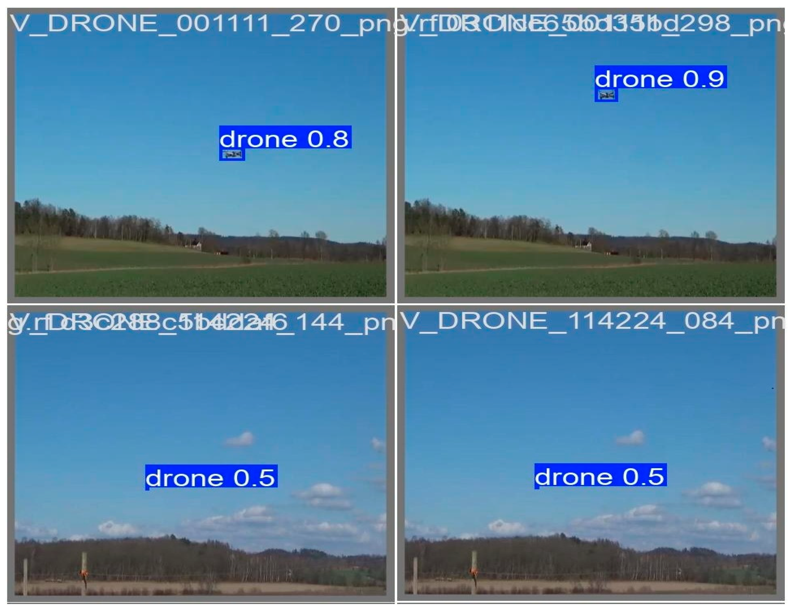
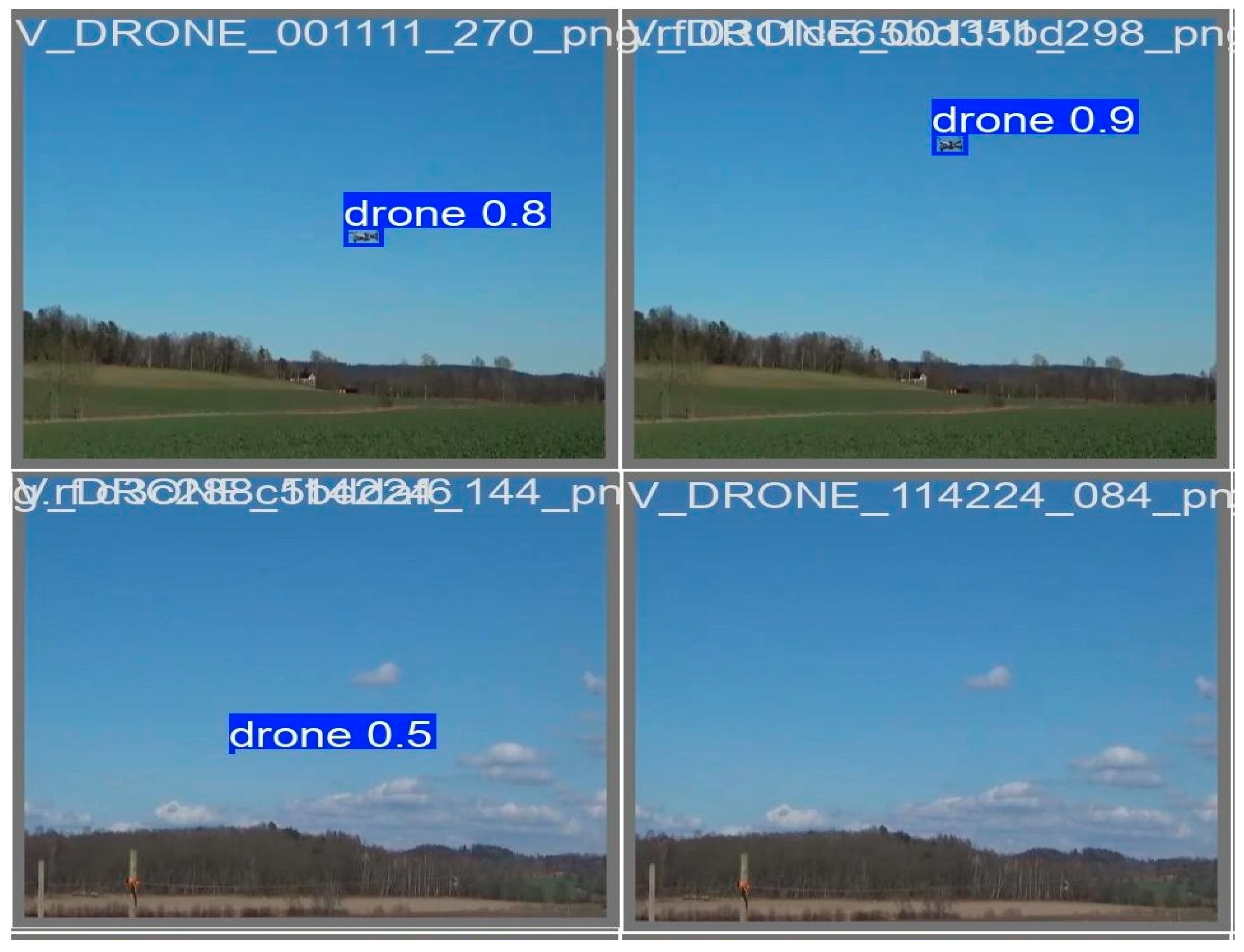
Figure 5 and Figure 6 show examples of image recognition using Yolov11 and Yolov12 with YogiPNM. These images show that Yolov11 fails to recognize a UAV against a dark background but recognizes a drone standing on the ground with a high degree of confidence. Yolov12 recognizes the drone against the background of trees.

Combining the information from Table 4 and Figure 5 and Figure 6, we can conclude that Yolov12 models create more frames and recognize the drone more often, but it also increases the number of false detections of other objects like UAVs. Yolov11 allows fewer erroneous detections, but it misses many frames with the presence of a drone without recognizing it. The results obtained from the processing of the second video are presented in

Table 5. Yolo simulation results from the second video with different optimizers.

Model	Optimizer	Precision (%)	Recall (%)	mAP50 (%)	F1-Score (%)
R-CNN	SGD	91.2	90.6	91.2	90.9
	AdamW	90.9	90.2	90.4	90.5
	AdaBelief	90.9	89.9	90.1	90.4
	DiffGrad	90.4	89.8	89.7	90.1
	Yogi	90.8	89.4	89.8	90.1
	DiffPNM	92.0	91.4	91.0	91.7
	YogiPNM	91.5	90.9	90.9	91.2
Yolov11	SGD	94.3	93.4	93.4	93.8
	AdamW	94.6	94.5	95.1	94.5
	AdaBelief	95.7	93.7	94.2	94.7
	DiffGrad	95.0	94.2	94.1	94.6
	Yogi	94.9	94.2	94.9	94.5
	DiffPNM	93.8	90.6	92.2	92.2
	YogiPNM	93.9	93.9	94.2	93.9
Yolov12	SGD	94.0	93.1	94.2	93.5
	AdamW	94.6	94.8	95.1	94.7
	AdaBelief	93.4	92.8	93.0	93.1
	DiffGrad	95.9	95.1	95.1	95.5
	Yogi	95.1	86.6	90.6	90.7
	DiffPNM	96.9	95.8	96.3	96.3
	YogiPNM	97.1	96.1	96.8	96.6

.

Analyzing the results presented in Table 5, we can conclude that the Yolov12 model with the YogiPNM optimizer was the best at processing the second video. The precision, recall, mAP50, and F1-score were 97.1%, 96.1%, 96.8%, and 96.6%, respectively. In second place is Yolov12 with DiffPNM. In third place is Yolov12 with the DiffGrad optimizer. Using the state-of-the-art optimization method improved precision by 3.1%, recall by 3%, mAP50 by 2.6%, and F1-score by 3.1 percentage points. For the Yolov11 model, the best optimizer was AdamW for recall and mAP50 metrics and AdaBelief for precision and F1-score. The NN based on the self-attention mechanism achieved a result that exceeded the best results of Yolov11 by 1.4–1.9 percentage points.

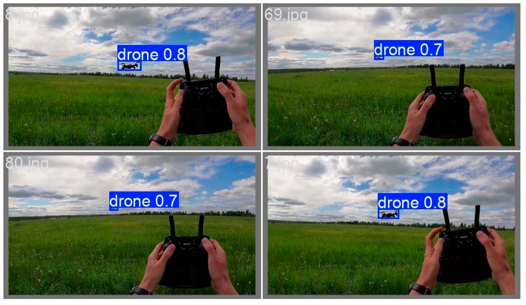
Comparing Figure 7 and Figure 8, it can be seen that both models perform well in recognizing the drone against a contrasting background. It can also be seen that Yolov11 shows more confidence in distinguishing the UAV in the bounding box.

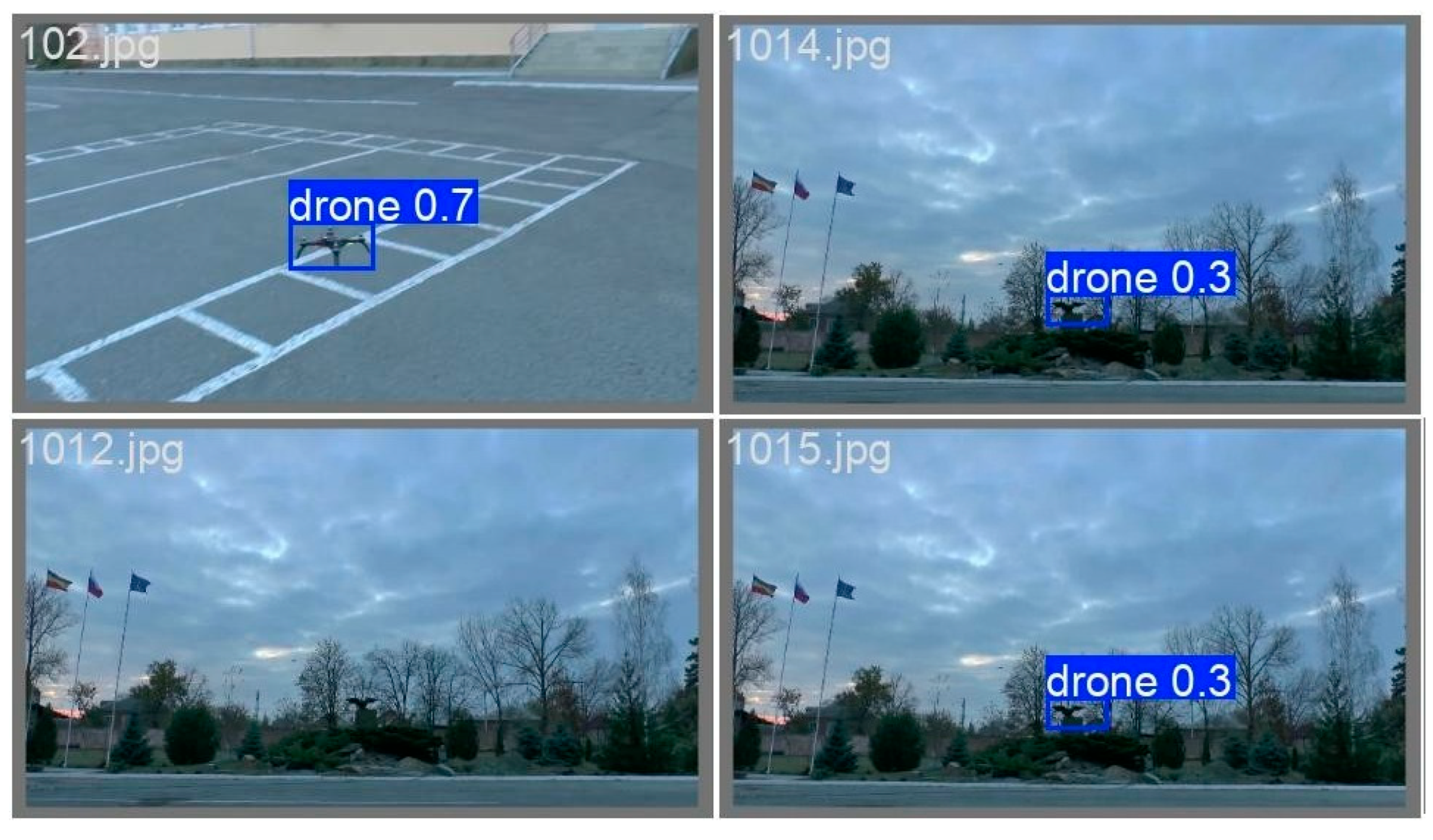
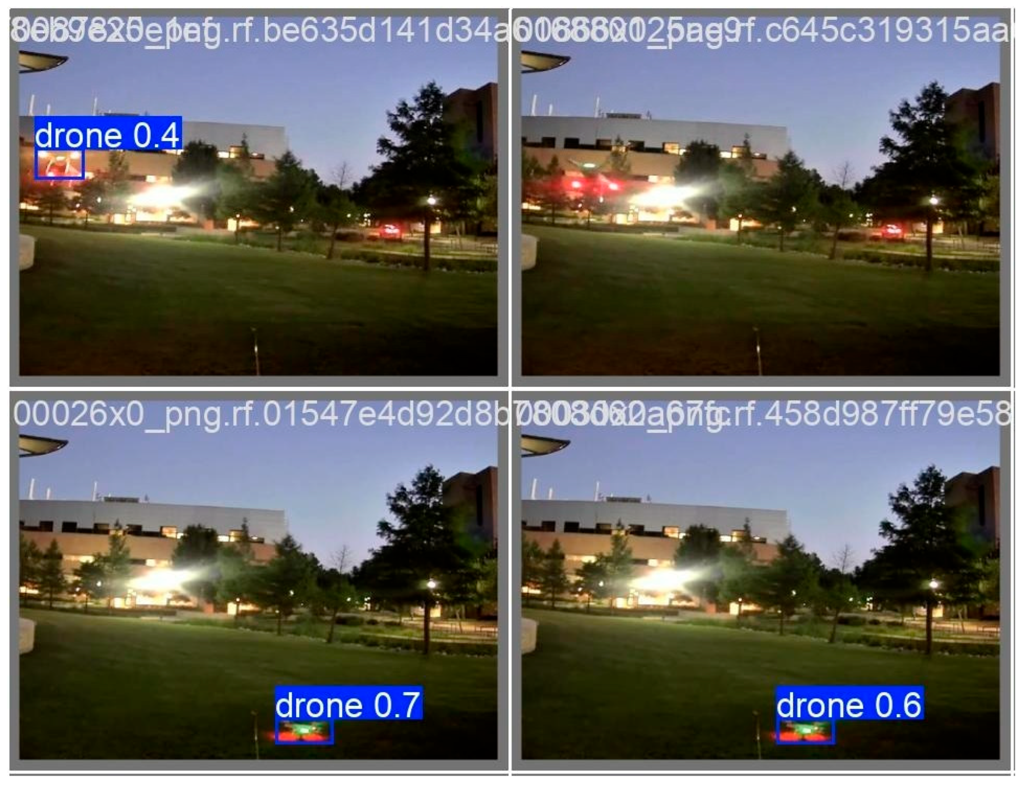
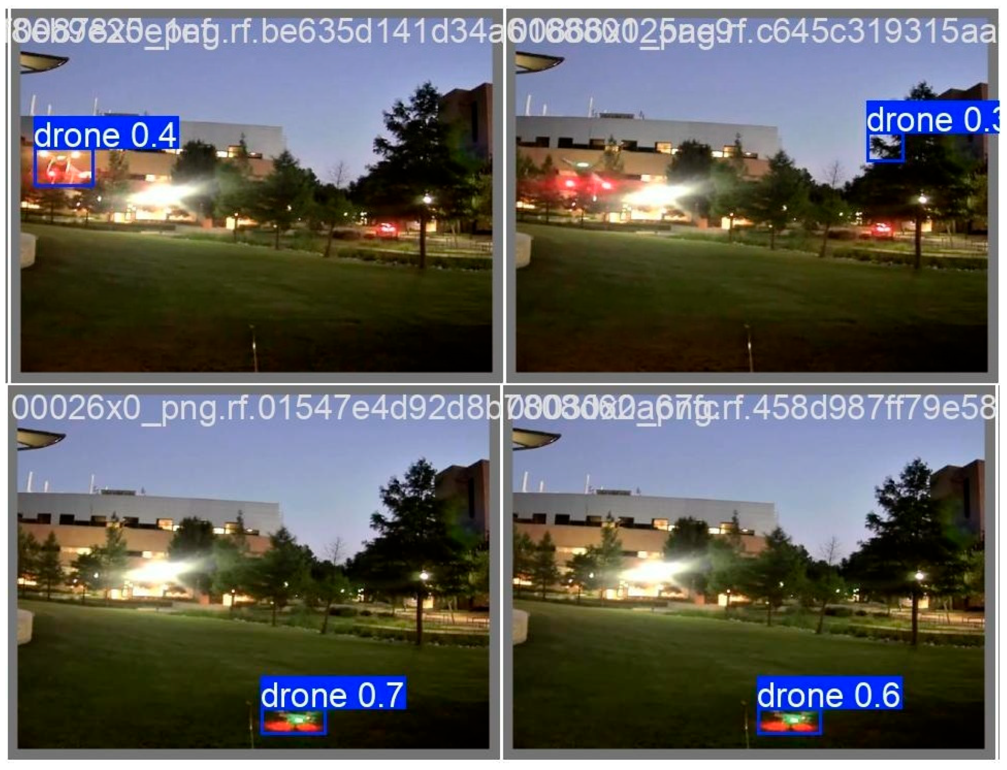
Additionally, we demonstrate the solving of the drone detection problem on night-time datasets. We show the results of drone detection and accuracy assessment in Figure 9 and Figure 10 and

Table 6. Image processing speed of Yolov11 and Yolov12 models in videos with night conditions.

Model	Optimizer	Precision (%)	Recall (%)	mAP50 (%)	F1-Score (%)
R-CNN	SGD	69.1	21.5	39.7	32.4
	AdamW	73.6	27.2	46.0	50.3
	AdaBelief	77.2	32.8	47.3	51.9
	DiffGrad	70.2	29.1	44.5	47.7
	Yogi	71.6	34.6	45.6	48.5
	DiffPNM	75.1	35.9	46.3	53.6
	YogiPNM	74.6	34.2	46.7	54.1
Yolov11	SGD	74.3	24.1	48.1	36.4
	AdamW	77.5	34.0	56.3	47.3
	AdaBelief	86.9	43.4	65.5	57.9
	DiffGrad	86.5	47.6	66.1	61.4
	Yogi	77.4	50.2	63.8	60.9
	DiffPNM	79.1	42.9	60.0	55.6
	YogiPNM	84.1	50.4	65.4	61.6
Yolov12	SGD	85.0	24.0	54.7	37.4
	AdamW	86.4	58.7	73.1	69.9
	AdaBelief	92.8	11.4	52.2	20.3
	DiffGrad	94.9	18.4	56.9	30.8
	Yogi	97.9	2.78	51.4	5.41
	DiffPNM	85.1	59.1	70.2	65.7
	YogiPNM	88.5	58.3	71.3	66.8

, respectively.

In the case of the R-CNN model, the proposed optimization algorithm DiffPNM demonstrates the highest quality of drone detection. YogiPNM gives the second-highest result in neural network training and drone detection. We can see that the proposed optimizers attain higher results than known analogs. In the case of Yolov11, the best average result belongs to YogiPNM. The optimizers DiffGrad and AdaBelief also demonstrate a high quality of drone detection problem-solving. Yolov12 attains the best results in solving the drone detection problem by using YogiPNM and DiffPNM approaches. The remaining SOTA optimizers either show lower-quality results or experience the anomalies in precision, recall, and F1-score.

Next, we examine our drone detection method in visual datasets containing far-distance conditions. We show the results of drone detection and accuracy assessment in Figure 11 and Figure 12 and

Table 7. Image processing speed of Yolov11 and Yolov12 models in videos with far-distance conditions.

Model	Optimizer	Precision (%)	Recall (%)	mAP50 (%)	F1-Score (%)
R-CNN	SGD	23.6	11.5	12.7	15.3
	AdamW	20.3	10.3	11.2	14.0
	AdaBelief	22.0	10.7	11.5	13.6
	DiffGrad	19.8	9.53	10.2	11.8
	Yogi	20.4	10.1	9.95	11.2
	DiffPNM	24.2	13.1	11.8	13.5
	YogiPNM	23.8	12.7	11.3	14.0
Yolov11	SGD	28.6	13.2	14.0	18.1
	AdamW	24.7	12.4	14.1	16.5
	AdaBelief	26.2	11.1	12.9	15.6
	DiffGrad	22.3	11.8	13.3	15.4
	Yogi	26.6	12.1	14.1	16.6
	DiffPNM	26.4	12.7	14.2	14.5
	YogiPNM	26.9	13.0	14.2	15.6
Yolov12	SGD	31.2	13.0	15.8	18.9
	AdamW	28.3	12.4	14.6	17.2
	AdaBelief	25.4	11.3	13.4	15.7
	DiffGrad	23.7	11.8	13.4	15.6
	Yogi	30.4	9.93	19.0	14.0
	DiffPNM	29.1	13.1	15.3	14.5
	YogiPNM	28.9	12.7	14.6	14.1

, respectively.

In the case of the R-CNN model, the proposed DiffPNM demonstrates the highest average result of drone detection. YogiPNM gives the second-best drone detection quality results. Among SOTA optimizers, SGD shows the best results in solving the drone detection problem. We can see that the proposed optimizers attain higher results than known analogs. In the case of Yolov11, the best average result belongs to YogiPNM. The optimizers DiffGrad and AdaBelief also demonstrate a high quality of drone detection problem-solving. Yolov12 attains the best results in solving the drone detection problem by using YogiPNM and DiffPNM approaches. The remaining SOTA optimizers either show lower-quality results or experience the anomalies in precision, recall, and F1-score.

The main advantage of the Yolo architecture over other architectures for solving the detection problem is the ability to work in real time. Yolov12 has five architecture sizes: nano, small, medium, large, and extra-large.

Table 8. Image processing speed of Yolov11 and Yolov12 models.

Model	Size	Params (M)	FPS
Yolov11	Nano	2.6	160.96
	Small	9.4	147.52
	Medium	20.1	97.12
	Large	25.3	84.00
	Extra-large	56.9	49.12
Yolov12	Nano	2.6	152.26
	Small	9.3	141.98
	Medium	20.2	88.48
	Large	26.4	64.96
	Extra-large	59.1	39.20

was constructed to evaluate the feasibility of using larger architectures for real-time image processing. It shows the model name, size, number of parameters, and FPS.

Thus, for real-time video processing at 60 fps, all models except extra-large can be used. The proposed Yolov12 model achieves high performance in the task of UAV recognition in the video stream; however, the result can be improved by using larger Yolo models such as Yolov12s, Yolov12m, or Yolov12l. The peculiarity of the proposed models Yolov11 and Yolov12 is the use of optimization algorithms with positive–negative momentum estimation and coordinate descent. Unlike models using optimization of SOTA algorithms, our development achieves high accuracy of object detection in fewer epochs, and as a result, the occurrence of overfitting for calculating convergence on a global scale with minimal feature loss.

6. Discussion

Based on the results presented in Table 4, Table 5, Table 6 and Table 7, we can conclude that using Yolov11 and Yolov12 with YogiPNM and DiffPNM improves recall and F1-score for the UAV recognition task.

Table 9. Evolution of neural networks for solving object detection problems.

Neural Network	Key Idea	Year
R-CNN [9]	Detection of objects based on regions	2014
SSD [23]	Single-stage detection with Anchor Boxes	2016
RetinaNet [24]	Feature pyramid network and focal loss	2017
EfficientDet [25]	EfficientNet backbone with bidirectional feature pyramid network	2020
Yolov11 [15]	Combining class prediction and object localization into a single process	2024
Yolov12 [16]	Integration of attention mechanisms without compromising work time	2025
Proposed Yolov12 with YogiPNM	Yogi positive–negative momentum optimizer	2025

presents the chronology of the development of NN architectures used for the detection task.

In this paper, we propose the method of solving the drone detection problem via advanced Yolov-type neural networks and proposed positive–negative momentum optimizers, considering the coordinate descent technique. Such optimization algorithms attain the global minimum of the loss function (8). We examined the proposed optimizers on the Plateau, Ackley, Pinter, and Carrom test functions, which contain vanishing and exploding gradient problems. The proposed optimizers solve the corresponding optimization problem, regularly meeting in object detection. This advantage lets Yolov11 and Yolov12 detect drones in videos containing normal, night, and far-distance conditions with higher accuracy than other SOTA optimizers. Moreover, the convergence rate of YogiPNM and DiffPNM with the coordinate descent technique satisfies the conventional O(√T) estimation in modern neural networks. However, the proposed optimizers, like the provided SOTA approaches, analyze the loss function by gradient directions and moments. The gradient structure is not adaptive under loss function minimization problems, such as indefinite area avoidance and global minimum search in noisy domains. The application of zero-order and second-order optimizers is not suitable for solving these problems because of insufficient loss function analysis. As a solution, it is possible to use tools from fractional calculus and information geometry, which transform the gradient structure into a more adaptive version and measure the difference between data via divergences, respectively.

In paper [26], the authors show various drone detection methods: radio-frequency-based UAVs, visual data (image/video)-based UAVs, acoustic/sound-based UAVs, and radar-based UAV detection. Visual-based drone detection plays an important role in UAV flight trajectory planning, aerial surveillance, wildfire mapping, pipeline security, and environmental monitoring. This area of AI application experiences active growth and technological development, involving advanced NN models and optimization algorithms. Our method detects drones in visual datasets containing night and far-distance conditions. The proposed YogiPNM and DiffPNM with coordinate descent can be used in other neural networks, solving different problems in physics, industry, biology, chemistry, medicine, economics, and social sciences. The further possible modification of the proposed optimizers can include fractional gradient [38], defined via Riemann–Liouville, Caputo, or Grunwald–Letnikov derivatives. By transforming the usual gradient into a natural gradient via information geometry tools [39], one can improve the learning process via advanced divergences (Kullback–Leibler and Jennsen) and metrics (Wasserstein and Levy).

The advanced optimizers YogiPNM and DiffPNM increased the value of recall and F1-score metrics when detecting drones compared to SGD and AdamW. One of the known drawbacks is the deterioration of Yolov12 results when the distance to the drone increases. This problem can be attributed to the peculiarities of the architecture that utilizes the self-attention mechanism. The proposed model depends on the quality of video data and visibility conditions. This provides a basis for further development of NN models. Multimodal models that take into account other types of data in addition to visual data may increase the accuracy of UAV detection. For example, audio data [40] and radio frequency signals [41] can increase the distance and recognition accuracy by using more data.

7. Conclusions

During the experiments on test function minimization, we imply that the proposed optimization algorithms solve the problem of vanishing and exploding gradients. Our approaches attain the global extreme points, avoiding local minimums and passing through domains with large and tiny gradient values. Considering the results in Table 1, Table 2 and Table 3 and Figure 1, Figure 2, Figure 3, Figure 4 and Figure 5, we can see that Yolov11 and Yolov12 with the proposed positive–negative optimization algorithms, containing coordinate descent techniques, attain the highest quality of solving drone detection problems in normal, night, and far-distance conditions compared with SOTA approaches. In this paper, we demonstrated the impact of advanced optimization algorithms on the quality of solving drone detection problems on visual datasets containing night and far-distance conditions. Moreover, the proposed optimizers can be helpful in drone detection by radio frequency, acoustics, and radar datasets. By solving the problem of exploding and decaying gradients while minimizing the loss function, it becomes possible to implement the proposed models in solving real tasks, such as controlling the position of a drone in space or preventing collisions.

However, the proposed optimizer is the first-order approach, which significantly limits its potential. In further research, we can modify the proposed optimizers by integrating fractional-order derivatives [42], particle swarm optimizers [43], and Fisher’s information matrix [44]. Such a modification of the proposed optimization algorithms can increase the precision, recall, F1-score, and other metrics in object detection problem-solving. The additional utilization of modern schedulers [45] can improve the work of NN by the control of the learning rate update during the entire training process. Another important problem in solving drone detection is the increase in NN performance. Removing hidden blocks and layers results in a loss in drone detection quality. Therefore, one needs to use methods that preserve the NN structure. One of the most appropriate methods for improving the NN performance and minimizing loss in quality of drone detection is tensor decompositions of hidden layers [46]. All possible improvements can advance the existing machine learning models, which solve the drone detection problem on radio frequency, videos/images, acoustics, and radar analysis.