Abstract
Neural-network-based models have made considerable progress in many computer vision areas over recent years. However, many works have exposed their vulnerability to malicious input data manipulation—that is, to adversarial attacks. Although many recent works have thoroughly examined the adversarial robustness of classifiers, the robustness of Image Quality Assessment (IQA) methods remains understudied. This paper addresses this gap by proposing FM-GOAT (Frequency-Masked Gradient Orthogonalization Attack), a novel white box adversarial method tailored for no-reference IQA models. Using a novel gradient orthogonalization technique, FM-GOAT uniquely optimizes adversarial perturbations against multiple perceptual constraints to minimize visibility, moving beyond traditional -norm bounds. We evaluate FM-GOAT on seven state-of-the-art NR-IQA models across three image and video datasets, revealing significant vulnerability to the proposed attack. Furthermore, we examine the applicability of adversarial purification methods to the IQA task, as well as their efficiency in mitigating white box adversarial attacks. By studying the activations from models’ intermediate layers, we explore their behavioral patterns in adversarial scenarios and discover valuable insights that may lead to better adversarial detection.
1. Introduction
Image Quality Assessments (IQAs) are crucial to many computer vision tasks, such as image and video processing, content creation, and multimedia applications. By quantitatively measuring visual image and video quality, IQA metrics enable researchers, developers, and users to objectively evaluate the performance of image- and video-processing algorithms and systems. For example, traditional metrics such as the structural similarity index measure [1] (SSIM) and peak signal-to-noise ratio (PSNR), as well as more sophisticated learning-based approaches—e.g., LPIPS [2] and DISTS [3]—have seen wide use in assessing image compression and super-resolution performance. Furthermore, IQA models are widely used in other vision-related areas: examples include data filtration for processing large image datasets [4], compression quality optimization [5], ranking systems that include quality estimates as its component [6,7], and even quality-guided image generation with diffusion-based models [8]. The importance of IQAs has grown substantially due to the increasing volume of digital content created, transmitted, and consumed across various platforms.
IQA methods fall into two categories: full-reference (FR-IQA) and no-reference (NR-IQA). Full-reference models compare distorted images with their pristine references and evaluate visual differences between them, whereas no-reference models assess quality from a single image independently. This work focuses on NR-IQA, where neural networks have achieved remarkable accuracy but face underexplored risks from adversarial attacks. In this work, we use the terms “model” and “metric” interchangeably when referring to learning-based IQA methods.
The emergence of deep learning and neural networks has caused a shift toward machine-learning-based approaches for IQAs. Deep learning models, such as convolutional neural networks (CNNs) and Transformer-based architectures, have demonstrated a superior performance on a wide range of computer vision tasks, including IQAs. They can learn complex patterns and features from images, boosting accuracy and efficiency [2,9].
Despite their strong capability, neural networks have proven vulnerable to adversarial attacks [10]. Most common models, including CNNs and Transformer-based ones, are susceptible to manipulation through adversarial examples [11]—malicious input samples designed to deceive machine learning models and cause them to make incorrect predictions.
Adversarial attacks can compromise model performance and reliability, potentially creating security risks and safety concerns in real-world applications (Figure 1). To address this vulnerability of neural networks, researchers are exploring techniques and strategies to enhance robustness and resilience to threats. Adversarial training [12], defensive distillation [13], input preprocessing [14], adversarial purification [14], and many other approaches have been proposed to mitigate the impact of adversarial attacks.
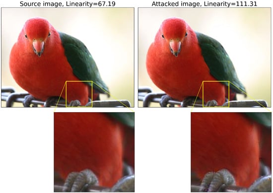
Figure 1.
Visualization of adversarial example crafted for Linearity [15] NR-IQA model using proposed adversarial attack. Predicted image quality almost doubled thanks to a visually imperceptible image perturbation. The source image is from KonIQ-10k database [16].
Adversarial attacks can manipulate IQA models’ outputs and distort the perceived visual quality of images, creating a threat to image-processing applications—such as image/video compression, enhancement, and restoration—where accurate quality assessment is essential. Exploiting a metric’s vulnerability in a compression algorithm, for instance, could yield inflated and biased scores during an objective evaluation. Furthermore, in some video compression codecs, quality metrics can directly influence the algorithm’s performance, as they explicitly optimize compression parameters to increase quality scores. One example, the AV1 video compression codec, offers the “tune=vmaf” and “tune=vmaf_neg” [5] preprocessing options specifically designed to boost results on the VMAF [17] video quality assessment (VQA) metric. Adversarially inflated quality scores might also misguide training loops [18] or enable the manipulation of quality-driven rankings.
Compounding this risk, IQA metrics themselves are increasingly used to evaluate the stealthiness of adversarial examples targeting other vision tasks [19,20]. Their ability to quantify perturbation visibility makes them both a tool for and a target of adversarial machine learning. Yet, the robustness of modern NR-IQA models under attack—their capacity to resist score manipulation—remains under-examined, thus making this research direction relevant for a more general research effort to evaluate and strengthen the robustness of image-processing neural networks.
The following list summarizes our contributions:
- A novel white box attack for NR-IQA. We introduce FM-GOAT, an adversarial method that goes beyond simple norm constraints in favor of multiple, differentiable human-vision-inspired metrics. It jointly optimizes against these constraints using a novel gradient correction technique, yielding imperceptible perturbations, extends seamlessly to video via motion-compensated propagation, and outperforms existing attacks in pair-wise comparisons across different NR-IQA models.
- Comprehensive vulnerability evaluation. We test six different NR-IQA architectures, demonstrating that all are highly susceptible to the proposed attack with a fairly limited perturbation budget.
- Deep feature analysis. By comparing intermediate model activations on clean and attacked inputs, we reveal characteristic patterns of perturbation propagation within different target models—insights that could inform more robust detection and defense strategies.
- Defense assessment. We benchmark common image transformations as purification defenses against the attack and show they only partially mitigate its effect, often introducing new artifacts that degrade model performance on benign images.
2. Related Work
2.1. No-Reference Image Quality Assessment
The no-reference Image Quality Assessment represents a well-established and actively evolving research domain that has gathered significant attention over the past decades, as it addresses the fundamental challenge of automatically evaluating the perceived quality of digital images without access to their pristine version. Early approaches focused on designing perceptual quality indicators through a statistical analysis of image properties, such as entropy differences in discrete cosine transform domains [21], high-boost filtering for local feature extraction [22], and natural scene statistics modeling [23]. These methods explicitly encoded principles of the human visual system, particularly sensitivity to high-frequency components and local texture variations. While effective for specific distortions and content types, their reliance on manual feature engineering limited their generalization across diverse quality assessment scenarios.
The advent of deep learning revolutionized NR-IQA through data-driven feature learning. Convolutional neural networks (CNNs) became predominant in the NR-IQA field, with architectures like those in Kang et al.’s foundational work [24] demonstrating end-to-end quality prediction from raw pixels. Subsequent innovations addressed dataset limitations with geometric augmentation strategies and hybrid training pipelines separating feature learning from quality score regression. Model designs were also continuously improving, building upon progressively more powerful backbones [25,26] and implementing effective architectural solutions: for instance, Ying et al. proposed a patch-based assessment approach [27], Su et al. adopted a hyper-network-based model for IQAs [28], and Li et al. introduced a novel loss design to improve training convergence [15]. The NR-IQA field further expanded beyond static images to video quality assessment (VQA), where temporal modeling techniques like recurrent networks [29,30] and efficient spatio-temporal sampling [31,32] emerged to handle motion artifacts and computational complexity.
Recent architectural advancements integrate attention mechanisms and Transformer-based designs to prioritize perceptually relevant regions, aligning predictions more closely with human judgments. Chen et al. implement a cross-scale attention mechanism in the TOPIQ model [33] to propagate multiscale features throughout the model, and Golestaneh et al. employ a Transformer encoder on image features in the TReS metric [34].
The field continues to evolve rapidly, with ongoing research exploring novel architectures, training methodologies, and evaluation protocols that push the boundaries of automated Image Quality Assessment capabilities. Current trends suggest a continued emphasis on leveraging foundation models for NR-IQA: recent works focus on assessing the applicability of Large Language Models, both open- [35,36] and closed-source [37], for the IQA task. The results emphasize the promising performance of large models that combine language and vision perspectives [35,38,39] in this domain; however, their applicability in resource-constrained environments remains a concern. Some of the most recent works further expand the field of quality assessment to a more general and sophisticated task of Image Quality Grounding [40,41], which focuses on generating detailed textual justifications for the quality score.
2.2. Adversarial Attacks
Adversarial attacks can be broadly categorized into two categories: (a) restricted methods, which generate an adversarial example by perturbing an image in a small -ball around it, and (b) unrestricted attacks, which synthesize new adversarial examples without limiting perturbation magnitude. Our work introduces a restricted attack but diverges from norm-based constraints, instead employing more complex differentiable functions that better reflect the concept of visual difference between images.
Adversarial attacks can be further classified by attacker knowledge [42]: (a) white box attacks assume full model access (including gradients with respect to inputs), and (b) a black box scenario assumes no prior knowledge about the target model, forcing the attacker to rely solely on input–output queries. Our focus in this work lies on iterative white box attacks.
The attacker’s goal can be either to achieve specific model outputs (a targeted attack) or to obtain any incorrect model response (an untargeted attack). Unlike classification, however, the IQA entails no unambiguous division of attacks in that regard. This paper considers an attack to be targeted if its goal is to change the output value in a certain direction (i.e., to increase or decrease it), and we only consider this scenario.
2.3. Restricted Attacks
Goodfellow et al. [10] introduced the Fast Gradient Sign Method (FGSM), one of the pioneering methods for adversarial example generation. It launched the research in this field and became a baseline for many subsequent works on adversarial attacks. The core idea of the attack is to perform one optimization step in the direction of the sign of the gradient calculated with respect to the input data. By taking the sign of the gradient, they accelerate the attack target’s growth when the gradient is small and simultaneously limit perturbation when the gradient is large; however, sign operation makes the optimization step rough and can introduce visible image distortions.
Since its inception, the FGSM has undergone multiple revisions. I-FGSM [43] was the first attempt to make the attack iterative, thereby reducing the size of each step and increasing its precision. MI-FGSM [44] extended this idea by adding momentum to the optimization. Shi et al. [45] proposed an iterative algorithm based on adaptive distortions. It employs the MI-FGSM attack along with the NIQE [46] quality metric to automatically infer the value of , limiting the attack in the norm. Madry et al. [47] introduced Projected Gradient Descent (PGD) to study the adversarial robustness of classifiers. PGD is functionally similar to I-FGSM but adds a random initialization in the allowed perturbation set (-ball). Many subsequent works further explored the field of iterative attacks for specific tasks, such as classification [48,49], object detection [50,51], depth estimation [52], IQAs [53,54,55], and others.
Moosavi-Dezfooli et al. [56] proposed a concept of Universal Adversarial Perturbations (UAPs): the attack’s goal is to generate a fixed perturbation, creating a high probability of deceiving the target model when added to an arbitrary image. Some approaches to crafting such perturbations involve interpolating adversarial additives generated for specific images [56] and training a CNN to generate UAPs [57].
2.4. Unrestricted Attacks
Although our work mostly focuses on restricted attacks, we also acknowledge recent progress in the field of unconstrained adversarial attacks. Since in this case the attacker is not limited to a small area around an existing data point, it enables many new sophisticated methods for generating adversarial examples either from scratch or from preexisting data. As the unlimited nature of unrestricted attacks indicates, however, the resulting adversarial examples are essentially new images that only resemble the original one, and usually the human eye can easily detect the difference in a pair-wise comparison. The visibility of such attacks and the “naturalness” of the resulting adversarial examples are noticeably difficult to control and objectively evaluate. Here, we describe only a few works to mark this field’s general research directions.
2.4.1. Generative Methods
Poursaeed et al. [57] proposed synthesizing adversarial examples through a specifically trained generative adversarial network (GAN) and thereby imitating a given data distribution while simultaneously disrupting the work of certain classifiers on synthesized images. Many subsequent works further developed this idea—most notably, Chen et al. [19] implemented an attack that uses recent progress in diffusion-based generative models [58]. It optimizes a latent representation of a benign input image so the output image, after several denoising diffusion steps, can fool the classifier, and it uses text guidance to retain the content and overall structure of the original image. Because diffusion models have just recently achieved astonishing image fidelity, they have yet to reach their potential in adversarial machine learning, and the possibility of their malicious use warrants recognition as well as a thorough examination.
2.4.2. Adversarial Texture and Color Correction
Bhattad et al. [59] offered two new approaches for unrestricted adversarial attacks against classifiers and image-captioning networks. The first one implements an adversarial colorization model that colors a grayscale source image with the help of color hints from the source image. It allows the preservation of vital structural information from the original image while introducing significant semantic modifications. The second approach applies the latest neural style transfer developments to manipulate the style of the benign image to better match that of certain target class examples.
2.4.3. Adversarial Deformations
Instead of manipulating images with additive noise or synthesizing new adversarial examples using generative models, adversarial deformation attacks create a geometric deformation of a benign image to fool the target neural network. Alaifari et al. [60] (ADef attack) and Xiao et al. [61] (StAdv attack) implement this idea by optimizing a vector field that warps the initial image. This approach moves source image pixels with their respective colors and thereby avoids producing new colors and noisy perturbations, but it also unnaturally distorts object shapes in certain cases, especially on low-resolution source images.
2.5. Adversarial Attacks on IQA Models
Various studies have examined the vulnerabilities of full-reference image- and video-quality metrics. Wang et al. [62] introduced the maximum differentiation competition (MADC) methodology to quality metric weaknesses by comparing, through subjective experiments, their performance on example image pairs that maximize or minimize one metric while keeping the other fixed. Ma et al. [63] extended this concept by creating group MADC (gMADC), which uses a group of models to generate adversarial images. Kettunen et al. [53] demonstrated the susceptibility of the learned perceptual image patch similarity metric [2] (LPIPS) to adversarial attacks using iterative optimization algorithms.
A few studies have also explored adversarial attacks on no-reference (NR) IQA models. Korhonen et al. [54] employed the Sobel filter and morphological operations to generate weight maps that limit the distortions to object edges. We use a similar idea in our work: reduce the attack’s visibility by masking the adversarial additive to high-frequency image regions. Zhang et al. [55] presented an iterative attack using different full-reference (FR) metrics to manipulate visual distortions. They chose an FR metric as the regularization term during optimization and found the optimal regularization strength by searching for the point of just noticeable difference (JND) through a subjective experiment. Shumitskaya et al. [64] researched the applicability of universal adversarial perturbation attacks to IQAs. The authors proposed several algorithms for training UAPs to attack NR-IQA metrics and a CNN-based method for adapting the pretrained universal perturbation to a specific image during inference. UAP-based methods are less computationally expensive than iterative approaches, but they lag in adversarial efficiency relative to iterative white box approaches.
3. Proposed Method
In this section, we present the Frequency-Masked Gradient Orthogonalization Attack (FM-GOAT) framework (Figure 2), a white box adversarial method that combines gradient optimization with perceptual constraints and high-frequency masking to manipulate NR-IQA models while minimizing perturbation visibility. First, we formulate the problem of adversarial attacks against NR-IQA models (Section 3.1), then we describe our multi-constraint gradient orthogonalization method (Section 3.2) and consider additional methods to further reduce the visibility of the adversarial perturbations both in images and videos (Section 3.3).
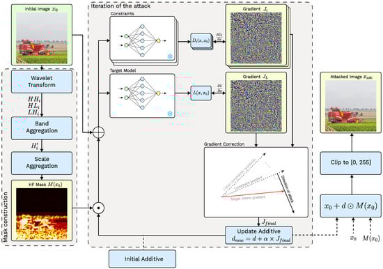
Figure 2.
Overall scheme of the proposed Frequency-Masked Gradient Orthogonalization Attack.
3.1. Problem Formulation and Constraints Design
We adopted the following general formulation of the adversarial attack against an NR-IQA model :
where X is an image space , L is a loss function corresponding to the discrepancy between the model’s output and expected output, and D measures perceptual distortion between the original image and adversarial example , bounded by threshold T.
In this work, we specify the attack goal as —that is, we set the attack direction to increase the target model’s output. We consider the increase in predicted image quality to be a more “practical” and dangerous use case in NR-IQA than decreasing the predicted quality or maximizing the difference between predictions. One of many possible examples is an image search engine that applies score-based ranking with an IQA metric as one of its components [6,7]; an attacker’s goal could be to raise his attacked image in the search results, encouraging him to increase the image’s predicted quality. Another common example of such attacks is cheating image/video-processing benchmarks (e.g., compression, super-resolution, or denoising). In this case, a contributor could inflate his algorithm’s evaluated performance by increasing the quality metric values through imperceptible adversarial perturbation.
Another important aspect of the attack is the choice of the constraint function D and its bound T. Many methods [10,43,47,62] suggest constraining the norm; doing so is justified by the ease of interpreting and enforcing such constraints, since one can simply clip the difference between images. However, this approach delivers suboptimal attack visibility, since , , and norms are known to correlate poorly with human perception of the difference between images [2,65]. Zhang et al. [55] address this issue by finding an optimal attack intensity through psychophysical experiments for each image individually, such that the adversarial example falls below the JND threshold. Our work intends to create a complete method that avoids the need for a subjective study to generate adversarial examples, rendering this approach inapplicable.
Instead, we focused on objective and differentiable constraint functions. Our method allows the use of an arbitrary number of such constraints——enabling the simultaneous consideration of multiple aspects of perceptual differences during the attack. A proper combination of several heterogeneous constraints also reduces the probability of inadvertently crafting an adversarial example for one of the constraint functions. Our experiments (see Section 4) employed the norm and SSIM [1] as low-level constraints and LPIPS [2] as a high-level visibility approximation.
3.2. Optimization Method
This section describes the proposed optimization method for solving the problem from Equation (1) with respect to the multiple differentiable constraints . It optimizes adversarial perturbations by aligning the target model’s gradient with the intersection of constraint function tangent spaces, thereby minimizing the collateral impact on the perceptual constraints. The core idea is to iteratively perform optimization steps that would both minimally affect the constraints and maximize the target model’s value. This is achieved through a modified Gram–Schmidt orthogonalization process [66] applied to gradient vectors.
Let (where ) denote the current adversarial image. Since for all functions are differentiable at the point , we compute gradients for the target loss and constraints :
The gradient points toward maximizing the target metric but may violate constraints. To preserve values, we project onto the intersection of the tangent hyperplanes orthogonal to each . This subspace is complementary to . Owing to the high dimensionality of the optimization space (the image’s pixel space) and the complex nature of constraint models, we can safely assume that their gradients form a linearly independent system. This implies that the subspace Q will have an orthogonal basis . Applying the Gram–Schmidt orthogonalization process to the gradients , we can iteratively construct this basis:
The corrected gradient orthogonal to constraint gradients therefore can be obtained from by subtracting its projection on orthogonal basis of Q:
yielding a perturbation direction that maximizes all while minimizing the collateral effect on the constraints . We can then update the adversarial additive d and adversarial example with a step size as follows:
In a strict mathematical sense, even a sufficiently small step in the direction orthogonal to the gradients of all constraint functions may go outside their level set thanks to high non-smoothness and the complexity of neural networks, yet it still appears to be an efficient approximation of the constraint-preserving optimization step. We further explore the effects of gradient correction on the resulting gradient’s magnitude and direction in Section 5.1.
We use the original image as the initialization of (i.e., we initialized the attack additive d with zeros, which we then add to the image ) because it allows us to guarantee minimal values of the distance functions at the initial optimization moment, whereas random initialization may immediately force beyond acceptable limits. When using such initialization, the functions that specify the distance to will begin with zero value and gradients so the first iteration does not subtract projections, thereby avoiding division by zero in the operation.
Unlike Lagrangian methods, which combine objectives and constraints via a tunable parameter :
the proposed method requires no additional hyperparameter tuning, except for the step size (a common requirement for all methods).
To better demonstrate the concept, we compare the proposed gradient correction approach with other optimization methods on a simple two-dimensional example. The objective is to optimize one function while preserving the other. Figure 3 demonstrates the setup. It can be seen that the trajectory directions produced by the proposed method align well with the level sets of the constraint function. The gradient correction approach effectively converges to a local minimum and maintains constraint adherence more reliably than -dependent relaxation, which struggles to balance competing objectives without careful calibration.
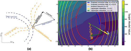
Figure 3.
(a) Visualization of a gradient correction step in a simple single-constraint case. In practice, orthogonality to multiple constraint gradients is maintained during the attack. (b) Visual comparison of optimization techniques on the toy 2D example. The color gradient depicts the target function, and the level lines depict a single constraint function. Dotted lines represent trajectories of different optimization methods.
3.3. Reducing Attack Visibility
This section first describes a wavelet-based masking that conceals adversarial perturbations in images and then introduces the propagation algorithm to transfer the FM-GOAT attack to the video domain while minimizing the severity of temporal artifacts.
3.3.1. High-Frequency Masking
Gradient-based attacks often produce adversarial perturbations that introduce noticeable high-frequency noise in the attacked image. This effect is due to the increased sensitivity of neural networks to manipulations of high-frequency information embedded into the image [67]. The human visual system, conversely, is more sensitive to low-frequency semantic information and hardly notices minor high-frequency changes to information-rich image regions. In information-poor regions, however, noise becomes apparent. Leveraging this discrepancy, we augment the attack with an additional masking stage that concentrates adversarial perturbations in inherently high-frequency regions (e.g., edges and textures), as illustrated in Figure 4.
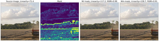
Figure 4.
The effect of incorporating our high-frequency masking method into the adversarial attack. Adversarial perturbations disappear from low-frequency regions (e.g., sky and clouds) and concentrate in high-frequency regions (e.g., tree crowns on the horizon).
In order to construct the high-frequency mask, we first apply the Discrete Wavelet Transform (DWT) to decompose the input image into low-frequency (L) and high-frequency () bands:
Each tensor in this decomposition contains the bands for different image scales. The number of high-frequency tensors depends on the DWT parameters. Our experiments used .
Next, we aggregate the bands for each image scale: first, we rescale the tensors to the input image resolution in the last two dimensions, then sum them over all channels, and clip to the range, thus obtaining :
where clips all elements of X to range , and rescales X to the required size using bicubic interpolation. Finally, to combine maps from different image scales, we sum the absolute values of and clip them again to . Lastly, we apply Gaussian blur with to the resulting mask as an additional post-processing step to reduce its overall sharpness:
where denotes the element-wise absolute value, denotes Gaussian blur, and is the desired mask.
The mask is computed only once for an input image and remains fixed during the optimization to prevent introducing artificial high-frequency content in the low-frequency regions of the original image. Adversarial perturbations are then applied as
where ⊙ denotes element-wise multiplication. This ensures that adversarial noise aligns with existing high-frequency structures, enhancing imperceptibility.
3.3.2. Propagating Adversarial Attacks on Videos
Extending image-based attacks to videos requires addressing computational efficiency and temporal consistency. While naively attacking each frame independently efficiently inflates the target model’s scores, this approach is prohibitively expensive and introduces noticeable flickering artifacts due to inconsistent perturbations across frames. Instead, we aim to make the adversarial perturbation change continuously from one frame to another. Our approach propagates perturbations from sparsely attacked keyframes to neighboring frames using motion compensation and interpolation, therefore leveraging significant structural overlap in neighboring frames. The overall workflow of the proposed propagation method is summarized in Figure 5.
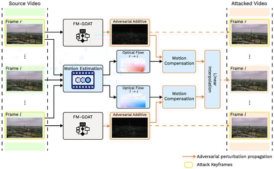
Figure 5.
Overall scheme of the proposed video propagation method.
First, we uniformly sample n frames (including start/end frames) from the source video and compute their adversarial perturbations using the image-based FM-GOAT algorithm. Next, for each intermediate frame , we identify the two nearest keyframes and () and calculate motion vectors between and these keyframes using the block-based motion estimation [68] algorithm:
The block-based motion estimation algorithm helps preserve local patterns in adversarial perturbations within each block while transferring them between frames. It also imposes only a small computational load compared to pixel-wise approaches and is reasonably accurate. As it only transfers adversarial additives without affecting the contents of the frames, motion vectors do not require remarkable precision.
Next, keyframe adversarial perturbations and are warped to align with using the motion compensation algorithm:
Finally, we blend warped perturbations and using linear interpolation based on the temporal proximity of the corresponding keyframes:
This interpolation strategy ensures smooth perturbation transitions while maintaining attack efficacy. Empirical tests show that the attacking additive retains its effectiveness only on the nearest neighboring frames in a small temporal interval, even for rather non-intensive scenes (see Figure 6). Therefore, interpolating between two neighboring keyframes instead of just the previous one also increases the average efficiency of the interpolated adversarial additive.
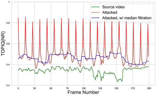
Figure 6.
Visualization of TOPIQ(NR) scores before and after attack on the “Aspen” video sequence from the Derf dataset. Attacked score peaks correspond to independently attacked frames. Performance of the adversarial additive drops even for neighboring frames. The blue line shows attacked scores after median filtration with kernel size 11.
4. Experiments
4.1. Experimental Setup
We chose the NIPS2017 from the NeurIPS Adversarial Vision Challenge [69] as a primary evaluation dataset, as it often serves as a benchmark for adversarial attacks on classifiers. NIPS2017 includes a subset of 1000 images from ImageNet, all of which are of resolution. We have also utilized the KonIQ-10k IQA dataset [16] and Derf video collection [70] for additional experiments. KonIQ-10k consists of 10,073 images of resolution , and Derf contains 24 short FullHD videos.
We evaluated the robustness of seven neural-network-based NR-IQA models, namely:
- PaQ-2-PiQ [27]: CNN-based NR metric that predicts image quality by analyzing patches and pooling them in accordance with regions of interest (RoI Pooling) to assess the quality of the entire image. It underwent training on the eponymous PaQ-2-PiQ subjective-quality database and uses ResNet-18 as a feature-extraction backbone.
- Linearity [15]: A model that introduces a novel norm-in-norm loss for NR-IQA training, demonstrating up to faster convergence than traditional loss functions such as MAE and MSE. It is based on a ResNeXt-101 backbone.
- Hyper-IQA [28]: An IQA metric specifically designed for real-life images, utilizing a hyper convolutional network to predict weights for the last fully connected layers. Feature extraction is performed by using the ResNet-50 backbone.
- TReS [34]: A metric that incorporates a self-attention mechanism for computing nonlocal image features as well as a CNN (ResNet-50) for extracting local features. It also introduces a self-supervision loss calculated on reference and flipped images.
- MDTVSFA [30]: An improved version of the VSFA video quality assessment metric. It employs a ResNet-50 backbone for feature extraction and a GRU recurrent network for temporal feature aggregation. MDTVSFA enhances VSFA through multi-dataset training and a score mapping technique between predicted and dataset-specific ground-truth quality scores. According to benchmark [71], it delivers a state-of-the-art VQA performance. It handles images as well by treating them as one-frame videos.
- TOPIQ(NR) [33]: A no-reference version of the novel TOPIQ metric, which introduces the coarse-to-fine network (CFANet) to employ multiscale image features and effectively propagate semantic information to lower-level features. It is among the top-performing IQA models in terms of computational efficiency and correlation with subjective quality.
- CLIPIQA+ [39]: CLIPIQA+ is a popular metric that employs a pretrained Vision–Language model for NR-IQA. It utilizes pairs of positive and negative text prompts to assess different aspects of image quality and further adopts the CLIP model [72] to the IQA domain using trainable context tokens. It also utilizes the ViT [73] backbone in its vision branch.
To objectively evaluate perceptual losses, our experiments used four FR metrics: the SSIM [1], a classical nonparametric method that captures structural information losses; LPIPS [2], a popular neural-network-based FR metric that assesses the perceptual difference between images by comparing features from deep layers of its CNN backbone; and PieAPP [74] as well as DISTS [3], common learning-based metrics that demonstrate good correlation with subjective quality. LPIPS is widely used in many computer vision domains, both as a part of a loss function for image restoration tasks and for evaluation. DISTS is robust to texture variance and slight geometric transformations, and PieAPP shows promising results in super-resolution-quality assessments [75].
4.2. Comparison with Other Attacks
We benchmark FM-GOAT against two NR-IQA-specific iterative attacks, Korhonen et al. [54] and Zhang et al. [55], and two classification-derived methods: I-FGSM [10] (a restricted attack akin to PGD without randomization) and StAdv [61] (an unrestricted geometric attack that optimizes spatial transformations). I-FGSM is a classic method widely used in the adversarial robustness field, and StAdv represents the class of unrestricted attacks: it generates examples that diverge least from the original images compared with other unrestricted attacks, both visually and according to objective FR metrics.
For all attacks, we fixed the number of iterations at five. For Korhonen et al. and Zhang et al., we use the default learning rate of , and for I-FGSM, we use . For StAdv, we set the learning rate at and and parameters at 50 and , respectively. These parameters specify roughly similar adversarial efficiencies among the attacks in our comparison. For all attacks, target metric outputs were normalized to the closest magnitude of 10 for cross-model consistency, since for many neural-network-based metrics, their ranges are not strictly defined. Implementations of all compared attacks, including FM-GOAT, are available at https://github.com/X1716/FM-GOAT (accessed on 9 June 2025). For FM-GOAT, we chose the (MSE), the SSIM, and LPIPS as gradient-correction constraints. All attacks start with zero-initialized additive (flow vectors in the case of StAdv) and are therefore deterministic. Computational performance evaluations of all tested attacks can be found in Appendix B Table A1 and Table A2. Figure 7 visually compares the adversarial examples generated with different attacks.
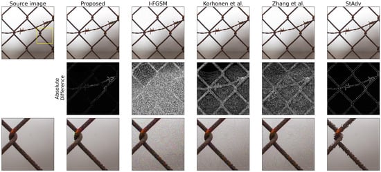
Figure 7.
Visualization of adversarial examples generated using different attack methods. First row depicts the adversarial examples, second visualizes the absolute difference with the source image, and the last demonstrates zoomed regions from the corresponding images.
Different attacks have different sets of parameters, and these parameters affect the gains of the target metric and the collateral perceptual losses unevenly. We implemented the following strategy to account for these differences and ensure a fair comparison.
To compare different adversarial attacks, we consider two core performance metrics that measure the attack’s efficacy from two opposite perspectives: adversarial efficiency and visual losses. Adversarial efficiency captures the attack’s effect on the target model: for NR-IQA, we define it as the gain in the target model’s output values. Visual losses represent the perceptual difference between the original image and its adversarial counterpart. Both of these statistics depend on the attack’s strength parameters and therefore should be evaluated independently.
To independently compare adversarial gains and visual losses, in the following two experiments, we fix one of the factors on a similar level and then compare the other one. As it is non-trivial to jointly align the statistics of multiple attacks, we conduct the comparisons in a pair-wise manner: for each test image, we fix one of the factors (adversarial gain or visual losses) on the level achieved by the competing attack, and then tune the hyperparameter of FM-GOAT to reach the same value for this factor. Then, we compare the opposite statistic between the two attacks. We use logarithmic range and 50 iterations per image for the parameter search. If an exact match was not found, we use the closest value erring on the side of a worse value for FM-GOAT as a conservative approximation.
4.2.1. Comparison Under Fixed Gains
Evaluation method. To equalize adversarial gains between FM-GOAT and other attacks, we gradually increase our attack’s parameter (boosting its strength and therefore the target metric’s gain) until the target metric’s increase from our attack becomes greater than or equal to that from the competing attack. We perform this procedure for each dataset image and each attack in the comparison. Next, we compare the values of FR metrics that approximate perceptual losses and calculate the “Win Rate”: the percentage of cases for which the losses due to our attack were less than those due to the competing attack for each FR metric:
where D is a distance FR-IQA metric, is a benign image, and and denote its adversarial counterparts produced by FM-GOAT and the competing attack, correspondingly. Higher Win Rate values (over 50%) indicate that FM-GOAT manages to achieve equal adversarial efficiency to the competing attack, all while resulting in lower perceptual losses, as measured by the distance function D.
Table 1 presents the results of this comparison.

Table 1.
Pair-wise perceptibility comparison of the FM-GOAT with other adversarial attacks (identified in top row) measured with Win Rate (↑) under equal adversarial efficiency. Win Rate is defined as the percentage of cases where FM-GOAT yields lower perceptual losses, measured using a given FR metric (identified in the second row), while achieving equal or higher adversarial gain of the target model (defined in first column). Note that 50% represents a tie.
In most scenarios, FM-GOAT consistently outperforms other methods, reaching the same adversarial efficiency while being preferred by multiple objective perceptual loss estimates. For I-FGSM and StAdv attacks, lower visual losses are achieved in almost every case. The only exception is the DISTS FR-IQA metric and the Zhang et al. attack, as the former includes direct DISTS optimization in its loss function, thereby improving its performance when undergoing evaluation by DISTS, suggesting that it might have also been compromised during the attack, along with the target NR-IQA model.
4.2.2. Comparison Under Fixed Perceptual Losses
Evaluation method. To compare the attacks under a fixed level of visual losses, we follow a similar approach: for each image, FM-GOAT uses the maximum value that still produces an adversarial example with perceptual losses less than or equal to those of competing attacks in a pair-wise comparison. Then, to compare the adversarial efficiency of the attacks, we measure the difference in the target model’s quality scores for adversarial examples produced by these attacks relative to the initial quality score:
where is a target NR-IQA model, is a benign image, and and are corresponding adversarial examples. Positive values of this metric indicate that FM-GOAT inflated the target model values more efficiently than the competing attack, and near-zero values represent an equal performance between the two attacks. This setup allows us to compare the adversarial efficiency of FM-GOAT with other attacks within an equal perturbation budget, all while using effective FR-IQA models as distance functions instead of -norms.
Table 2 presents the average relative gains for the NIPS2017 dataset, using the SSIM, LPIPS, DISTS, and PieAPP FR metrics to equalize perceptual losses. Our attack achieves a higher adversarial efficiency than the competition, increasing the target metric’s average gain by at least 3–7% compared to other attacks; the only consistent exception is DISTS in the case of the Zhang et al. attack (similar to the previous comparison). The abnormally high gains on the TReS NR metric are due to the drastic difference between the model’s outputs on source and adversarial examples: all attacks managed to increase the initial values by multiple times.
Table 2.
Pair-wise adversarial efficiency comparison of the FM-GOAT with other attacks measured with Relative Gain (↑) (see Section 4.2.2) under equal perceptual losses. Perceptual losses are equalized between FM-GOAT and other attack using a FR metric specified in the second row. Higher gain corresponds to better attack performance and worse model robustness. Positive values indicate greater performance of the proposed method compared to the alternative attack identified in top row.
4.2.3. Subjective Study of Attack Perceptibility
To further evaluate the imperceptibility of the attack, we conducted a blind pair-wise subjective study to compare all the tested attacks. We used 35 source images sampled from the KonIQ-10k dataset and corresponding adversarial examples generated by evaluated attacks, resulting in 525 image pairs (). During the attacks, the TOPIQ model was used as a target. This study was conducted using the Subjectify.us platform [76] and involved more than 350 unique users, contributing over 5900 responses. Each image pair was evaluated by at least 10 unique users to ensure convergence, and verification questions (three per user) were utilized to filter out incompetent participants. Users were shown two similar images perturbed by different attacks and asked to select the least distorted image among them. Images were shown one at a time, with the user being able to switch between the two by pressing the button. This setup simplifies the detection of subtle changes in images for the assessor. The results of the pair-wise comparisons between attacks were aggregated into final scores using the Bradley–Terry [77] win probability model.
Figure 8 presents the results. Our evaluations show that FM-GOAT results in the least perceptually visible perturbations according to human judgment. Notably, FM-GOAT is closely followed by the Korhonen et al. attack, which also implements a masking stage to reduce human visibility. Other attacks have significantly lower scores, with the StAdv being the most noticeable, likely due to frequent jittering artifacts on the object edges.
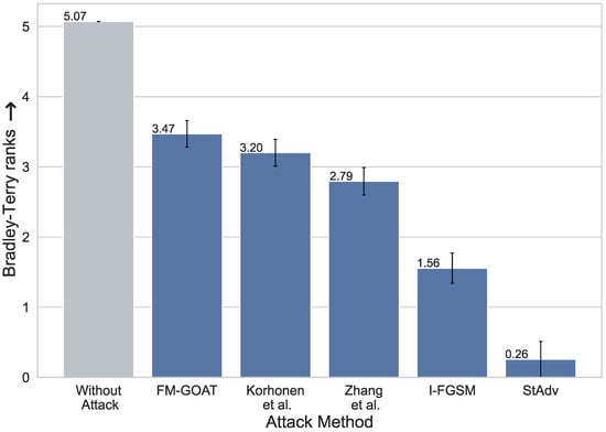
Figure 8.
Results of subjective pair-wise comparison of attack perceptibility. Values correspond to Bradley–Terry ranks (↑). For more details, please refer to Section 4.2.3.
4.3. Evaluating the Robustness of Different NR-IQA Models
To compare the robustness of IQA metrics to our proposed attack, we measured the maximum gain under fixed perturbation magnitude restrictions. For each test image, we used the highest value for the attack intensity parameter () that keeps the attacked image within selected constraints. We considered three constraint options: SSIM ≥ 0.99, LPIPS ≤ 0.01, and DISTS ≤ 0.01.
Evaluation methods. We quantify the robustness of the NR-IQA models via two key metrics: Absolute Gain, measuring the normalized increase in predicted quality scores, and the Robustness Score [55] (), which logarithmically scales the ratio of maximum permissible score deviation to the observed adversarial gain:
where and are the source and attacked images, and and are set to and 0, respectively.
The abs. gain measures the magnitude of the target model’s score inflation: high adversarial gain values correspond to drastic changes in model predictions after the attack, indicating significant vulnerability and lower model robustness. has an inverse meaning: higher values correspond to higher robustness. Although the attack’s goal is to inflate the target metric’s value on all images, we also report the Spearman correlation coefficient between metric values on source images and their adversarial counterparts to assess how well models preserve their original ranking under attack.
Table 3 presents results for different target NR-IQA models and different constraint types on the NIPS dataset. In this experimental setup, the PaQ-2-PiQ and MDTVSFA NR-IQA metrics emerge as the most resilient to the attack: they show the lowest adversarial gains (14.6% and 14.9% under the SSIM constraint) while maintaining moderate score consistency. TReS, Linearity, and CLIPIQA+, on the other hand, are the least stable, allowing for greater gains within the same loss level. Also noteworthy is that despite the strong adversarial gains, the TReS and TOPIQ models maintain a high correlation between their values before and after the attack, suggesting that even when the attack is a preprocessing routine for all input images, metrics can still differentiate low-quality images from high-quality ones. Although some models were more robust than others, none were able to completely withstand the attack without significant adversarial gains.
Table 3.
Robustness comparison of NR-IQA metrics under proposed attack, limited by the SSIM, LPIPS, and DISTS constraints on NIPS2017 dataset. Arrows describe the direction of better robustness, and the best results are highlighted in bold.
We also conduct an additional experiment with fixed attack strength on the KonIQ-10k IQA dataset [16]. Figure 9 shows the results, and more detailed evaluations can be found in Table A3a. As in the limited-visual-loss case, TReS, Linearity and CLIPIQA+ exhibit the highest adversarial gain (74.35%, 39.23% and 38.6%), while PaQ-2-PiQ and MDTVSFA show minimal score inflation (10.05% and 14.57%), but their predictions became inconsistent under the attack, demonstrating low correlation with their original image-quality estimates.
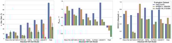
Figure 9.
Robustness comparison of NR-IQA models on Koniq-10k IQA and NIPS2017 image datasets and FullHD videos from Derf collection under fixed attack intensity. For videos, propagation method described in Section 3.3.2 is used. Evaluation metrics are described in Section 4.3.
To evaluate models on the video domain, we conduct a similar experiment on the Derf dataset [70] with a fixed parameter . We use the technique described in Section 3.3.2 to propagate our image-based attack through the videos while attacking only every 12th frame. For some models, the results differ among datasets, as Figure 9 and Table A3b show. Although MDTVSFA remains strongly robust and TReS remains highly vulnerable, Linearity and Hyper-IQA appear to be the most robust on high-resolution videos. This situation most likely owes to how these models handle high-resolution images. PaQ-2-PiQ processes images of any dimension as a set of independent “blocks” of predefined size, the number of which depends on the resolution, and the final score is an average of the block scores. TOPIQ in turn combines features of different scales. Apparently, such approaches lead to more efficient gradient propagation to the input image, which in turn leads to more efficient optimization during the attack. Linearity employs an adaptive pooling layer at the end of the convolutional network, allowing it to accept input images of any resolution, whereas Hyper-IQA scales all input images to 224 × 224. Therefore, both of these models clearly reduce the input data resolution by interpolating at some processing stage.
Figure 10 illustrates the trade-off between attack strength (), perceptual loss, and adversarial gain. For instance, TReS exhibits steeper gain increases than TOPIQ under similar SSIM degradation, underscoring its sensitivity to adversarial noise. These results collectively highlight that no model is fully robust, and architectural design—particularly resolution adaptation and feature aggregation—critically shapes resilience. Cross-dataset and cross-resolution evaluations remain essential, as robustness varies significantly with input characteristics.
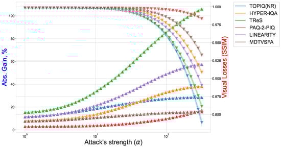
Figure 10.
Effect of step-size parameter on attack efficiency (Absolute Gain) and visual losses (SSIM). Solid line with △ symbols indicates efficiency changes; dashed line with ▽ symbols indicates losses.
4.4. Transferability of Adversarial Examples
To test the transferability of the adversarial examples between the NR-IQA models, we chose one model as a proxy optimization target of the attack and measured the Absolute Gain for the others. In this experiment, we fixed the attack strength parameter, , at 50 for all images and proxy models. Figure 11 presents the results of this evaluation.
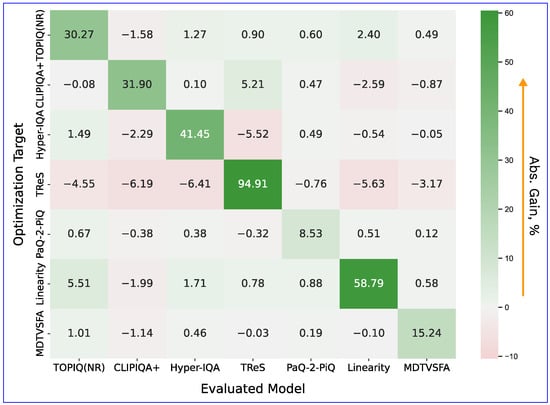
Figure 11.
Transferability of adversarial examples between NR-IQA models, measured with Absolute Gain. Rows denote models that serve as a proxy during the attack, and columns correspond to different evaluated models. Higher values indicate stronger attack effect.
We found that adversarial examples exhibit weak transferability between IQA models. This finding correlates with the results of [55]: the authors discovered poor adversarial example transferability for a different attack and set of NR-IQA models. Apparently, pixel space white box attacks exploit specific architectural vulnerabilities unique to each NR-IQA model. Also noteworthy is that metrics using the same backbone CNN architecture fail to show increased transferability among themselves. This result is potentially because the adversarial additive implicitly seeks to distort the outputs of the final network layers (which vary from model to model), and therefore corresponding distortions of the backbone network outputs lose adversarial efficiency. Section 4.6 further investigates this hypothesis.
4.5. Defending NR-IQA Models with Input Transformations
This section evaluates the efficiency of common adversarial purification techniques applied to NR-IQA metrics. These techniques employ input transformations as a preprocessing step to “erase” potential adversarial additives from the image. Evaluated methods include bilinear upscale, image enhancement using RealESRGAN [78], flip (image reflection along the y-axis), Gaussian blur (with 3 × 3 kernel and ), random rotation (up to 15 degrees), random crop (256 × 256), JPEG-compression defense (with quality factors q = 50 and q = 75), median filtering (3 × kernel), and feature squeezing [79] (color quantization to 4 bits per channel).
To evaluate adversarial defenses, we measure Absolute Gain and , defined in (16), after applying transformations to both the attacked image and the original image. We also report the Spearman correlation coefficient between metric values for the original images, before and after applying the defense, to evaluate the quality score distortion caused by this preprocessing step. We use two highly vulnerable models from prior analyses, Linearity and TReS, as attack targets in this experiment. The results are presented in Figure 12 and described in more detail in Table A4.
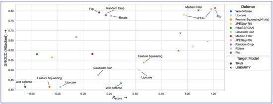
Figure 12.
Performance of different defensive image transformations on Linearity and TReS metrics in nonadaptive scenario (i.e., the attacker is unaware of the defense method). Colors represent different defensive methods, and × and · dot types correspond to LINEARITY and TReS target models used during the attack.
Simple “spatial” transformations, such as flip and rotate, are among the most efficient at reducing metric gains on adversarial examples—a common feature of adversarial perturbations obtained using white box optimization in pixel space. Compression and filtering can also limit the attack’s efficacy, but no method in our investigation completely erased the adversarial effect. Furthermore, most effective defenses alter the metric scores on the original images—as measured by SROCC (clear)—as they significantly alter the perceived image quality, therefore making them impractical for IQAs.
Defenses assume attackers lack knowledge of preprocessing steps. When aware, adversaries can adapt by incorporating transformations into the attack loop. To demonstrate this vulnerability, we attempted to bypass the adversarial defenses for flip, Gaussian blur, random rotation, and JPEG compression by modifying the loss function L used to compute the target model’s gradient during attack. We used an average metric value for the original and corresponding defended image as our optimization target. Flip, blur, and rotate are differentiable operations, and for compression, we used DiffJPEG [80] (a differentiable approximation of the JPEG algorithm) with a matching quality factor. These simple modifications of the attack can, in some cases, greatly diminish the effectiveness of corresponding defenses (see Table 4). For simple differentiable operations (flip, blur, and rotation), modifying the loss to target both for original and transformed images can reduce defense efficacy by up to 90%. Noticeably, differentiable JPEG approximation shows limited bypass success on JPEG compression, diverging from the results for classifiers [80].
Table 4.
Efficiency of different defenses in adaptive scenario: adversarial attack was adopted to bypass corresponding purification methods. TOPIQ NR-IQA model is used as a target. Each transformation denoted in the top row was incorporated into the attack to reduce the efficiency of the corresponding purification method.
4.6. Analyzing Attack Effectiveness
This section presents observations as well as hypotheses we empirically tested as we studied IQA metric robustness. Our analysis focuses on features that correlate highly with the adversarial efficiency of the attacks, which may be useful for detecting NR-IQA model failure modes and countering adversarial threats.
4.6.1. Attack Susceptibility and Initial Scores
Figure 13a demonstrates that images with lower initial quality scores (as predicted by the target model) are more vulnerable to score inflation, although most of the considered metrics do not strictly limit the output value range. Notably, TReS and Linearity implement novel loss designs (self-consistency and relative ranking in the former, norm-in-norm in the latter) alongside classic regression MAE/MSE loss functions, which may partially explain why they are easier to manipulate beyond their normal ranges and the correlation with initial metric values is less prominent.
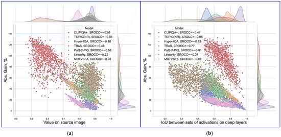
Figure 13.
Correlations between Absolute Gain (attack efficiency) and (a) target model value for original image and (b) IoU measured between sets of neuron activations for original and attacked images on specific model layers. Each point represents a single attacked image. Source images are from NIPS2017 dataset.
4.6.2. Perturbation Propagation in Feature Space
We found empirically that adversarial perturbations induce cumulative distortions in target model activations, diverging progressively across network layers. Figure 14a quantifies this effect using style loss [81], a popular measure for stylistic proximity between images, which evaluates the discrepancy between Gram matrices of clean and attacked activations:
where represents activations of model f from layer m (with c channels and features within each of them), and represents activations from the model’s ith channel. and are activations collected from source and attacked images, respectively.
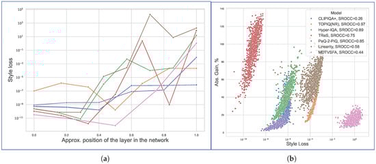
Figure 14.
(a) Mean style loss between model activations for original and attacked images measured at different neural network layers. Lines represent different NR-IQA models. Layer depth increases from left to right; greater style loss corresponds to greater divergence in layer outputs. (b) Correlation between attack efficiency (Absolute Gain) and style loss on penultimate layer of NR-IQA models.
For each metric, we selected a set of approximately equidistant layers located throughout the model. Since each model has a unique architecture, accurately collating layers for different IQA metrics is non-trivial, and therefore the x-coordinate in the figure only quantifies the layer’s relative network position. However, the distance between activations generally demonstrates an increasing trend, indicating that adversarial perturbations disproportionately alter high-level semantic features. Moreover, the activations for attacked examples in the last few layers can be easily distinguished from clear instances without calculating the final network output (see Figure 15). This observation may facilitate the identification of adversarial attacks using anomaly detection methods [82].
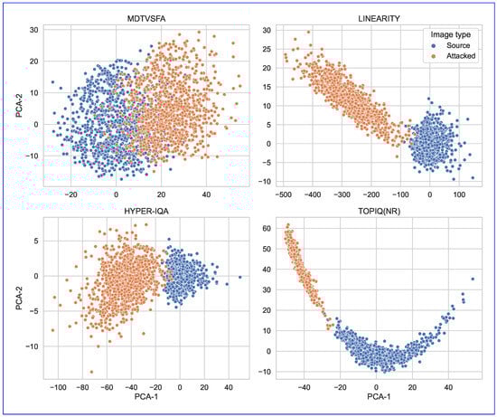
Figure 15.
Two-component PCA of NR-IQA model activations from penultimate layers for the original and corresponding adversarial images. PCA is fitted only on source activations. For most models, the activations for adversarial examples are reliably differentiable from those for the original images.
The PCA of penultimate-layer activations (Figure 15) confirms that adversarial examples occupy distinct regions in feature space, separable from clean images despite minimal pixel-level differences. This divergence underscores the vulnerability of deep representations to malicious perturbations.
4.6.3. Activation Patterns and Attack Efficacy
We empirically found that the attack’s success correlates more strongly with which neurons activate rather than with their exact output values. To assess this factor, we examine the difference in sets of activated neurons when calculating the final metric value for the original and attacked images. Since we selected the layers to include an activation function at the end (where applicable), we consider a neuron with a positive output to be activated. To measure the activation differences, we applied the intersection over union (IoU) over the sets of activated neurons for a given image before and after the attack.
As Figure 13b shows, higher IoU reduction corresponds to greater adversarial gains. Note that this value is quantized and does not capture the neurons’ output values; it only captures binarized activations, and at the same time, it clearly correlates with the attack’s effectiveness. This observation suggests that attacks might exploit specific activation pathways rather than gradual neuron output shifts.
5. Ablation Study
5.1. Effects of Gradient Correction
Impact of Constraint Combinations. To quantify the impact of gradient correction and constraint selection, we compare our method against an unconstrained baseline and variants using individual or combined constraints . All experiments fix and 15 iterations on the Linearity target model. Table 5 presents the results.
Table 5.
Ablation study on effects of high-frequency masking and incorporation of different constraint function combinations (identified in leftmost column) into attack’s gradient-correction step. Percentage values represent change in corresponding measurements relative to “Baseline (w/o constraints)” case.
Adding the SSIM alone reduces perceptual losses by 20–25%, as measured by more complex FR models (LPIPS, DISTS, and PieAPP), but decreases adversarial gain by 12%, as strict structural preservation limits the perturbation magnitude. LPIPS proves most effective for its intended metric, halving LPIPS perceptual loss (−52%) with minimal gain reduction (−1.14%), while also improving DISTS and PieAPP losses (−6-7%). The optimal trade-off emerges with LPIPS + SSIM + , achieving near-maximal loss reduction (LPIPS: −53.79%, DISTS: −30.05%, and PieAPP: −29.62%). This combination leverages the SSIM and for low-level structural fidelity and LPIPS for high-level perceptual alignment, with minimal computational overhead compared to more complex learning-based constraints like DISTS or PieAPP. Combined with the SSIM and , LPIPS shows the best transferability of the regularization effect to other deep FR metrics.
Gradient Direction and Magnitude. To evaluate the effect of gradient correction on the attack direction in pixel space, we measure average cosine similarities between target model gradients before and after applying the correction, as well as constraint functions during the attack. As the adversarial additive is initialized with zeros and, therefore, the constraint gradients are zero vectors at the start of the optimization, we omit the first iteration when averaging.
Figure 16a reveals high similarity (0.85–0.92) between corrected and uncorrected gradients, confirming that orthogonalization preserves the attack’s primary direction while mitigating collateral perceptual damage. Constraint gradients exhibit low mutual similarity (0.1–0.3), indicating they capture distinct distortion aspects. Post-correction gradients retain 70–90% of their original magnitude (Figure 16b), ensuring efficient optimization despite constraint enforcement.
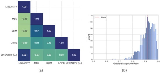
Figure 16.
(a) Mean cosine similarity between gradients of different models used in attack. Linearity model is a target in this experiment. Linearity (⊥) denotes target model’s gradient after the proposed correction step. (b) Ratio of target IQA model’s (Linearity) gradient magnitudes before and after gradient correction on NIPS2017 dataset. Values close to 1 indicate the gradient magnitude was mitigated insignificantly during the correction and therefore can still be used to optimize the image.
5.2. Comparing Video Propagation Methods
We compare the visual losses and adversarial gain for FM-GOAT combined with different propagation methods: attack on each individual frame (or every nth frame), interpolation of the adversarial perturbation between evenly spaced attacked frames, and repetition from the last attacked frame. Interpolation and repetition approaches are compared with and without the motion compensation. For each approach (except the attack on all frames), we applied an image-based attack to every 12th frame and propagated it to intermediate frames using the corresponding method.
Table 6 presents the comparison results. The approach described in Section 3.3.2 (highlighted in bold) maintains a reasonable balance between computational complexity, objective visual losses, temporal smoothness of the adversarial additive, and the adversarial gain. The attack on all frames individually scales the adversarial gain (and computational cost) almost proportionally, but it also introduces visible temporal flickering artifacts. Interpolation without motion compensation generates temporally smooth additives but creates visible distortions when motion causes the adversarial additive to extend beyond the information-rich regions. Repetition of the adversarial perturbation from the previous attacked keyframe introduces noticeable sudden changes and is less efficient than interpolation in terms of adversarial gain.
Table 6.
Comparison of different video propagation methods on Derf dataset and MDTVSFA target IQA model. “Interpolation + Motion Comp.” denotes our proposed propagation method.
6. Discussion
6.1. Robustness of NR-IQA Models
Our evaluations show that all tested NR-IQA models can be manipulated with the proposed attack to inflate their scores. While attention-based metrics (TOPIQ, TReS, and CLIPIQA+) demonstrated lower robustness to the proposed attack, we suggest it might be partially related to specific architectural designs of these models, e.g., the multiscale approach in TOPIQ and self-consistency training in TReS. The Vision–Language perspective implemented in CLIPIQA+ also does not prevent the model from being manipulated. The most robust IQA models in our tests (PaQ-2-PiQ and MDTVSFA) utilize a relatively simple CNN-based architecture with ResNet backbones for feature extraction. We hypothesize that smaller models with lower parameter counts and localized feature extraction might be generally more resilient to adversarial examples, likely due to a lower amount of available input–output pathways within a model that could be exploited by the attack; however, a more detailed further inquiry is required to test this assumption in more general scenarios.
We empirically discovered that for some models, robustness also varies with input resolution, likely due to specific methods for variable resolution input handling. For instance, the Linearity model uses adaptive pooling for internal activations, and its robustness increases with higher resolution. Aside from model-specific properties and design choices, we focused on more general model behavior trends in adversarial scenarios and discovered several patterns that are common to all tested models despite their architectural differences.
6.2. Cross-Model Patterns
We empirically found out that adversarial attacks universally have a cumulative effect on IQA models’ layer outputs—a non-trivial observation that might encourage IQA researchers to pay more attention to the stability of internal layer activations in the new models and propose defensive strategies that will detect adversarial activations and purify them. We further demonstrate that IQA models’ internal representations of adversarial examples diverge significantly from those of ordinary images (Figure 15), and this behavior is present among models of different architectures. This indicates that adversarial attacks push model activations outside of their regular distributions, and anomaly detection methods can potentially be used in the model’s activation space to detect malicious input manipulations. It might be an important research direction for NR-IQA adversarial robustness, and we leave it for future studies.
Additionally, we analyzed the correlations between the adversarial efficiency of the attack and different statistics collected from models’ layer activations. Interestingly, our findings reveal that adversarial gain strongly correlates with the share of neurons that were “flipped” from inactive to active and vice versa, rather than their specific values. Novel adversarial training techniques can be proposed to utilize this property and penalize instability in the model’s activations.
6.3. Defenses Evaluation
We have also tested multiple common input preprocessing techniques to assess their efficiency in mitigating adversarial perturbations. Our experiments suggest that input preprocessing transformations can substantially improve the robustness of IQA models; however, they can noticeably degrade image quality, and therefore distort quality scores on non-attacked images. Furthermore, most of the defenses can be successfully bypassed if the attacker has knowledge of the defensive technique employed in the model. We also note that the topic of adversarial defenses for IQAs has recently been explored in more detail by Gushchin et al. [83], and our results align well with their findings.
7. Conclusions
This work introduces FM-GOAT, an iterative white box adversarial attack tailored for no-reference Image Quality Assessment (NR-IQA) models. By integrating multiple differentiable constraints, we bypass traditional -norm limitations, enforcing imperceptibility through perceptual alignment rather than rigid magnitude thresholds. The proposed gradient orthogonalization technique eliminates hyperparameter tuning and reduces the attack’s collateral effect on constraining functions without directly optimizing them, while high-frequency masking and motion-aware video propagation minimize visible artifacts across spatial and temporal domains. Our approach allows the attack to generate norm-unconstrained adversarial examples that exploit the target IQA metric’s vulnerabilities while minimizing perceptual losses.
Our extensive experiments on six NR-IQA models of different architectures demonstrate the effectiveness of the proposed attack. We show that all these metrics are subject to manipulation, and their quality predictions can be severely inflated even under a strictly constrained perturbation budget. However, adversarial examples exhibit weak transferability between architectures, indicating that vulnerabilities are model-specific and tied to unique feature-processing pathways. Furthermore, we evaluate the NR-IQA metrics’ robustness when employing common adversarial purification defensive techniques, such as image transformations and filtering.
Overall, we highlight the importance of developing robust and reliable IQA models that can withstand adversarial threats—whether through architectural hardening, input preprocessing, or anomaly detection in feature space. The proposed method, along with the insights highlighted in our NR-IQA failure mode analysis, can inform future research toward building more secure and more trustworthy visual quality evaluation systems.
8. Future Work
8.1. Multitask Adversarial Scenarios
Our proposed gradient-projection method allows an attack to serve in a multitask scenario—for example, if the goal is to deceive an IQA (or any other) model while preserving the performance of classification, object detection, or other models. Examining the collateral effects of adversarial attacks on models designed for other tasks (especially if they have a similar backbone network) may be an important area for further research.
8.2. Interpretable Feature Defense
Furthermore, we still lack understanding of the features from deep layers of learning-based IQA models and are therefore unable to properly interpret the effects of adversarial attacks on their behavior. Researchers have made recent progress in obtaining interpretable (monosemantic) features from Transformer-based multimodal Large Language Models [84] via sparse autoencoders (SAEs); this method is potentially applicable to IQA metrics as well as other computer vision tasks [85,86]. Exploring the impact of adversarial attacks on a meaningful set of "concepts" that the model considers when making a prediction could be helpful for further advancement toward more robust models.
Author Contributions
K.A.: conceptualization, data curation, formal analysis, investigation, software, visualization, and writing—original draft. S.L.: methodology, project administration, supervision, validation, and writing—review and editing. D.V.: funding acquisition and supervision. All authors have read and agreed to the published version of the manuscript.
Funding
This work was supported by the Ministry of Economic Development of the Russian Federation (code 25-139-66879-1-0003).
Data Availability Statement
The data presented in this study are openly available at https://github.com/X1716/FM-GOAT. All evaluations in this work were conducted using publicly available datasets. They can be accessed through the corresponding project pages: NIPS2017 [69], KonIQ-10k [16], and Derf [70].
Acknowledgments
The evaluations for this research were carried out using the MSU-270 supercomputer of Lomonosov Moscow State University.
Conflicts of Interest
The authors declare no conflicts of interest.
Appendix A. Attack Algorithm
Algorithm A1 describes in pseudocode the overall procedure of our adversarial attack, and Algorithm A2 describes the function for obtaining the high-frequency mask.
| Algorithm 1: FM-GOAT |
|
|
| Algorithm 2: |
|
Appendix B. Time Complexity Comparison
Table A1 contains compute time evaluations for the adversarial attacks in our comparison. Each value is the mean of seven sets of 10 launches. We took all measurements using the same setup that includes an Nvidia GeForce RTX 4080 GPU and an Intel Core i7 8700 processor. The I-FGSM attack is the fastest, as it lacks any complicated operations besides single backpropagation steps through the target model per iteration. Our attack achieves a speed similar to that of competitors but is a bit slower, owing to the gradient correction and corresponding calculation of the LPIPS, SSIM, and gradients.
These measurements also show that the models vary in gradient computation speed: PaQ-2-PiQ is the fastest, whereas the attacks on the Linearity and TOPIQ metrics take up to 3–4 times longer.
Table A2 presents peak VRAM usage during the attacks for different target models. All attacks have fairly similar memory usage when attacking the same IQA model, as it mostly depends on the model size. However, it could be seen that the Zhang et al. attack consistently consumes slightly more memory, as it uses the DISTS FR-IQA model for regularization.
Table A1.
Computational speed of different white box adversarial attacks for different target IQA models.
Table A1.
Computational speed of different white box adversarial attacks for different target IQA models.
| Model | # of Iters | Attack | ||||
|---|---|---|---|---|---|---|
| FM-GOAT | Korhonen et al. | I-FGSM | Zhang et al. | StAdv | ||
| Hyper-IQA | 3 | 172 ± 6.17 ms | 105 ± 1.22 ms | 102 ± 1.76 ms | 156 ± 5.23 ms | 147 ± 5.19 ms |
| 10 | 486 ± 15.2 ms | 320 ± 3.57 ms | 321 ± 5.04 ms | 498 ± 7.13 ms | 480 ± 8.76 ms | |
| Linearity | 3 | 280 ± 7.23 ms | 214 ± 4.99 ms | 207 ± 3.01 ms | 261 ± 4.6 ms | 271 ± 8.67 ms |
| 10 | 851 ± 9.3 ms | 710 ± 16 ms | 690 ± 6.94 ms | 873 ± 18.1 ms | 885 ± 21.2 ms | |
| MDTVSFA | 3 | 156 ± 3.29 ms | 98.2 ± 2.58 ms | 92.2 ± 2.22 ms | 146 ± 3.42 ms | 13 ± 7.65 ms |
| 10 | 466 ± 5.03 ms | 295 ± 3.77 ms | 292 ± 4.71 ms | 469 ± 17.2 ms | 466 ± 9.96 ms | |
| PAQ-2-PIQ | 3 | 99.6 ± 5.28 ms | 47 ± 2 ms | 38.9 ± 0.7 ms | 95.4 ± 2.94 ms | 86.5 ± 4.8 ms |
| 10 | 294 ± 7.32 ms | 136 ± 2.8 ms | 127 ± 2.17 ms | 320 ± 15.8 ms | 271 ± 18 ms | |
| TOPIQ(NR) | 3 | 273 ± 7.24 ms | 204 ± 3.13 ms | 198 ± 5.68 ms | 253 ± 4.78 ms | 258 ± 12.9 ms |
| 10 | 777 ± 6.31 ms | 640 ± 19 ms | 608 ± 4.74 ms | 780 ± 7.51 ms | 795 ± 12.1 ms | |
| TReS | 3 | 236 ± 6.22 ms | 194 ± 3.75 ms | 188 ± 2.9 ms | 254 ± 5.17 ms | 210 ± 5.86 ms |
| 10 | 754 ± 11.7 ms | 591 ± 10.9 ms | 585 ± 13.1 ms | 857 ± 17.6 ms | 693 ± 23.8 ms | |
Table A2.
Peak GPU memory usage (in MB, ↓) during the attack, evaluated for different target IQA models and adversarial attacks.
Table A2.
Peak GPU memory usage (in MB, ↓) during the attack, evaluated for different target IQA models and adversarial attacks.
| Model | I-FGSM | StAdv | Korhonen et al. | Zhang et al. | FM-GOAT |
|---|---|---|---|---|---|
| Hyper-IQA | 2469.54 | 2467.65 | 2409.25 | 2689.00 | 2485.45 |
| Linearity | 1403.05 | 1403.05 | 1403.05 | 1533.07 | 1412.10 |
| MDTVSFA | 384.79 | 382.41 | 393.92 | 721.90 | 400.04 |
| PAQ-2-PIQ | 169.96 | 169.95 | 194.65 | 522.90 | 187.95 |
| TOPIQ(NR) | 646.94 | 641.76 | 665.90 | 994.72 | 668.73 |
| TReS | 1632.11 | 1628.14 | 1435.09 | 1687.89 | 1651.59 |
Appendix C. Additional Results
Table A3 presents the results of a robustness comparison of the NR-IQA models on the KonIQ-10k and Derf datasets, discussed in Section 4.2.2.
Table A4 demonstrates the detailed results of different defensive input transformations for adversarial attack mitigation in a nonadaptive scenario.
Table A3.
Robustness comparison of NR-IQA models on (a) Koniq-10k IQA dataset and (b) FullHD videos from Derf dataset under fixed attack intensity. For videos, propagation method described in Section 3.3.2 is used. The best results are highlighted in bold.
Table A3.
Robustness comparison of NR-IQA models on (a) Koniq-10k IQA dataset and (b) FullHD videos from Derf dataset under fixed attack intensity. For videos, propagation method described in Section 3.3.2 is used. The best results are highlighted in bold.
| (a) | ||||
|---|---|---|---|---|
| Score | Abs. Gain↓ | Rscore↑ | SROCC↑ (Attacked) | |
| Target Model | ||||
| TOPIQ(NR) | 32.87 ± 12.98% | 0.325 | 0.538 | |
| Hyper-IQA | 28.28 ± 10.98% | 0.390 | 0.551 | |
| TReS | 74.35 ± 19.88% | −0.701 | 0.395 | |
| PAQ-2-PIQ | 10.05 ± 5.76% | 0.921 | 0.395 | |
| Linearity | 39.32 ± 14.15% | 0.226 | 0.425 | |
| MDTVSFA | 14.57 ± 4.18% | 0.606 | 0.162 | |
| CLIPIQA+ | 38.60 ± 13.9 | 0.248 | 0.462 | |
| (b) | ||||
| Score | Abs. Gain↓ | Rscore↑ | SROCC↑ (Attacked) | |
| Target Model | ||||
| TOPIQ(NR) | 13.60 ± 5.95% | 0.734 | 0.845 | |
| Hyper-IQA | 6.17 ± 3.61% | 1.093 | 0.700 | |
| TReS | 24.35 ± 18.75% | −0.127 | 0.405 | |
| PAQ-2-PIQ | 13.41 ± 7.65% | 0.742 | 0.676 | |
| Linearity | 2.80 ± 3.37% | 1.415 | 0.983 | |
| MDTVSFA | 5.89 ± 3.13% | 1.029 | 0.644 | |
| CLIPIQA+ | 13.74 ± 7.6% | 0.762 | 0.778 | |
Table A4.
Performance of different defensive image transformations on Linearity and TReS metrics in nonadaptive scenario (i.e., the attacker is unaware of the defense method). The best results are highlighted in bold.
Table A4.
Performance of different defensive image transformations on Linearity and TReS metrics in nonadaptive scenario (i.e., the attacker is unaware of the defense method). The best results are highlighted in bold.
| Target Model Score | Linearity | TReS | |||||||
|---|---|---|---|---|---|---|---|---|---|
| Defense | Abs. Gain↓ | Rscore↑ | SROCC↑ (Clear) | SROCC↑ (Attacked) | Abs. Gain↓ | Rscore↑ | SROCC↑ (Clear) | SROCC↑ (Attacked) | |
| W/o defense | 33.09 ± 0.33% | 0.363 | - | 0.432 | 56.80 ± 0.67% | −0.557 | - | 0.414 | |
| Upscale | 21.06 ± 0.28% | 0.541 | 0.941 | 0.500 | 44.54 ± 0.59% | −0.219 | 0.983 | 0.414 | |
| Feature squeezing (4 bits) | 18.78 ± 0.25% | 0.582 | 0.900 | 0.537 | 43.85 ± 0.63% | −0.324 | 0.974 | 0.414 | |
| RealESRGAN | 10.63 ± 0.19% | 0.916 | 0.886 | 0.597 | 30.92 ± 0.57% | −0.444 | 0.963 | 0.580 | |
| Random crop | 10.58 ± 0.23% | 0.934 | 0.968 | 0.687 | 13.92 ± 0.30% | 0.217 | 0.962 | 0.778 | |
| JPEG (q = 75) | 7.88 ± 0.13% | 0.967 | 0.921 | 0.781 | 33.34 ± 0.52% | −0.299 | 0.971 | 0.563 | |
| Rotate | 6.37 ± 0.24% | 1.194 | 0.877 | 0.644 | 12.90 ± 0.38% | 0.269 | 0.913 | 0.775 | |
| Median filter | 5.89 ± 0.10% | 1.107 | 0.875 | 0.803 | 25.03 ± 0.40% | 0.089 | 0.917 | 0.581 | |
| Gaussian blur | 5.55 ± 0.10% | 1.055 | 0.752 | 0.619 | 28.37 ± 0.44% | 0.145 | 0.929 | 0.474 | |
| Flip | 4.60 ± 0.10% | 1.266 | 0.886 | 0.814 | 12.41 ± 0.23% | 0.154 | 0.947 | 0.792 | |
| JPEG(q = 50) | 4.09 ± 0.08% | 1.230 | 0.849 | 0.809 | 23.89 ± 0.38% | -0.067 | 0.949 | 0.667 | |
References
- Wang, Z.; Bovik, A.; Sheikh, H.; Simoncelli, E. Image quality assessment: From error visibility to structural similarity. IEEE Trans. Image Process. 2004, 13, 600–612. [Google Scholar] [CrossRef] [PubMed]
- Zhang, R.; Isola, P.; Efros, A.A.; Shechtman, E.; Wang, O. The Unreasonable Effectiveness of Deep Features as a Perceptual Metric. In Proceedings of the CVPR, Salt Lake City, UT, USA, 19-21 June 2018. [Google Scholar]
- Ding, K.; Ma, K.; Wang, S.; Simoncelli, E.P. Image Quality Assessment: Unifying Structure and Texture Similarity. IEEE Trans. Pattern Anal. Mach. Intell. 2022, 44, 2567–2581. [Google Scholar] [CrossRef]
- Startsev, V.; Ustyuzhanin, A.; Kirillov, A.; Baranchuk, D.; Kastryulin, S. Alchemist: Turning Public Text-to-Image Data into Generative Gold. arXiv 2025, arXiv:2505.19297. Available online: http://arxiv.org/abs/2505.19297 (accessed on 8 June 2025).
- V-Nova. FFmpeg with LCEVC. 2023. Available online: https://v-nova.com/press-releases/globo-deploys-lcevc-enhanced-stream-for-2023-brazilian-carnival/ (accessed on 1 May 2025).
- Phadikar, B.; Phadikar, A.; Thakur, S. A comprehensive assessment of content-based image retrieval using selected full reference image quality assessment algorithms. Multimed. Tools Appl. 2021, 80, 15619–15646. [Google Scholar] [CrossRef]
- Yang, Y.; Jiao, S.; He, J.; Xia, B.; Li, J.; Xiao, R. Image retrieval via learning content-based deep quality model towards big data. Future Gener. Comput. Syst. 2020, 112, 243–249. [Google Scholar] [CrossRef]
- Abud, K.; Lavrushkin, S.; Kirillov, A.; Vatolin, D. IQA-Adapter: Exploring Knowledge Transfer from Image Quality Assessment to Diffusion-based Generative Models. arXiv 2024, arXiv:2412.01794. Available online: http://arxiv.org/abs/2412.01794 (accessed on 8 June 2025).
- Zhu, H.; Li, L.; Wu, J.; Dong, W.; Shi, G. MetaIQA: Deep Meta-Learning for No-Reference Image Quality Assessment. In Proceedings of the IEEE Conference on Computer Vision and Pattern Recognition (CVPR), Virtual Conference, 16–18 June 2020; pp. 14143–14152. [Google Scholar]
- Goodfellow, I.J.; Shlens, J.; Szegedy, C. Explaining and harnessing adversarial examples. arXiv 2014, arXiv:1412.6572. [Google Scholar]
- Ma, W.; Li, Y.; Jia, X.; Xu, W. Transferable Adversarial Attack for Both Vision Transformers and Convolutional Networks via Momentum Integrated Gradients. In Proceedings of the 2023 IEEE/CVF International Conference on Computer Vision (ICCV), Paris, France, 2–3 October 2023; pp. 4607–4616. [Google Scholar] [CrossRef]
- Bai, T.; Luo, J.; Zhao, J.; Wen, B.; Wang, Q. Recent Advances in Adversarial Training for Adversarial Robustness. In Proceedings of the Thirtieth International Joint Conference on Artificial Intelligence (IJCAI-21), Virtual Conference, 19–26 August 2021; pp. 4312–4321. [Google Scholar] [CrossRef]
- Papernot, N.; McDaniel, P.; Wu, X.; Jha, S.; Swami, A. Distillation as a Defense to Adversarial Perturbations Against Deep Neural Networks. In Proceedings of the Proceedings—2016 IEEE Symposium on Security and Privacy (SP 2016), San Jose, CA, USA, 23–25 May 2016; pp. 582–597. [Google Scholar] [CrossRef]
- Nie, W.; Guo, B.; Huang, Y.; Xiao, C.; Vahdat, A.; Anandkumar, A. Diffusion Models for Adversarial Purification. In Proceedings of the International Conference on Machine Learning (ICML), Honolulu, HI, USA, 23–29 July 2022. [Google Scholar]
- Li, D.; Jiang, T.; Jiang, M. Norm-in-norm loss with faster convergence and better performance for image quality assessment. In Proceedings of the 28th ACM International Conference on Multimedia, Seattle, WA, USA, 12–16 October 2020; pp. 789–797. [Google Scholar]
- Hosu, V.; Lin, H.; Szirányi, T.; Saupe, D. KonIQ-10k: An Ecologically Valid Database for Deep Learning of Blind Image Quality Assessment. IEEE Trans. Image Process. 2020, 29, 4041–4056. [Google Scholar] [CrossRef]
- Li, Z.; Aaron, A.; Katsavounidis, I.; Manohara, M. Toward A Practical Perceptual Video Quality Metric. 2016. Available online: https://netflixtechblog.com/toward-a-practical-perceptual-video-quality-metric-653f208b9652 (accessed on 1 May 2024).
- Kashkarov, E.; Chistov, E.; Molodetskikh, I.; Vatolin, D. Can No-Reference Quality-Assessment Methods Serve as Perceptual Losses for Super-Resolution? arXiv 2024, arXiv:eess.IV/2405.20392. Available online: http://arxiv.org/abs/2405.20392 (accessed on 23 April 2025).
- Chen, J.; Chen, H.; Chen, K.; Zhang, Y.; Zou, Z.; Shi, Z. Diffusion Models for Imperceptible and Transferable Adversarial Attack. IEEE Trans. Pattern Anal. Mach. Intell. 2025, 47, 961–977. [Google Scholar] [CrossRef]
- Dai, X.; Liang, K.; Xiao, B. AdvDiff: Generating Unrestricted Adversarial Examples using Diffusion Models. arXiv 2023, arXiv:2307.12499. [Google Scholar]
- Yang, X.; Li, F.; Zhang, W.; He, L. Blind Image Quality Assessment of Natural Scenes Based on Entropy Differences in the DCT Domain. Entropy 2018, 20, 885. [Google Scholar] [CrossRef] [PubMed]
- Oszust, M.; Piórkowski, A.; Obuchowicz, R. No-reference image quality assessment of magnetic resonance images with high-boost filtering and local features. Magn. Reson. Med. 2020, 84, 1648–1660. [Google Scholar] [CrossRef] [PubMed]
- Mittal, A.; Moorthy, A.K.; Bovik, A.C. No-Reference Image Quality Assessment in the Spatial Domain. IEEE Trans. Image Process. 2012, 21, 4695–4708. [Google Scholar] [CrossRef]
- Kang, L.; Ye, P.; Li, Y.; Doermann, D. Convolutional Neural Networks for No-Reference Image Quality Assessment. In Proceedings of the 2014 IEEE Conference on Computer Vision and Pattern Recognition (CVPR ’14), Columbus, OH, USA, 24–27 June 2014; pp. 1733–1740. [Google Scholar] [CrossRef]
- He, K.; Zhang, X.; Ren, S.; Sun, J. Deep Residual Learning for Image Recognition. In Proceedings of the 2016 IEEE Conference on Computer Vision and Pattern Recognition (CVPR), Las Vegas, NV, USA, 26 June–1 July 2016; pp. 770–778. [Google Scholar] [CrossRef]
- Tan, M.; Le, Q.V. EfficientNet: Rethinking Model Scaling for Convolutional Neural Networks. arXiv 2020, arXiv:cs.LG/1905.11946. Available online: http://arxiv.org/abs/1905.11946 (accessed on 25 April 2025).
- Ying, Z.a.; Niu, H.; Gupta, P.; Mahajan, D.; Ghadiyaram, D.; Bovik, A. From Patches to Pictures (PaQ-2-PiQ): Mapping the Perceptual Space of Picture Quality. arXiv 2019, arXiv:1912.10088. [Google Scholar]
- Su, S.; Yan, Q.; Zhu, Y.; Zhang, C.; Ge, X.; Sun, J.; Zhang, Y. Blindly assess image quality in the wild guided by a self-adaptive hyper network. In Proceedings of the IEEE/CVF Conference on Computer Vision and Pattern Recognition, Virtual Conference, 16–18 June 2020; pp. 3667–3676. [Google Scholar]
- Li, D.; Jiang, T.; Jiang, M. Quality Assessment of In-the-Wild Videos. In Proceedings of the 27th ACM International Conference on Multimedia, Nice, France, 21–25 October 2019; pp. 2351–2359. [Google Scholar] [CrossRef]
- Li, D.; Jiang, T.; Jiang, M. Unified quality assessment of in-the-wild videos with mixed datasets training. Int. J. Comput. Vis. 2021, 129, 1238–1257. [Google Scholar] [CrossRef]
- Wu, H.; Chen, C.; Liao, L.; Hou, J.; Sun, W.; Yan, Q.; Gu, J.; Lin, W. Neighbourhood Representative Sampling for Efficient End-to-end Video Quality Assessment. arXiv 2022, arXiv:2210.05357. Available online: http://arxiv.org/abs/2210.05357 (accessed on 5 April 2025). [CrossRef]
- Wu, H.; Chen, C.; Hou, J.; Liao, L.; Wang, A.; Sun, W.; Yan, Q.; Lin, W. FAST-VQA: Efficient End-to-end Video Quality Assessment with Fragment Sampling. In Proceedings of the European Conference of Computer Vision (ECCV), Tel Aviv, Israel, 23–27 October 2022. [Google Scholar]
- Chen, C.; Mo, J.; Hou, J.; Wu, H.; Liao, L.; Sun, W.; Yan, Q.; Lin, W. TOPIQ: A Top-down Approach from Semantics to Distortions for Image Quality Assessment. arXiv 2023, arXiv:2308.03060. [Google Scholar] [CrossRef]
- Golestaneh, S.A.; Dadsetan, S.; Kitani, K.M. No-reference image quality assessment via transformers, relative ranking, and self-consistency. In Proceedings of the IEEE/CVF Winter Conference on Applications of Computer Vision, Waikoloa, HI, USA, 4–8 January 2022; pp. 1220–1230. [Google Scholar]
- Wu, H.; Zhang, Z.; Zhang, W.; Chen, C.; Li, C.; Liao, L.; Wang, A.; Zhang, E.; Sun, W.; Yan, Q.; et al. Q-Align: Teaching LMMs for Visual Scoring via Discrete Text-Defined Levels. arXiv 2023, arXiv:2312.17090. [Google Scholar]
- Miyata, T. ZEN-IQA: Zero-Shot Explainable and No-Reference Image Quality Assessment With Vision Language Model. IEEE Access 2024, 12, 70973–70983. [Google Scholar] [CrossRef]
- Varga, D. Comparative Evaluation of Multimodal Large Language Models for No-Reference Image Quality Assessment with Authentic Distortions: A Study of OpenAI and Claude.AI Models. Big Data Cogn. Comput. 2025, 9, 132. [Google Scholar] [CrossRef]
- Zhang, W.; Zhai, G.; Wei, Y.; Yang, X.; Ma, K. Blind Image Quality Assessment via Vision-Language Correspondence: A Multitask Learning Perspective. In Proceedings of the IEEE Conference on Computer Vision and Pattern Recognition, Vancouver, BC, Canada, 18–22 June 2023; pp. 14071–14081. [Google Scholar]
- Wang, J.; Chan, K.C.; Loy, C.C. Exploring CLIP for Assessing the Look and Feel of Images. In Proceedings of the AAAI, Washington, DC, USA, 7–14 February 2023. [Google Scholar]
- Chen, C.; Yang, S.; Wu, H.; Liao, L.; Zhang, Z.; Wang, A.; Sun, W.; Yan, Q.; Lin, W. Q-Ground: Image Quality Grounding with Large Multi-modality Models. arXiv 2024, arXiv:cs.CV/2407.17035. Available online: http://arxiv.org/abs/2407.17035 (accessed on 23 April 2025).
- Chen, Z.; Wang, J.; Wang, W.; Xu, S.; Xiong, H.; Zeng, Y.; Guo, J.; Wang, S.; Yuan, C.; Li, B.; et al. SEAGULL: No-reference Image Quality Assessment for Regions of Interest via Vision-Language Instruction Tuning. arXiv 2024, arXiv:cs.CV/2411.10161. Available online: http://arxiv.org/abs/2411.10161 (accessed on 8 June 2025).
- Vassilev, A.; Oprea, A.; Fordyce, A.; Andersen, H. Adversarial Machine Learning: A Taxonomy and Terminology of Attacks and Mitigations. National Institute of Standards and Technology, Computer Security Resource Center, NIST AI 100-2 E2023, January 2024. Available online: https://nvlpubs.nist.gov/nistpubs/ai/NIST.AI.100-2e2023.pdf (accessed on 23 March 2025).
- Kurakin, A.; Goodfellow, I.J.; Bengio, S. Adversarial examples in the physical world. In Artificial Intelligence Safety and Security; Chapman and Hall/CRC: Boca Raton, FL, USA, 2018; pp. 99–112. [Google Scholar]
- Dong, Y.; Liao, F.; Pang, T.; Su, H.; Zhu, J.; Hu, X.; Li, J. Boosting adversarial attacks with momentum. In Proceedings of the IEEE Conference on Computer Vision and Pattern Recognition, Salt Lake City, UT, USA, 19–21 June 2018; pp. 9185–9193. [Google Scholar]
- Shi, Y.; Han, Y.; Zhang, Q.; Kuang, X. Adaptive iterative attack towards explainable adversarial robustness. Pattern Recognit. 2020, 105, 107309. [Google Scholar] [CrossRef]
- Mittal, A.; Soundararajan, R.; Bovik, A. Making a “Completely Blind” Image Quality Analyzer. IEEE Signal Process. Lett. 2013, 20, 209–212. [Google Scholar] [CrossRef]
- Madry, A.; Makelov, A.; Schmidt, L.; Tsipras, D.; Vladu, A. Towards Deep Learning Models Resistant to Adversarial Attacks. In Proceedings of the International Conference on Learning Representations, Vancouver, BC, Canada, 30 April–3 May 2018. [Google Scholar]
- Carlini, N.; Wagner, D.A. Towards Evaluating the Robustness of Neural Networks. In Proceedings of the 2017 IEEE Symposium on Security and Privacy (SP), San Jose, CA, USA, 22–24 May 2016; pp. 39–57. [Google Scholar]
- Moosavi-Dezfooli, S.M.; Fawzi, A.; Frossard, P. DeepFool: A Simple and Accurate Method to Fool Deep Neural Networks. In Proceedings of the 2016 IEEE Conference on Computer Vision and Pattern Recognition (CVPR), Las Vegas, NV, USA, 26 June–1 July 2016; pp. 2574–2582. [Google Scholar] [CrossRef]
- Yin, M.; Li, S.; Song, C.; Asif, M.S.; Roy-Chowdhury, A.K.; Krishnamurthy, S.V. ADC: Adversarial attacks against object Detection that evade Context consistency checks. In Proceedings of the 2022 IEEE/CVF Winter Conference on Applications of Computer Vision (WACV), Waikoloa, HI, USA, 4–8 January 2022; pp. 2836–2845. [Google Scholar] [CrossRef]
- Xue, W.; Xia, X.; Wan, P.; Zhong, P.; Zheng, X. Adversarial Attack on Object Detection via Object Feature-Wise Attention and Perturbation Extraction. Tsinghua Sci. Technol. 2025, 30, 1174–1189. [Google Scholar] [CrossRef]
- Zhang, Z.; Zhu, X.; Li, Y.; Chen, X.; Guo, Y. Adversarial Attacks on Monocular Depth Estimation. arXiv 2020, arXiv:cs.CV/2003.10315. Available online: http://arxiv.org/abs/2003.10315 (accessed on 22 March 2025).
- Kettunen, M.; Härkönen, E.; Lehtinen, J. E-lpips: Robust perceptual image similarity via random transformation ensembles. arXiv 2019, arXiv:1906.03973. [Google Scholar]
- Korhonen, J.; You, J. Adversarial Attacks against Blind Image Quality Assessment Models. In Proceedings of the QoEVMA 2022—Proceedings of the 2nd Workshop on Quality of Experience in Visual Multimedia Applications, Lisboa, Portugal, 14 October 2022. [Google Scholar] [CrossRef]
- Zhang, W.; Li, D.; Min, X.; Zhai, G.; Guo, G.; Yang, X.; Ma, K. Perceptual Attacks of No-Reference Image Quality Models with Human-in-the-Loop. In Proceedings of the Advances in Neural Information Processing Systems, New Orleans, LA, USA, 28 November–9 December 2022. [Google Scholar]
- Moosavi-Dezfooli, S.M.; Fawzi, A.; Fawzi, O.; Frossard, P. Universal Adversarial Perturbations. In Proceedings of the 2017 IEEE Conference on Computer Vision and Pattern Recognition (CVPR), Honolulu, HI, USA, 21–26 July 2017; pp. 86–94. [Google Scholar] [CrossRef]
- Poursaeed, O.; Katsman, I.; Gao, B.; Belongie, S. Generative adversarial perturbations. In Proceedings of the IEEE Conference on Computer Vision and Pattern Recognition, Salt Lake City, UT, USA, 19–21 June 2018; pp. 4422–4431. [Google Scholar] [CrossRef]
- Dhariwal, P.; Nichol, A. Diffusion models beat GANs on image synthesis. In Proceedings of the 35th International Conference on Neural Information Processing Systems (NIPS ’21), Red Hook, NY, USA, 6–14 December 2021. [Google Scholar]
- Bhattad, A.; Chong, M.J.; Liang, K.; Li, B.; Forsyth, D.A. Unrestricted Adversarial Examples via Semantic Manipulation. In Proceedings of the International Conference on Learning Representations, Virtual Conference, 26 April–1 May 2020. [Google Scholar]
- Alaifari, R.; Alberti, G.S.; Gauksson, T. ADef: An Iterative Algorithm to Construct Adversarial Deformations. In Proceedings of the International Conference on Learning Representations, New Orleans, LA, USA, 6–9 May 2019. [Google Scholar]
- Xiao, C.; Zhu, J.Y.; Li, B.; He, W.; Liu, M.; Song, D. Spatially Transformed Adversarial Examples. In Proceedings of the International Conference on Learning Representations, Vancouver, BC, Canada, 30 April–3 May 2018. [Google Scholar]
- Wang, Z.; Simoncelli, E.P. Maximum differentiation (MAD) competition: A methodology for comparing computational models of perceptual quantities. J. Vis. 2008, 8, 8. [Google Scholar] [CrossRef]
- Ma, K.; Duanmu, Z.; Wang, Z.; Wu, Q.; Liu, W.; Yong, H.; Li, H.; Zhang, L. Group Maximum Differentiation Competition: Model Comparison with Few Samples. IEEE Trans. Pattern Anal. Mach. Intell. 2020, 42, 851–864. [Google Scholar] [CrossRef]
- Shumitskaya, E.; Antsiferova, A.; Vatolin, D. Fast Adversarial Cnn-Based Perturbation Attack on No-Reference Image Quality Metrics. In Proceedings of the First Tiny Papers Track at The Eleventh International Conference on Learning Representations, Kigali, Rwanda, 1–5 May 2023. [Google Scholar]
- Mohammadi, P.; Ebrahimi-Moghadam, A.; Shirani, S. Subjective and Objective Quality Assessment of Image: A Survey. Majlesi J. Electr. Eng. 2015, 9, 55–83. [Google Scholar]
- Orthogonalization. Encyclopedia of Mathematics. Available online: http://encyclopediaofmath.org/index.php?title=Orthogonalization&oldid=52369 (accessed on 5 February 2025).
- Abello, A.A.; Hirata, R.; Wang, Z. Dissecting the High-Frequency Bias in Convolutional Neural Networks. In Proceedings of the 2021 IEEE/CVF Conference on Computer Vision and Pattern Recognition Workshops (CVPRW), Virtual Conference, 19–25 June 2021; pp. 863–871. [Google Scholar] [CrossRef]
- Simonyan, K.; Grishin, S.; Vatolin, D.; Popov, D. Fast video super-resolution via classification. In Proceedings of the 15th IEEE International Conference on Image Processing, San Diego, CA, USA, 12–15 October 2008; pp. 349–352. [Google Scholar] [CrossRef]
- NIPS 2017: Adversarial Learning Development Set. 2017. Available online: https://www.kaggle.com/datasets/google-brain/nips-2017-adversarial-learning-development-set (accessed on 4 October 2024).
- Xiph.org Video Test Media [Derf’s Collection]. 2001. Available online: https://media.xiph.org/video/derf/ (accessed on 5 October 2024).
- Antsiferova, A.; Lavrushkin, S.; Smirnov, M.; Gushchin, A.; Vatolin, D.; Kulikov, D. Video compression dataset and benchmark of learning-based video-quality metrics. In Proceedings of the 36th International Conference on Neural Information Processing Systems, New Orleans, LA, USA, 28 November–9 December 2022; Volume 35, pp. 13814–13825. [Google Scholar]
- Radford, A.; Kim, J.W.; Hallacy, C.; Ramesh, A.; Goh, G.; Agarwal, S.; Sastry, G.; Askell, A.; Mishkin, P.; Clark, J.; et al. Learning Transferable Visual Models From Natural Language Supervision. arXiv 2021, arXiv:cs.CV/2103.00020. Available online: http://arxiv.org/abs/2103.00020 (accessed on 4 May 2025).
- Dosovitskiy, A.; Beyer, L.; Kolesnikov, A.; Weissenborn, D.; Zhai, X.; Unterthiner, T.; Dehghani, M.; Minderer, M.; Heigold, G.; Gelly, S.; et al. An Image is Worth 16x16 Words: Transformers for Image Recognition at Scale. arXiv 2021, arXiv:cs.CV/2010.11929. Available online: http://arxiv.org/abs/2010.11929 (accessed on 8 June 2025).
- Prashnani, E.; Cai, H.; Mostofi, Y.; Sen, P. PieAPP: Perceptual Image-Error Assessment Through Pairwise Preference. In Proceedings of the The IEEE Conference on Computer Vision and Pattern Recognition (CVPR), Salt Lake City, UT, USA, 19–21 June 2018. [Google Scholar]
- Borisov, A.; Bogatyrev, E.; Kashkarov, E.; Vatolin, D. MSU Video Super-Resolution Quality Metrics Benchmark 2023. 2023. Available online: https://videoprocessing.ai/benchmarks/super-resolution-metrics.html (accessed on 9 June 2025).
- Subjectify.us Platform. Available online: https://www.subjectify.us/ (accessed on 8 June 2025).
- Bradley, R.A.; Terry, M.E. Rank Analysis of Incomplete Block Designs: I. The Method of Paired Comparisons. Biometrika 1952, 39, 324–345. [Google Scholar] [CrossRef]
- Wang, X.; Xie, L.; Dong, C.; Shan, Y. Real-ESRGAN: Training Real-World Blind Super-Resolution with Pure Synthetic Data. Proceeding of the 2021 IEEE/CVF International Conference on Computer Vision Workshops (ICCVW), Montreal, BC, Canada, 11–17 October 2021; pp. 1905–1914. [Google Scholar] [CrossRef]
- Xu, W.; Evans, D.; Qi, Y. Feature Squeezing: Detecting Adversarial Examples in Deep Neural Networks. Proceedings 2018 Network and Distributed System Security Symposium, San Diego, CA, USA, 18–21 February 2018. [Google Scholar] [CrossRef]
- Shin, R. JPEG-resistant Adversarial Images. 2017. Available online: https://machine-learning-and-security.github.io/papers/mlsec17_paper_54.pdf (accessed on 24 January 2025).
- Sanakoyeu, A.; Kotovenko, D.; Lang, S.; Ommer, B. A Style-Aware Content Loss for Real-time HD Style Transfer. In Proceedings of the 15th European Conference, Munich, Germany, 8–14 September 2018; Proceedings, Part VIII. pp. 715–731. [Google Scholar]
- Xu, X.; Liu, H.; Yao, M. Recent Progress of Anomaly Detection. Complexity 2019, 2019, 2686378. [Google Scholar] [CrossRef]
- Gushchin, A.; Abud, K.; Bychkov, G.; Shumitskaya, E.; Chistyakova, A.; Lavrushkin, S.; Rasheed, B.; Malyshev, K.; Vatolin, D.; Antsiferova, A. Guardians of Image Quality: Benchmarking Defenses Against Adversarial Attacks on Image Quality Metrics. arXiv 2024, arXiv:cs.CV/2408.01541. Available online: http://arxiv.org/abs/2408.01541 (accessed on 8 June 2025).
- Templeton, A.; Conerly, T.; Marcus, J.; Lindsey, J.; Bricken, T.; Chen, B.; Pearce, A.; Citro, C.; Ameisen, E.; Jones, A.; et al. Scaling Monosemanticity: Extracting Interpretable Features from Claude 3 Sonnet. Transform. Circuits Thread, 21 May 2024. Available online: https://transformer-circuits.pub/2024/scaling-monosemanticity/ (accessed on 12 April 2025).
- Lim, H.; Choi, J.; Choo, J.; Schneider, S. Sparse autoencoders reveal selective remapping of visual concepts during adaptation. In Proceedings of the Thirteenth International Conference on Learning Representations, Singapore, 24–28 April 2025. [Google Scholar]
- Kim, D.; Thomas, X.; Ghadiyaram, D. Revelio: Interpreting and leveraging semantic information in diffusion models. arXiv 2024, arXiv:cs.CV/2411.16725. Available online: http://arxiv.org/abs/2411.16725 (accessed on 24 January 2024).
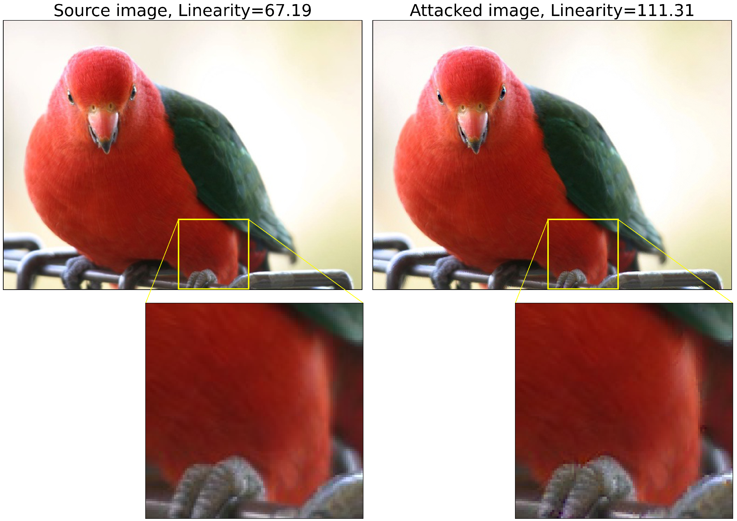
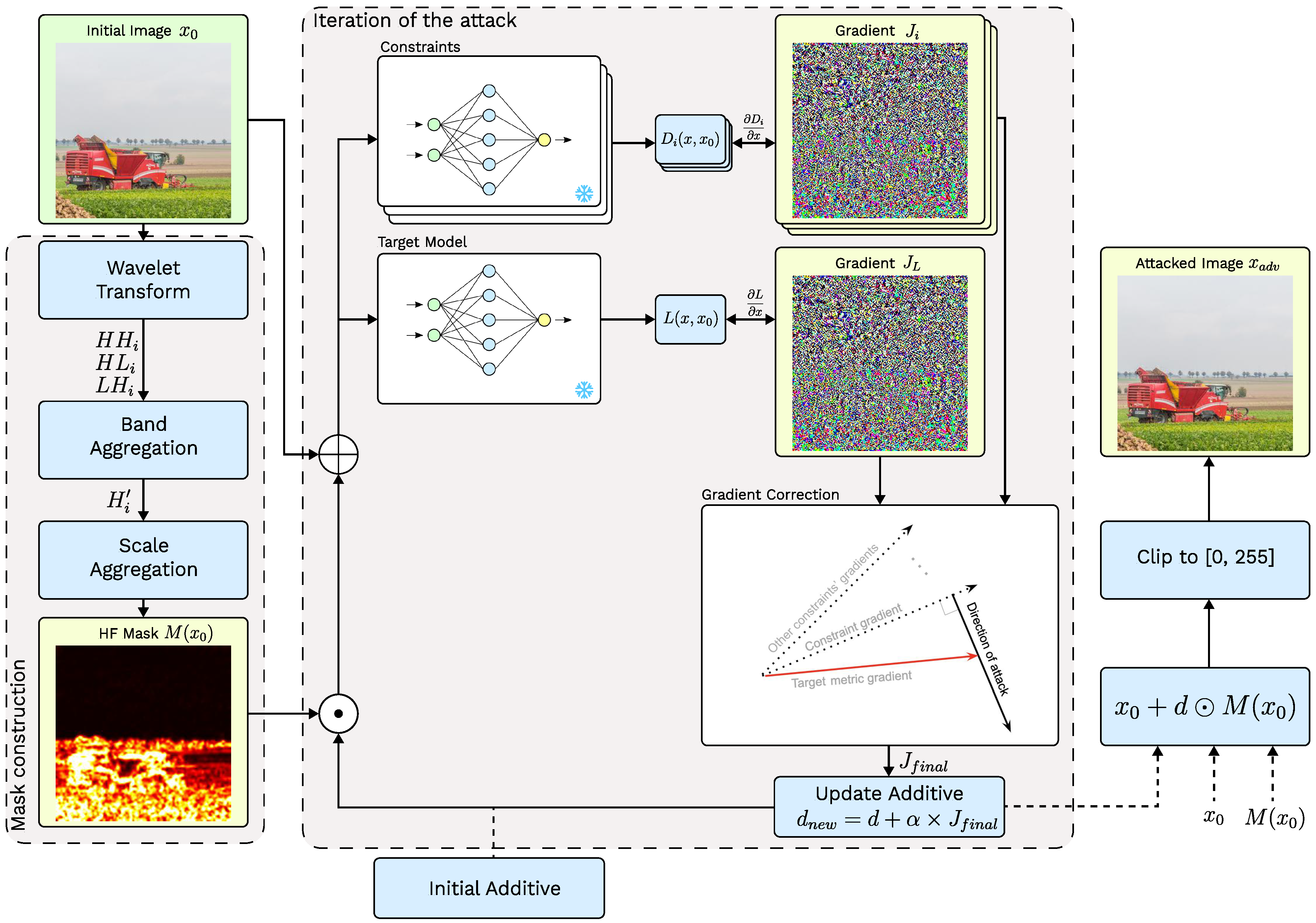

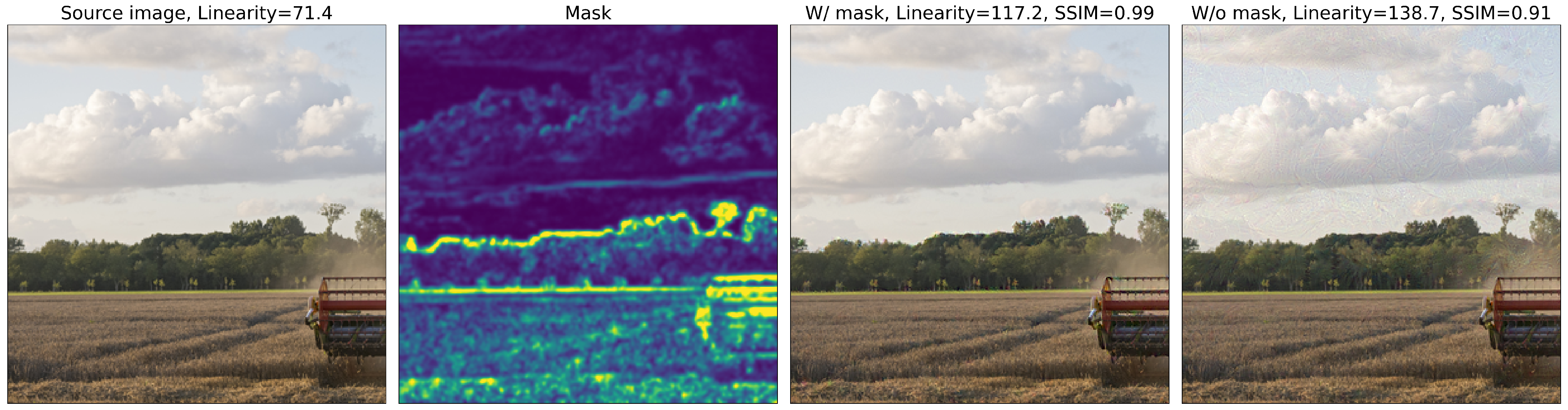
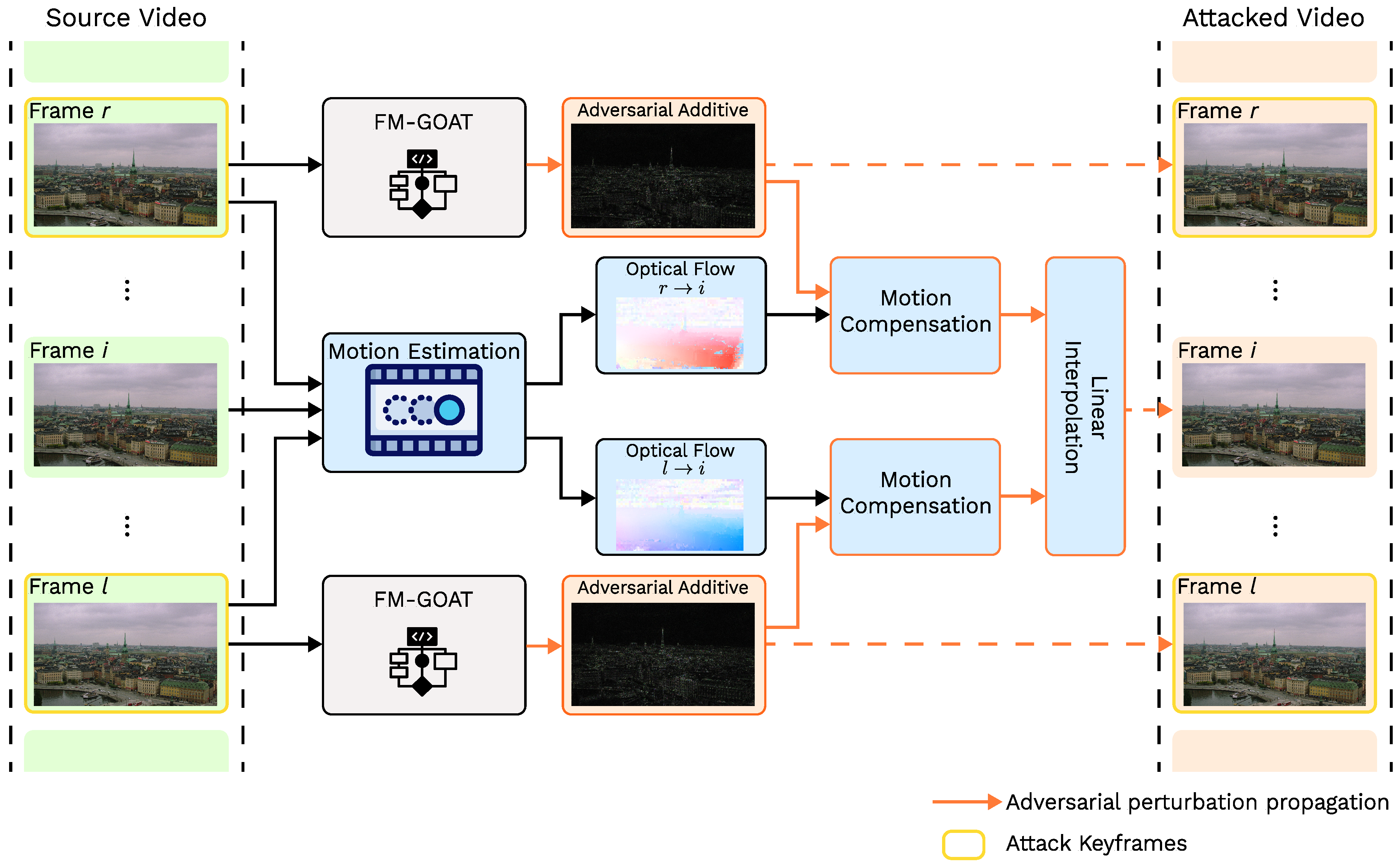
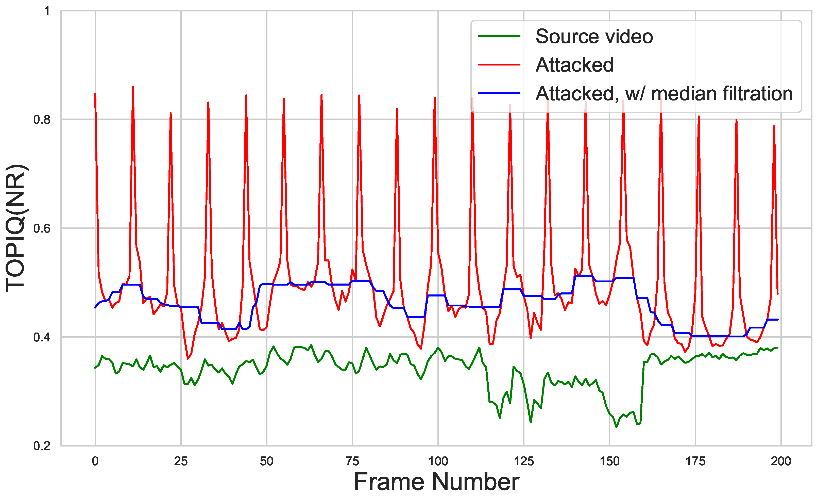
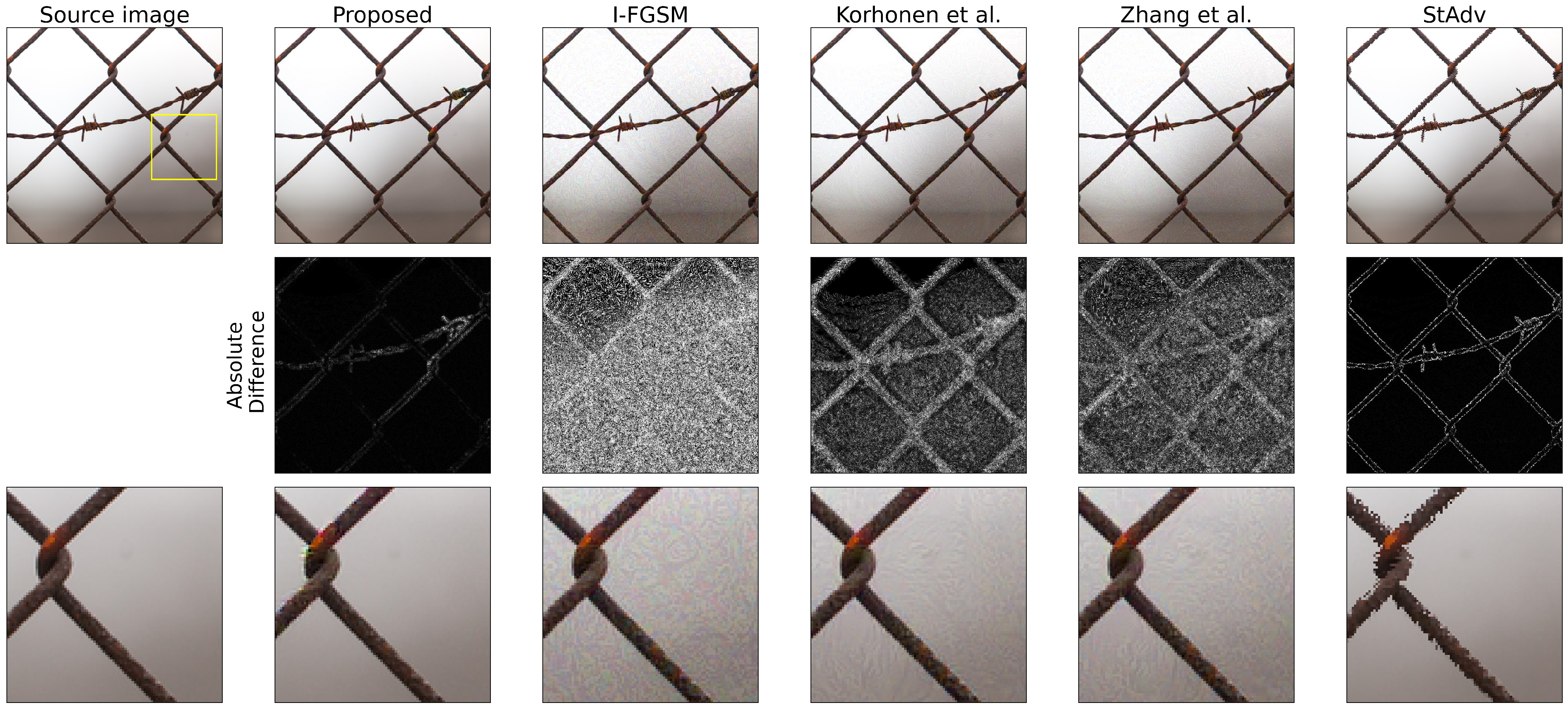


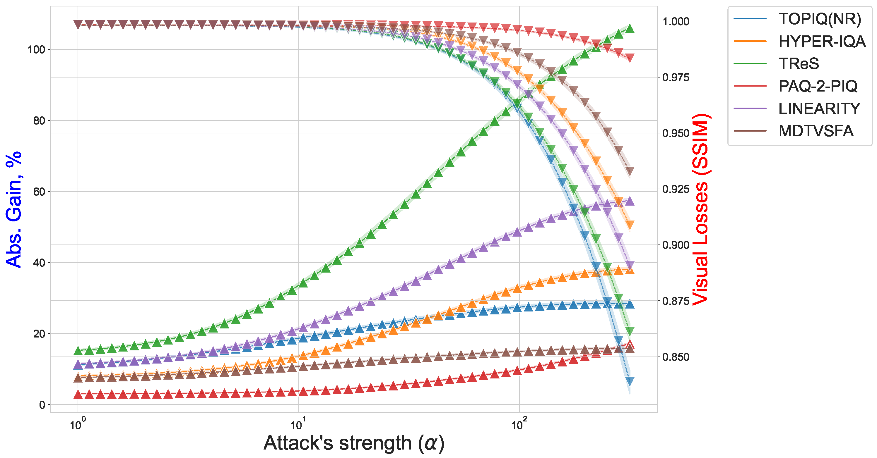
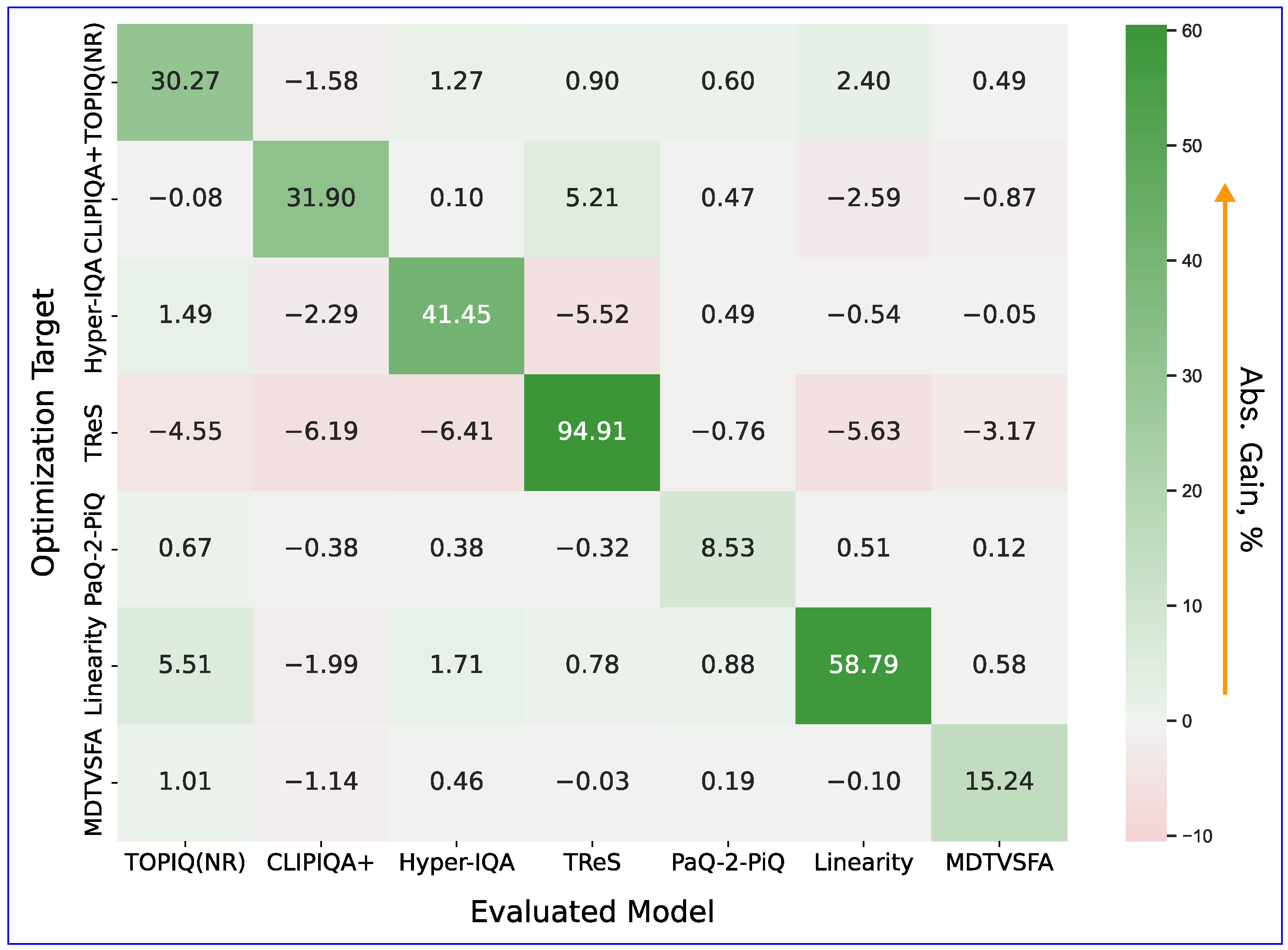
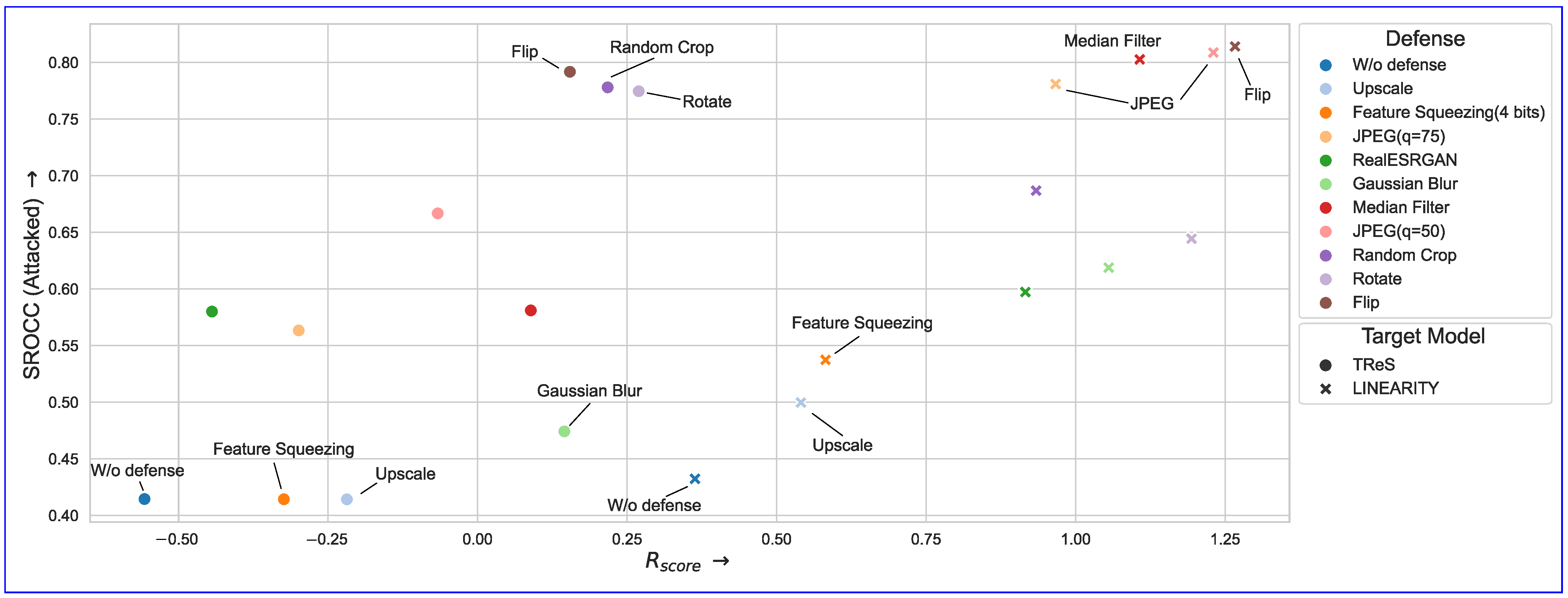
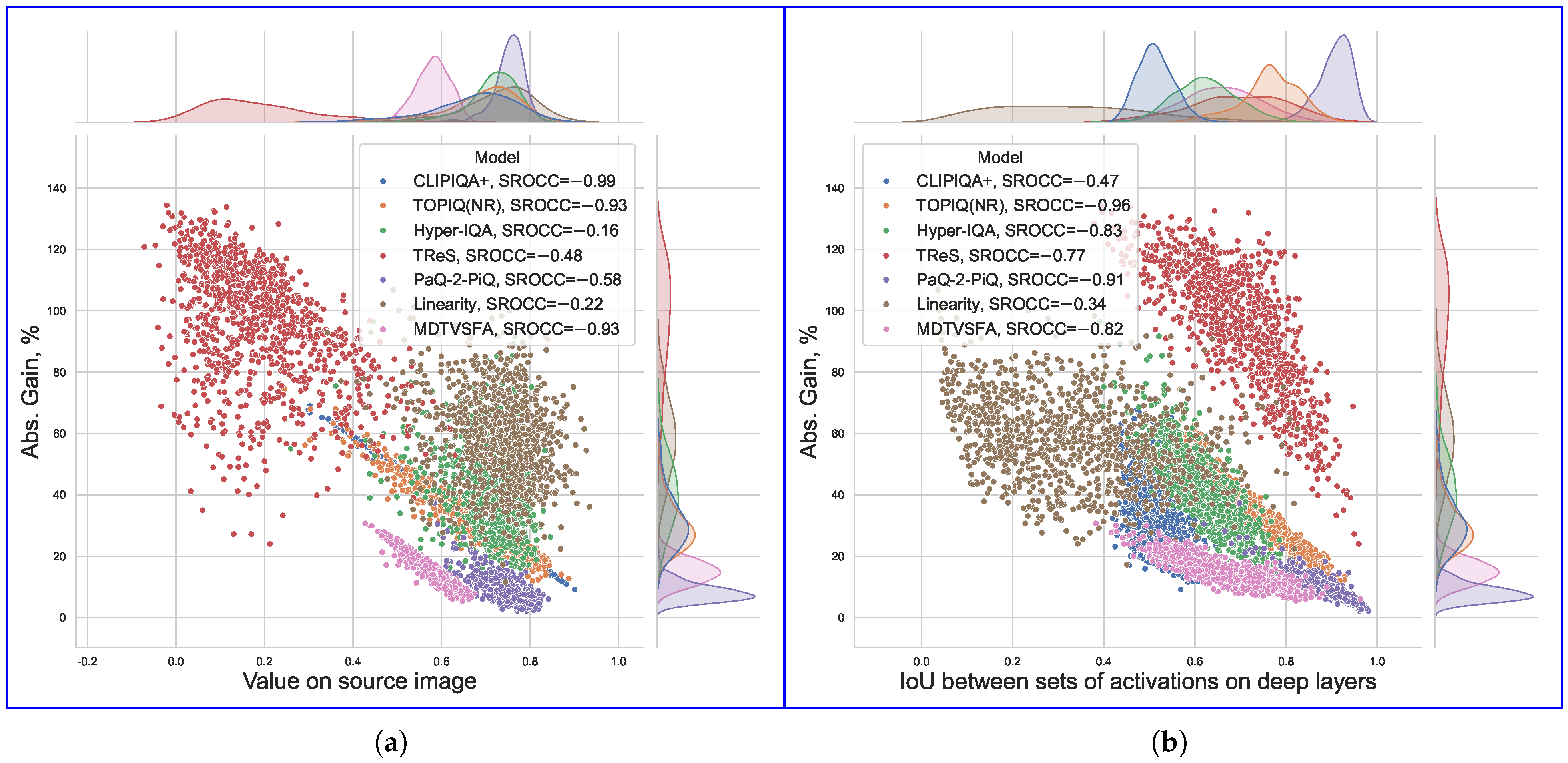
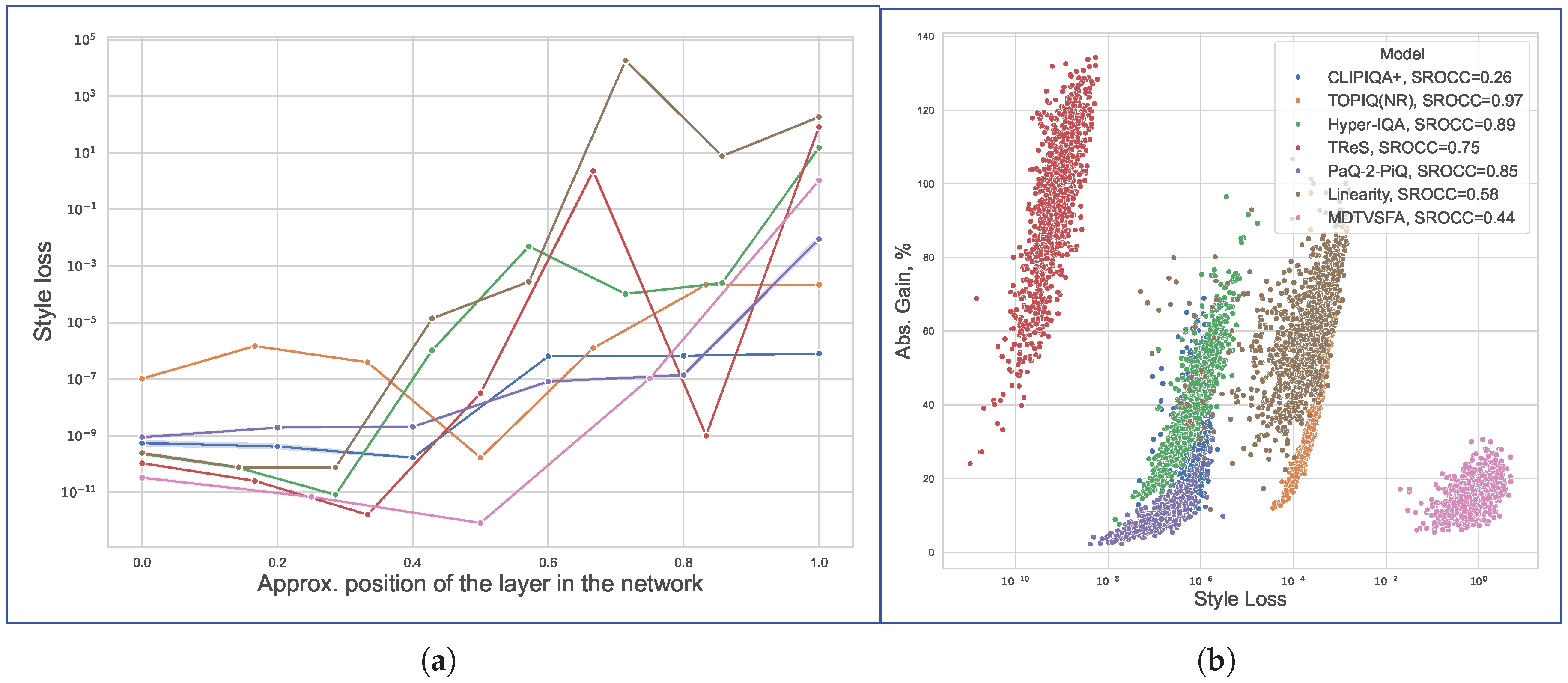
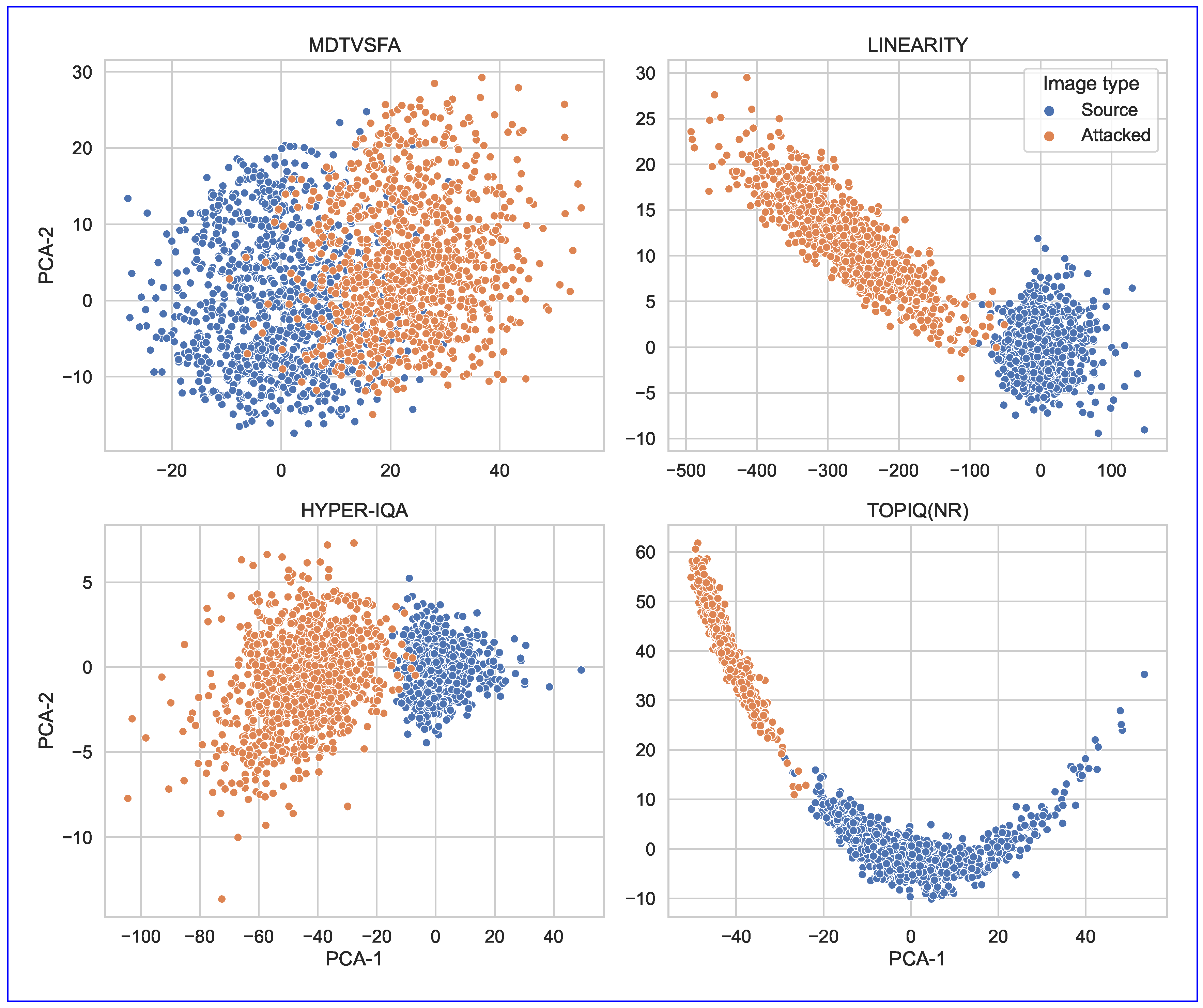

Disclaimer/Publisher’s Note: The statements, opinions and data contained in all publications are solely those of the individual author(s) and contributor(s) and not of MDPI and/or the editor(s). MDPI and/or the editor(s) disclaim responsibility for any injury to people or property resulting from any ideas, methods, instructions or products referred to in the content. |
© 2025 by the authors. Licensee MDPI, Basel, Switzerland. This article is an open access article distributed under the terms and conditions of the Creative Commons Attribution (CC BY) license (https://creativecommons.org/licenses/by/4.0/).