

Time Series Prediction Method of Clean Coal Ash Content in Dense Medium Separation Based on the Improved EMD-LSTM Model


 , ,
, ,
Abstract
1. Introduction
2. Literature Review
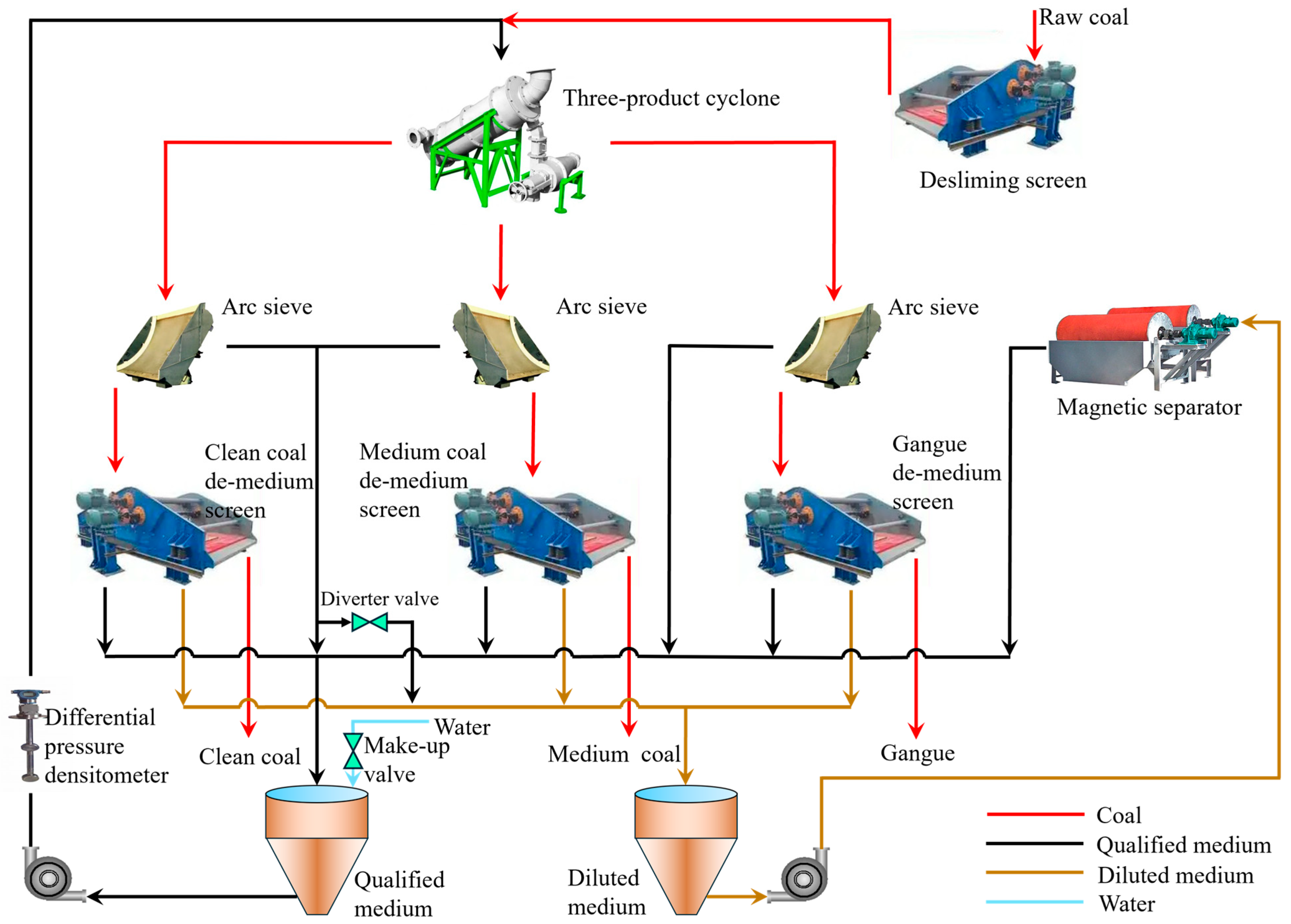
3. Research Methodology and Procedure
3.1. Research Methodology
3.1.1. EMD
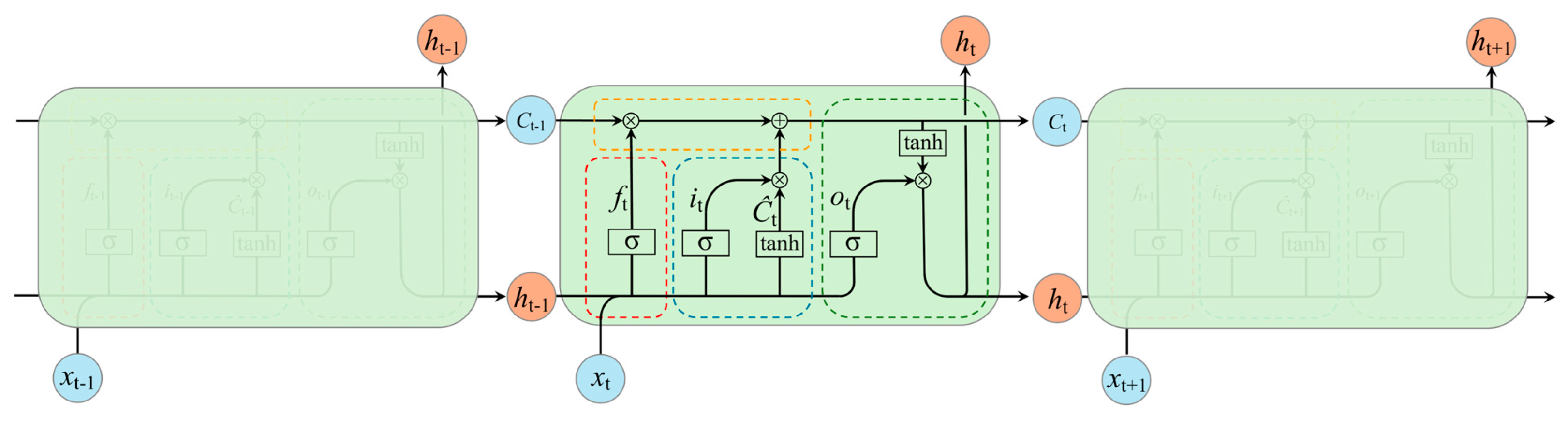
3.1.2. LSTM
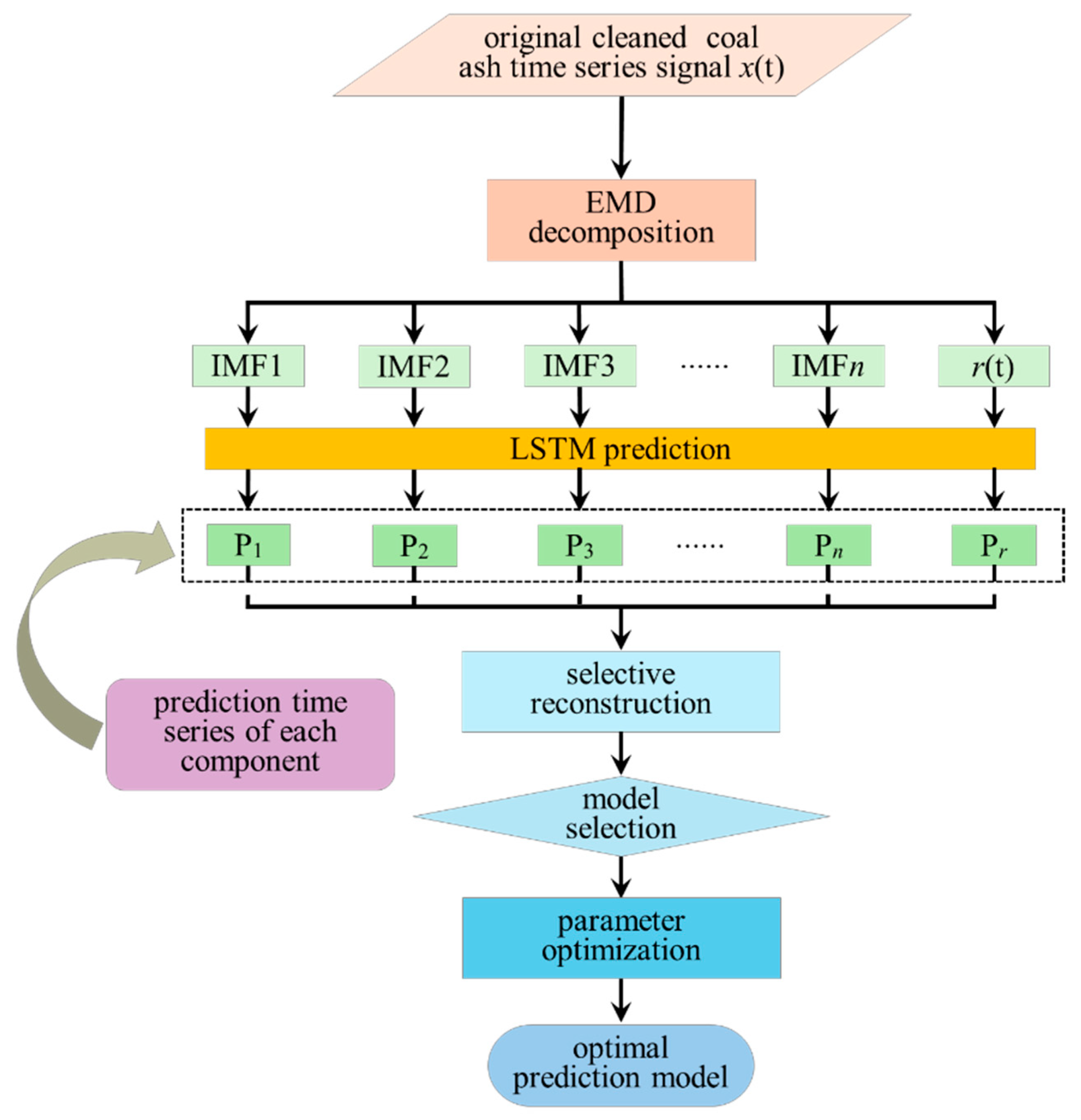
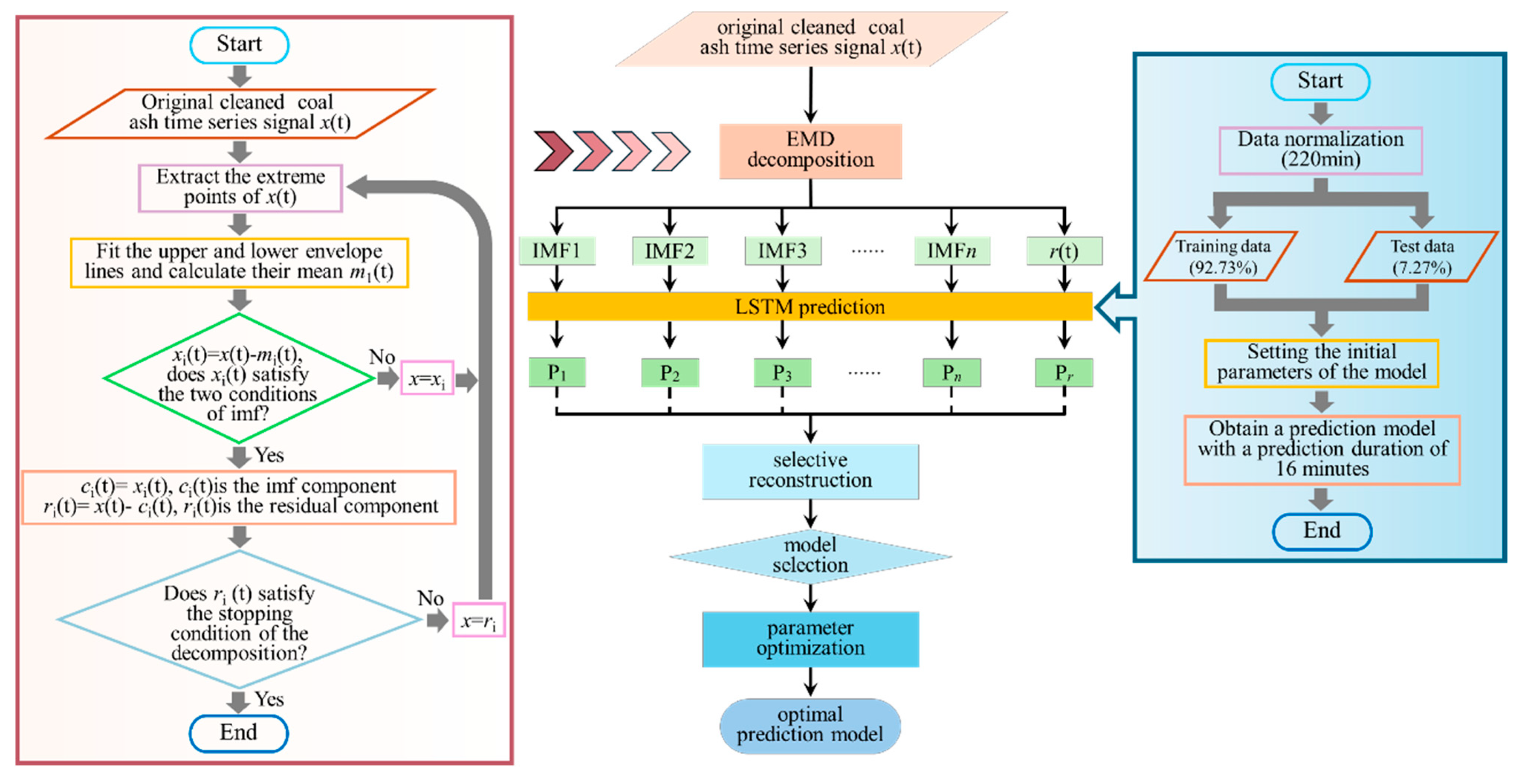
3.2. Framework of Prediction Methodology
3.3. Construction Process of Prediction Methodology
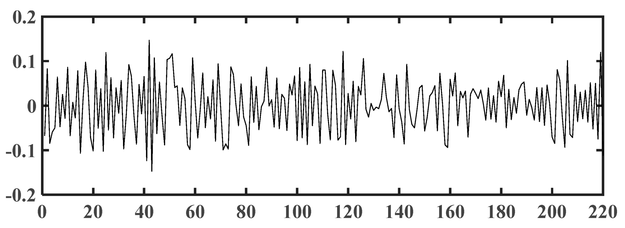
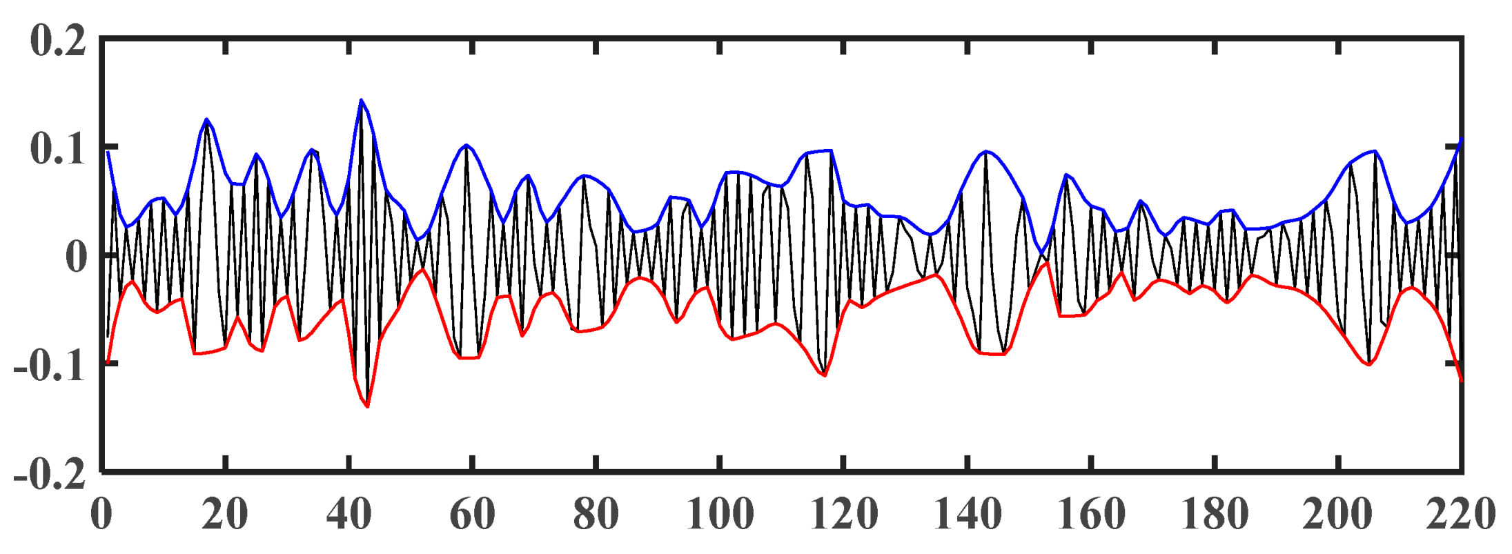
3.3.1. EMD of Time Series Signal
- (i)
- The number of extrema (sum of the number of maxima and minima) must be equal to or differ by at most one from the number of zero crossings.
- (ii)
- The mean of envelopes defined by the local maxima and minima should be zero at any point of the IMF.
3.3.2. LSTM Prediction for Each Component
3.3.3. Selective Reconstruction of Each Prediction Component
3.4. Structural Diagram of Prediction Methodology
4. Results and Analysis
4.1. Evaluation Metrics
4.2. EMD Results
4.3. LSTM Prediction of Time Series Component
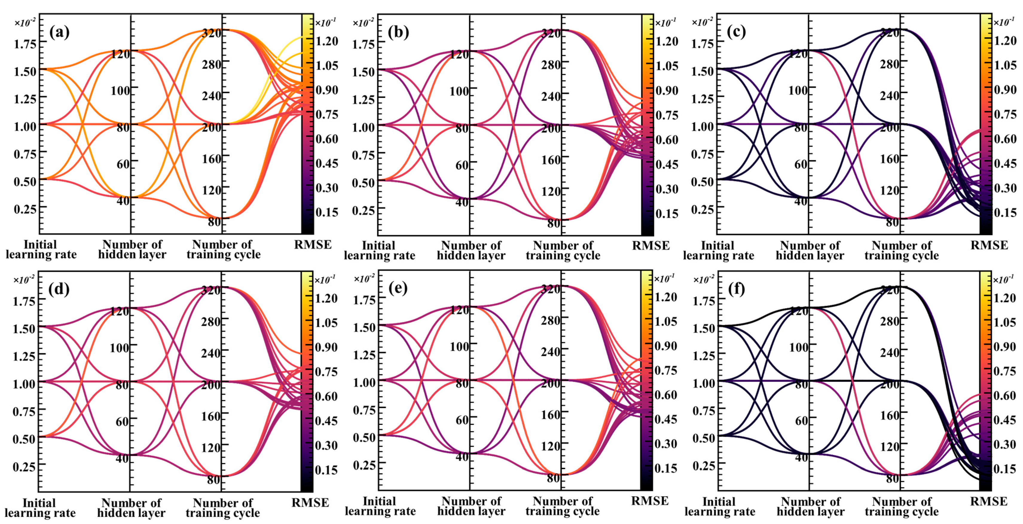
4.3.1. Experimental Setup
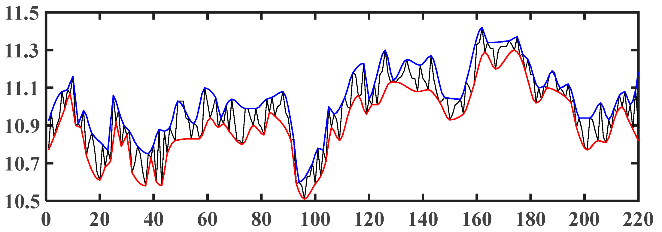
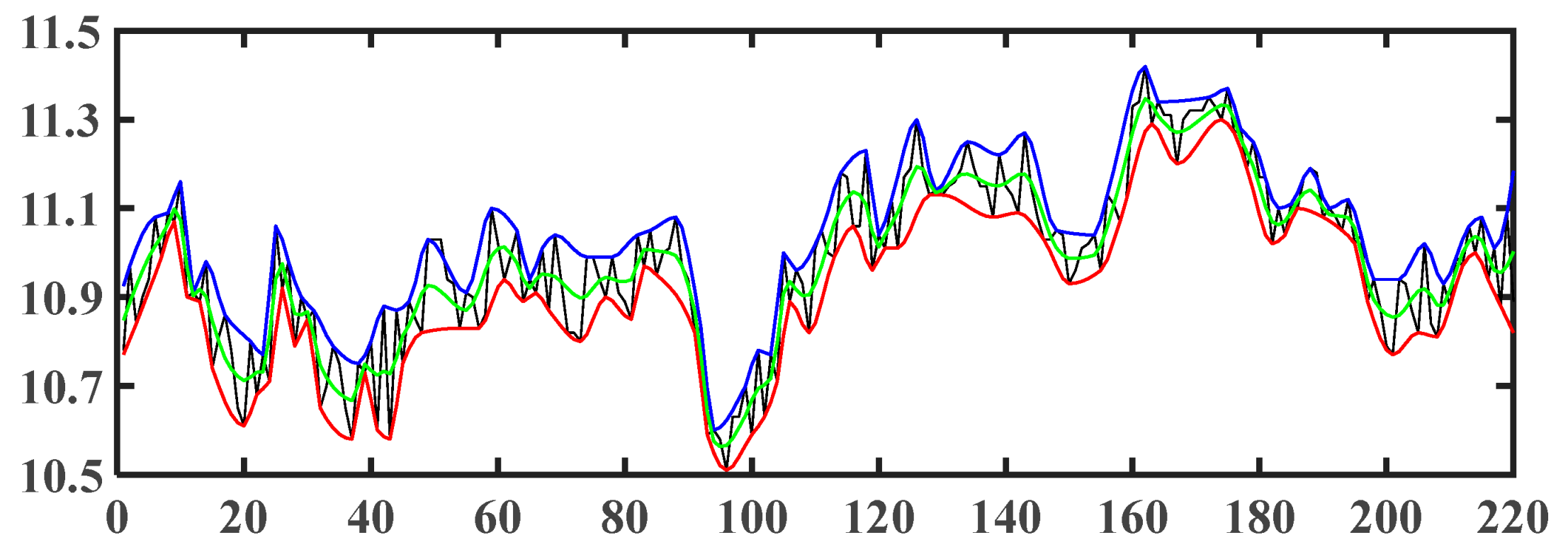
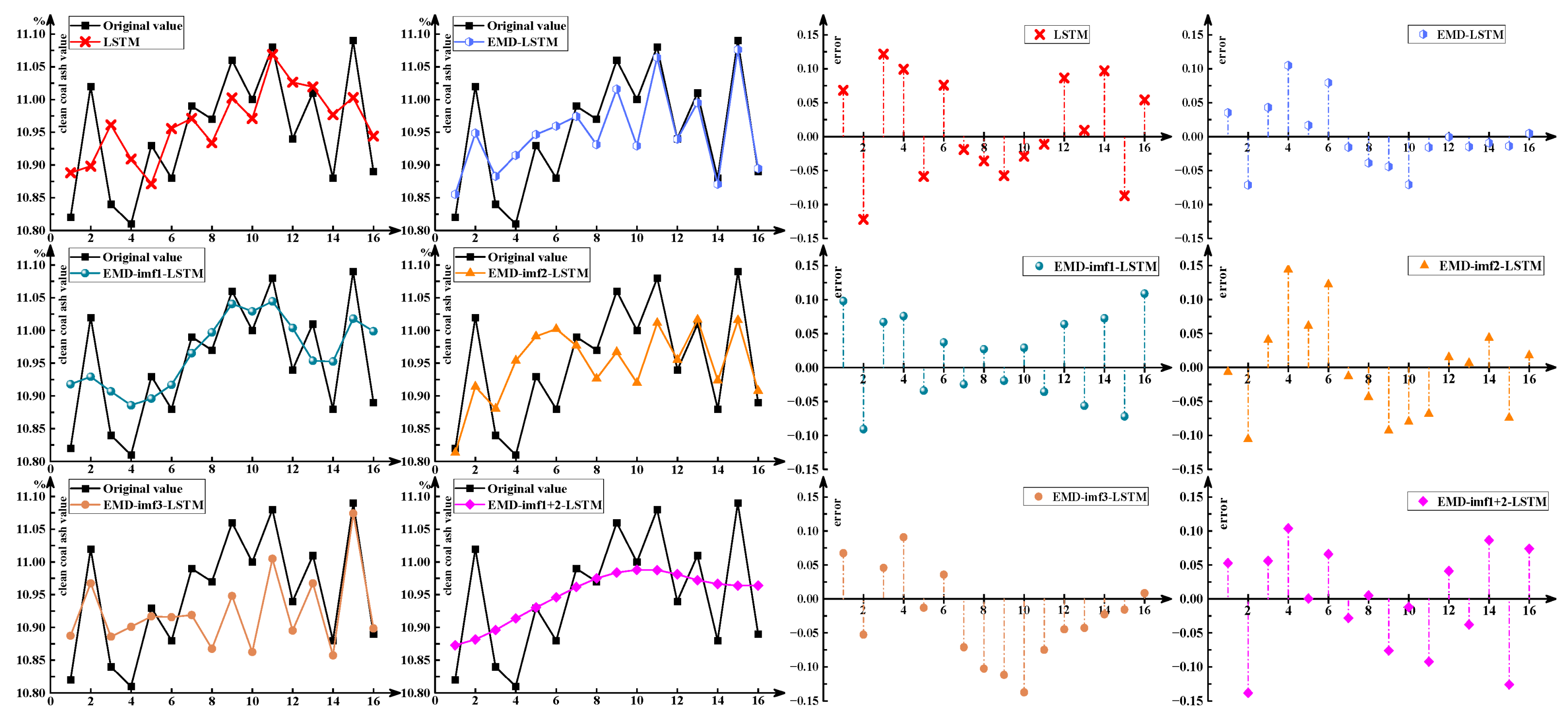
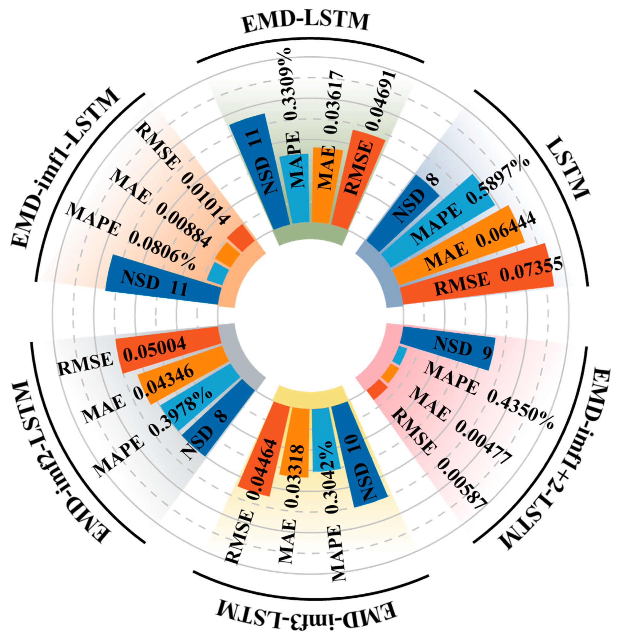
4.3.2. Prediction Results
- (1)
- Results of the error metric
- (2)
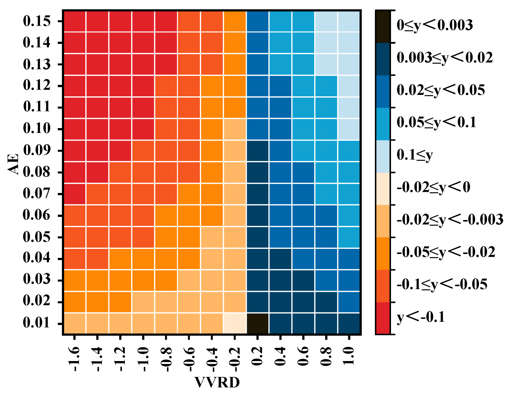
- Results of the VVRD metric
- (3)
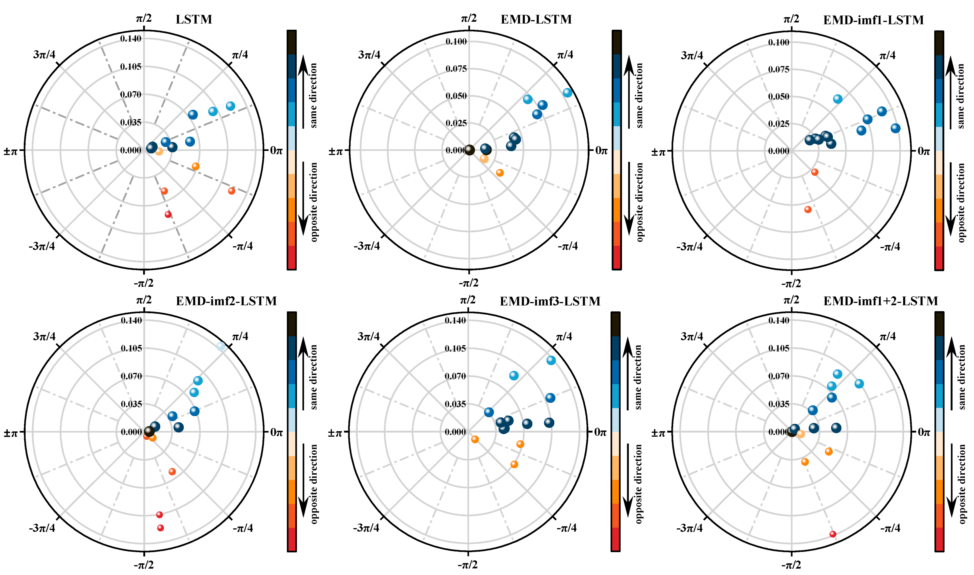
- Comprehensive results
4.4. Analysis of Model Selection
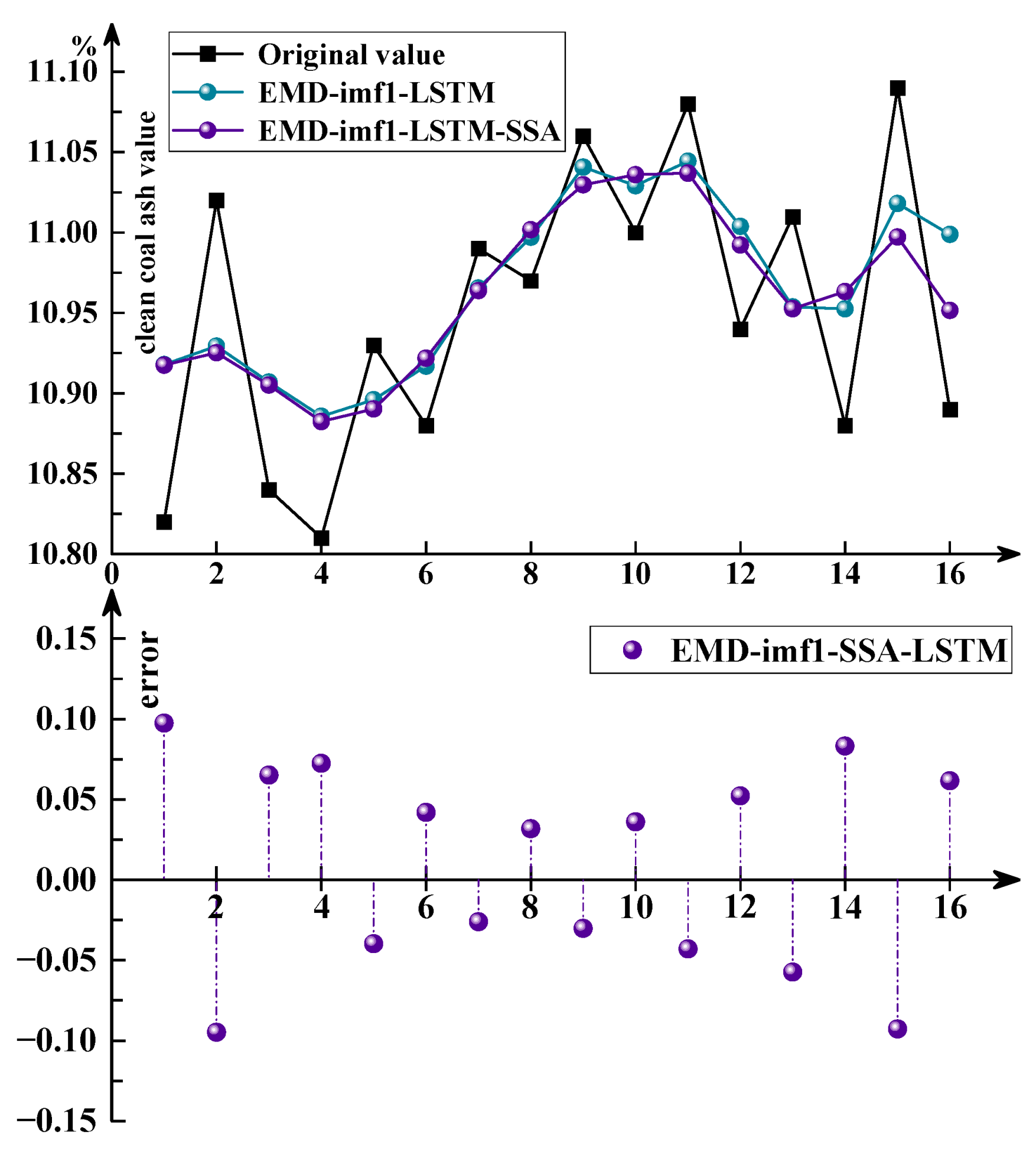
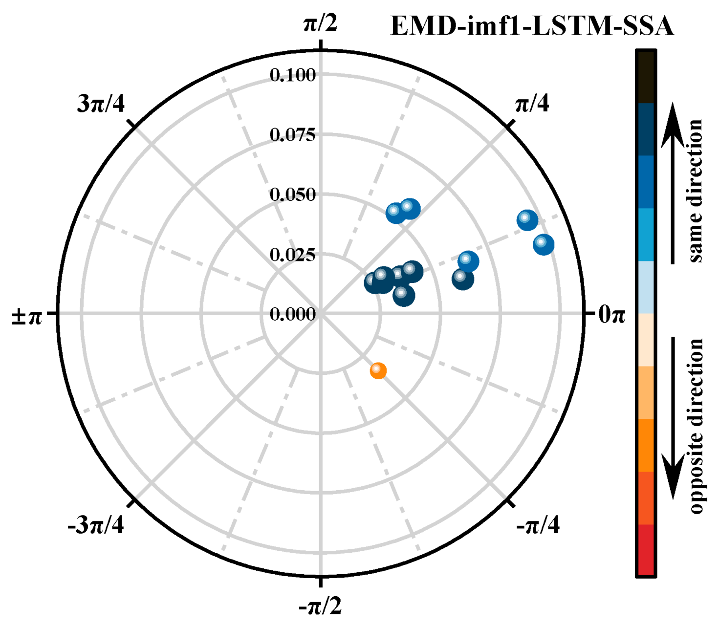
4.5. Parameter Optimization for the EMD-imf1-LSTM Model
5. Conclusions
Author Contributions
Funding
Data Availability Statement
Conflicts of Interest
References
- Zhang, B.; Zhu, G.Q.; Lv, B.; Yan, G.H. A novel and effective method for coal slime reduction of thermal coal processing. J. Clean. Prod. 2018, 198, 19–23. [Google Scholar] [CrossRef]
- Lv, W.; Wang, C. Intelligent control of heavy media separation. Int. J. Glob. Energy Issues 2023, 45, 86–100. [Google Scholar] [CrossRef]
- Tao, N.J.; Zheng, J.H.; Li, Z.Y. A General review of the course of development of China’s coal preparation technologies over the past five decades. Coal Prep. Technol. 2023, 51, 4047. (In Chinese) [Google Scholar] [CrossRef]
- Li, B.; Yu, X.; Zhang, K.; Yuan, Y.; Dou, N. Experimental study on ash reduction by classification flotation. Int. J. Coal Prep. Util. 2024, 4, 479–499. [Google Scholar] [CrossRef]
- Wang, G.H.; Kuang, Y.L.; Wang, Z.G.; Wang, Y.; Ji, L. A Real-Time Prediction Model for Production Index in Process of Dense-Medium Separation. Int. J. Coal Prep. Util. 2012, 32, 298–309. [Google Scholar] [CrossRef]
- Sriramoju, S.K.; Singh, R.; Sengupta, M.; Akhter, S.; Dash, P.S. Selective screening of coal to improve the washability characteristics at different levels of size reduction. Int. J. Coal Prep. Util. 2021, 42, 3070–3089. [Google Scholar] [CrossRef]
- Zhang, K.H.; Wang, W.D.; Lv, Z.Q.; Feng, J.D.; Li, H.X.; Zhang, C.L. LKDPNet: Large-Kernel Depthwise-Pointwise convolution neural network in estimating coal ash content via data augmentation. Appl. Soft Comput. 2023, 144, 110471. [Google Scholar] [CrossRef]
- Lu, F.C.; Liu, H.Z.; Lv, W.B. Deep correlation and precise prediction between static features of froth images and clean coal ash content in coal flotation: An investigation based on deep learning and maximum likelihood estimation. Measurement 2024, 224, 113843. [Google Scholar] [CrossRef]
- Cierpisz, S.; Heyduk, A. A simulation study of coal blending control using a fuzzy logic ash monitor. Control Eng. Pract. 2002, 10, 449–456. [Google Scholar] [CrossRef]
- Zhang, L.; Xia, X.; Zhu, B. A Dual-Loop Control System for Dense Medium Coal Washing Processes With Sampled and Delayed Measurements. IEEE Trans. Control Syst. Technol. 2017, 25, 2211–2218. [Google Scholar] [CrossRef]
- Theerayut, P.; Palot, S.; Chinawich, K.; Natatsawas, S.; Somthida, S.; Nutthakarn, P.; Onchanok, J.; Kreangkrai, M.; Apisit, N.; Ilhwan, P.; et al. Conventional and recent advances in gravity separation technologies for coal cleaning: A systematic and critical review. Heliyon 2023, 9, e13083. [Google Scholar] [CrossRef]
- Ma, L.C.; Wei, L.B.; Zhu, X.S.; Pei, X.Y.; Zhou, Q.F.; Liu, J.L. Response surface method for modeling of fine coal beneficiation by Knelson concentrator. Int. J. Coal Prep. Util. 2018, 41, 776–788. [Google Scholar] [CrossRef]
- Cui, Y.; Zhang, K.H.; Lv, Z.Q.; Li, H.X.; Song, S.; Zhang, C.L.; Wang, W.D.; Xu, Z.Q. Exploring the effect of various factors for ash content estimation via ensemble learning: Color-texture features, particle size, and magnification. Miner. Eng. 2023, 201, 108212. [Google Scholar] [CrossRef]
- Zhang, J.L.; Kang, W.Z.; Zhang, X.G.; Fan, C.J.; Lou, Y.Q. Discussion on ash prediction of cleaned coal in Taoshan Coal preparation Plant. Clean Coal Technol. 2007, 04, 15–17. (In Chinese) [Google Scholar] [CrossRef]
- Sun, X.L.; Cao, Z.G.; Yue, Y.H.; Kuang, Y.L.; Zhou, C.X. Online prediction of dense medium suspension density based on phase space reconstruction. Part. Sci. Technol. 2017, 36, 989–998. [Google Scholar] [CrossRef]
- Qiu, Z.Y.; Dou, D.Y.; Zhou, D.Y.; Yang, J.G. On-line prediction of clean coal ash content based on image analysis. Measurement 2021, 173, 108663. [Google Scholar] [CrossRef]
- Chen, P.; Wang, C.Y.; Wang, S.W.; Zhang, C.H.; Li, Z.W. Prediction of Cleaned Coal Yield and Partition Coefficient in Coal Gravity Separation Based on the Modified Hyperbolic Tangent Model. Min. Metall. Explor. 2022, 39, 2491–2502. [Google Scholar] [CrossRef]
- Zhang, Z.L.; Yang, J.G. Online Analysis of Coal Ash Content on a Moving Conveyor Belt by Machine Vision. Int. J. Coal Prep. Util. 2016, 37, 100–111. [Google Scholar] [CrossRef]
- Ali, D.; Hayat, M.B.; Lana, A.; Molatlhegi, O.K. An evaluation of machine learning and artificial intelligence models for predicting the flotation behavior of fine high-ash coal. Adv. Powder Technol. 2018, 29, 3493–3506. [Google Scholar] [CrossRef]
- Legnaioli, S.; Campanella, B.; Pagnotta, S.; Poggialini, F.; Palleschi, V. Determination of Ash Content of coal by Laser-Induced Breakdown Spectroscopy. Spectrochim. Acta Part B At. Spectrosc. 2019, 155, 23–126. [Google Scholar] [CrossRef]
- Yin, X.H.; Niu, Z.W.; He, Z.; Li, Z.J.; Lee, D.H. Ensemble deep learning based semi-supervised soft sensor modeling method and its application on quality prediction for coal preparation process. Adv. Eng. Inform. 2020, 46, 101136. [Google Scholar] [CrossRef]
- Zhou, C.X.; Sun, X.L.; Shen, Y.S.; Yue, Y.H.; Jing, M.Y.; Liang, W.N.; Zhang, H. Product quality prediction in dense medium coal preparation process based on recurrent neural network. Int. J. Coal Prep. Util. 2023, 44, 291–308. [Google Scholar] [CrossRef]
- Wang, J.; Wang, R.F.; Fu, X.; Wei, K.; Han, J.; Zhang, Q. Research on Dual GRU model driving by time series alignment for multi-step prediction of ash content of dense medium clean coal. Int. J. Coal Prep. Util. 2024, 44, 2200–2224. [Google Scholar] [CrossRef]
- Zhang, Y.T.; Li, C.L.; Jiang, Y.Q.; Sun, L.; Zhao, R.B.; Yan, K.F.; Wang, W.H. Accurate prediction of water quality in urban drainage network with integrated EMD-LSTM model. J. Clean. Prod. 2022, 354, 131724. [Google Scholar] [CrossRef]
- Ali, M.; Khan, D.M.; Alshanbari, H.M.; El-Bagoury, A.A. Prediction of Complex Stock Market Data Using an Improved Hybrid EMD-LSTM Model. Appl. Sci. 2023, 13, 1429. [Google Scholar] [CrossRef]
- Ghezaiel, W.; Ben Slimane, A.; Ben Braiek, E. Nonlinear multi-scale decomposition by EMD for Co-Channel speaker identification. Multimed. Tools Appl. 2017, 76, 20973–20988. [Google Scholar] [CrossRef]
- Xiong, Z.H.; Yao, J.J.; Huang, Y.M.; Yu, Z.X.; Liu, Y.L. A wind speed forecasting method based on EMD-MGM with switching QR loss function and novel subsequence superposition. Appl. Energy 2024, 353, 122248. [Google Scholar] [CrossRef]
- Rezaee, M.; Taraghi Osguei, A. Improving empirical mode decomposition for vibration signal analysis. Proceedings of the Institution of Mechanical Engineers. Part C J. Mech. Eng. Sci. 2017, 231, 2223–2234. [Google Scholar] [CrossRef]
- Sepp, H.; Jürgen, S. Long Short-Term Memory. Neural Comput. 1997, 9, 1735–1780. [Google Scholar]
- Pan, S.W.; Yang, B.; Wang, S.K.; Guo, Z.; Wang, L.; Liu, J.H.; Wu, S.Y. Oil well production prediction based on CNN-LSTM model with self-attention mechanism. Energy 2023, 284, 128701. [Google Scholar] [CrossRef]
- Yu, Y.; Si, X.S.; Hu, C.H.; Zhang, J.X. A Review of Recurrent Neural Networks: LSTM Cells and Network Architectures. Neural Comput. 2019, 31, 1235–1270. [Google Scholar] [CrossRef] [PubMed]
- Wei, Q.; Tan, C.D.; Gao, X.Y.; Guan, X.; Shi, X. Research on early warning model of electric submersible pump wells failure based on the fusion of physical constraints and data-driven approach. Geoenergy Sci. Eng. 2024, 233, 212489. [Google Scholar] [CrossRef]
- Huynh, A.N.L.; Deo, R.C.; Ali, M.; Abdulla, S.; Raj, N. Novel short-term solar radiation hybrid model: Long short-term memory network integrated with robust local mean decomposition. Appl. Energy 2021, 298, 117193. [Google Scholar] [CrossRef]
- Yu, R.G.; Gao, J.; Yu, M.; Lu, W.H.; Xu, T.Y.; Zhao, M.K.; Zhang, J.; Zhang, R.X.; Zhang, Z. LSTM-EFG for wind power forecasting based on sequential correlation features. Future Gener. Comput. Syst. 2019, 93, 33–42. [Google Scholar] [CrossRef]
- Hu, Y.T.; Zhang, Q. A hybrid CNN-LSTM machine learning model for rock mechanical parameters evaluation. Geoenergy Sci. Eng. 2023, 225, 211720. [Google Scholar] [CrossRef]
- Marcelo, A.C.; Gastón, S.; María, E.T. Improved complete ensemble EMD: A suitable tool for biomedical signal processing. Biomed. Signal Process. Control 2014, 14, 19–29. [Google Scholar] [CrossRef]
- Hadi, R.; Hamidreza, F.; Gholamreza, M. Stock price prediction using deep learning and frequency decomposition. Expert Syst. Appl. 2021, 169, 114332. [Google Scholar] [CrossRef]
- Fang, T.H.; Zheng, C.L.; Wang, D.H. Forecasting the crude oil prices with an EMD-ISBM-FNN model. Energy 2023, 263, 125407. [Google Scholar] [CrossRef]
- Smagulova, K.; James, A.P. A survey on LSTM memristive neural network architectures and applications. Eur. Phys. J. Spec. Top 2019, 228, 2313–2324. [Google Scholar] [CrossRef]
- Zhang, M.Z.; Jia, A.L.; Lei, Z.X. Inter-well reservoir parameter prediction based on LSTM-Attention network and sedimentary microfacies. Geoenergy Sci. Eng. 2024, 235, 212723. [Google Scholar] [CrossRef]
- Alex, S. Fundamentals of Recurrent Neural Network (RNN) and Long Short-Term Memory (LSTM) network. Phys. D Nonlinear Phenom. 2020, 404, 132306. [Google Scholar] [CrossRef]
- Zhou, F.T.; Huang, Z.H.; Zhang, C.H. Carbon price forecasting based on CEEMDAN and LSTM. Appl. Energy 2022, 311, 118601. [Google Scholar] [CrossRef]
- Gao, T.; Niu, D.X.; Ji, Z.S.; Sun, L.J. Mid-term electricity demand forecasting using improved variational mode decomposition and extreme learning machine optimized by sparrow search algorithm. Energy 2022, 261, 125328. [Google Scholar] [CrossRef]


| Frequency Band | Threshold | Range |
|---|---|---|
| Low Frequency | 10 30 | F ≤ 10 |
| Middle Frequency | 10 < F ≤ 30 | |
| High Frequency | 30 < F |
| Model | EMD-imf1-LSTM | EMD-imf1-LSTM-SSA | |
|---|---|---|---|
| Valuation Metrics | |||
| RMSE | 0.01014 | 0.0099389 | |
| MAE | 0.00884 | 0.0051748 | |
| MAPE | 0.0806% | 0.04720% | |
| NSD | 11 | 12 | |
Disclaimer/Publisher’s Note: The statements, opinions and data contained in all publications are solely those of the individual author(s) and contributor(s) and not of MDPI and/or the editor(s). MDPI and/or the editor(s) disclaim responsibility for any injury to people or property resulting from any ideas, methods, instructions or products referred to in the content. |
© 2025 by the authors. Licensee MDPI, Basel, Switzerland. This article is an open access article distributed under the terms and conditions of the Creative Commons Attribution (CC BY) license (https://creativecommons.org/licenses/by/4.0/).
Share and Cite
Cheng, K.; Zhang, X.; Zhou, K.; Zhou, C.; Li, J.; Yang, C.; Guo, Y.; Wang, R. Time Series Prediction Method of Clean Coal Ash Content in Dense Medium Separation Based on the Improved EMD-LSTM Model. Big Data Cogn. Comput. 2025, 9, 159. https://doi.org/10.3390/bdcc9060159
Cheng K, Zhang X, Zhou K, Zhou C, Li J, Yang C, Guo Y, Wang R. Time Series Prediction Method of Clean Coal Ash Content in Dense Medium Separation Based on the Improved EMD-LSTM Model. Big Data and Cognitive Computing. 2025; 9(6):159. https://doi.org/10.3390/bdcc9060159
Chicago/Turabian StyleCheng, Kai, Xiaokang Zhang, Keping Zhou, Chenao Zhou, Jielin Li, Chun Yang, Yurong Guo, and Ranfeng Wang. 2025. "Time Series Prediction Method of Clean Coal Ash Content in Dense Medium Separation Based on the Improved EMD-LSTM Model" Big Data and Cognitive Computing 9, no. 6: 159. https://doi.org/10.3390/bdcc9060159
APA StyleCheng, K., Zhang, X., Zhou, K., Zhou, C., Li, J., Yang, C., Guo, Y., & Wang, R. (2025). Time Series Prediction Method of Clean Coal Ash Content in Dense Medium Separation Based on the Improved EMD-LSTM Model. Big Data and Cognitive Computing, 9(6), 159. https://doi.org/10.3390/bdcc9060159