FAD-Net: Automated Framework for Steel Surface Defect Detection in Urban Infrastructure Health Monitoring

Abstract

Steel plays a fundamental role in modern smart city development, where its surface structural integrity is decisive for operational safety and long-term sustainability. While deep learning approaches show promise, their effectiveness remains limited by inadequate receptive field adaptability, suboptimal feature fusion strategies, and insufficient sensitivity to small defects. To overcome these limitations, we propose FAD-Net, a deep learning framework specifically designed for surface defect detection in steel materials within urban infrastructure. The network incorporates three key innovations: The RFCAConv module, which leverages dynamic receptive field construction and coordinate attention mechanisms to enhance feature representation for defects with long-range spatial dependencies and low-contrast characteristics. The MSDFConv module, employing multi-scale dilated convolutions with optimized dilation rates to preserve fine details while expanding the receptive field. An Auxiliary Head that introduces hierarchical supervision to improve the detection of small-scale defects. Experiments on the GC10-DET dataset showed that FAD-Net achieved 5.0% higher mAP@0.5 than baseline models. Cross-dataset validation with NEU and RDD2022 further confirmed its robustness. These results demonstrate FAD-Net’s effectiveness for automated infrastructure health monitoring.

1. Introduction

Steel, as the fundamental material for modern urban infrastructure, plays a decisive role in ensuring the structural safety of critical facilities such as bridges and tunnels. During steel manufacturing processes, surface defects inevitably emerge due to rolling parameter variations and non-uniform heating conditions. These production-induced defects subsequently become potential structural weak points when the material enters service, ultimately compromising the long-term reliability of urban infrastructure [1,2]. Characteristic surface defect categories in steel materials include Crease, Waist folding, Silkspot, Water spot, Punching, and Inclusion, as shown in Figure 1. These defects are often complex, with irregular shapes and long-range spatial dependencies, and some are even highly similar to the texture or color of the steel. Moreover, these defects vary widely in size and morphology. Small defects, such as Punching and Inclusion, are easily overlooked but can gradually develop into more serious problems over time.

Traditional manual visual inspection for steel surface defect detection is inefficient and subjective. With the rapid development of machine vision [3] and deep learning [4], image-based steel surface defect detection methods have been widely studied and applied. Machine vision, a powerful tool enabled by computer vision technology, enables the automatic detection of steel surface defects [5]. Deep learning methods can automatically extract high-level features from raw images, significantly improving detection accuracy and efficiency. However, current detection technologies suffer from high false detection and miss rates, making the improvement of algorithm accuracy and stability a key challenge [6,7].

Computer vision, a fundamental and challenging area in AI, has gained recent attention. Algorithm performance is typically evaluated based on accuracy and speed. With the fast progress of deep learning, deep-learning-based object detection has become mainstream. Currently, there are two main types of object detectors: two-stage regional detectors like the R-CNN [8] series and one-stage regression-based detectors like the YOLO series. Computer vision-based methods are now used in many real-world applications, such as defect inspection, autonomous driving, and medical imaging. The YOLO series [9,10,11,12,13,14,15,16], able to predict all objects in an image via a single forward pass, stands out among object detection algorithms due to its speed–accuracy balance [17]. Since its introduction, YOLO has evolved through several versions, each building on previous ones to address limitations and enhance performance. YOLO11, the latest version and a SOTA detector in object detection, is celebrated for its fast and stable detection. But YOLO11 still has shortcomings in handling complex steel surface defects. To address these issues, we present an optimized FAD-Net (Fusion-Aware Detection Network), which makes significant contributions in three key aspects:

• Traditional convolution operations are limited by a fixed receptive field, which restricts the ability to capture both global features and detailed information in complex defect patterns. This paper introduces the RFCAConv (Receptive Field and Coordinate Attention Convolution) module, which combines the advantages of coordinate attention for spatial modeling with a dynamic receptive field construction strategy. By employing a non-parametric shared convolution structure, it reduces feature overlap and information loss, improving the model’s ability to capture long-range spatial dependencies and enhancing its ability to detect low-contrast defects.
• In Feature Pyramid Networks (FPNs), traditional pyramid pooling can result in the loss of detailed information, especially when handling multi-scale defects. This paper proposes the MSDFConv (Multi-Scale Dilated Fusion Convolution) module, which uses stacked dilated convolutions instead of pooling to expand the receptive field, preserving detailed features while improving the model’s ability to detect defects at different scales.
• Existing algorithms struggle with small target detection, especially when dealing with small defects on steel surfaces, often leading to missed detections. Therefore, this paper introduces the Auxiliary Head, which introduces additional supervisory signals at the intermediate layers of the network. Through multi-level feature fusion, it increases the network’s sensitivity to small defects.

The rest of this paper is organized as follows: Section 2 reviews the research progress in the field of defect detection; Section 3 introduces the main principles of the proposed algorithm; Section 4 analyzes the experimental results and data; Section 5 concludes the paper and discusses future directions.

2. Related Work

Surface defect inspection of steel materials is critical for ensuring the safety and durability of key structures like bridges and tunnels in urban infrastructure [1]. Existing steel surface defect detection methods are categorized into four types: structure-based, statistical-based, filtering-based, and learning-based [18].

Structure-based methods identify defects by extracting texture primitives and characterizing image regions according to their placement rules. For example, Zhang et al. [19] used an adaptive thresholding and morphological reconstruction approach for detecting defects in aluminum alloy wheels. Shi et al. [20] improved the Sobel edge detection algorithm to reduce noise impact and achieve more precise defect localization. However, the accuracy of this method is limited when detecting low-contrast defects. Liu et al. [21] proposed a mathematical morphology-based enhancement operator (EOBMM) to address uneven illumination in steel strip defect images and enhance image details. However, this method has high computational complexity when dealing with multi-scale defects. Statistical-based methods describe texture features using the grayscale distribution of image regions, and common techniques include histograms, co-occurrence matrices, and local binary patterns. For instance, Aminzadeh M et al. [22] presented a thresholding method for defect identification based on histogram information. While histogram methods have been used in modeling and visualization, the information they can extract is limited. Yan K et al. [23] enhanced the LBP method by introducing the Complete Local Ternary Pattern (CLTP) to detect welds, improving performance across different scenarios such as varying lighting conditions. Nevertheless, LBP-based methods remain sensitive to noise and directional information and are prone to interference from complex backgrounds.

Filtering-based methods analyze images as 2D signals using techniques like curvelet transforms, Gabor filters, and wavelet transforms. For example, Cong et al. [24] used Gabor filters to extract texture features of surface defects in steel strips, determining optimal filter parameters by maximizing an evaluation function that quantified the energy response difference between defective and non-defective images. Wu et al. [25] decomposed surface defect images of hot-rolled steel plates into 40 components across five scales and eight directions using Gabor wavelets. They extracted the mean and variance of the real and imaginary parts for each component and the original image, forming a 162-dimensional feature vector. However, these methods have high computational complexity due to localized analysis in both spatial and frequency domains, making it challenging to meet real-time detection requirements.

With the advancement of computational power and deep learning technologies, deep learning-based methods have gradually become mainstream in steel strip surface defect detection. These methods can automatically learn feature representations without manual feature extraction rule design, and they offer stronger representation and adaptability. Current deep learning-based defect detection methods are mainly divided into single-stage and two-stage algorithms. Two-stage algorithms first extract candidate boxes from an image and then refine the detection results based on the candidate regions. For example, Zhao et al. [26] proposed a transmission line insulator identification and fault detection model based on improved Faster R-CNN. This model integrates feature pyramid networks (FPNs) to enhance insulator detection in complex background images and employs an HSV color space adaptive threshold algorithm for image segmentation to mitigate the effects of lighting, background noise, and shooting angles. Liu et al. [27] proposed a multi-scale context detection network (MSC-DNet) that introduces auxiliary image-level supervision (AIS) to enhance defect-distinguishing features, achieving excellent performance in complex backgrounds. However, two-stage detection models have high computational complexity, making it difficult to meet real-time detection requirements. Single-stage algorithms directly compute results from images and are fast. For example, Wu et al. [28] proposed a lightweight feature fusion method based on YOLOv3, enabling the detection network to operate on single-scale feature maps and reducing computational complexity. Nevertheless, its adaptability to different materials and textures is limited, especially in complex steel surface textures and multi-scale defect scenarios. Zhang et al. [29] proposed CrackNet, which eliminates pooling layers to maintain original image resolution and uses feature extractors to generate multi-directional and multi-scale feature maps. Yin et al. [30] developed an automatic sewer pipeline defect detection framework based on YOLOv3, employing a three-scale prediction method to identify defects of various sizes. Zhao et al. [31] proposed an improved RDD-YOLO model based on YOLOv5, integrating Res2Net as the backbone network, dual feature pyramid networks, and a decoupled head structure, achieving a balance between detection accuracy and real-time performance. However, this model still has limitations in fine-grained feature extraction and the accurate identification of complex defects.

Although existing research has made significant progress in steel defect detection for urban infrastructure, current methods still have obvious limitations in handling the unique texture characteristics and complex shape variations of construction steel surfaces. They also struggle to meet the low computational complexity requirements of real-time monitoring scenarios. This study proposes a surface defect detection model specifically designed for construction steel materials, offering a reliable solution for the intelligent safety maintenance of urban infrastructure [32].

3. Methods

To tackle the challenges of long-range saptial dependencies, low contrast in some defects, significant scale differences, diverse defect shapes, and limited small target detection capabilities on steel surfaces, we propose the FAD-Net model. To enhance the model’s ability to recognize long-range, complex defects and improve the representation of defect region features, we introduce the RFCAConv module, which replaces the conventional convolutional modules in the network architecture as well as those in the C3k2 feature extraction module. This module applies the CA mechanism to the receptive field’ s spatial features, focusing on regions with significant information, and uses them in place of standard convolution operations. To address the issue of local detail loss caused by pooling in traditional spatial pyramid pooling operations, we propose the MSDFConv module to replace the spatial pooling pyramid module. This module captures multi-scale information by stacking convolutions with varying dilation rates and uses a shared convolution kernel design to reduce computational complexity. Finally, we propose the Auxiliary Head. By integrating multi-scale feature learning modules P3, P4, and P5 and incorporating a larger positive sample allocation strategy (top-K = 13) and a dynamic task alignment allocator (Task-Aligned Assigner), this model effectively enhances the network’s sensitivity to small defects, thereby improving detection completeness.

The architecture of the FAD-Net network is illustrated in Figure 2.

3.1. RFCAConv

Steel surfaces exhibit unique defect distribution patterns. Some defects span the entire width or concentrate at edges, featuring complex shapes and long-range spatial dependence. Additionally, low-contrast defects possess textural features highly similar to the background, significantly increasing detection difficulty. Conventional convolutional operations, due to their parameter-sharing mechanism, cannot capture differences in information from various positions. Although existing spatial attention mechanisms enhance model focus on key areas by adjusting feature weight distributions, the issue of shared attention weights persists. To address these challenges, this paper proposes an innovative RFCAConv module that combines dynamic receptive field strategies with a CA [33] mechanism.

In the RFCAConv module, as illustrated in Figure 3, the input feature map X first undergoes a set of 3 × 3 group convolutions, increasing the number of channels ninefold. The feature map is then reshaped into a C × 3H × 3W receptive field spatial feature map. This rearrangement expands each point in the original feature map into a 3 × 3 matrix, thereby significantly enriching the feature information across different spatial locations. Subsequently, average pooling operations are performed on the receptive field spatial feature map along the H and W dimensions to aggregate global information within the receptive field. The features from these two dimensions are stacked, and a 1 × 1 convolution is applied to facilitate information exchange among channels. This step reduces redundancy among channels and enhances feature representation.

The aggregated feature vector is divided into two parts, corresponding to the height and width information of the receptive field spatial feature map. Separate 1 × 1 convolution operations are performed on these two parts to independently generate attention weight matrices for height and width. The attention weights in both the height and width directions are element-wise multiplied with the receptive field spatial feature map. This operation enhances key regional information within the feature map while suppressing irrelevant areas. When detecting distant defects, dynamic weights place greater emphasis on the defect’s extension direction, enabling the model to better capture long-range dependent defects. For low-contrast defects, the model focuses on local minute features, significantly improving detection accuracy.

Finally, a 3 × 3 convolutional layer with a stride of 3 is employed to restore the spatial dimensions of the feature map to match the original input, ensuring seamless integration with subsequent network layers. In the network implementation, all standard convolutional modules in the backbone and neck networks are replaced by RFCAConv modules. Within the C3k2 Bottleneck structure, the RFCAConv module replaces the second standard convolutional module. The detailed structure of the improved C3k2_RFCAConv is depicted in Figure 4.

3.2. MSDFConv

The surface of construction steels exhibits distinct multi-scale characteristics. Traditional multi-scale feature extraction and fusion modules employ fixed-size pooling windows to integrate information across different scales. While this approach mitigates scale differences to some extent, it falls short in capturing detailed features. Moreover, the fixed window size restricts the expansion of the receptive field, hindering the balance between local details and global context.

To address these limitations, we propose the MSDFConv module, which incorporates dilated convolutions with varying dilation rates within the convolutional layers. This approach enables feature extraction across different scales, which is highly beneficial for capturing objects of varying sizes and contextual information within images. Specifically, convolutional layers with lower dilation rates excel at capturing fine local details such as edges and textures. In contrast, those with higher dilation rates perform better in capturing the global context, including the relative positions of objects and background information.

In order to boost the efficiency of the model and reduce redundancy, we implemented Shared Convolutional Layers (ShareConv). This approach reduces the number of parameters by sharing the weights of the convolutional kernel $W_{share}$.

As shown in Figure 5, the input feature map X is first transformed by a 1 × 1 convolution, which reduces the number of channels to a hidden dimension $C_{hid}$, producing the feature map $Y_0$:

$$Y_0=Conv(X,W_{conv})$$

(1)

Then, for each dilation rate $r\in r_1,r_2,\dots ,r_n$, the shared convolutional kernel weights $W_{share}$ are applied to the previous feature map $Y_{i-1}$ to generate a new feature map $Y_i$:

$$Y_i=Conv(Y_{i-1},W_{share},dilation=r)$$

(2)

To ensure the size consistency of input and output feature maps, dynamic padding adjustments are applied to each dilated convolution layer, ensuring a smooth transition between convolutions with different dilation rates, and the calculation formula is as follows:

$$p=⌊{\displaystyle \frac{(k-1)·r}{2}}⌋$$

(3)

Finally, all the feature maps $Y_0,Y_1,\dots ,Y_n$ are concatenated, and a 1 × 1 convolution is applied to adjust the channel dimensions of the concatenated feature maps, resulting in the final output feature map:

$$Output=Conv(Concat(Y_0,Y_1,\dots ,Y_n),W_{final})$$

(4)

Through parameter-sharing and multi-scale feature extraction, the model maintains its performance while achieving greater computational efficiency.

3.3. Auxiliary Head

Surfaces of steel materials in urban infrastructure often exhibit minute surface anomalies. Although dilated convolutions expand the receptive field and effectively prevent detail loss from traditional pooling operations, larger dilation rates may still overlook high-resolution details. To address this issue, we introduced an Auxiliary Head into the baseline detection framework. By adding extra loss terms to intermediate feature maps, the network is guided to enhance sensitivity to small-scale defects.

Specifically, this design incorporates additional supervisory signals into the network’s intermediate layers (P3, P4, P5) to guide feature learning across different scales. The P3 layer, being the lowest-level feature map, captures the contours and textures of small targets. The P4 layer integrates the detailed features from P3, combining local and contextual information to improve the accuracy of small target detection. The P5 layer provides high-level semantic information that lower layers fail to capture effectively. Through multi-layer feature fusion and additional supervisory signals, the Auxiliary Head helps the network focus on these challenging-to-detect small targets.

In the label assignment process, we adopt the dynamic task alignment strategy (Task-Aligned Assigner) from the baseline model, calculating the alignment score between ground truth labels and predicted results to determine anchor-level alignment [34]. The specific calculation formula is as follows:

$$t=s^{\alpha }+u^{\beta }$$

(5)

Here, s denotes the classification score, u is the Intersection over Union (IoU) value, and $\alpha$ and $\beta$ are weight hyperparameters. During positive sample allocation, each ground truth box is ranked by its alignment score with the predicted boxes. During training, the model selects the top n predicted boxes as positive samples for learning. In the baseline model, the number of positive samples n for the original detection head is set to 10. Since the Auxiliary Head has a weaker learning capacity, we set the number of positive samples n for the Auxiliary Head to 13 to provide more learning opportunities. As shown in Figure 6, the Auxiliary Head is positioned in the intermediate layers of the network, providing additional supervisory signals for coarse features. Meanwhile, the original detection head focuses on learning residual information that has not been captured, gradually improving overall model performance.

As shown in Figure 7, the training strategy for the Auxiliary Head consists of several key steps. First, during label assignment, the original detection head guides the label allocator to generate fine samples, improving the accuracy and localization of target detection. The Auxiliary Head, in contrast, guides the label allocator to generate coarse samples, helping the model learn more diverse features and background information. By calculating the loss for each sample separately, this design helps reduce missed detections and prevents the negative impact of additional coarse samples on prediction results. During training, the additional supervisory signals from the Auxiliary Head improve the network’s stability and generalization. However, during inference and validation, the Auxiliary Head is removed to ensure the model’s final accuracy and robustness.

4. Results

4.1. Datasets

For model performance evaluation, this study employed the publicly available GC10-DET dataset, which originates from the production process of hot-rolled strip steel, the most extensively utilized structural material in urban infrastructure applications. As the fundamental material for critical components including building steel structures and bridge load-bearing elements, the dataset comprehensively documents ten characteristic defect types on hot-rolled steel surfaces: Punching, Welding line, Water spot, Crescent gap, Oil spot, Inclusion, Silkspot, Rolled pit, Crease, Waist folding. Correspondence between the types of defects and the labels of the dataset can be seen in

Table 1. Defect categories and validation set distribution.

Category No.	Defect Types	Labels	Validation Instances
0	Crescent gap	3_yueyawan	52
1	Crease	9_zhehen	13
2	Silkspot	6_siban	181
3	Water spot	4_shuiban	92
4	Welding line	2_hanfeng	102
5	Inclusion	7_yiwu	88
6	Oil spot	5_youban	77
7	Rolled pit	8_yahen	21
8	Punching	1_chongkong	66
9	Waist folding	10_yaozhe	26

. The dataset contains 2280 high-quality grayscale images, split into training and validation sets at a ratio of 4:1.

4.2. Experimental Environment

The experiments in this study were run on a server leased by AutoDL. The experimental environment was as follows: the CPU was an Intel(R) Xeon(R) Platinum 8362V @ 2.80GHz and the GPU was an Nvidia GeForce RTX 3090 with 24 GB VRAM. The programming language used was Python 3.8.10, with CUDA driver version 11.3. The deep learning framework was Pytorch-GPU 1.10.0 + cu113. The default settings and hyperparameters [35] for the experiment are shown in

Table 2. Default settings and hyperparameters.

Default Settings		Hyperparameters
epoch	300	h0/trf	0.01
batchsize	32	box	7.5
workers	4	cls	0.5
optimizer	SGD	dfl	1.5
imgsz	640	momentum	0.937
resume	False	warmup_epochs	3.0
overlap_mask	True	warmup_momentum	0.8
mask_ratio	4	warmup_bias_lr	0.1
iou	0.7	weight_decay	0.0005

.

4.3. Evaluation Metrics

To analyze the experimental results, this study used mean Average Precision (mAP), number of parameters (Parameters), floating-point operations per gigaflop (FLOPs/G), and frames per second (FPSs) to evaluate model performance. In addition, Precision and Recall were used to measure false positive and false negative rates. The formulas for calculating Precision and Recall were as follows:

$$P={\displaystyle \frac{TP}{TP+FP}}$$

(6)

$$R={\displaystyle \frac{TP}{TP+FN}}$$

(7)

where TP denotes true positives (products with defects and correctly detected), FP denotes false positives (products without defects but detected as defective), and FN denotes false negatives (products with defects but not detected). Average Precision (AP) is the area under the Precision–Recall (PR) curve and mAP is the average of AP values across all categories. A higher mAP indicated better model detection accuracy. The calculation of AP and mAP is shown in Formulas (8) and (9), where N represents the number of categories in the dataset:

$$AP={\int }_0^{1}P\left(R\right)dR$$

(8)

$$mAP={\displaystyle \frac{{\sum }_{i=1}^{k}A{P}_i}{N}}$$

(9)

Intersection over Union (IoU) measured the overlap of predicted bounding boxes, with a threshold to distinguish between positive and negative samples. This study evaluated model performance using mAP@0.5 and mAP@0.5–0.95. The parameter count (Params) represented the sum of all trainable parameters within a model, serving as a metric for the spatial complexity of the model. The floating-point operations per second (FLOPs) quantified the computational load during a single forward propagation through the model and were typically utilized to evaluate the temporal complexity. The frames per second (FPSs) metric assessed the model’s processing velocity on hardware, reflecting the rate at which the model could handle images per second.

4.4. Experimental Results and Analysis

To verify that the improved modules did not conflict with the model and positively impacted its performance, we conducted ablation experiments on the model with the selected modules. The experimental results are shown in

Table 3. Comparison of ablation experiment results.

YOLO11	RFCAConv	MSDFConv	Aux Head	mAP@0.5%	mAP@0.5–0.95%	FLOPs/G	Params/M
✓	-	-	-	63.3	32.7	6.3	2.5
✓	✓	-	-	66.6	33.2	6.9	2.7
✓	-	✓	-	65.3	33.2	6.3	2.7
✓	-	-	✓	64.8	33.3	6.3	2.5
✓	✓	✓	-	67.4	34.3	6.9	2.8
✓	✓	-	✓	67.4	33.7	6.9	2.7
✓	✓	✓	✓	68.3	34.0	6.9	2.8

. The results show that the improved model achieved peak performance, with mAP@0.5 and mAP@0.5–0.95 increasing to 68.3% and 34.0%, respectively, with only a slight increase in computational complexity. Overall, the detection performance was significantly improved with minimal additional computational burden.

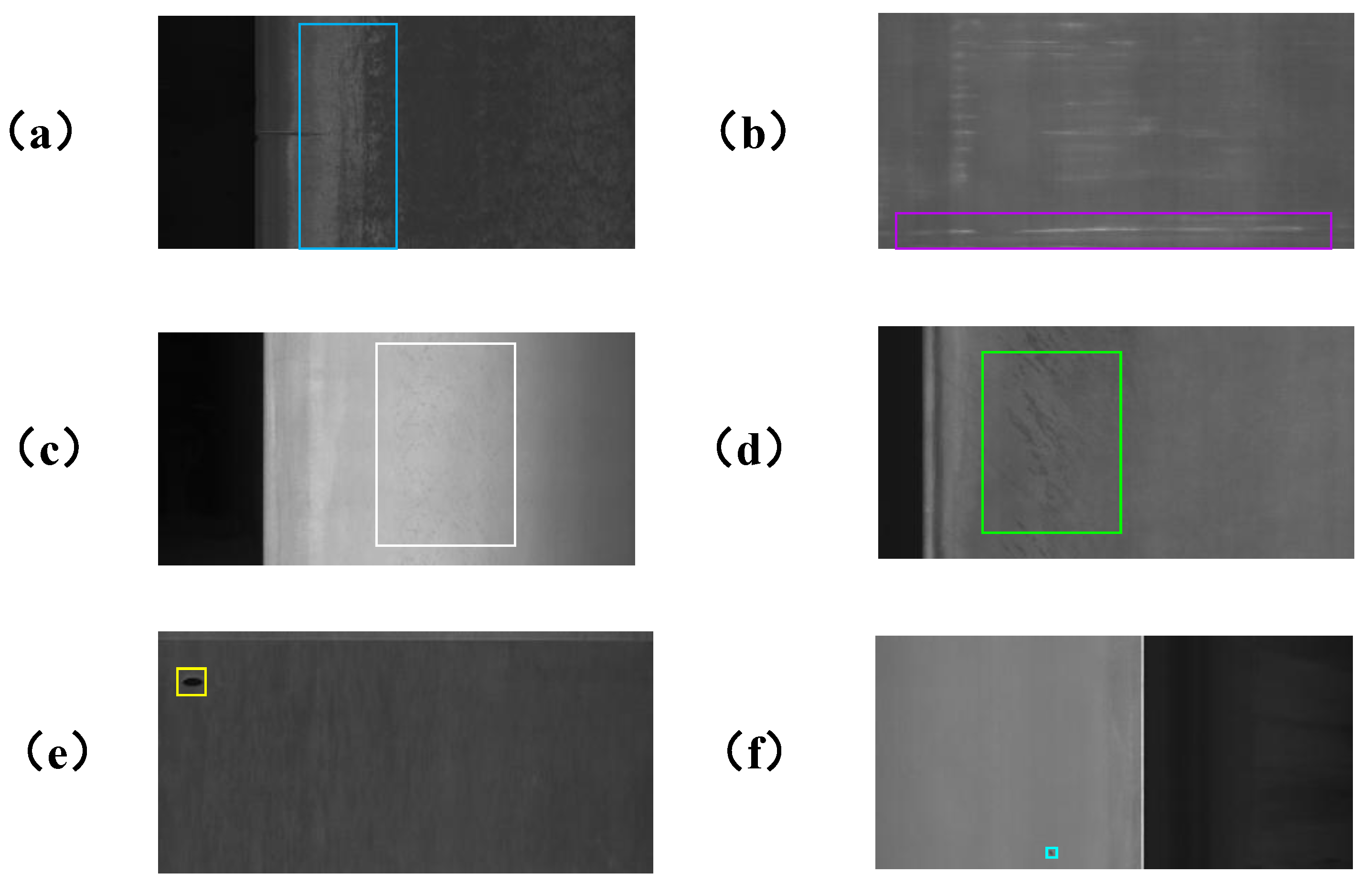
To verify the advantages of the RFCAConv module in detecting long-range spatial dependencies and low-contrast defects, we conducted comprehensive comparison experiments based on the baseline model. As shown in

Table 4. Performance comparison of attention modules in detecting long-range spatial dependency defects.

Module	Crease (Long-Range Defects1)		Waist Folding (Long-Range Defects2)
	mAP@0.5/%	mAP@0.5–0.95/%	mAP@0.5/%	mAP@0.5–0.95/%
YOLO11 (Baseline)	25.2	12.4	90.2	49.7
+SE [36]	31.2	15.8	91.3	50.2
+CBAM [37]	35.8	18.2	91.9	50.2
+RFCAConv	53.0	20.8	92.5	50.4

and

Table 5. Performance comparison of attention modules in detecting low-contrast defects.

Module	Silkspot (Low-Contrast Defects1)		Water Spot (Low-Contrast Defects2)
	mAP@0.5/%	mAP@0.5–0.95/%	mAP@0.5/%	mAP@0.5–0.95/%
YOLO11 (Baseline)	52.2	23.2	71.4	38.2
+SE [36]	55.8	24.1	72.8	39.1
+CBAM [37]	58.1	25.3	74.2	39.6
+RFCAConv	60.2	26.1	75.8	40.3

, for the two typical long-range spatial dependency defects (Crease and Waist folding), RFCAConv improved mAP@0.5 by 27.8% and 2.3% and mAP@50–95 by 8.4% and 0.7%. For the two typical low-contrast defects (Silkspot and Water spot), it enhanced mAP@0.5 by 8% and 4.4% and mAP@0.5–95 by 2.9% and 2.1%.

To achieve the best balance between receptive field expansion, edge information retention, and global feature capture, we explored various dilation rate combinations. The pixel utilization distribution for each combination is shown in Figure 8a–e. The r = [1,1,1] combination had slow receptive field expansion and focused on local information. The r = [1,2,3] combination’s receptive field grew with increasing dilation rates but payed less attention to edge details. The r = [2,1,2] combination balanced receptive field expansion and edge retention but had limited global feature capture. The r = [2,2,2] combination, with a common factor greater than 1, caused detail loss. Finally, the r = [1,3,5] combination rapidly expanded the receptive field and achieved the best balance between global features and edge information. We then verified the impact of dilated convolutions with different dilation rates on network predictions, with the results shown in

Table 6. Comparison of network performance with different dilation rates in dilated convolutions.

Dilation Rates	mAP@0.5/%	mAP@0.5–0.95/%	Precision	Recall
$r=[1,1,1]$	66.0	33.1	63.2	60.7
$r=[1,2,3]$	65.0	33.2	63.8	64.0
$r=[2,1,2]$	65.2	30.6	62.5	65.3
$r=[2,2,2]$	62.1	31.2	61.8	60.4
$\mathit{r}=[\mathbf{1},\mathbf{3},\mathbf{5}]$	65.3	33.2	64.0	65.7

. The r = [1,3,5] combination showed the best performance in mAP@0.5, mAP@0.5–0.95, Precision, and Recall.

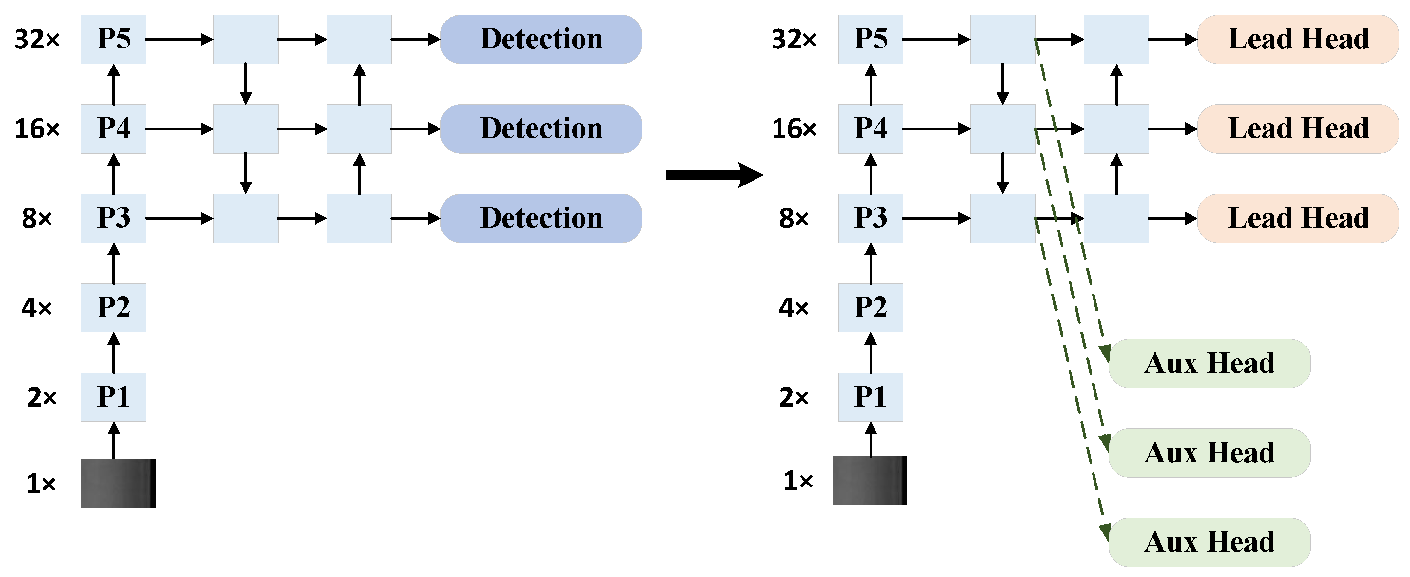
To validate the effectiveness of the Aux Head module for small-target defect detection, we performed multiple comparative experiments based on the baseline model, with detailed results presented in

Table 7. Performance comparison of different detection modules in detecting small defects.

Module	Punching (Small Defect1)		Inclusion (Small Defect2)
	mAP@0.5/%	mAP@0.5–0.95/%	mAP@0.5/%	mAP@0.5–0.95/%
YOLO11 (Baseline)	97.6	55.5	41.4	13.0
+SEAMHead [38]	96.8	54.2	40.1	12.3
+EfficientHead [39]	95.4	52.7	38.5	11.8
+PGI [40]	98.1	56.3	42.0	13.2
+Aux Head	98.7	57.5	43.8	13.8

. The experimental results demonstrated that for two representative small-target defect categories—Punching and Waist folding—the Aux Head module achieved optimal performance, showing improvements of 1.1% and 2.4% in mAP@0.5, along with enhancements of 2.0% and 0.8% in mAP@0.5–0.95 compared to the baseline, respectively.

To further validate the outstanding detection performance of FAD-Net, we conducted a comparative experiment on the GC10-DET dataset with mainstream detection algorithms: Faster-RCNN, DINO, Retinanet, RTMDET, RT-DETR, Swin-Transformer, and other YOLO series models. The experimental results are shown in

Table 8. Comparison of the performance of different algorithms on the GC10-DET dataset.

Model	mAP@0.5/%	mAP@0.5–0.95/%	FLOPs/G	Params/M	FPS
Faster-RCNN-r50 [8]	64.9	31.6	156.0	41.5	59.3
DINO-4scale [41]	66.5	33.3	205.0	47.6	25.2
Retinanet [42]	59.3	28.1	8.0	4.9	104.0
RTMDET-tiny [43]	66.6	33.3	170.1	37.9	64.7
RT-DETR-r50 [44]	62.0	30.4	125.7	4.2	76.9
Swin-Transformer-tiny [45]	63.0	29.9	77.6	29.7	135.3
YOLOv5n	62.6	31.9	7.1	2.5	395.5
YOLOv8n	63.2	30.4	8.1	3.0	354.8
YOLOv9t [15]	63.1	32.5	7.6	1.97	329.9
YOLOv10n [16]	60.5	30.2	6.5	2.3	305.3
YOLO11n (baseline)	63.3	32.7	6.3	2.5	402.0
FAD-Net (ours)	68.3	34.0	6.9	2.8	362.9

. FAD-Net achieved the best performance in terms of detection accuracy. Specifically, FAD-Net improved mAP@0.5 by 9% over RetinaNet and outperformed the high-precision two-stage detectors Faster-RCNN and DINO by 3.4% and 1.8%, respectively. When compared with other YOLO series algorithms, FAD-Net also achieved the highest detection accuracy. Notably, FAD-Net demonstrated superior computational efficiency while maintaining exceptional detection accuracy. Comparative analysis of floating-point operations (FLOPs) and parameter counts (Params) confirmed FAD-Net’s effective complexity control—a critical advantage for real-time structural health monitoring in urban infrastructure applications.

Figure 9 presents the model comparison results. YOLO-series algorithms, with their compact architectures and lower FLOPs/G, are more suitable for real-time inspection requirements of urban infrastructure steel structures, achieving superior balance between computational efficiency and detection speed. Comparative experiments revealed FAD-Net’s 5% mAP improvement over baseline models, demonstrating its distinct advantages.

To verify the generalization ability of the proposed framework for different types of defects in both structural components and road scenarios, cross-dataset evaluations were performed using the NEU dataset from Northeastern University and the RDD2022 road defect dataset, respectively. The NEU dataset comprises six common characteristic defect categories in structural components: rolled scale, patches, cracks, scratches, pitted surfaces, and inclusions, with 300 samples per class (1800 samples in total). The RDD2022 road defect dataset contains four common types of road surface defects: longitudinal cracks, transverse cracks, alligator cracks, and potholes, with a total of 173,767 samples. Both were split into training and validation sets at a ratio of 4:1. Generalization experiment results are shown in

Table 9. Generalizability experiment.

Dataset	Model	mAP@0.5/%	mAP@0.5–0.95/%	FLOPs/G	Params/M
NEU	YOLO11 (baseline)	76.5	42.7	6.3	2.5
	FAD-Net (ours)	79.0	44.6	6.9	2.8
RDD2022	YOLO11 (baseline)	56.4	28.9	6.3	2.5
	FAD-Net (ours)	59.2	30.5	6.9	2.8

. All models were trained and tested using the same hyperparameters as in Table 2.

Figure 10 presents a comparison of key metrics between the baseline model and our proposed FAD-Net model over 300 training epochs on the validation set. Figure 10a shows that FAD-Net significantly outperformed the baseline model in terms of mAP@0.5. Figure 10b further illustrates that under the mAP@0.5–0.95 evaluation standard, FAD-Net continued to perform excellently, with improvements observed at multiple IoU thresholds. Figure 10c,d show comparisons of Precision and Recall, where FAD-Net also significantly outperformed the baseline model, indicating its advantage in detection accuracy and recall rate. In conclusion, the FAD-Net model demonstrates higher accuracy and reliability in object detection tasks, validating its effectiveness.

Figure 11 presents the model’s prediction results, demonstrating the improvements of FAD-Net over the baseline model in terms of missed detection, false detection, and confidence level. Specifically, lower missed and false detection rates showed that the model’s feature extraction was more accurate and its ability to suppress background interference was stronger, highlighting the model’s robustness and generalization ability in complex scenarios. Higher confidence in detection boxes indicated a higher probability of the target being present, reflecting the model’s ability to capture more target details. The first set of images shows that FAD-Net detected defects missed by the baseline model, reducing the missed detection rate. The second set shows false detections from the baseline model, which FAD-Net successfully avoided. The third set further demonstrates that FAD-Net improved the detection accuracy of the baseline model.

5. Conclusions and Discussion

The proposed FAD-Net is an advanced deep learning framework targeting the detection of surface defects in steel materials used in urban infrastructure. It has three main innovations. First, the RFCAConv module, which uses a coordinated attention mechanism, can dynamically focus on key areas in the receptive field, thereby significantly enhancing the detection of long-distance and low-contrast defects. Second, the MSDFConv module, which uses dilated convolutions with varying dilation rates, effectively captures multi-scale information and addresses the problem of local detail loss in traditional spatial pyramid pooling. Third, the auxiliary head, which combines an optimized positive sample allocation strategy and a dynamic task-aligned assigner, performs feature fusion across multiple layers to improve the detection of small defects. The experimental results demonstrate the effectiveness of FAD-Net, with a 5% improvement in mAP@0.5 to 68.3% on the GC10-DET dataset. Cross-dataset validation on the NEU and RDD2022 datasets showed respective improvements of 2.5% and 2.8% in mAP@0.5 compared to the baseline model, indicating good generalization in defect detection.

Current algorithm optimization is mainly based on laboratory-environment validation and does not consider the computational constraints in industrial deployment. In the future, we will actively explore the deployment and application of the algorithm on edge devices and migrate it from the laboratory to real-world factory production processes to contribute to more reliable urban infrastructure inspection.