Ship Typhoon Avoidance Route Planning Method Under Uncertain Typhoon Forecasts

Abstract

Formulating effective typhoon avoidance routes is crucial for ensuring the safe navigation of ocean-going vessels. From a maritime safety perspective, this paper investigates ship route optimization under typhoon forecast uncertainty. Initially, the study calculates the probability of a ship encountering a typhoon based on the distribution of historical typhoon data within the radius of seven-level winds and the distance between the ship and the typhoon. Subsequently, the minimum safe distance is quantified, and a multi-objective ship route optimization model for typhoon avoidance is established. A three-dimensional multi-objective ant colony algorithm is designed to solve this model. Finally, a typhoon avoidance simulation experiment is conducted using Typhoon TAMRI and a classic route in the South China Sea as a case study. The experimental results demonstrate that under adverse conditions of uncertain typhoon forecasts, the proposed multi-objective typhoon avoidance route optimization model can effectively avoid high wind and wave areas of the typhoon while balancing and optimizing multiple navigation indicators. This model can serve as a reference for shipping companies in formulating typhoon avoidance strategies.

1. Introduction

The smooth and safe operation of ocean shipping is closely related to economic and social development, and meteorological navigation for ocean-going vessels is an important guarantee for safe ocean shipping. The optimal design of ocean shipping routes in typhoon environments is a key technical challenge in ensuring the safety of maritime transportation. As one of the most severe extreme meteorological disasters affecting ocean shipping, the strong winds, high waves, and poor sea conditions caused by typhoons can significantly reduce a ship’s maneuverability, increase navigation risks, and, in severe cases, lead to catastrophic consequences such as loss of control and capsizing [1,2,3].

Using route optimization theory to study the ship avoidance problem is the most effective method at present. The aim of the route optimization problem in the general sea state is to optimize the ship’s heading and speed to reduce the cost and emission during the voyage. Szlapczynska [4] considered constraints such as time, energy consumption, and safety and used the Pareto optimization method to obtain the optimal route planning scheme. Wang et al. [5] proposed a 3D Dijkstra optimization algorithm, which can generate the globally optimal ship routes and reduce fuel consumption by at least 5% in the analyzed scenario. Chen et al. [6] proposed a field theory-based multi-objective path optimization algorithm to construct a design scheme for Arctic routes with the objectives of safety, economy, and environmental friendliness. Ma et al. [7] proposed an improved cell-based approach to optimize ship routes and speeds in Emission Control Areas (ECAs) to minimize the total voyage cost. Zhang et al. [8] improved a multi-objective ant colony algorithm to optimize ship routes with travel time and navigational risk as the optimization objectives. Li [9] co-optimized the ship’s heading and speed by improving the A* algorithm to realize that the ship can safely avoid dangerous areas of wind and waves as well as reduce the ship’s fuel consumption. Zaccone et al. [10] proposed a new voyage optimization method based on three-dimensional dynamic planning, which takes into account the meteorological conditions, ship motion characteristics, and personnel comfort, and can solve the ship voyage with the lowest fuel consumption routes and speed profiles.

Among the existing studies, some studies (e.g., [4,5,8,9,10]) have effectively enhanced the safety performance of route planning models in dealing with general high wind and wave conditions by introducing additional wind and wave constraints. However, typhoons, as a special type of extreme meteorological phenomenon, are characterized by much more than general windy and wave conditions and exhibit higher danger and complexity. Specifically, the wind level of typhoons is usually up to 12 or even higher, while the general wind and waves are mostly between 8 and 10; in addition, typhoons have uncertainty in their paths and speed of movement, and usually last for a longer period of time, up to several days or even more than a week, and have a wide range of impacts, often covering hundreds to thousands of kilometers of sea area. In contrast, the general large wind and wave weather is mostly a localized emergent event with short duration, small spatial extent which is easy to predict, and other characteristics. Therefore, the traditional route optimization model based on wind and wave constraints has insufficient security when facing typhoon scenarios, and more complex and dynamic avoidance strategies are urgently needed to cope with it.

Although the existing literature has made significant progress in route optimization under regular sea conditions, its theoretical framework and methodological system make it difficult to effectively respond to the challenges of ship navigation in extreme weather conditions such as typhoons. Although ships typically adopt risk-averse navigation strategies, such as rerouting to avoid typhoon-affected areas, the traditional decision-making process relies mainly on the accumulated empirical knowledge of experienced captains and navigators [11,12]. As previous studies highlighted, this experience-based approach often results in sub-optimal typhoon avoidance route planning. This is evidenced by studies that have investigated optimal route strategies under typhoon conditions and heavy seas using simulation-based approaches and empirical studies using real ship data [13,14]. Some studies also use a method that is more commonly used in severe weather conditions, which is to set wind and wave constraints in the route optimization model to achieve the effect of avoiding typhoons by restricting the ship from entering the high wind and wave area [15,16,17,18]. In addition, Huang et al. [19] established a typhoon avoidance model based on the GRASP algorithm framework to optimize the structure of the candidate set of independent variables by minimizing the ratio of the time the ship spends within the dangerous radius of the typhoon to the total sailing time. Jin et al. [20] analyzed the avoidance behaviors of ships during Typhoons Soulik and Kangri using AIS data. By using the K-means clustering method, the avoidance patterns of ships in different time and space scales were revealed. Kwon et al. [21] proposed a statistical model to describe the storm avoidance behavior of merchant ships in the North Atlantic region. The model is based on wave return data for the year 2025 and analyzes the avoidance strategies of ships in the face of storms.

A major limitation of the existing typhoon avoidance route optimization research is the insufficient consideration of forecast uncertainties. In the actual navigation environment, there is significant uncertainty in the future trajectory of the typhoon and the dynamic changes in the scale of its wind circle. This key meteorological information mainly depends on the forecasts of meteorological forecasting departments, and the accuracy of the forecasts is affected by a variety of complex factors [22,23,24], making it difficult for ships to accurately obtain key parameters such as the radius of the future typhoon’s force seven wind circle and the center position when formulating typhoon avoidance strategies. As a result, it is impossible to accurately determine the hazardous areas to be avoided during navigation.

Based on the above practical needs, the objectives of this study are as follows: first, to quantify the uncertainty parameters of the radius of the level seven wind circle and the position of the center of the typhoon; second, to establish a prediction model for the probability of a ship encountering a typhoon; third, to construct a multi-objective route optimization model that comprehensively considers navigation risk, fuel consumption and sailing time; and finally, to design a multi-objective three-dimensional ant colony algorithm to solve the model.

The paper is structured as follows: Section 2 describes the overall framework and process design of the typhoon avoidance system; Section 3 focuses on analyzing the uncertainty characteristics of the typhoon center position and the seven-level wind circle, and establishes a probability calculation model for ships encountering typhoons; Section 4 systematically describes the design process of the typhoon avoidance route optimization method; Section 5 details the design and implementation of the model solving algorithm; and Section 6 verifies the effectiveness of the model through a practical case study.

2. Problem Description

This study is in two parts. The first part is the derivation of the calculation process for the probability of a ship encountering a typhoon. The framework is shown in Figure 1. Historical data on the track of typhoons in the northwest Pacific can be obtained from the Tropical Cyclone Data Centre of the China Meteorological Administration (CMA). Forecast information such as the typhoon’s center position and probability circle can be obtained from the Japan Meteorological Agency. Ships face difficulties in formulating typhoon avoidance plans due to uncertainties in the track and impact area. Ships must account for typhoon forecast uncertainties to adopt effective avoidance strategies and ensure navigational safety.

The second part of this paper is the design of an air route optimization method. The physical model is used to calculate the minimum safe distance by inputting typhoon forecast data obtained from the Japan Meteorological Agency (JMA). In addition, ship parameters and wind and wave forecasts obtained from the European Centre for Medium-Range Weather Forecasts (ECMWF) are used to calculate the speed and power corrections of the ship under actual sea conditions. The framework of the second part is shown in Figure 2. First, based on the physical model estimated by the radius of the seven-level wind circle, the minimum safe distance that the ship should maintain with the typhoon center in the future is dynamically defined, and the assessment mechanism and specific typhoon avoidance measures are elaborated. Then, considering the effect of actual sea conditions on the ship’s navigational performance, a speed and power correction model is introduced to more accurately reflect the ship’s navigational state in complex sea conditions. On this basis, a multi-objective optimization model for the ship’s typhoon avoidance route under typhoon forecast uncertainty scenarios is constructed. Finally, a three-dimensional multi-objective ant colony optimization algorithm is designed to solve the model taking into account its characteristics.

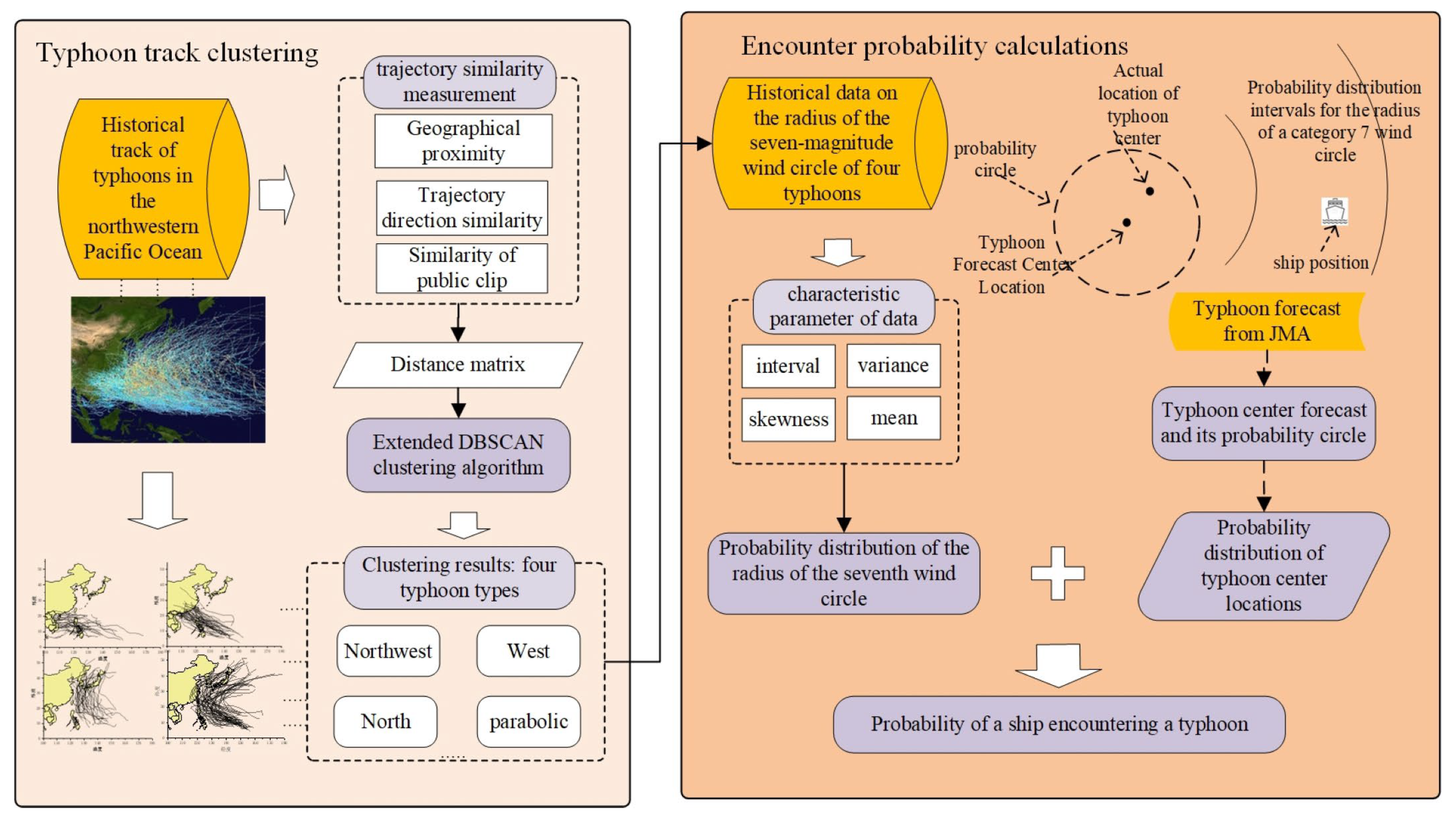
3. Probability Model for Ships Encountering Typhoons

This chapter describes a method for calculating the probability of a ship encountering a typhoon. Section 3.1 clusters historical typhoons. Section 3.2 derives the formula for calculating the Section 3.1.

3.1. Typhoon Track Clustering

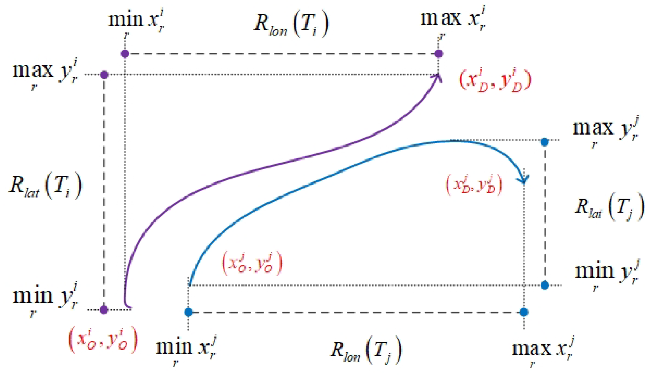
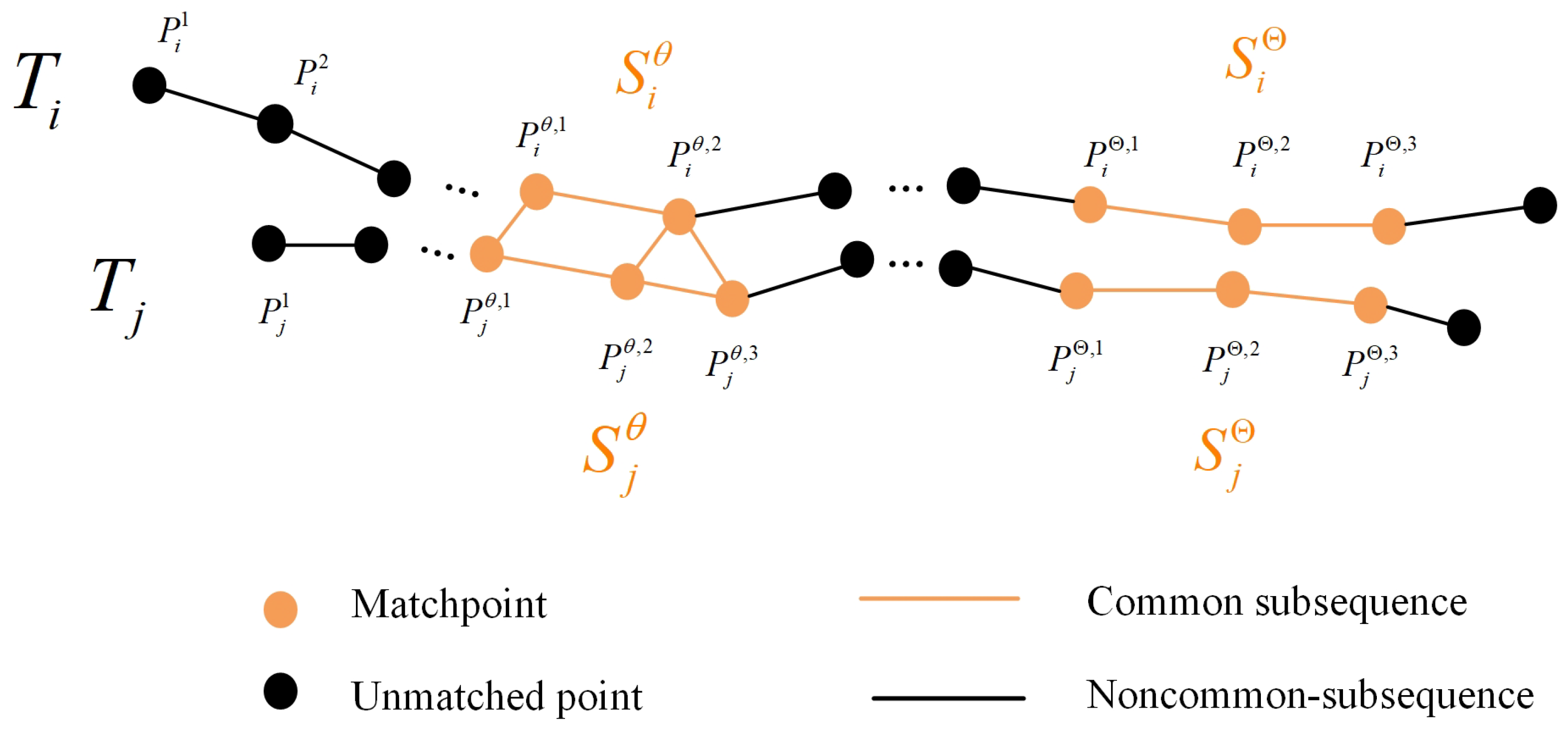
3.1.1. Trajectory Similarity Measurement

Trajectory similarity measurement [25,26] and calculation is a method used to compare the degree of similarity between two trajectories. A trajectory is considered to be a set of points, each of which has longitude and latitude coordinates and time information. In this paper, similarity is measured relative to the following features:

(1)

Geographical proximity

The similarity of the geographical areas of the two trajectories is represented by the degree of overlap of their longitude and latitude ranges. When the two trajectories are close to each other in space, their longitude and latitude ranges will overlap significantly; when the two trajectories are far apart in space, they will not overlap to a large extent in longitude and latitude. As shown in Figure 3, the longitude and latitude ranges of the two trajectories $T_i$ and $T_j$ are as follows:

$$R_{lon}\left(T_i\right)=\left[\underset{r}{\min } x_r^i,\underset{r}{\max } x_r^i\right]\begin{array}{cc}& r\in \left[1,2,..,n\right]\end{array}$$

(1)

The similarity between longitude and latitude intervals is calculated using the Jaccard formula for set similarity calculation, which is expressed as Equation (2):

$$J\left(A,B\right)={\displaystyle \frac{\left|A\cap B\right|}{\left|A\cup B\right|}}$$

(2)

The similarity between the two trajectories is defined as the average value of the Jaccard similarity in the longitude and latitude directions. Its value ranges from 0 to 1, and the formula is as follows:

$$GRS\left(T_i,T_j\right)={\displaystyle \frac{J\left(R_{lon}\left(T_i\right),R_{lon}\left(T_j\right)\right)+J\left(R_{lat}\left(T_i\right),R_{lat}\left(T_j\right)\right)}{2}}$$

(3)

(2)

Trajectory direction similarity

The similarity of the direction between any two trajectories can be expressed by the vector angle between the start and endpoint vectors of the trajectories. The coordinates of the start and endpoints form the OD vector, as shown in Figure 3. The OD vectors of $T_i$ and $T_j$ are expressed as $\underset{\left[x_O^i,y_O^i\right]\left[x_D^i,y_D^i\right]}{\to }$ and $\underset{\left[x_O^j,y_O^j\right]\left[x_D^j,y_D^j\right]}{\to }$, respectively, and the cosine of the included angle is given by the following:

$$\cos \left(T_i,T_j\right)={\displaystyle \frac{\overrightarrow{\left[x_O^i,y_O^i\right]\left[x_D^i,y_D^i\right]}\cdot \overrightarrow{\left[x_O^j,y_O^j\right]\left[x_D^j,y_D^j\right]}}{\Vert \overrightarrow{\left[x_O^i,y_O^i\right]\left[x_D^i,y_D^i\right]}\Vert \Vert \overrightarrow{\left[x_O^j,y_O^j\right]\left[x_D^j,y_D^j\right]}\Vert }}$$

(4)

Mapping the angle cosines of the OD vectors of trajectories $T_i$ and $T_j$ onto [0,1] yields the formula for the trajectory direction similarity DS:

$$DS\left(T_i,T_j\right)=1-{\displaystyle \frac{\arccos \left(\cos \left(T_i,T_j\right)\right)}{\pi }}$$

(5)

(3)

Trajectory public segment similarity

To compare the degree of similarity between the shapes of the two trajectories, this paper takes the similarity CCSS of the cumulative common sub-segments between the two trajectories as an indicator of the similarity of the trajectory’s common segment, as shown in Figure 4. The first step of calculating the CCSS is to determine the criterion of the matching point of the two trajectories, which first needs to be artificially set to a threshold value $\mathsf{\delta }$. The matching point will be when the distance between the path points on the two typhoon trajectories is smaller than $\mathsf{\delta }$. The CCSS is the first step in calculating the CCSS. All points on the trajectories that meet the requirements can be matched, so for any sampling point on one trajectory, there may be multiple sampling points on the other trajectory to match with, for example, the path point $p_i^{\theta ,2}$ on trajectory $T_i$ in Figure 4 can be matched with both sampling points $p_j^{\theta ,2}$ and $p_j^{\theta ,3}$ on the trajectory, but it does not affect the results of the calculation of CCSS.

Based on this matching principle, the common fragment formed by all the matching points on a trajectory is the set of common subsequences, and for a trajectory $T_i$ with Θ common subsequences, m is used to denote the θth common subsequence among them. The cumulative common subsequence lengths of trajectories $T_i$ and $T_j$ are denoted as follows:

$$l\left(S_{\chi }^{\theta }\right)={\displaystyle \sum _{m=1}^{m_{\chi }^{\theta }-1}{‖\left(p_{\chi }^{\theta ,m},p_{\chi }^{\theta ,m+1}\right)‖}_2}$$

(6)

where $l\left(S_x^{\theta }\right)$ is the length of the first common subsequence on the trajectory $T_{\chi }(\chi =i or j)$, $m_{\chi }^{\theta }$ is the number of path points contained in the $\theta$th common subsequence on the trajectory $T_{\chi }$, and ${‖·‖}_2$ is the Euclidean distance between any two points.

The lengths of the different trajectories are usually different, sometimes with large differences, so in order to minimize the effect of the length of the trajectories on the similarity of the trajectories, the CCSS is defined as the average of the cumulative common subsequence share corresponding to the two trajectories.

The CCSS for trajectories a and a containing Θ common subsequences is defined as follows:

$$CCSS\left(T_i,T_j\right)={\displaystyle \frac{1}{2}}{\displaystyle \frac{{\displaystyle {\sum }_{\chi }{\displaystyle {\sum }_{\theta =1}^{\mathrm{\Theta }}l\left(S_{\chi }^{\theta }\right)}}}{{\displaystyle {\sum }_{\chi }l\left(T_{\chi }\right)}}}$$

(7)

3.1.2. Trajectory Clustering Extension to the DBSCAN Clustering Algorithm

The traditional DBSCAN algorithm is mainly used for the clustering of points in space; the algorithm can identify the clusters formed by the points to be clustered in that space, but also to distinguish between noisy points, it is usually necessary to determine the two parameters, respectively, $eps$ and $Minsamples$, among which $eps$ is used to describe the neighborhood distance threshold of the samples, and $Minsamples$ is used to indicate the number of points that must satisfy the existence of the minimum number of points in the neighborhood when a point identifies as a core point [25,26]. The clustering algorithm used in this paper is an extended DBCSAN algorithm designed specifically for the scenario of trajectory clustering, the extended DBSCAN algorithm for trajectory clustering needs to expand the core neighborhood of a single distance parameter into a comprehensive neighborhood constructed from a variety of similarity metrics, capable of identifying the three types of similarity of trajectories in terms of features.

Therefore, three neighborhood thresholds ${eps}_g$, ${eps}_d$, and ${eps}_c$ are established here, corresponding to the three similarities GRS, DS, and CCSS mentioned in Section 3.1.1; for a certain trajectory, it needs to satisfy these three neighborhood ranges at the same time to be called the comprehensive neighborhood of the trajectory, which is calculated as follows:

$$D_g\left(T_i,T_j\right)=1-GRS\left(T_i,T_j\right)$$

(8)

$$D_d\left(T_i,T_j\right)=1-CS\left(T_i,T_j\right)$$

(9)

$$D_c\left(T_i,T_j\right)=1-CCSS\left(T_i,T_j\right)$$

(10)

Definition of DBSCAN and related concepts for expanding the core neighborhood:

(1)

The integrated domain $N_{{\epsilon }_g,{\epsilon }_c,{\epsilon }_d}\left(T_i\right)$ of the trajectory is defined as follows:

$$N_{{\epsilon }_g,{\epsilon }_c,{\epsilon }_d}\left(T_i\right)=\left\{D_g\left(T_i,T_j\right)\le {\epsilon }_g,D_d\left(T_i,T_j\right)\le {\epsilon }_d,D_c\left(T_i,T_j\right)\le {\epsilon }_c\right\}$$

(11)

(2)

On direct density reachability

The direct density reachability of trajectories $T_i$ and $T_j$ needs to satisfy the following two conditions: First, the trajectory $T_j$ is a trajectory that belongs to the range of the integrated neighborhood of the trajectory $T_i$ and $T_i$ is a core trajectory. The second is that the number of trajectories in the integrated neighborhood of trajectory $T_i$ is greater than $Minsamples$.

(3)

Density up to

If each trajectory $T_{n+1}$ in a sequence of trajectories $T_i,\dots ,T_n,T_{n+1},\dots ,T_j$ is directly density reachable with the previous trajectory $T_n$, then the $T_i$ and $T_j$ densities are reachable.

(4)

Density linked

Two trajectories $T_i$ and $T_j$ are said to be density-connected if they are both density-accessible.

The pseudo-code of the DBSCAN algorithm for trajectory clustering is shown in Algorithm 1:

Algorithm 1 DBSCAN algorithm for fusing multi-featured trajectory similarity
Input: Trajectory clustering set $\mathsf{\Phi }=\{T_1,T_2,T_3{,\dots ,T}_N\}$; Distance matrix ${\mathrm{D}}_g,{\mathrm{D}}_d,{\mathrm{D}}_c$;    Clustering parameter ${\mathsf{\epsilon }}_g,{\mathsf{\epsilon }}_d,{\mathsf{\epsilon }}_c,Minsamples$
Output: Cluster $\mathrm{C}=C_1,C_2,\dots ,C_n$, and, $C_n=\{T_1,T_2,T_3{,\dots ,T}_{\left|C_n\right|}\}$
1  set C$luster=0$         //Initialization
2  set all trajutories in $\mathsf{\Phi }$ as unvisited
3	if $T_i$ is not visited then
4		set $T_i$ as visited
5		get $N_{{\epsilon }_g,{\epsilon }_d,{\epsilon }_c}\left(T_i\right)$ using $D_g,D_d,D_c$
6			if $\left|N_{{\epsilon }_g,{\epsilon }_d,{\epsilon }_c}\left(T_i\right)\right|<Minsamples$ then
7			set $T_i$ as noise
8			else
9			C$luster=$ C$luster+1$     //Next cluster number
10			assign C$luster$ to all trajectories in $N_{{\epsilon }_g,{\epsilon }_d,{\epsilon }_c}\left(T_i\right)$
11			insert $N_{{\epsilon }_g,{\epsilon }_d,{\epsilon }_c}\left(T_i\right)-T_i$ into queue N
12			call $ExpandCluster \left(Cluster,i,N\right)$
13			return C
14	$\mathit{E}\mathit{x}\mathit{p}\mathit{a}\mathit{n}\mathit{d}\mathit{C}\mathit{l}\mathit{u}\mathit{s}\mathit{t}\mathit{e}\mathit{r}\left(Cluster,i,N\right)$
15	while N is not empty, do
16		remove $T_j$ from top of the N
17		get $N_{{\epsilon }_g,{\epsilon }_d,{\epsilon }_c}\left(T_j\right)$ using $D_g,D_d,D_c$
18		if $\left|N_{{\epsilon }_g,{\epsilon }_d,{\epsilon }_c}\left(T_j\right)\right|\ge Minsamples$ then
19		for $T_k$ in $N_{{\epsilon }_g,{\epsilon }_d,{\epsilon }_c}\left(T_j\right)$ do
20		if $T_k$ is visited or noise then
21		assign C$luster$ to $T_k$
22		if $T_k$ is not visited then
23		insert $T_k$ into N

3.1.3. Quality Assessment of Trajectory Clustering

In order to comprehensively evaluate the effectiveness of the extended DBSCAN algorithm proposed in this paper for typhoon track clustering, three widely used unsupervised clustering quality assessment metrics are introduced in this paper: the Silhouette Coefficient, the Davies–Bouldin Index, and the Calinski–Harabasz Index. The above indices measure the quality of clustering results in terms of dimensions such as inter-class separation, intra-class tightness, and clarity of cluster structure, respectively.

In this paper, the proposed method is compared with two classical clustering methods (K-means and TRACLUS) in a comparative experiment. The results show that the extended DBSCAN algorithm outperforms traditional methods across all three metrics, especially with better adaptability and differentiation ability when dealing with non-regular and complex shaped typhoon tracks.

3.1.4. Typhoon Cluster Results

In this paper, the extended DBSCAN algorithm is used to cluster historical typhoon tracks. The historical typhoon track data are obtained from the Tropical Cyclone Data Centre of the China Meteorological Administration (CMA). Since the typhoon tracks during the 2014–2022 vintage period retained more complete information (including wind circle data), the typhoon track data occurring during this period are selected for track clustering. The quality of clustering is assessed as shown in

Table 1. Comparison of clustering quality assessment.

Clustering Method	Silhouette ↑	DBI ↓	CH ↑
Expanded DBSCAN	0.672	0.395	531.7
K-means	0.441	0.739	370.4
TRACLUS	0.528	0.602	413.9

Note: ↑ means the higher the value the better, ↓ means the lower the value the better.

and the number of typhoons in each category is shown in

Table 2. Cluster results for the number of typhoons of various types.

Type of Typhoon Track	Number
Northwestern	58
Western	47
Parabolic	66
Northern	39
Noise track	11
Total quantity	221

, in which there are five types of tracks with obvious regularity characteristics, i.e., westward traveling, northwestward traveling, upward traveling to the north, and parabolic trajectories. The statistics of the wind circle radius data at level seven are shown in Figure 5.The interval parameters and data characteristics of the Class VII wind circle are shown in

Table A1. Value of the radius of the wind circle in Beaufort scale 7.

Typhoon Type	Interval (a, b)	NE	SE	SW	NW
Northwestern	a	43.19	32.39	26.99	26.99
	b	323.97	269.97	259.18	269.97
western	a	37.79	26.99	26.99	32.39
	b	242.98	215.98	194.38	296.98
Northern	a	23.32	23.32	21.59	26.23
	b	269.97	269.97	215.98	215.98
parabolic	a	32.39	43.19	26.99	26.99
	b	242.98	242.98	215.98	269.97

and

Table A2. Skewness $\lambda$, mean $\mu$, and variance $\sigma$ of the historical data for the radius of the seventh wind circle.

Typhoon Type	Value	NE	SE	SW	NW
Northwestern western	$\lambda$	0.68	0.53	0.53	0.36
	$\mu$	141.04	132.35	123.15	124.21
	$\sigma$	54.13	50.06	47.67	47.36
Northern	$\lambda$	00.01	0.37	0.17	0.11
	$\mu$	126.57	102.80	104.92	135.55
	$\sigma$	43.98	39.36	38.58	50.80
parabolic typhoon type	$\lambda$	0.54	0.57	1.02	0.72
	$\mu$	116.43	117.64	95.78	93.25
	$\sigma$	55.42	59.15	50.26	44.57
Northwestern	$\lambda$	−0.24	0.49	0.53	0.57
	$\mu$	128.48	132.17	109.44	114.67
	$\sigma$	48.89	52.52	49.09	56.33

, respectively.

3.2. Calculation of the Probability of a Ship Encountering a Typhoon

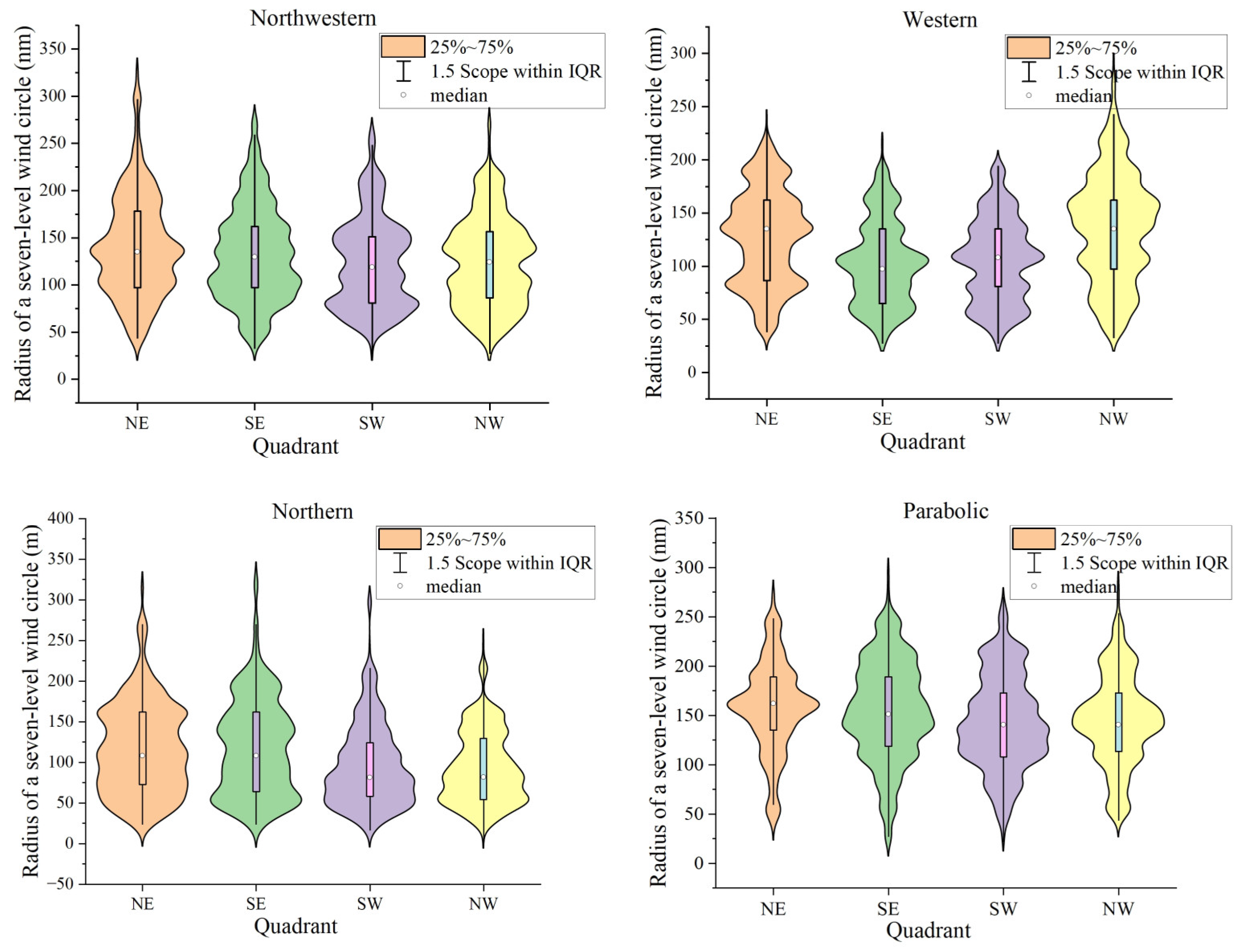
3.2.1. Probability Distribution of the Radius of the Seventh Wind Circle

According to the statistical results of the seven-level wind circle radius in Section 3.1.3, this article uses the skew distribution function to express the distribution of the radius of the seven-level wind circle. The values of skewness $\lambda$, mean $\mu$, variance $\mathsf{\sigma },$ and range of the radius of the typhoon seven-level wind circle $\left(a,b\right)$ for different categories are shown in Appendix A.

First, the probability density expressions for the skewed distributions are shown in Equations (12) and (13):

$$\psi (x)=2\varphi (x)\mathsf{\Phi }(\lambda x)$$

(12)

$$\mathsf{\Psi }(x)=2{\displaystyle {\int }_{-\infty }^x\varphi (t)\mathsf{\Phi }(t)dt}$$

(13)

Among them, $\varphi \left(x\right)$ and $\mathsf{\Phi }\left(x\right)$ are the probability density function and cumulative distribution function of the standard normal distribution, respectively.

Since the historical data of the radius of the seven-level wind circle falls within the range of the minimum and maximum data values, a truncation interval needs to be set for the skewed distribution function, which is denoted by (a, b). Therefore, the probability density and cumulative distribution expressions of the truncated skewed distribution are shown in Equations (14) and (15), respectively.

$$f_R\left(a,b;r\right)=\left\{\begin{array}{cc}0& r\le a\\ {\displaystyle \frac{\psi \left(r\right)}{\mathsf{\Psi }(b)-\mathsf{\Psi }(a)}}& a<r<b\\ 0& b\le r\end{array}\right.$$

(14)

$$F_R\left(a,b;r\right)=\left\{\begin{array}{cc}0& r\le a\\ {\displaystyle \frac{\mathsf{\Psi }(b)-\psi \left(r\right)}{\mathsf{\Psi }(b)-\mathsf{\Psi }(a)}}& a<r<b\\ 1& b\le r\end{array}\right.$$

(15)

3.2.2. Representation of Typhoon Center Location Probability

In typhoon track forecasting, the typhoon center position may appear at any position in the probability circle with the typhoon center forecast position as the center and the probability error as the radius, and the typhoon center forecast position is denoted as $\left(X_f,Y_f\right)$. In the absence of other known constraints, based on the maximum entropy principle [27], we assume that the typhoon center (X_c, Y_c) obeys a two-dimensional uniform distribution in the probability circle D, denoted as $\left(X_c,Y_c\right)\sim U_D$, and the radius of the probability circle is $E$. Its probability density function is as follows:

$$f_{X_c,Y_c}\left(x,y\right)=\left\{\begin{array}{cc}{\displaystyle \frac{1}{\pi E^2}}& \sqrt{\left(x-X_f\right)+\left(y-Y_f\right)}\le E\\ 0& \sqrt{\left(x-X_f\right)+\left(y-Y_f\right)}>E\end{array}\right.$$

(16)

3.2.3. Calculation of the Conditional Probability of a Ship Encountering a Force 7 Wind Circle

First, the position of the ship is denoted as $\left(X_s,Y_s\right)$ and the distance between the ship and the position of the typhoon center is denoted as F. There are the following:

$$\alpha =\sqrt{{\left(X_{\mathrm{c}}-X_{\mathrm{s}}\right)}^2+{\left(Y_c-X_s\right)}^2}$$

(17)

The typhoon’s seven-level wind circle obeys a skewed distribution in the interval (a, b), and the cumulative probability function is derived as shown in Equation (15), denoted a $F_R\left(a,b,r\right)$. Given that the center of the typhoon $\left(X_c,Y_c\right)$ is fixed, the probability of the ship encountering a wind circle of force 7 is as follows:

$$\begin{array}{l}P\left(\alpha \le R\left|X_c=x,Y_c=y\right.\right)=P\left(\sqrt{{\left(x-X_s\right)}^2+{\left(y-Y_s\right)}^2}\le R\right)\\ =F_R\left(\sqrt{{\left(x-X_s\right)}^2+{\left(y-Y_s\right)}^2}\right)\end{array}$$

(18)

By integrating the location $\left(X_c,Y_c\right)$ of the typhoon center within the probability circle D, the total probability $P_{encounter}$ of the ship encountering a wind circle of force 7 is obtained:

$$\begin{array}{c}{P}_{encounter}=P\left(\alpha \le R\right)\hfill \\ \begin{array}{c}\hspace{1em}={\displaystyle {\iint }_{\sqrt{{\left(x-X_s\right)}^2+{\left(y-Y_s\right)}^2}\le E}{F}_R\left(a,b;\sqrt{{\left(x-X_s\right)}^2+{\left(y-Y_s\right)}^2}\right)}\cdot f_{X_c,Y_c}\left(x,y\right)dxdy\hfill \end{array}\end{array}$$

(19)

Substituting the expression of $f_{X_c,Y_c}\left(x,y\right)$ into Equation (10) gives the following:

$$P_{encounter}={\displaystyle \frac{1}{\pi E^2}}{\displaystyle {\iint }_{\sqrt{{\left(x-X_f\right)}^2+{\left(y-Y_f\right)}^2}\le E}{F}_R\left(a,b;\sqrt{{\left(x-X_s\right)}^2+{\left(y-Y_s\right)}^2}\right)}dxdy$$

(20)

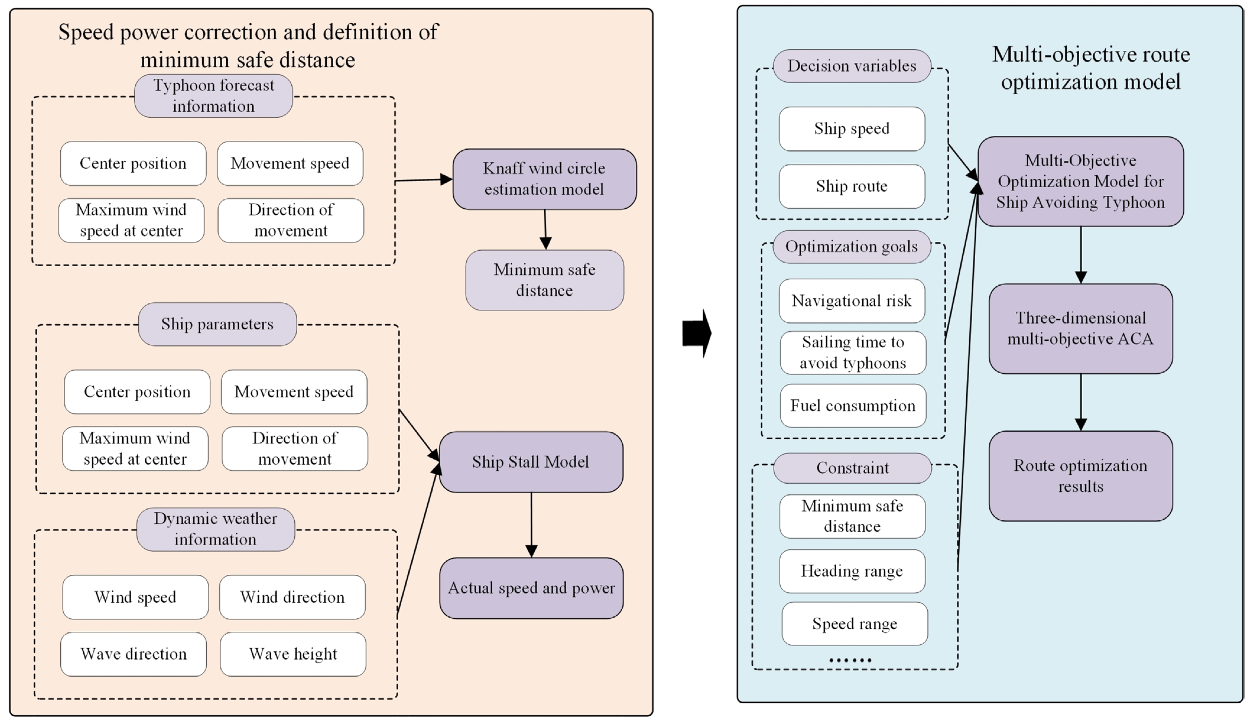
4. Optimization Methods and Models for Avoiding Platform Routes

This section describes the design of the method for optimizing the route to avoid the typhoon. Section 4.1 introduces a method for quantifying the minimum safe distance, and Section 4.2 introduces a method for determining whether to take action to avoid the typhoon. Section 4.3 establishes a multi-objective route optimization model for ships avoiding typhoons.

4.1. Quantification of Minimum Safety Distances

In the ship typhoon avoidance strategy, the purpose of defining the minimum safe distance is to provide a dynamic safety constraint for ship navigation to minimize the risk of ships encountering typhoons. The core idea is based on the Knaff physical model [28,29]. By inputting key forecast information such as the strength and movement speed of the typhoon and its latitude, the radius distribution of the typhoon’s wind circle at different times in the future is estimated in the four quadrants (NE, SE, SW, and NW), and this is used as the minimum safe distance that the ship needs to maintain between itself and the typhoon’s center at different times in the future and in different directions.

$$\mathrm{r}\left(\theta \right)={\mathrm{r}}_m\cdot {\left({\displaystyle \frac{34-a\cdot \cos \left(\theta -{\theta }_0\right)}{v_m-a}}\right)}^{-{\displaystyle \frac{1}{x}}}$$

(21)

$$\left\{\begin{array}{l}{\theta }_0=t_0+t_1\gamma +t_{2}c\\ a_c=a_0+a_{1}c+a_2{c}^2+a_3\gamma \\ x_c=x_0+x_1{v}_m+x_2\gamma \\ r_{mc}=m_0+m_1{v}_m+m_2\gamma \end{array}\right\}$$

(22)

In Equation (21), the radius of the wind circle $r$ is a function of the variable wind speed $v$ and the azimuth angle $\theta$. The radius of the seven-level wind circle is calculated by substituting 34 kn as the value of the wind speed $v$. This equation takes into account the asymmetry of the wind circle structure. In this paper, the values at azimuth angles of 45°, 135°, 225°, and 315° are calculated as the radius of the seven-level wind circle in the four quadrants of NE, SE, SW, and NW, respectively. In addition, the parameter $v_m$ in Equation (21) has one known parameter $v_m$ and four free parameters $r_m,x,a,\mathrm{a}\mathrm{n}\mathrm{d} {\theta }_0$. Among them, $v_m$ is the maximum wind speed near the center of the typhoon, $r_m$ is the radius of the maximum wind speed, $x$ is the dimensional parameter, $a$ is the asymmetry amplitude parameter, and ${\theta }_0$ is the directional angle of the typhoon moving direction rotated 90 degrees to the right. Equation (22) is an estimation equation for the four free parameters in Equation (21), where $\gamma$ and $c$ represent the latitude and typhoon movement speed, respectively, which can be obtained from typhoon forecast information. Knaff fitted the coefficients $t_0-t_2$, $a_0-a_3$, and $m_0-m_2$. The fitting results for the coefficients calculating the scale of typhoons in the northwestern Pacific region are shown in

Table 3. Values of parameters $t_0-t_2$, $a_0-a_3$, and $m_0-m_2$.

Parameter	Value	Parameter	Value
$t_0\left(°\right)$	−13.03	$x_0$	0.3151
$t_1$	0.8485	$x_1\left({kt}^{-1}\right)$	0.0038
$t_2\left(°{kt}^{-1}\right)$	1.0653	$x_2\left({degree}^{-1}\right)$	−0.0022
$a_0\left(kt\right)$	4.2980	$m_0\left(n mi\right)$	56.9200
$a_1$	−0.1574	$m_1\left(n mi {kt}^{-1}\right)$	−0.1541
$a_2\left({kt}^{-1}\right)$	0.0035	$m_2\left(n mi {degree}^{-1}\right)$	0.7372
$a_3\left({kt degree}^{-1}\right)$	0.1276	--	--

.

The results of the four-quadrant radius of the typhoon’s seven-level wind circle calculated using the above physical model are expressed as $r_{NE},{ r}_{SE},{ r}_{SW},\mathrm{a}\mathrm{n}\mathrm{d}{ r}_{NW}$. If the ship’s bearing to the typhoon at time t is expressed as ori, then the minimum safe distance ${L\left(ori\right)}_t$ to be maintained can be expressed as follows:

$$L{(ori)}_t=\left\{\begin{array}{cc}{r}_{NE}& ori=NE\\ r_{SE}& ori=SE\\ r_{SW}& ori=SW\\ r_{NW}& ori=NW\end{array}\right.$$

(23)

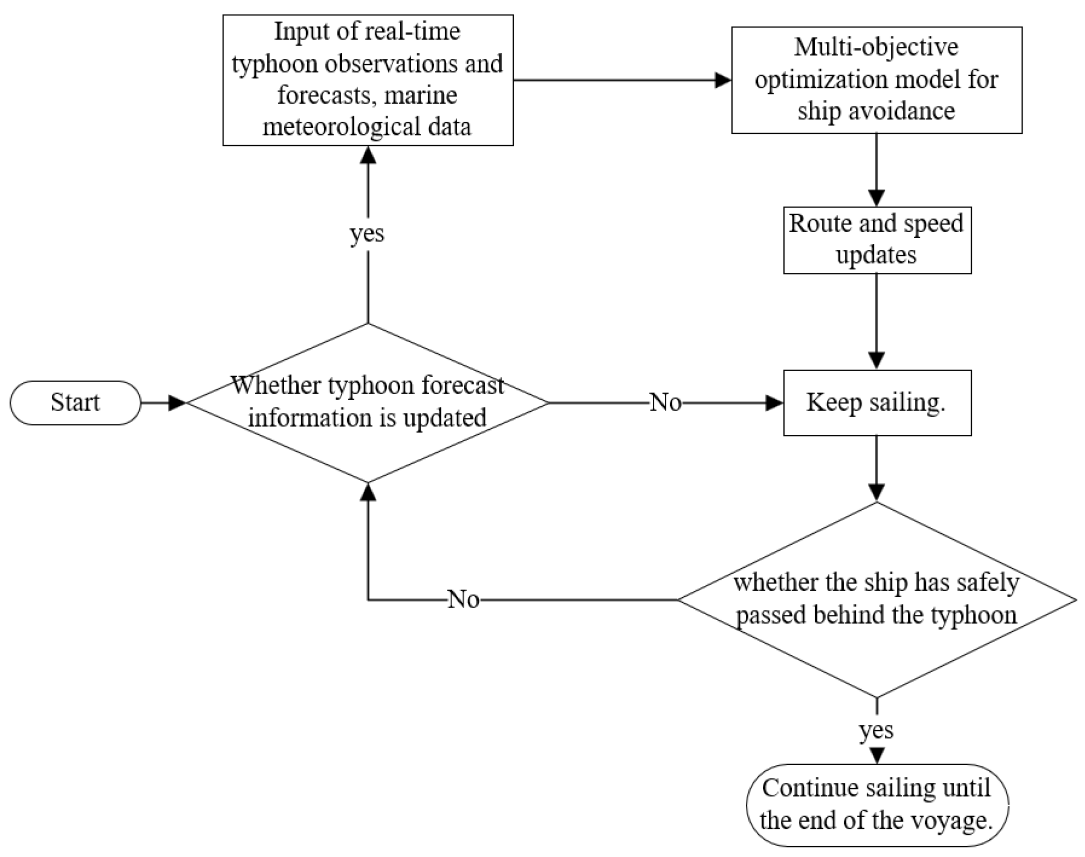
4.2. Judgment Method for Whether a Ship Should Take Evasive Action

When a ship is sailing in an area where a typhoon is passing through, it needs to determine whether it should maintain its current course and speed or change its sailing plan to avoid the typhoon. This article uses the estimated distance between the ship’s position at time t and the typhoon forecast center.

Therefore, the decision mechanism $A\left(t_0\right)$ for determining whether the ship should take action to avoid the typhoon at the current moment $t_0$ can be expressed as follows:

$$A\left(t_0\right)=\left\{\begin{array}{cc}1& d{\left(ship,tc\right)}_t\le L{\left(ori\right)}_t\\ 0& d{\left(ship,tc\right)}_t>L{\left(ori\right)}_t\end{array}\right.$$

(24)

Equation (24) states that when the distance between the estimated position of the ship and the typhoon forecast center is less than the minimum safe distance ${L\left(ori\right)}_t$, the value of $A\left(t_0\right)$ is taken as 1, indicating that typhoon avoidance operations should be carried out. Conversely, it indicates that typhoon avoidance operations are not necessary, and the ship can simply maintain its heading and speed.

4.3. Ship Route Optimization Model for Avoiding Typhoons

4.3.1. Model Parameter Definition

The specific symbols and meanings involved in the optimization model constructed in this paper are shown in

Table 4. Model notation and interpretation.

Symbol	Interpretation
$T_{\mathrm{t}\mathrm{o}\mathrm{t}\mathrm{a}\mathrm{l}}$	Total time of navigation avoiding typhoon/h
$Q_{\mathrm{T}\mathrm{o}\mathrm{t}\mathrm{a}\mathrm{l}}$	Total fuel consumption for avoiding the typhoon/ton
$R_{\mathrm{T}\mathrm{o}\mathrm{t}\mathrm{a}\mathrm{l}}$	General risk of navigation
$N$	Set of segments $N=\{1,\dots ,i,\dots ,N\}$
$v_w^i$	Drostatic speed of ship in the i-th leg/knots
$v_g^i$	Actual speed of ship in the ith leg/knots
$\theta$	Course of ship in the ith leg/degrees
$g$	Daily fuel consumption/ton
$l$	Leg length/nautical miles
$H$	Wave height/(m)
$V_{i,j}^a$	Wind speed/(m/s)
$t_0$	The moment the ship takes action to avoid the typhoon
${L\left(ori\right)}_t$	The minimum safe distance at all times is determined by the bearing of the Ship at $t$ moment to the center of the typhoon and the formula of the physical model of a wind circle of force 7.
$d_t$	Distance between the ship’s position and the typhoon center at $t$moment
$v_t$	The speed at $t$ moment is determined by the speed of the section of the waterway the ship is traveling through at $t$ moment.
$\left(x_t,y_t\right)$	The position of the ship at $t$ moment is determined by the position of the ship at $t$ moment at the point on segment ith.
$\mathsf{\Sigma }$	Areas with static obstacles such as islands and shorelines
$\mathsf{\lambda }$	Constant, the risk objective function multiplied by the probability of encountering a typhoon
$v_{\mathrm{m}\mathrm{i}\mathrm{n}}$/$v_{\mathrm{m}\mathrm{a}\mathrm{x}}$	The minimum/maximum speed limit/knots during the voyage of the ship is determined by the actual performance of the ship.
${\theta }_{\mathrm{m}\mathrm{i}\mathrm{n}}/{\theta }_{\mathrm{m}\mathrm{a}\mathrm{x}}$	Minimum speed limit during navigation/knots, determined by the actual situation of the route

.

4.3.2. Model Variable

In order to facilitate the calculation and comparison of optimization objectives, this study divides the route into multiple segments and discretizes the course and speed. Specifically, when a complete route consists of a series of waypoints, the independent variables of this paper’s model are the ship’s heading c at each waypoint and the speed v. As shown in Figure 6, the starting point of the segment ith, heading angle ${\theta }_i$, and the speed of the segment $v_w^i$ (taken as a scalar and a constant value) are included in the set of independent variables of the optimization model. After the optimization is completed, the optimized navigation route can be obtained by connecting all the waypoints and the endpoints of the route.

4.3.3. Optimization Objectives

(1)

Sailing Time for Avoiding Typhoon

For the ship avoiding a typhoon, navigation safety is the most important goal; in order to ensure navigation safety as much as possible, there is a need to minimize the time of the ship affected by the typhoon. The total time of avoiding a typhoon voyage $T_{total}$ is equal to the voyage distance of each section divided by the speed of navigation after considering the correction of the actual sea state.

$$T_{total}={\displaystyle \sum _{i=1}^N\frac{l_i\left({\theta }_i\right)}{v_g^i}}$$

(25)

(2)

Fuel consumption

Fuel is the most important component of the total cost of ship navigation, and this paper considers the speed as an optimization variable, while the ship’s variable speed is reflected in the design of platform avoidance routes that minimize fuel consumption. The formula for fuel consumption $Q_{total}$ is the multiplication of time, fuel consumption rate, and main engine power, so the power and fuel consumptions here are based on the values after power correction in considering the actual sea state.

$$Q_{total}={\displaystyle \sum _{i=0}^N{t}_i}\cdot {\displaystyle \frac{1}{24}}g\left(v_w^i\right)$$

(26)

(3)

Typhoon risk to ships

In a complete voyage, the ship’s position at different moments $\mathrm{t}$ is $\left({\mathrm{x}}_t,{\mathrm{y}}_t\right)$, and by calculating the probability of the ship encountering a typhoon at each moment (from the starting moment ${\mathrm{t}}_0$ of the typhoon avoidance to the end of the entire voyage at moment $\mathrm{T}$) one by one by t, the probability of the maximum value of the probability of the entire voyage is multiplied by a constant $\lambda$ as the risk measure of the ship encountering a typhoon.

$$Ris{k}_{total}=\lambda \cdot \underset{t\in \left(t_0,T\right)}{\max }\left\{P_{encounter}\left(x_t,y_t\right)\right\}$$

(27)

4.3.4. Multi-Objective Optimization Modeling of Ship Avoidance Routes

Based on the analysis of the ECA policy and the previous discussion on the optimization model, the multi-objective route optimization model for ships considering the ECA policy is constructed as follows:

$$\underset{x_t,y_t,v_t}{\min }f\left(\theta ,v\right)=[T_{total}(\theta ,v),Q_{total}(\theta ,v),Ris{k}_{total}]$$

(28)

The following constraints need to be satisfied:

$$v_{\min }<v_i<v_{\max }\begin{array}{cc},& \forall i\in I\end{array}$$

(29)

$${\theta }_{\min }<{\theta }_i<{\theta }_{\max }\begin{array}{cc},& \forall i\in I\end{array}$$

(30)

$$\left(x_{t+1},y_{t+1}\right)=\left(x_t,y_t\right)+v_t\cdot \mathrm{\Delta }t\cdot \left(\cos {\theta }_t,\sin {\theta }_t\right)$$

(31)

$$\left(x_t,y_t\right)\notin \Sigma$$

(32)

$$d_t>L{\left(ori\right)}_t$$

(33)

$$H_{i,j}<5\begin{array}{cc}& \forall i\in I,j\in J\end{array}$$

(34)

$$V_{i,j}^a<5\begin{array}{cc}& \forall i\in I,j\in J\end{array}$$

(35)

Constraint (29) and Constraint (30) are restrictions on the speed and course of the ship, i.e., the independent variable constraints of the ship, which are determined by the actual parameters of the ship and the actual route conditions. Constraint (31) is a constraint on the change in the ship’s position from time t to time t + 1. Constraint (32) restricts the geographical location of the ship during navigation, indicating that the ship must bypass static obstacle areas such as islands and land. Constraint (33) is a safety constraint on the ship’s navigation, limiting the minimum safe distance that the ship should maintain from the center of a typhoon. Constraints (34) and (35) restrict the wind and wave conditions in the area through which the ship passes, further ensuring the safety of the ship’s navigation.

When a ship is sailing at sea, its speed will decrease compared to that in calm water conditions. This phenomenon of speed reduction is called natural stall. The speed loss of the ship can be calculated as follows [29,30]:

$$\mathrm{\Delta }{v}_i=v_w^i-v_g^i={\displaystyle \frac{v_w^i{C}_{\beta }{C}_U{C}_{Form}}{100}}$$

(36)

In Formula (36), $∆v_i$ is the velocity loss of the $\mathrm{i}$th segment; $v_w^i$ is the static water velocity of the ith segment; $C_{\beta }$ is the directional attenuation coefficient, which is related to the ship’s encounter angle; $C_U$ is the velocity attenuation coefficient, which depends on the ship’s form factor and loading conditions and the Froude number $Fr$; and $C_{Form}$ is the ship’s form factor. See Reference [31] for the calculation of $C_{\beta }$, $C_U$, and $C_{Form}$.

This article uses an empirical formula to calculate the fuel consumption of the host machine.

$$g\left(v_w^i\right)=a{\left(v_w^i\right)}^3+a{\left(v_w^i\right)}^2+a{v}_w^i+d$$

(37)

In Formula (37), $g\left(v_w^i\right)$ is the daily fuel consumption of the host; a, b, c, and d are the fitting coefficients.

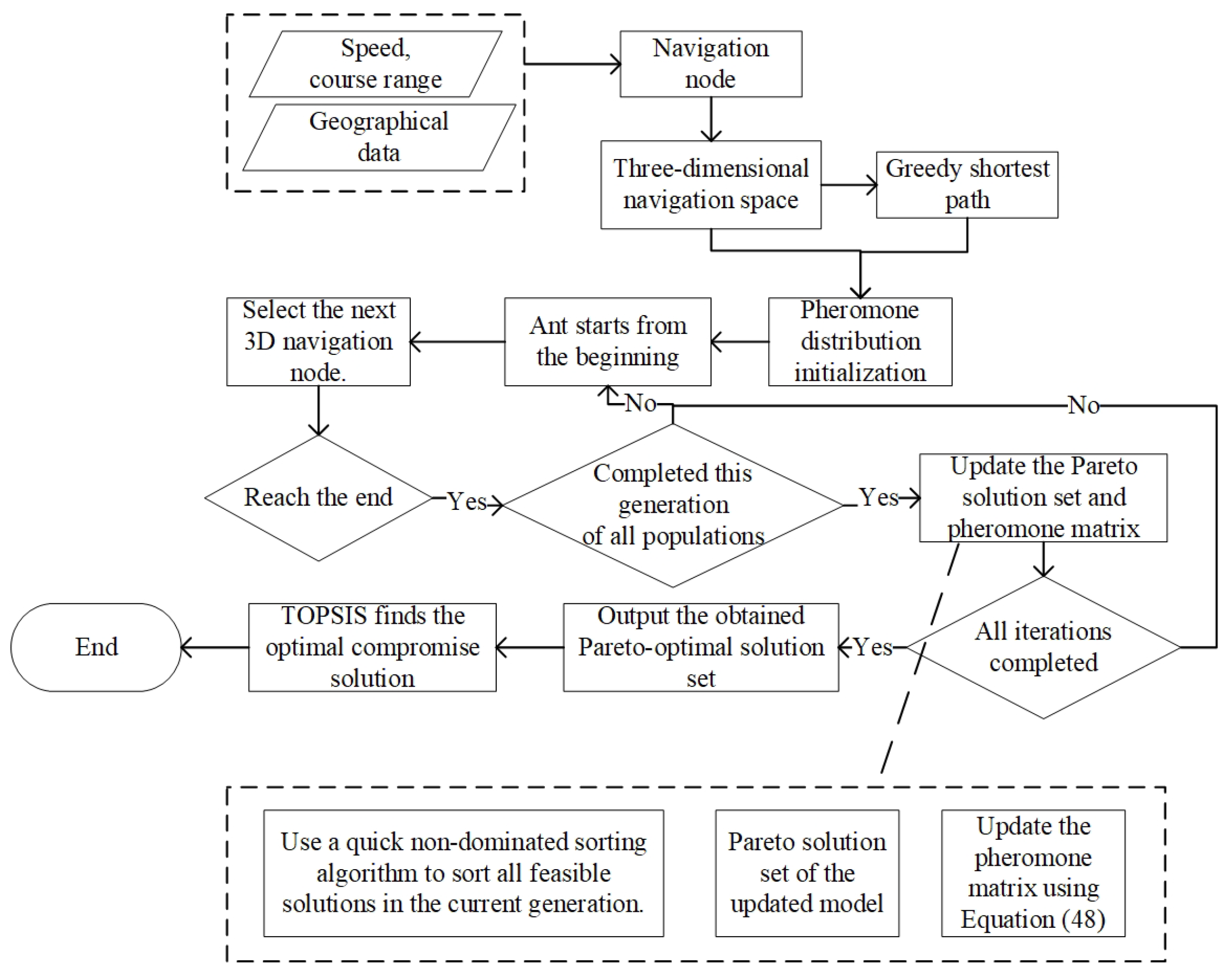
5. Solving Algorithm Design

This paper designs an improved three-dimensional ant colony optimization algorithm for avoiding obstacles. Section 5.1 introduces the principle of the basic ant colony algorithm and explains the process of using the basic ant colony algorithm for route optimization. Section 5.2 is the strategy for improving the search efficiency and convergence effect of the algorithm. Section 5.3 is the method of using the ant colony algorithm to solve multiple objectives. The flowchart of the multi-objective algorithm in this paper is shown in Figure 7.

5.1. Three-Dimensional Discretization of the Ship’s Navigation Space

In order to optimize the route, the two-dimensional geographic space from the starting point to the endpoint of the voyage needs to be discretized. On this basis, in order to also optimize the speed of the voyage, the speed range is discretized to construct a three-dimensional discretized voyage space. The specific process can be referred to in [31,32]. The three-dimensional discretized voyage space is shown in Figure 8, where the speed range is discretized into $v_{i,k\prime }^sϵ\left\{v_{min},v_{min}+\mathsf{\Delta }v,v_{min}+2\mathsf{\Delta }v,\dots ,v_{min}+k\mathsf{\Delta }v,{\dots ,v}_{max}\right\}$. In the figure, the state of the starting point A is $S\left(\mathrm{0,1},0\right)$, the starting point and ending point of the first path are the states $S\left(\mathrm{0,1},0\right)$ and $S\left(1,j,k\right)$, respectively, and the speed is expressed as $v_{1,k}$. i, j, and k represent the phase, state, and speed indices of the navigation, respectively; the starting point and ending point of the second path are the state points $S\left(1,j,k\right)$ and $S\left(2,j\prime ,k\prime \right)$, respectively. The speed is $v_{2,k}$ and so on until the end of the navigation.

5.2. Principles of Classical Ant Colony Algorithm

Ant colony algorithm (ACO) is a bionic class of intelligent algorithms first proposed by Italian scholars M Dorigo et al. in 1990 [33]. Used in this paper for solving the route optimization problem in three-dimensional navigation space, the basic steps of its search are as follows:

(1) The 3D navigation grid is constructed as in Figure 8, and the un-navigable path nodes due to regional constraints such as heading, speed, and island land are eliminated;

(2) The pheromone distribution of the nodes in the mesh system is initialized by using $\mathsf{\tau }$ to represent the pheromone structure of the entire 3D navigation mesh;

(3) The ant colony is allowed to start its search from the starting point and those potential nodes that can be reached in stage i + 1 are determined.

(4) The heuristic information ${\mathsf{\eta }}_{i+1,j,k}$ for each option in the potential nodes of stage i + 1 are calculated, where the heuristic information is the inverse of the estimated cost of that option to the endpoint, which can motivate the artificial ants to search for a route according to the set goal;

(5) The state transfer probability of each option is calculated using Equation (38) when an option is judged as not satisfying the safety constraint, i.e., the probability of that option is zero.

$$P_{\mathrm{i}+1,j,k}=\left\{\begin{array}{cc}{\displaystyle \frac{{\left({\tau }_{i+1,j,k}\right)}^{\alpha }{\left({\eta }_{i+1,j,k}\right)}^{\beta }}{{\displaystyle \sum {\left({\tau }_{i+1,j,k}\right)}^{\alpha }{\left({\eta }_{i+1,j,k}\right)}^{\beta }}}}& W\notin \mathrm{\Omega }\left(t\right)\\ 0& W\in \mathrm{\Omega }\left(t\right)\end{array}\right.$$

(38)

where ${\mathsf{\tau }}_{i+1,j,k}$ and ${\mathsf{\eta }}_{i+1,j,k}$ are the pheromone concentration and the amount of heuristic information of the node $\mathrm{i},\mathrm{j},\mathrm{k},$ and $\mathsf{\alpha }$, $\mathsf{\beta }$ are the pheromone concentration and the relevant importance level of the heuristic information, respectively. $\mathrm{W}\mathrm{e}\mathrm{d}\mathrm{e}\mathrm{n}\mathrm{o}\mathrm{t}\mathrm{e}$ the geographic location through which the ant chooses the option, which needs to be avoided to violate the safe distance constraint.

(6) Based on the calculated probability matrix, the next arrival node is selected by roulette rules, including geographic location and speed, until the target point is reached, forming a feasible trajectory;

(7) The objective function of the feasible routes for each ant that can reach the destination is calculated and the optimal route is memorized;

(8) The pheromone distribution is updated according to the nodes of the optimal route using Equations (39) and (40).

$${\tau }_{i,j,k}\left(t+1\right)=\left(1-\rho \right){\tau }_{i,j,k}\left(t\right)+\mathrm{\Delta }{\tau }_{i,j,k}$$

(39)

$$\mathrm{\Delta }{\tau }_{i,j,k}={\sum }_{m=1}^M\mathrm{\Delta }{\tau }_{i,j,k}^m$$

(40)

$$\mathrm{\Delta }{\tau }_{i,j,k}^{\mathrm{m}}\left(t\right)=\left\{\begin{array}{cc}{\displaystyle \frac{Q}{f\left(H_{\mathrm{m}}\right)}}& The ant passes through the path H_{\mathrm{m}}\\ 0& \mathrm{otherwise}\end{array}\right.$$

(41)

where $\mathsf{\rho }$ is the pheromone evaporation coefficient, $\mathsf{\Delta }{\tau }_{i,j,k}$ is the pheromone increase value, $\mathrm{Q}$ is the pheromone enhancement coefficient, and $f\left(H_m\right)$ is the surrogate value of the path traveled by this ant.

(9) The above steps are looped until the maximum number of iterations is reached.

This paper needs to solve the multi-objective platform avoidance route optimization problem at the same time, in order to improve the search efficiency, so to apply the ant colony algorithm in the model solution before making a series of targeted modifications to the algorithm in order to make it can be more efficient and accurate to obtain the optimal solution of the multi-objective platform avoidance route optimization model.

5.3. Three-Dimensional Discretization of the Ship’s Navigation Space

(1)

Greedy algorithm initializes pheromone distribution

Considering that the complexity of using the 3D ACO algorithm to solve the platform avoidance route optimization model is higher than that of the 2D ACO algorithm if the traditional ACO algorithm is used to directly initialize the pheromone matrix with a fixed value, the algorithm will need to wait for a longer iteration time before it can converge; therefore, this paper uses the greedy algorithm to initialize the pheromone matrix [34], and the specific process is as follows: starting from the sailing start point, each time we select the state point of the next section with the closest distance to the current stage node and the largest sailing speed in that stage as the next target section, and the target point access sequence is constructed according to this logic is used until all the sailing stages are traversed and the endpoint is reached, and then this path is used as the initial solution of the ACO algorithm for updating the pheromone structure so as to improve the convergence speed and the solving accuracy of the algorithm.

(2)

Elite Strategy

The updating of the pheromone is the core step in the formation of a positive feedback mechanism [35], and the basic idea of using the elite strategy to improve the way of updating the pheromone is as follows: at the end of each cycle, additional pheromone enhancement is given to the optimal solution found, the purpose of which is to make the optimal solution found up to the current position more attractive to the ants in the next time, and the pheromone is updated according to the following equation:

$${\tau }_{i,j,k}\left(t+1\right)=\left(1-\rho \right){\tau }_{i,j,k}\left(t\right)+\mathrm{\Delta }{\tau }_{i,j,k}+\mathrm{\Delta }{\tau }_{i,j,k}^{\ast }$$

(42)

where $∆{\tau }_{i,j,k}$ is the pheromone concentration released by all the ant colonies in that generation, which is calculated as shown in Equations (39) and (40); in addition to that, $∆{\tau }_{i,j,k}^{*}$ is the additional pheromone concentration enhancement given to the optimal solution, which is calculated as follows:

$$\mathrm{\Delta }{\tau }_{i,j,k}^{\ast }=\left\{\begin{array}{cc}\sigma {\displaystyle \frac{Q_1}{f\left(H*\right)}}& H* \mathrm{is} \mathrm{the} \mathrm{optimal} \mathrm{path}\\ 0& \mathrm{otherwise}\end{array}\right.$$

(43)

In Equation (43), which calculates $∆{\tau }_{i,j,k}^{*}$, $\sigma$ denotes the number of elite ants set, and $f\left(H^{*}\right)$ denotes the surrogate value of the optimal solution found.

5.4. Multi-Objective Ant Colony Algorithm Search Strategy

(1)

Comparison of feasible solutions based on fast nondominated sorting algorithms

The fast nondominated algorithm is an algorithm proposed by Deb et al. to quickly determine the order of merit of each feasible solution in a population. In the algorithm of this paper, the population is divided into several layers according to the dominance relationship: the first layer is the set of nondominated individuals selected from the population $F_1$; the second layer is the set of nondominated individuals obtained by removing the first layer $F_2$; the third layer is the set of nondominated individuals obtained by removing the first two layers $F_3$......, and so on. Subsequently, when performing the selection operation in the genetic operator, the first layer is considered $F_1$, then $F_2$, ......, and so on until the size requirement of the new population is satisfied.

Among other things, the definition of a non-dominant relationship is as follows:

The two feasible solutions of the multi-objective optimization problem are described as follows:

$$x_1=\left\{x_1^1,x_1^2,\dots ,x_1^m\right\}=F\left(x_1\right)=\left\{u_1^1,u_1^2,\dots ,u_1^m\right\}$$

(44)

$$x_2=\left\{x_2^1,x_2^2,\dots ,x_2^m\right\}=F\left(x_2\right)=\left\{u_2^1,u_2^2,\dots ,u_2^m\right\}$$

(45)

An individual $x_1$ is said to dominate $x_2\left(x_1\prec x_2\right)$ if the targets $F\left(x_1\right)$ and $F\left(x_2\right)$ fulfill the following conditions:

$$F\left(x_1\right)\prec F\left(x_2\right)\Rightarrow x_1\prec x_2$$

(46)

$$F\left(x_1\right)\prec F\left(x_2\right)iff\left[\exists i\in \left[1,2,\dots ,n\right],u_1^i\le u_2^i\right]\cap \left[\forall i\in \left[1,2,\dots ,n\right],u_1^i\le u_2^i\right]$$

(47)

In this case, the individual $x_1$ is the non-dominant individual.

In order to better obtain the Pareto solution set of the model, this paper uses the fast nondominated sorting algorithm in NSGA-II to sort the feasible solutions generated in each iteration, which serves as the basis for updating the routing pheromone in the subsequent steps and selects the solution whose sort is 1 to compare with the previous Pareto-optimal solution so as to update the Pareto-optimal solution set of the model.

(2)

Pheromone update based on nondominated ranking weights

When updating the pheromone, all the feasible solutions obtained in the current iteration will be used for updating, but the contribution of each feasible section to the amount of updating depends on the nondominated ranking weight of that solution, with the more highly ranked solution having a greater impact on the pheromone matrix. Let $Q_s$ be the pheromone constant of the $s$th sub-objective to limit the pheromone update rate, $\rho$ be the pheromone volatilization factor, $S_t$ be the set of feasible solutions for all the individuals in the$t$th iteration, ${Rank}_t^i$ be the ranking value of the individual $i$ solution after fast nondominated sorting of all the feasible solutions in $S_t$, $W_{rank}$ be the weight of the sorting value on the fitness, $O_t^i$ be the value of the $k$ th objective function for the individual $i$ solution, and ${\tau }_k^{t-1}$ be the pheromone matrix corresponding to the$k$th objective function after the last update, and be the pheromone matrix of the individual solution after the last update. Matrix $X_i^t$ is the 01 data structure of the path contained in the solution of individual $i$, the size of the data structure is the same as that of the pheromone data structure, and the value of the element is 1 means that the individual has passed through the path, otherwise, it is 0. Based on the definition of the above variables, the pheromone structure of the multi-objective ACO algorithm is updated as shown in Equation (48):

$${\tau }_k^t={\tau }_k^{t-1}\left(1-\rho \right)+{\displaystyle \sum _{n\in S_t}\frac{Q_k}{O_k^i\cdot Ran{k}_t^{i^{Wrank}}}}\cdot X_i^t$$

(48)

(3)

TOPSIS for compromise optimal solution

In a multi-objective optimization model, the problem of finding a compromise solution from a set of Pareto solutions can be regarded as a multi-attribute decision problem. In this paper, we need to find the compromise optimal solution in two steps, and the TOPSIS-based program decision process for this model is as follows:

Objective function homogenization: Keeps the objective function in the same trend. In the model of this paper, sailing time, total sailing fuel consumption, and sailing risk are all negative indicators (the smaller the better), so this step can be skipped:

1.

Raw matrix normalization:

$$C_{Total}\left(k\right)={\displaystyle \frac{C_{Total}\left(k\right)}{\sqrt{{\displaystyle \sum _{k=1}^w{\left(C_{Total}\left(k\right)\right)}^2}}}}$$

(49)

$$E_{Total}\left(k\right)={\displaystyle \frac{E_{Total}\left(k\right)}{\sqrt{{\displaystyle \sum _{k=1}^w{\left(E_{Total}\left(k\right)\right)}^2}}}}$$

(50)

where $k$ is the $k$th solution in the set of Pareto-optimal solutions and $w$ is the total number of individuals in the Pareto frontier.

2.

Obtain the solution vector after the virtual solution normalization:

$$“\mathrm{Virtual} \mathrm{Optimal} \mathrm{Solution}” \mathrm{for}: S^{+}=\min \left(C{\prime }_{Total},E{\prime }_{Total}\right)=\left[C{\prime }_{Total+},E{\prime }_{Total+}\right]$$

(51)

$$“\mathrm{Virtual} \mathrm{worst} \mathrm{solution}” \mathrm{for}: S^{-}=\max \left(C{\prime }_{Total},E{\prime }_{Total}\right)=\left[C{\prime }_{Total-},E{\prime }_{Total-}\right]$$

(52)

3.

Calculate the distance between the distance virtual solutions separately:

$$L{\left(k\right)}^{+}=\sqrt{{\left(C{\prime }_{Total}\left(k\right)-C{\prime }_{Total+}\right)}^2+{\left(E{\prime }_{Total}\left(k\right)-E{\prime }_{Total+}\right)}^2}$$

(53)

$$L{\left(k\right)}^{-}=\sqrt{{\left(C{\prime }_{Total}\left(k\right)-C{\prime }_{Total-}\right)}^2+{\left(E{\prime }_{Total}\left(k\right)-E{\prime }_{Total-}\right)}^2}$$

(54)

4.

Calculate the distance between the distance virtual solutions separately:

$$M\left(k\right)={\displaystyle \frac{L{\left(k\right)}^{-}}{L{\left(k\right)}^{+}+L{\left(k\right)}^{-}}}$$

(55)

Ultimately, the final solution is determined by referring to the $M\left(k\right)$ size ordering results. The purpose of selecting the optimal solution from the Pareto frontier can, thus, be realized. The resulting multi-objective optimization scheme for the ship can well achieve the compromise minimum.

6. Case Study

6.1. Background of the Example

6.1.1. Parameter Selection for Simulation Experiments

The ship parameters used in the experimental simulation of this paper are shown in Table 4.

Table 5. Selection of ship parameters for simulation experiments.

Vessel Parameters	Parameter Value
Overall length of vessel/(m)	332.95
Width of vessel/(m)	60
Length of ship’s waterline/(m)	332.6
Length between ship drogue lines/(m)	326.6
squareness factor	0.8026
Ship’s auxiliary engine power/(kW)	1440
Ship design speed/(knots)	14.1

lists the parameter selection of the simulation experimental algorithm, For the three objective functions, the ACO algorithm involves the updating process of the three pheromone matrices, so part of the parameters will be represented by a vector of length 3.

The main parameters of the proposed multi-objective 3D ACO algorithm include pheromone importance level $\mathsf{\alpha }$, heuristic information-related importance level $\mathsf{\beta }$, pheromone evaporation coefficient $\mathsf{\rho }$, pheromone enhancement coefficient $Q$, pheromone extra enhancement coefficient $Q_1$.

In order to obtain the best possible performance of the algorithm, this paper determines the parameters of the algorithm by using the Orthogonal Experimental Design (OED) method. OED detects some of the possible combinations between the factors instead of testing all of the combinations, which effectively reduces the number of trials and finds the optimal estimation of the factors during the execution. First, the values to be selected for each parameter are set: $\mathsf{\alpha }\in \left\{\mathrm{0.5,1},2\right\}$, $\mathsf{\beta }\in \left\{\mathrm{1,3},\mathrm{5,7},9\right\}$, $\mathsf{\rho }\in \left\{\mathrm{0.1,0.3,0.5,0.7,0.9}\right\}$, and $\mathrm{Q}\left(1\right)=\mathrm{Q}\left(2\right)=\mathrm{Q}\left(3\right)=Q_1\left(1\right)=Q_1\left(2\right)=Q_1\left(3\right)\in \left\{\mathrm{200,300,400,500,600}\right\}$. All the possible parameter combinations require $9^3=59049$ simulated experiments and the number of orthogonal designs is $L_{37}\left(9^5\right)$; therefore, only 37 experiments are included, which are selected to find the optimal parameter combinations as shown in

Table 6. Selection of basic parameters for simulation experiments.

Basic Parameters	Parameter Value
Number of iterations	50
Number of ants	30
Pheromone importance factor	(1, 1, 1)
Heuristic factor importance coefficients	(7, 7, 5)
Pheromone evaporation factor	(0.3, 0.3, 0.3)
Information literacy enhancement factor	(500, 300, 200)
Business Strategy Pheromone Additional Enhancement Factor	(600, 300, 200)
Number of elite ants	1

.

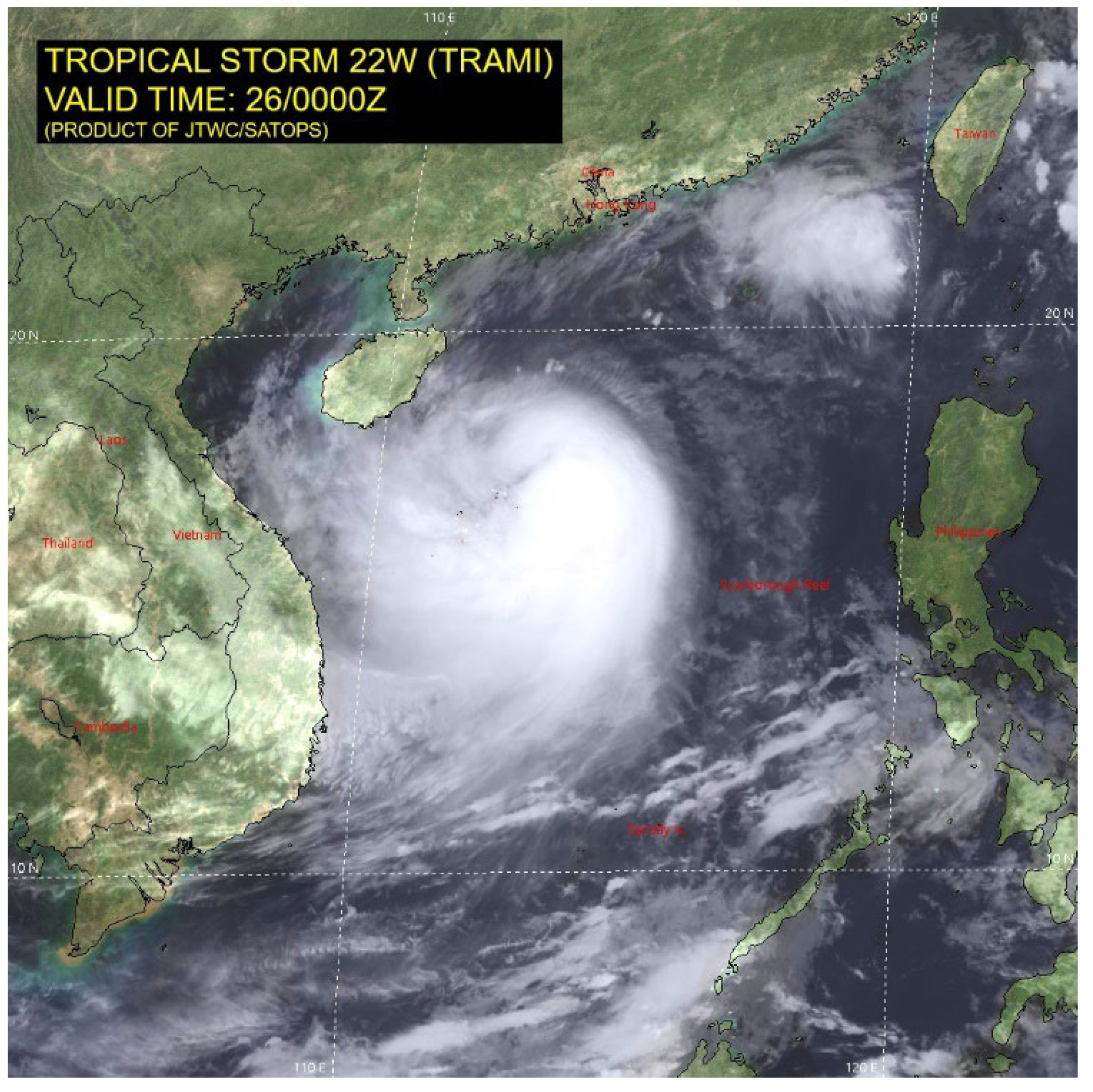
6.1.2. Typhoon Forecasting and Meteorological Data Acquisition

Typhoon TRAMI was named in the early morning hours of 22 October 2024 in the eastern part of the Philippines. Since then, it gradually developed and strengthened, and was upgraded to strong tropical storm level by the Central Weather Bureau (CWB) in the afternoon of 23 October, and made landfall in the province of Isabela, Philippines, in the early morning of the next day at the level of a strong tropical storm. Later, it entered the South China Sea and continued to develop and strengthen, and was upgraded to typhoon-level by the Central Weather Bureau on the morning of 26 October. It gradually weakened and made landfall on the coast near the border between Da Nang and Hue, Vietnam, on the morning of 27 October at tropical storm level. Figure 9 shows the satellite cloud map of Typhoon TRAMI.

The track of Typhoon TRAMI was generally westward, and this paper adopts the route from Singapore to Zhoushan Port as the planned route for the simulation case experiment 1, sailing at the design speed of the ship, departing at 07:00 on 22 October 2024 according to the observation and forecast information of Typhoon TRAMI, using the identification method of the timing of avoidance actions introduced in Section 4.2, and maintaining the identification of navigation risks during the voyage at 15:00 on the 23rd, the geographic location of the center of the typhoon was 16.14 N, 123.72 E.

The JMA’s typhoon forecast product releases real-time observations and real-time forecast data every 3 or 6 h, and the observations and forecast data released in each release, including geographic coordinates, the probability error radius of the typhoon center, i.e., the range of the probability circle; in addition, it also includes the central pressure value of the typhoon, the direction of the typhoon’s movement, and the speed of its movement. As shown in

Table 7. Observations and forecast information of Typhoon TRAMI at the starting point of avoidance of stations.

Time/h	Geographical Coordinates/N,E	Probability Circle Radius/nm	Center Pressure/hPa	Direction of Travel	Movement Speed/kn
0	16.1 N, 123.7 E	0	985	northwest	12
12	17.4 N, 121.6 E	40	985	northwest	10
24	16.4 N, 120.2 E	57	990	southwest	8
48	17.4 N,117.1 E	100	980	northwest	8
72	17.4 N, 113.1 E	120	975	west	10
96	17.2 N, 110.5 E	150	980	west	6
120	16.5 N, 109.8 E	180	985	west	3

, the table demonstrates the structure of the typhoon observation and forecast data in real time when the ship first recognizes the danger to take avoidance action, as an example, where 0 h represents the real-time observation information of the typhoon.

The marine meteorological data in this paper come from the European Centre for Medium-Range Weather Forecasts (ECMWF). For the sake of simplicity and ease of calculation, the wind data and wave data are mainly used in this paper from the point of view of data types. For the wind data, the global wind field data at 10 m above ground is selected, which is given in the form of components in both directions of latitude and longitude. The data spatial resolution of the wind data used is 0.25° × 0.25° and the temporal resolution is 1 h; the wave data can be categorized into wind waves, first-order swells, second-order swells, and third-order swells according to their types. The wave data include wave direction, wave period, and wave height. In this paper, the average wave direction, average wave period, and average wave height are selected. The data spatial resolution of the wave data used is 0.5° × 0.5° and the temporal resolution is 1 h.

6.1.3. Planned Route Simulation Results

According to the navigational risk identification scheme in this paper, the ship position at which a ship should take action to avoid typhoon is 6.95° N, 110.56° E, which is taken as the starting point for avoiding typhoon, and the position at which the ship enters the Typhoon Strait is taken as the endpoint for avoiding typhoon voyage, and the endpoint position for avoiding typhoon is stipulated to be 24° N, 119.5° E, so this experiment will use the optimized routes for comparing with the planned routes between these two points.

When the ship continued to keep the original sailing plan, by comparing the planned route with the range of the typhoon’s category seven wind circle, wind field, and wave field reanalysis data, it was found that the ship was closest to the typhoon’s category seven wind circle at 6:00 p.m. on 26 October 2024, and the ship’s position was −88.0865 nautical miles, 16.27° N, 115.31° E, located in the SW quadrant of the wind circle; in addition, the ship sailing to the nearest point of the wind circle in the wind and wave field environment visualization is shown in Figure 10, and the ship at this time encountered wind speed of 19.60 m per second, wave height of 6.29 m, the ship sailing in this environment is very dangerous.

6.2. Design and Analysis of Platform Avoidance Routes

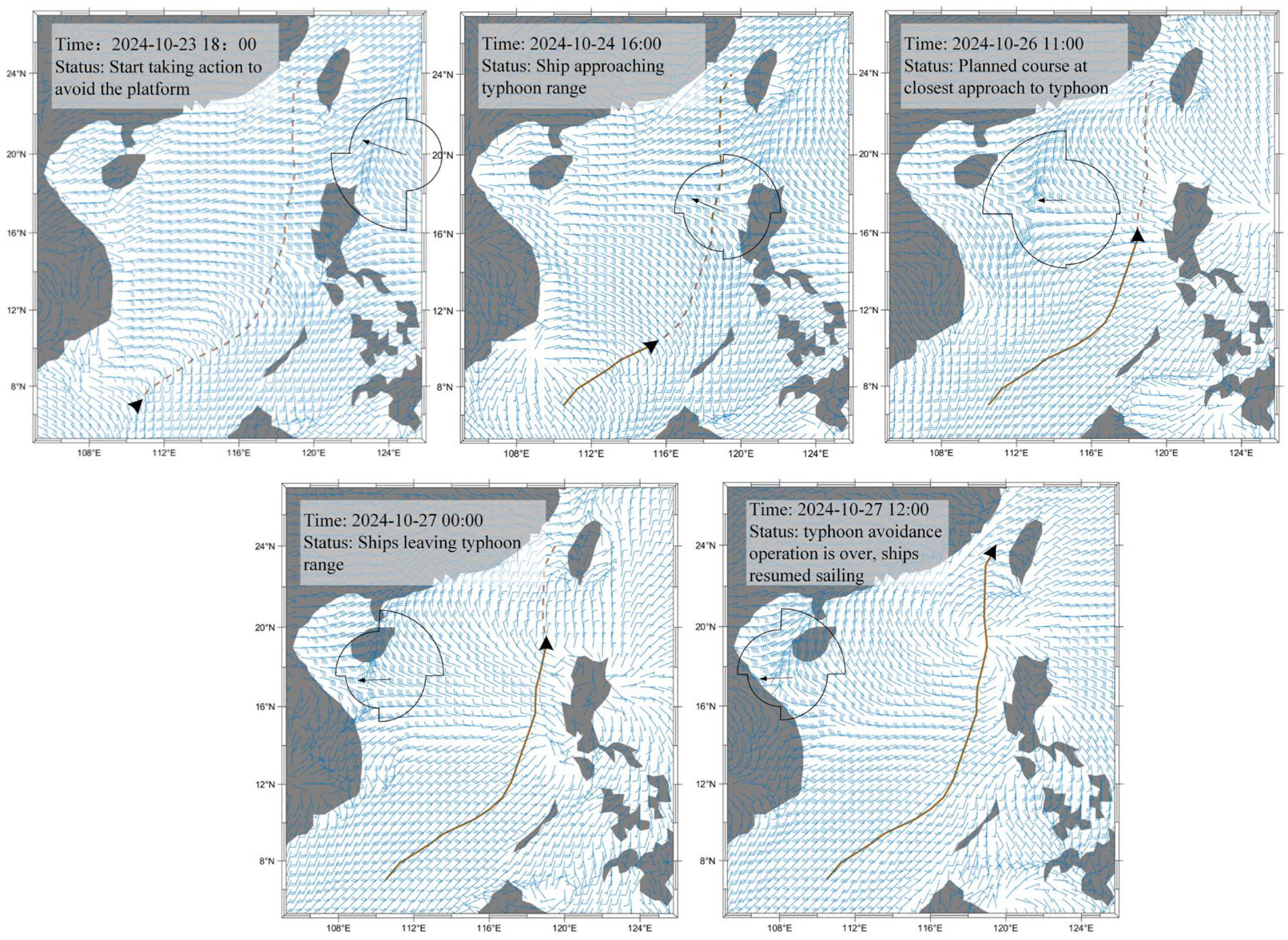
6.2.1. Design of Avoidance Routes

The overall process of ship avoidance is shown in Figure 11. Before the ship safely passes behind the typhoon, the ship needs to update the ship’s course and speed according to the real-time typhoon observation and forecast information as well as the marine meteorological data to maximize the safety of ship navigation.

According to the forecast information of Typhoon TARMI provided by the Japan Meteorological Agency at 15:00 on 23 October, the physical model in Section 4.1 was used to calculate the minimum safe distance for the next hour by hour as the basis of ship avoidance of the typhoon, and three single-objective routes for avoiding the typhoon, namely the shortest time, the lowest fuel consumption, and the lowest risk, and three multi-objective routes combining the three objectives, were designed, respectively. The four avoidance routes, the planned routes, and the reanalyzed path of Typhoon TRAMI are shown in Figure 12. It can be seen that the four types of avoidance routes are all designed to complete the avoidance action from the rear of the typhoon.

The optimization results of the speed of each section of the four typhoon avoidance routes designed in this paper are shown in Figure 13, in which the speed is the actual value of hydrostatic speed after stall calculation. The results show that the overall speed of the shortest avoidance route is the highest, and the speed of the multi-objective avoidance route shows a trend of decreasing and then increasing, mainly because the ship actively reduces its speed when approaching the area of typhoon winds and waves to ensure the safe passage, and at the same time, stalling occurs due to the influence of winds and waves. The lowest fuel consumption typhoon avoidance routes choose to sail in small wind and wave areas, the speed is not greatly reduced, and the overall speed is the lowest among the four routes to ensure low fuel consumption. The lowest risk route avoids the typhoon by adjusting the heading and speed to avoid the area affected by the typhoon’s category seven wind circle. The multi-objective route weighs the three optimization objectives, and its speed is between the lowest fuel consumption, the lowest risk route, and the shortest time route.

A comparison of the optimization results of typhoon avoidance routes is shown in

Table 8. Comparison of navigational indicators by type of route.

	Nearest Distance to the Wind Circle /nm	Time Spent on the Voyage /h	Fuel Consumption/tons	Total Distance /n mile
Planned routes	−88.09	107.88	432.78	1144.06
Multi-target routes	49.19	90.44	515.28	1246.79
Minimum sailing time routes	−6.02	82.05	586.14	1204.34
Lowest Fuel Consumption Route	199.10	180.41	271.58	1233.11
Lowest risk routes	248.62	134.48	345.47	1297.92

; the typhoon reanalysis data were used to verify the effectiveness of typhoon avoidance. The distance between the planned routes and the shortest avoidance routes and the level seven wind circle is less than 0, which indicates that the closest encounter moment between both of them and the typhoon enters into the range of the level seven wind circle, and the distance between them and the level seven wind circle is only −6.02 nautical miles, which also reflects that there is an error in defining the range of the level seven wind circle only by relying on the minimum safe distance. The distance of the shortest avoidance route is −6.02 nautical miles, which also reflects that there is an error in defining the range of the wind circle by relying only on the minimum safe distance, which has some risk. The lowest fuel consumption avoidance routes are designed to avoid typhoons in areas with little wind and waves, while the lowest risk avoidance routes are designed to avoid typhoons in areas far away from the typhoon area, so the closest distance between the two routes and the category seven wind circle is farther away.

Multi-objective and shortest time routes have reduced by 16.17% and 23.94% in sailing time compared with the planned routes, while the lowest fuel consumption and lowest risk routes have increased by 67.23% and 24.66%, respectively. Due to the round-trip avoidance operation, the voyages of the four types of avoidance routes in the process of avoiding typhoons have increased compared with the planned routes, and increased by 8.98%, 5.27%, 7.78%, and 13.45%, respectively. The voyages of all four routes increased compared with the planned routes, and increased by 8.98%, 5.27%, 7.78%, and 13.45%, respectively. The fuel consumption of multi-objective and shortest time avoidance routes increased by 19.06% and 35.43%, respectively, compared with the planned routes. Since the wind and waves during the voyage of the lowest fuel consumption and lowest risk routes are significantly smaller than the other routes, the fuel consumption was also significantly reduced by 37.25% and 20.17%, respectively. The closest distance between the ship and the typhoon center during the simulation of the planned routes is higher than that of the other routes, so the navigation risk value is much higher than that of the four typhoon avoidance routes.

Compared with the other three routes, the sailing time, fuel consumption, and range of the multi-objective avoidance route were reduced by 99.45%, 13.75%, and 4.10%, respectively, compared with the highest index, and the verification using typhoon reanalysis data (path, range of the Class VII wind circle) shows that the multi-objective avoidance route has a closest distance of 49.19 nautical miles to the wind circle, and can safely pass behind the typhoon.

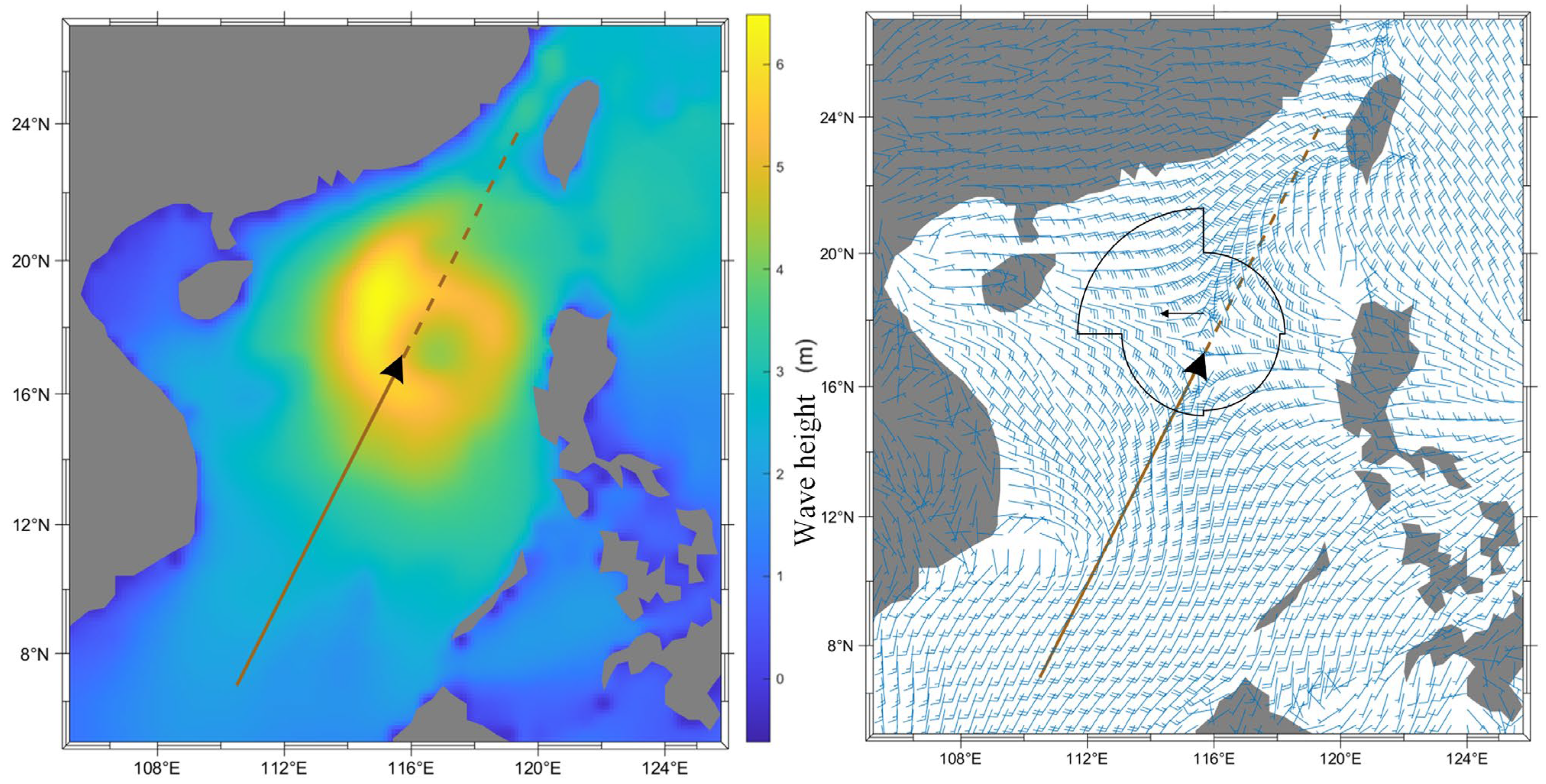
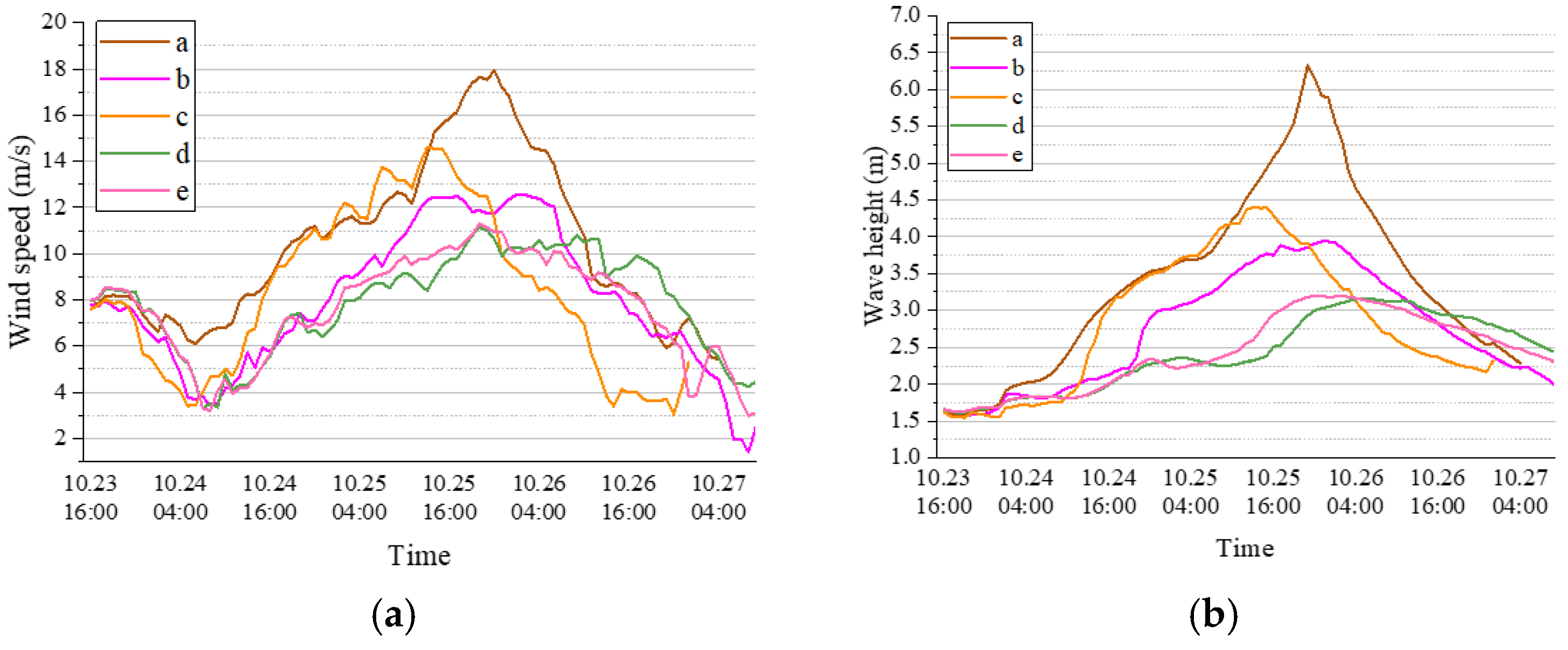
6.2.2. Analysis of Wind and Wave Results of the Typhoon Avoidance Route

In order to analyze the performance of the multi-objective avoidance routes in depth, this section monitors the level of wind and waves encountered by the ship during the voyage. Figure 14a,b demonstrate the changes in wind speed and wave height, respectively. According to the safe ship navigation criteria (wind speed ≤17.2 m/s and wave height ≤5 m), the wind and wave levels of the planned routes are significantly higher than those of the four platform avoidance routes. The wind and wave levels of the four typhoon avoidance routes are all within the safe range. The optimization results of the shortest route in Section 6.2.1 show that it slightly enters the range of the class seven wind circle, which is due to the time resolution of the typhoon reanalysis data used in the simulation (3 h or 6 h) which is interpolated and processed to produce some errors. Nevertheless, the overall wind and wave levels of the shortest route are still higher than those of the multi-target route, while the multi-target route is higher than those of the lowest fuel consumption and lowest risk routes, and the difference in wind and wave levels between the latter two is not significant. Overall, the relationship between the wind and wave levels of the four typhoon avoidance routes and the planned routes is consistent with the route optimization results.

In the above experiment, the ship passes the back of the typhoon smoothly through the scheme of rounding and speed change. In order to describe the whole process of avoiding the typhoon by the avoidance scheme in more detail, this paper plots the sailing process and the rounding and avoidance process of the typhoon in the visualization diagrams of the ship sailing in accordance with the multi-objective avoidance routes in the wind field (as shown in Figure 15) as well as in the wave height field (as shown in Figure 16), respectively.

In this paper, we do not discuss the state of the ship before taking avoidance action and after the ship resumes the planned route, but only discuss the process of avoiding the typhoon. Figure 15 and Figure 16 show the five representative moments of the whole process of avoiding the typhoon, which represent the five states of the process, namely, the moment when the ship starts to take action to avoid the typhoon, the moment when the ship approaches the range of the typhoon, the state of the nearest moment between the typhoon and the ship, the moment when the ship and the typhoon are far away from each other, and the moment when the ship completes the avoidance of the typhoon, which correspond to five subfigures, respectively. The wind plume in the wind field chart indicates the wind direction and wind speed at this time and place. The wave heights are represented by the color hierarchy, and the control scale is on the right side of each wave height chart.

6.2.3. Exhaust Emission Assessment

This paper focuses on the assessment of CO₂ and sulfur oxides emitted during the voyage, which is denoted as SO_X. CO₂ is one of the major greenhouse gases, which absorbs infrared radiation released from the surface and causes heat to be trapped in the atmosphere, which increases the global temperature and is one of the main factors contributing to global warming. And, SO_X accelerates the process of ocean acidification and eutrophication, destroying coral reefs, plankton, and other marine life. High concentrations of SO_X also form acid rain in the atmosphere, causing damage to vegetation and soil in coastal areas. Exhaust emissions are calculated as the product of fuel consumption and emission factor, and the emission factors of CO2 and SOX in the fuels used in this study are 3.173 and 0.0485, respectively, so the results of calculating the emissions of the two types of wastes for each type of route are shown in

Table 9. Exhaust emission statistics for various routes.

	CO2 Emissions/(tons)	SOX Emissions/(tons)	Total Emission
Planned routes	1373.21	20.99	1393.99
Multi-target routes	1634.98	24.99	1659.97
Minimum sailing time routes	1859.82	28.43	1888.25
Lowest Fuel Consumption Route	861.72	13.17	874.89
Lowest risk routes	1096.17	16.75	1112.92

.

Compared with the planned routes, the emissions of CO₂ increased by 261.77 tons and 486.61 tons, and the emissions of SO_X increased by 4.00 tons and 7.44 tons for the multi-objective routes and the shortest time routes, respectively, and the total emissions increased by 273.42 tons and 494.26 tons, respectively. In contrast, the lowest fuel consumption route and the lowest risk route reduced CO₂ emissions by 511.49 and 277.04 tons, SO_X emissions by 7.82 and 4.24 tons, and total emissions by 519.10 and 281.07 tons, respectively, compared to the planned route. This is due to the fact that exhaust emissions are directly proportional to fuel consumption, and the lowest fuel consumption routes and the lowest risk routes have lower fuel consumption, so both have lower CO₂ and SO_X emission indicators than other routes.

6.3. Comparison of the Effect of Improved Algorithms

In order to comprehensively evaluate the integrated performance of the three-dimensional multi-objective ant colony algorithm (3D-ACO) proposed in this paper in complex typhoon avoidance tasks, the multi-objective particle swarm optimization algorithm (MOPSO) and the nondominated sorting genetic algorithm (NSGA-II) were selected as the control algorithms in this paper, and comparative experiments were carried out in a unified oceanic typhoon avoidance planning scenario, and the results are shown in

Table 10. Comparison of the algorithm designed in this paper with other algorithms in terms of the results of each index.

	MOPSO	NSGA-II	3D-ACO
Length of route (nm)	1277.61	1220.91	1246.79
Closest distance to a category 7 wind circle (nm)	15.46	−19.72	49.19
Maximum wind speed (m/s)	16.62	18.92	12.82
Maximum wave height (m)	5.31	5.94	4.41
Average calculation time (s)	54.87	58.66	61.14
convergent algebra	46	51	33

.

In terms of path length, the total route length generated by 3D-ACO was 1246.79 nautical miles, which was slightly shorter than that of MOPSO (1277.61 nautical miles) and slightly longer than that of NSGA-II (1220.91 nautical miles), showing a good balance between voyage economy and platform avoidance safety. In terms of risk avoidance, 3D-ACO performed optimally in several key safety indicators: the minimum distance from the typhoon’s wind circle of category seven was 49.19 nautical miles, which was much better than that of MOPSO (15.46 nautical miles), and NSGA-II even suffered from serious safety risk of its path intruding into the wind circle (−19.72 nautical miles); the maximum wind speed encountered on its path was 12.82 knots, which was significantly lower than that of MOPSO (16.62 knots) and NSGA-II (18.92 knots) ; the maximum effective wave height was 4.41 m, which was also better than MOPSO (5.31 m) and NSGA-II (5.94 m).

The above results show that 3D-ACO can effectively control the ship to operate outside the safe sea area, reduce the risk caused by high wind speed and high wave height, and have a stronger capability of platform avoidance and wind and wave avoidance.

In terms of computational performance, the average computation time of 3D-ACO was 61.14 s, which was slightly higher than that of MOPSO (54.87 s) and NSGA-II (58.66 s), but was still within the acceptable range for practical applications. Meanwhile, the number of convergence generations of 3D-ACO was only 33, which showed higher optimization efficiency compared to MOPSO (46 generations) and NSGA-II (51 generations).

More importantly, 3D-ACO has obvious advantages in dealing with key uncertainties such as typhoon path and wind circle distribution. In this paper, the algorithm incorporated the uncertain typhoon center location and the radius of the class seven wind circle into the path optimization process by introducing probability distribution modeling and improving the stability and robustness of the understanding through the global search and local adaptive mechanism of the ant colony. Compared with other algorithms that are prone to the risk of falling into local optimization in the face of path perturbation or prediction error, 3D-ACO showed stronger flexibility and environmental adaptability, and was able to stably provide high-security routes under a variety of forecast deviation scenarios.

In summary, 3D-ACO shows significant advantages in the safety of platform avoidance, the ability to cope with uncertainty, and the optimization efficiency, which verifies its reliability and practical value as the core method of platform avoidance route planning for ocean-going vessels.

6.4. Model Sensitivity Analysis

In order to further verify the robustness and safety of this paper’s typhoon avoidance model in practical applications, this paper introduces the typhoon forecast path error direction as a perturbation variable to carry out sensitivity analysis. Considering that there is often a certain deviation of the typhoon center position in the actual weather forecast, this paper sets four typical error directions: east, south, west, and north; keeps the error magnitude the same; only changes the offset direction; and compares with the baseline scenario without perturbation.

In each perturbation scenario, the typhoon avoidance path planning algorithm is re-executed and the following key avoidance metrics are recorded: the minimum distance between the ship and the boundary of the actual typhoon’s category seven wind circle (in nautical miles), the maximum wind speed encountered by the ship during its operation along the path (in knots), and the maximum effective wave height Hs encountered along the path (in meters).

Table 11. Table for evaluating the safety of platform-avoidance routes under directional perturbation of path errors.

	Deviation Direction	Min. Distance to Force 7 Wind Circle (nm)	Max. Wind Speed Encounterd (kn)	Max. Significant Wave Height (nm)
Baseline	None	49.19	12.82	4.41
case 1	East	26.54	14.38	4.36
case 2	South	32.87	14.21	3.98
case 3	West	45.42	13.11	3.37
case 4	North	19.35	15.34	4.19

shows the experimental results under different path error directions. From the results, it can be seen that in the baseline case without disturbance, the minimum distance between the ship and the wind circle boundary is 49.19 nautical miles, the maximum wind speed is 12.82 knots, and the maximum effective wave height is 4.41 m, which makes the path the safest. Among the four perturbation scenarios, the westward deviation (Scenario 3) performs the best, still maintaining a distance of 45.42 nautical miles from the wind circle boundary, and the maximum wind speed and wave height are also at a low level (13.11 knots, 3.37 m). Eastward (Scenario 1) and northward (Scenario 4) deviations have a greater impact on path safety: the wind circle boundary distances drop to 26.54 and 19.35 nautical miles, and the maximum wind speeds rise to 14.38 and 15.34 knots, exposing them to more risky sea states. Performance under the southward disturbance (32.87 nautical miles, 14.21 knots, 3.98 m), on the other hand, is in the medium range.

Although some of the perturbation directions lead to a decrease in the safety margin of the path, the path does not enter the typhoon category seven wind circle range in all the scenarios, and the maximum wind speed does not exceed 17.2 knots (the threshold of the category seven wind circle wind speed), and the maximum effective wave height is controlled to be within 5 m, which is still within the acceptable safety zone overall. The sensitivity analysis results show that the typhoon avoidance model in this paper is still able to generate safer typhoon avoidance routes in the face of typhoon path forecast direction errors, especially in the control of wind circle boundaries, wind speed, and wave height avoidance, which reflects the stability and robustness of the algorithm in coping with the input uncertainty. This provides strong support for its application in real shipping decision-making systems.

7. Conclusions

This study estimates the probability of a ship encountering a typhoon by quantifying the probability distribution of the radius of the seven-level wind circle and the center of the typhoon and then designs a risk function. A minimum safe distance constraint is established using a physical model based on the seven-level wind circle calculation. The method is used to optimize the ship’s multi-objective route to avoid the typhoon and achieve the effect of avoiding the typhoon.

In this paper, the classic shipping route in the South China Sea and Typhoon TAMRI are used as examples to study the ship’s route optimization method to avoid typhoons. The results demonstrate that the proposed method effectively avoids areas within a typhoon’s seventh-level wind circle radius and achieves the effect of multi-objective compromise optimization of time-fuel consumption risk.

Since this paper makes assumptions about the probability distribution of the center of a typhoon and the radius of its wind circle of force seven, the probability of a ship encountering a typhoon can be calculated. In future research, further objective analysis of the probability distributions of the two can be conducted; or the accuracy of typhoon forecasts can be further studied to establish a more effective route optimization model for avoiding typhoons. In addition, more comprehensive consideration can be given to the actual various navigation scenarios, and more detailed ship avoidance solutions can be proposed, specifically the following:

(1)

Refining the encounter scenario analysis and model construction: Systematically analyze the various encounter scenarios that may occur between the ship and the typhoon, such as face-to-face encounter, small-angle crossing, large-angle crossing, etc., and construct the decision-making model of avoiding the typhoon for the different encounter modes so as to enhance the adaptability and effectiveness of the avoidance solution.

(2)

Enhancing the scalability and adaptability of the model: Explore the extended application of the platform avoidance model in complex scenarios, such as large-scale multi-vessel collaborative path planning, platform avoidance strategies under double typhoon systems, etc., so as to enhance the applicability of the model in dynamic marine environments.

(3)

Integration of data-driven and intelligent methods: Introduce advanced data-driven techniques, such as deep learning, to adaptively optimize key parameters, such as the probability distribution function of typhoon tracks, to improve the model’s prediction accuracy and generalization ability under different meteorological conditions.

(4)

Exploring real-time applications through satellite data integration: Future work could incorporate satellite remote sensing, AIS vessel tracking, and real-time meteorological datasets to transform the current offline optimization approach into a real-time, adaptive decision-support system, greatly enhancing its value in operational maritime navigation.

References

1. Jewson, S. Tropical Cyclones and Climate Change: Global Landfall Frequency Projections Derived from Knutson et al. Bull. Am. Meteorol. Soc. 2023, 104, E1085–E1104. [Google Scholar] [CrossRef]
2. Shen, Z.; Xu, X.; Li, J.; Wang, S. Vulnerability of the maritime network to tropical cyclones in the northwest pacific and the northern indian ocean. Sustainability 2019, 11, 6176. [Google Scholar] [CrossRef]
3. Ningsih, N.S.; Azhari, A.; Al-Khan, T.M. Wave climate characteristics and effects of tropical cyclones on high wave occurrences in Indonesian waters: Strengthening sea transportation safety management. Ocean. Coast. Manag. 2023, 243, 106738. [Google Scholar] [CrossRef]
4. Szlapczynska, J. Multi-objective weather routing with customised criteria and constraints. J. Navig. 2015, 68, 338–354. [Google Scholar] [CrossRef]
5. Wang, H.; Mao, W.; Eriksson, L. A Three-Dimensional Dijkstra’s algorithm for multi-objective ship voyage optimization. Ocean. Eng. 2019, 186, 106131. [Google Scholar] [CrossRef]
6. Chen, A.; Chen, W.; Zheng, J. Arctic Route Planning and Navigation Strategy: The Perspective of Ship Fuel Costs and Carbon Emissions. J. Mar. Sci. Eng. 2023, 11, 1308. [Google Scholar] [CrossRef]
7. Ma, D.; Ma, W.; Jin, S.; Ma, X. Method for simultaneously optimizing ship route and speed with emission control areas. Ocean. Eng. 2020, 202, 107170. [Google Scholar] [CrossRef]
8. Zhang, G.; Wang, H.; Zhao, W.; Guan, Z.; Li, P. Application of improved multi-objective ant colony optimization algorithm in ship weather routing. J. Ocean. Univ. China 2021, 20, 45–55. [Google Scholar] [CrossRef]
9. Li, Y.; Cui, J.; Zhang, X.; Yang, X. A ship route planning method under the sailing time constraint. J. Mar. Sci. Eng. 2023, 11, 1242. [Google Scholar] [CrossRef]
10. Zaccone, R.; Ottaviani, E.; Figari, M.; Altosole, M. Ship voyage optimization for safe and energy-efficient navigation: A dynamic programming approach. Ocean. Eng. 2018, 153, 215–224. [Google Scholar] [CrossRef]
11. Bijlsma, S.J. On the applications of the principle of optimal evolution in ship routing. Navigation 2004, 51, 93–100. [Google Scholar] [CrossRef]
12. Zhang, L.H.; Zhu, Q.; Liu, Y.C.; Li, S.J. A method for automatic routing based on ECDIS. J. Dalian Marit. Univ. 2007, 33, 109–112. [Google Scholar]
13. Sasa, K.; Chen, C.; Fujimatsu, T.; Shoji, R.; Maki, A. Speed loss analysis and rough wave avoidance algorithms for optimal ship routing simulation of 28,000-DWT bulk carrier. Ocean. Eng. 2021, 228, 108800. [Google Scholar] [CrossRef]
14. Lee, J.S.; Kim, T.H.; Park, Y.G. Maritime Transport Network in Korea: Spatial-Temporal Density and Path Planning. J. Mar. Sci. Eng. 2023, 11, 2364. [Google Scholar] [CrossRef]
15. Wu, L.; Wen, Y.; Wu, D.; Zhang, J.; Xiao, C. Safe-economical route model of a ship to avoid tropical cyclones using dynamic forecast environment. Nat. Hazards Earth Syst. Sci. Discuss. 2014, 2, 4907–4945. [Google Scholar]
16. Wu, L.; Wen, Y.; Peng, S.; Zhang, J.; Xiao, C. Optimizing the routing of ship’s tropical cyclone avoidance based on the numerical forecasts. Nat. Hazards 2013, 69, 781–792. [Google Scholar] [CrossRef]
17. Wu, L.C.; Wen, Y.Q.; Wu, D.Y. Safe-economical route and its assessment model of a ship to avoid tropical cyclones using dynamic forecast environment. Nat. Hazards Earth Syst. Sci. Discuss. 2013, 1, 1857–1893. [Google Scholar]
18. Xiao, Y.; Huang, Y.; Zhang, Y.; Wang, H. Local weather routing in avoidance of adverse sea conditions based on reachability theory. Ocean. Eng. 2025, 315, 119834. [Google Scholar] [CrossRef]
19. Huang, Y.; Ding, X.; Zhang, Y.; Yan, L. T_GRASP: Optimization Algorithm of Ship Avoiding Typhoon Route. J. Quantum Comput. 2022, 4, 85–95. [Google Scholar] [CrossRef]
20. Lee, J.-S.; Kim, M.-K.; Kim, B.-R.; Kim, T.-K.; Lee, C.-Y.; Park, Y.-G. Spatial-temporal big data analysis of ship avoidance patterns during typhoon approaches. Ocean. Eng. 2025, 320, 120316. [Google Scholar] [CrossRef]
21. Sasmal, K.; Miratsu, R.; Kodaira, T.; Fukui, T.; Zhu, T.; Waseda, T. Statistical model representing storm avoidance by merchant ships in the North Atlantic Ocean. Ocean. Eng. 2021, 235, 109163. [Google Scholar] [CrossRef]
22. Liu, L.; Feng, J.; Ma, L.; Yang, Y.; Wu, X.; Wang, C. Ensemble-based sensitivity analysis of track forecasts of typhoon In-fa (2021) without and with model errors in the ECMWF, NCEP, and CMA ensemble prediction systems. Atmos. Res. 2024, 309, 107596. [Google Scholar] [CrossRef]
23. Guo, R.; Yu, R.; Yang, M.; Chen, G.; Chen, C.; Chen, P.; Huang, X.; Zhang, X. Analysis of characteristics and evaluation of forecast accuracy for Super Typhoon Doksuri (2023). Trop. Cyclone Res. Rev. 2024, 13, 219–229. [Google Scholar] [CrossRef]
24. Ren, H.; Liu, H.; Zhang, C.; Sun, X.; Yang, J.; Ke, S. TC-SRNet: Reconstruction and prediction of typhoon high-resolution turbulent fields based on meteorological numerical forecast scale wind fields and deep learning method. J. Wind. Eng. Ind. Aerodyn. 2024, 254, 105885. [Google Scholar] [CrossRef]
25. Zhang, H.; Li, W.; Shi, G.; Desrosiers, R.; Wang, X. A ship trajectory clustering algorithm based on segmentation direction. Ocean. Eng. 2024, 313, 119383. [Google Scholar] [CrossRef]
26. Bai, X.; Xie, Z.; Xu, X.; Xiao, Y. An adaptive threshold fast DBSCAN algorithm with preserved trajectory feature points for vessel trajectory clustering. Ocean. Eng. 2023, 280, 114930. [Google Scholar] [CrossRef]
27. Knaff, J.A.; Sampson, C.R.; DeMaria, M.; Marchok, T.P.; Gross, J.M.; McAdie, C.J. Statistical tropical cyclone wind radii prediction using climatology and persistence. Weather. Forecast. 2007, 22, 781–791. [Google Scholar] [CrossRef]
28. Knaff, J.A.; Sampson, C.R.; Musgrave, K.D. Statistical tropical cyclone wind radii prediction using climatology and persistence: Updates for the western North Pacific. Weather. Forecast. 2018, 33, 1093–1098. [Google Scholar] [CrossRef]
29. Scharfenaker, E.; Yang, J. Maximum entropy economics. Eur. Phys. J. Spec. Top. 2020, 229, 1577–1590. [Google Scholar] [CrossRef]
30. YJ, K. Speed loss due to added resistance in wind and waves. Nav Arch. 2008, 3, 14–16. [Google Scholar]
31. Lu, R.; Turan, O.; Boulougouris, E.; Banks, C.; Incecik, A. A semi-empirical ship operational performance prediction model for voyage optimization towards energy efficient shipping. Ocean. Eng. 2015, 110, 18–28. [Google Scholar] [CrossRef]
32. Walther, L.; Rizvanolli, A.; Wendebourg, M.; Jahn, C. Modeling and optimization algorithms in ship weather routing. Int. J. e-Navig. Marit. Econ. 2016, 4, 31–45. [Google Scholar] [CrossRef]
33. Dorigo, M.; Birattari, M.; Stutzle, T. Ant colony optimization. IEEE Comput. Intell. Mag. 2006, 1, 28–39. [Google Scholar] [CrossRef]
34. Gao, S.; Wang, Y.; Cheng, J.; Inazumi, Y.; Tang, Z. Ant colony optimization with clustering for solving the dynamic location routing problem. Appl. Math. Comput. 2016, 285, 149–173. [Google Scholar] [CrossRef]
35. Zhang, C.; Zhang, D.; Zhang, M.; Zhang, J.; Mao, W. A three-dimensional ant colony algorithm for multi-objective ice routing of a ship in the Arctic area. Ocean. Eng. 2022, 266, 113241. [Google Scholar] [CrossRef]
Figure 1. Framework for estimating the probability of a ship encountering a typhoon.(The arrows in the figure indicate the historical data sources used in the calculation of the probability of a ship encountering a typhoon).
Bdcc 09 00143 g001
Figure 2. Framework for multi-objective route optimization for ship route avoidance.(The arrows in the figure indicate the input of the sailing data from the left figure into the optimization model shown in the right figure).
Bdcc 09 00143 g002
Figure 3. Schematic diagram of the typhoon’s trajectory interval. (The figure indicates that the direction of the two trajectories is shown by the arrows).
Bdcc 09 00143 g003
Figure 4. Guidelines for matching public subfragments of typhoon tracks.
Bdcc 09 00143 g004
Figure 5. Statistical data on the category 7 wind circle of various types of typhoons (the horizontal coordinate indicates the quadrant of the typhoon, the vertical coordinate indicates the size of the radius of the wind circle, and the width of the violin plot represents the degree of concentration of the amount of data). Unit information is added explicitly where missing (for example, axes labels in some graphs showing probability distributions).
Bdcc 09 00143 g005
Figure 6. Schematic diagram of the independent variables.
Bdcc 09 00143 g006
Figure 7. Flowchart of the 3D multi-objective ant colony algorithm.
Bdcc 09 00143 g007
Figure 8. Three-dimensional discretization of navigational space. (The colored points in the diagram are state points, and the state points in each stage form a grid).
Bdcc 09 00143 g008
Figure 9. Infrared satellite cloud image of Typhoon TRAMI (Joint Warning Centre).
Bdcc 09 00143 g009
Figure 10. Infrared satellite cloud image of Typhoon TARMI (Joint Warning Centre).
Bdcc 09 00143 g010
Figure 11. Ship typhoon avoidance flowchart.
Bdcc 09 00143 g011
Figure 12. Route optimization result. (In the legend, a is the path of Typhoon TARMI, b is the planned route, c is the multi-objective route, d is the shortest sailing time route, e is the lowest fuel consumption route, and f is the lowest risk route).
Bdcc 09 00143 g012
Figure 13. Results of speed optimization for various typhoon avoidance routes.
Bdcc 09 00143 g013
Figure 14. Changes in wind speed (a) and wave height (b) during the sailing of a ship according to various routes, with a, b, c, d, and e in the illustration representing planned routes, multi-objective routes, shortest sailing time routes, lowest fuel consumption routes, and lowest navigational risk routes, respectively.
Bdcc 09 00143 g014
Figure 15. Sailing process for typhoon avoidance in multi-objective routes under wind speed field (the time of the voyage and the state of affairs at this point in time are marked in the upper left corner of each diagram).
Bdcc 09 00143 g015
Figure 16. Sailing process for typhoon avoidance in multi-objective routes under wave height field. (The time of the voyage and the state of affairs at this point in time are marked in the upper left corner of each diagram).
Bdcc 09 00143 g016