Helium Speech Recognition Method Based on Spectrogram with Deep Learning

Abstract

With the development of the marine economy and the increase in marine activities, deep saturation diving has gained significant attention. Helium speech communication is indispensable for saturation diving operations and is a critical technology for deep saturation diving, serving as the sole communication method to ensure the smooth execution of such operations. This study introduces deep learning into helium speech recognition and proposes a spectrogram-based dual-model helium speech recognition method. First, we extract the spectrogram features from the helium speech. Then, we combine a deep fully convolutional neural network with connectionist temporal classification (CTC) to form an acoustic model, in which the spectrogram features of helium speech are used as an input to convert speech signals into phonetic sequences. Finally, a maximum entropy hidden Markov model (MEMM) is employed as the language model to convert the phonetic sequences to word outputs, which is regarded as a dynamic programming problem. We use a Viterbi algorithm to find the optimal path to decode the phonetic sequences to word sequences. The simulation results show that the method can effectively recognize helium speech with a recognition rate of 97.89% for isolated words and 95.99% for continuous helium speech.

1. Introduction

The 21st century is the era of the marine economy, with more than 50% of humankind’s clean energy and production materials expected to be obtained from the ocean. Saturation diving is important in the fields of navigation, marine development, marine military, marine rescue, and so on. As such, it is an indispensable part of marine economic development.

Due to the particularity of deep-sea operations, many tasks in the ocean cannot be completed with manned deep-sea submersibles or underwater robots. Divers are required to directly enter the water and be exposed to the deep-sea high-pressure environments to operate. Due to their physiological requirements in deep-sea high-pressure environments, divers need to breathe helium–oxygen mixed gas (He-O₂) during saturation diving. When the diving operation depth is over 50 m, the voices of the divers are obviously distorted. When the depth is over 100 m, the voices of the divers begin to be seriously distorted, and normal speech becomes a bizarre “Donald Duck speech”, called helium speech. This results in communication difficulties between the inside and the outside of a submersible and between divers [1], which affects the deep-sea operations of the divers directly and may even threaten their lives [2]. Therefore, it is urgent to resolve the voice communication of divers in the deep-sea saturation diving context, also known as the helium speech unscrambling problem.

In 1962, the U.S. Navy carried out the first saturated diving experiment using the mixed gas of He-O₂ and observed voice distortion in helium speech communications. They carried out the first quantitative voice analysis and pointed out that the resonant frequency of speech increased in a certain proportion [3]. Subsequently, France implemented the Precontinemt program, and Japan implemented the Sealab program, in which sea-dwelling simulation experiments were carried out. They conducted research and experiments on saturated diving helium speech communication technology [4]. In 1967, Sergeant first reported the helium speech test on the intelligibility of syllable words and the misinterpretation table of consonants considering the use of the mixed gas of He-O₂ at normal atmospheric pressure [5,6]. In 1968, Hollien and Thornpson studied the relationship between the intelligibility of monosyllabic English words and the diving depth (the pressure of the saturated submersible cabin) with the mixed gas of He-O₂. They pointed out that when the diving depth is over 100 m, speech is almost impossible to understand [7].

Further research has shown that it is insufficient to study the mechanism of speech distortion in divers using only the complex acoustic model generated through conventional speech [8]. Lunde used an acoustic transmission line sound channel model to study the resonance peak frequency, bandwidth, and amplitude of helium speech under high pressure. He modified the classical Fant Lindquist formula for resonance peak frequency shift, given the formulas for bandwidth and amplitude shifts [9,10]. Brubaker et al. studied the distortion of English vowels and consonants in a helium–oxygen environment, and the results showed that energy loss occurs in both vowels and consonants in such an environment. However, the energy loss in consonants is more pronounced, which reduces the understanding of helium speech [11].

Although there are various methods for unscrambling or recognizing helium speech, they can be divided into two types in terms of signal processing methods: time-domain processing techniques and frequency–domain processing techniques [12,13]. The former encompasses methods such as tape-recording playback, signal segmentation, and digital encoding. Among these, signal segmentation is the most widely adopted in practice [14]. It can correct the resonance peak frequency distortion of helium speech and even correct the fundamental frequency distortion. Frequency–domain processing usually includes the frequency subtraction method, a speech coder, frequency–domain segmentation processing, the signal analysis method, spectrograms, and so on [15]. Among these, the spectrogram is a relatively effective method.

A spectrogram is a spectrum obtained by processing time-domain signals. It provides a large amount of information related to the characteristics of speech signals, including resonance peaks, fundamental frequency periods, energy, and other parameters. In other words, the spectrogram contains all the original spectral information of the speech signal. Deep learning has powerful learning capabilities that allow systems to process correlations between input features. Introducing deep learning into helium speech recognition can improve the recognition rate of helium speech. The experiment conducted showed that using spectrograms as input features for deep learning systems outperforms one using classical Mel frequency cepstrum coefficients (MFCCs) as input features due to the rich phonetic feature information contained in the spectrogram features [16]. It is worth noting that speech recognition networks can be implemented using fully convolutional networks, which may completely discard the connection layer. Although some feature information may be lost, the speech recognition performance is not reduced. Moreover, fully convolutional neural networks can quickly capture prior information and automatically learn the mapping relationship between input data and target data. This not only improves the accuracy but also shortens the training time [17,18]. Li et al. proposed a helium speech correction algorithm based on deep neural networks (DNNs). In a DNN, the characteristic extraction network extracts the four features of helium speech—formant frequency, formant bandwidth, formant amplitude and pitch—to train the input feature values of the DNN. Each neuron in the neural network layer is connected to all neurons in the previous layer, and each connection has a weight; that is, the input of each neuron in the current layer is the output of the neuron in the previous layer. This algorithm proposed the first machine learning-based helium speech recognition [19]. Reference [20] proposed an adaptive audio-based metric generative adversarial network (AMGAN). In the AMGAN, an adaptive segmentation algorithm and a fusion loss function are used to enhance the ability to learn helium speech features while overcoming the shortcomings of traditional methods in high-pitch correction. This solves the problems of pitch period distortion and formant shift in helium speech and improves the clarity and intelligibility of corrected helium speech. However, due to the limited availability of helium speech data and the lack of supervised information in helium speech recognition training, the learning ability of neural networks is limited.

In order to effectively recognize helium speech based on small samples, we propose a spectrogram-based helium speech recognition method (BS). The helium speech recognition system consists of an acoustic model and a language model with deep learning. The spectrogram features of helium speech, including the fundamental frequency, harmonics, and peaks, are input into the acoustic model, where the helium speech signals are converted to phonetic sequences. In addition, a maximum entropy hidden Markov model is used to decode the phonetic sequence into the word sequence. The main contributions of this work are summarized as follows:

(1)

We extract the time-varying patterns of fundamental frequency, harmonics, and peaks of helium speech from spectrograms, which are used to as the acoustic features of the neural network in the recognition system.

(2)

We introduce deep learning to connectionist temporal classification to form an acoustic model, which can directly learn previously obtained helium speech acoustic features to capture further historical information and future information with stronger robustness and expressive ability.

(3)

A maximum entropy hidden Markov model is employed as a language model to convert the phonetic sequences to word outputs, which can find the optimal path to complete the decoding of phonetic sequences to word sequences and improve the accuracy and fluency of speech recognition.

The rest of this paper is organized as follows. Section 2 describes the helium speech recognition system model based on spectrograms. Section 3 analyzes speech spectrograms and shows the differences and relationships in spectrograms between helium speech and normal speech. Section 4 gives the acoustic model in helium speech recognition. Section 5 presents the language model in helium speech recognition. Section 6 summarizes the helium speech recognition algorithm based on spectrograms. Simulation results are shown in Section 7. Finally, some conclusions are drawn in Section 8.

2. System Model

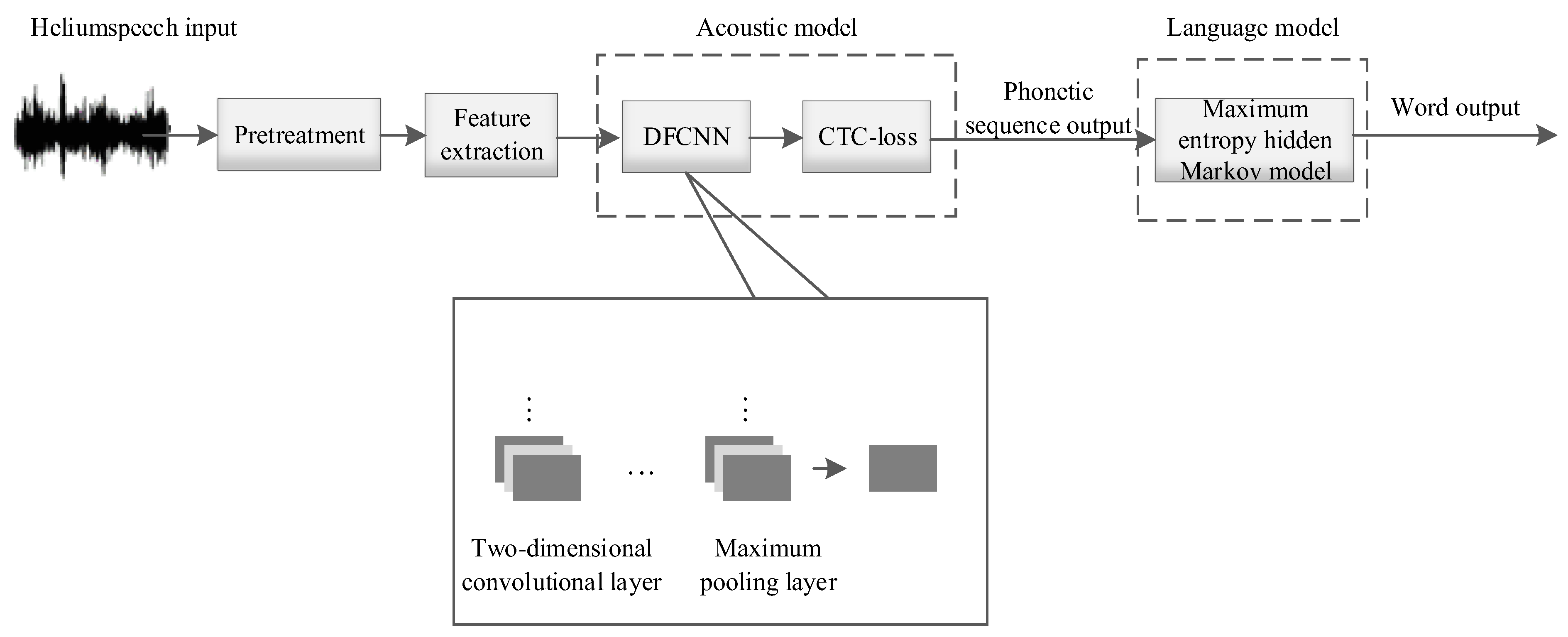
The helium speech recognition system based on spectrograms with acoustic and language models is shown in Figure 1. After pretreatments such as frame segmentation and windowing, the spectrogram features of helium speech are extracted as the input to the acoustic model. The acoustic model consists of a deep fully convolutional neural network (DFCNN) and connectionist temporal classification (CTC); it is used to transcribe sound waveform signals into phonetic sequences. In the language model, the maximum entropy Markov model (MEMM) is used to convert phonetic sequences into words.

3. Helium Speech Spectrogram

The key to the spectrogram-based helium speech recognition method is to extract the spectrogram of helium speech as an acoustic feature for the neural network. A spectrogram is a visual representation that uses a two-dimensional plane to express three-dimensional information. It converts time-domain signals into a three-dimensional expression of time, frequency and energy through a short-time Fourier transform (STFT), represented by the horizontal axis, vertical axis, and color depth, respectively. The darker the color, the stronger the speech energy at that point. The spectrum only analyzes the frequency distribution of a single time signal, with the horizontal axis representing frequency and the vertical axis representing intensity (amplitude or sound pressure), reflecting the energy relationship of instantaneous frequency components. In this study, we use spectrograms to study the dynamic frequency characteristics of helium speech signals over time, including the time-varying patterns of fundamental frequency, harmonics, and peaks. In addition, we can extract the features of plosives, fricatives, and vowels in helium speech through short-pulse straight lines, irregular random patterns, and horizontal bars in spectrograms.

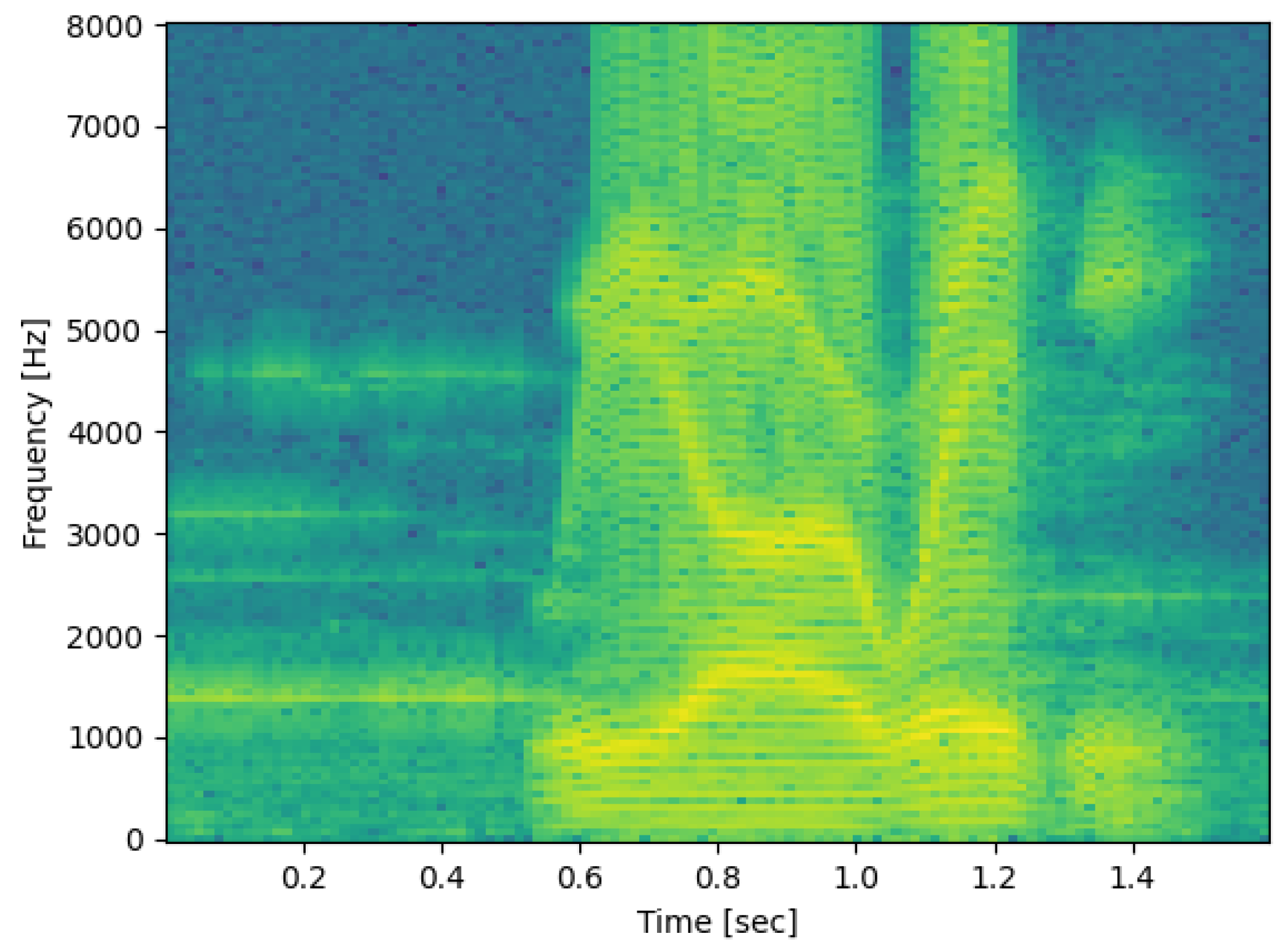
Spectrograms have a small bandwidth in frequency and a large bandwidth in time. Therefore, they require high-frequency resolution and can clearly represent the various harmonics of speech. For example, in the spectrogram of the helium speech phrase “we are ready”, shown in Figure 2, we can clearly see the voice frequency and harmonics. In Figure 2, the frequency range of the low stripes in the horizontal direction represents the pitch frequency. Among these horizontal stripes, some of them are darker in color than other horizontal stripes at the same time. These darker horizontal stripes represent the resonance peak of helium speech. Specifically, multiple darker horizontal stripes may appear locally, forming multiple resonance peaks. 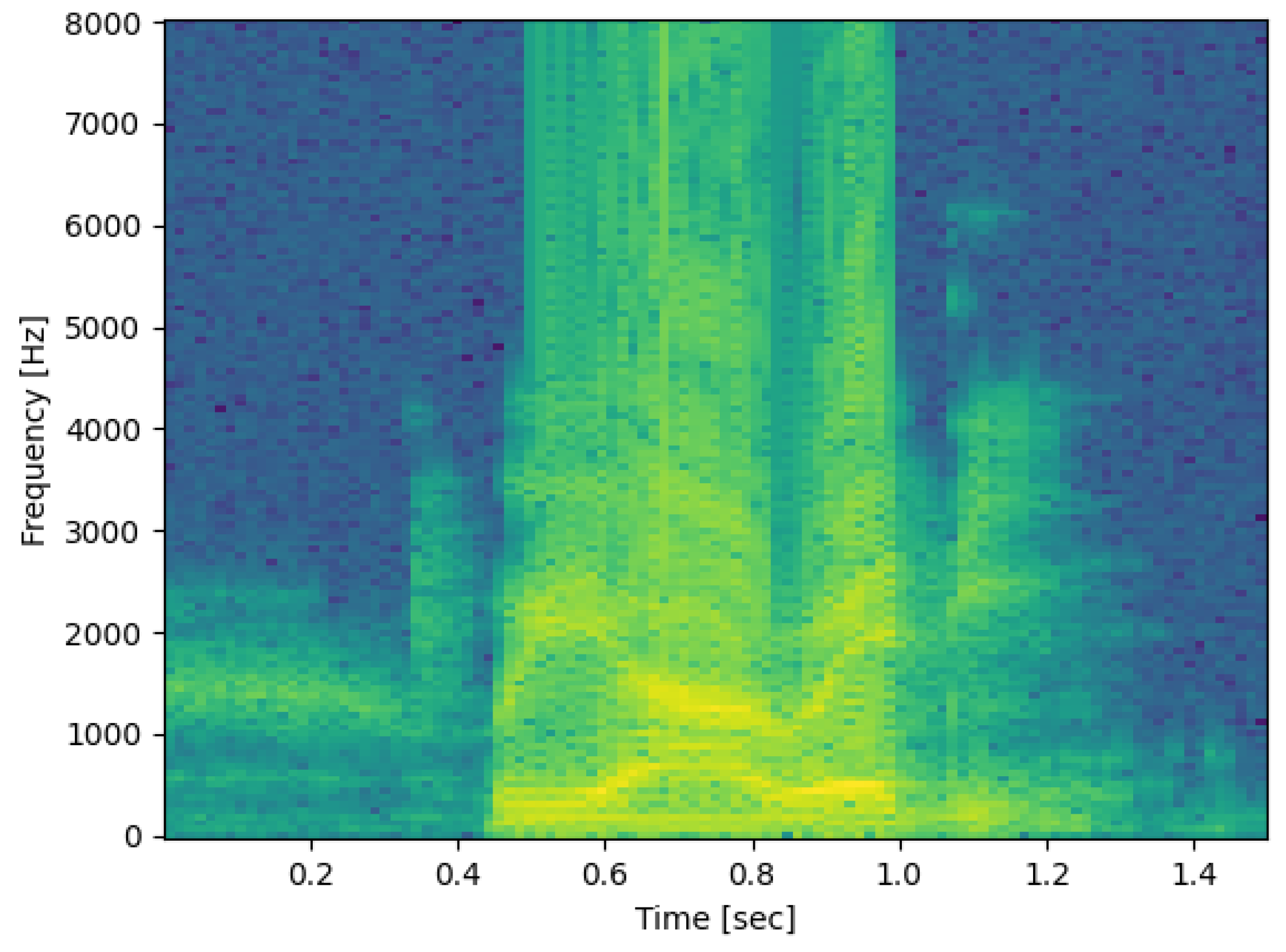Figure 3 shows a spectrogram of the normal speech of the phrase “we are ready” recorded by the same person under a normal atmosphere.

Comparing the spectrograms of speech under a helium–oxygen environment and a normal atmospheric environment, it can be seen that the pitch periods change significantly, and the parameters of the resonance peak characteristics also change, following the rules summarized in relevant studies, such as [18,19,20].

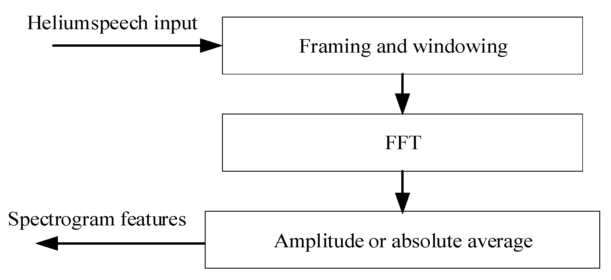
The process of extracting spectrograms is shown in Figure 4. After framing and windowing helium speech in the preprocessing stage, we carry out a fast Fourier transform on each frame signal as follows:

$$S_k\left(e^{j\omega }\right)=\sum _{m=-\infty }^{\infty }s\left(m\right)\cdot w\left(k-m\right)\cdot e^{-j\omega m}$$

(1)

where s(k) is the helium speech signal to be processed, and the window function w(n) is the Hamming window:

$$w(k)=0.54-0.46\mathit{cos}({\displaystyle \frac{2\pi k}{K-1}}),0\le k\le K-1$$

(2)

where K is the length of the Hamming window.

The amplitude or absolute average of the FFT of the helium speech signal, $S_k\left(e^{j\omega }\right),$ is the spectrogram of the helium speech.

4. Acoustic Model in Helium Speech Recognition

The helium speech recognition system uses DFCNN and CTC as acoustic models. Among them, the DFCNN directly learns previously obtained helium speech acoustic features to capture further historical information and future information with stronger robustness and expressive ability. There are convolutional layers instead of fully connected layers in the DFCNN, and each convolutional layer contains a small convolution kernel. We also added a pooling layer after the convolutional layer to represent the long-term correlation characteristics of helium speech better. As the spectrogram becomes smaller and smaller in neural networks, the acoustic features of helium speech will become more and more obvious, and the learning outcomes become better and better.

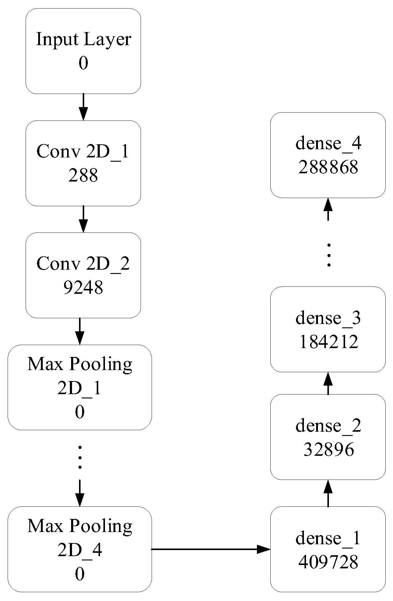
In this paper, our designed DFCNN consists of a total of 54 layers, including 16 two-dimensional convolutional layers and 8 max-pooling layers. A max-pooling layer is inserted after every two convolutional layers, reducing pixel kernels by projecting maximum values onto smaller grids. For DFCNN modeling, the function model.summary (.), from the Keras library on the Python version 3.9 platform, can be used to output the model architecture.

For non-convolutional layers, the number of parameters per layer is given by

Param = (Number of input data dimensions + 1) × Number of neurons

(3)

where Param is the number of parameters per layer. For convolutional layers, the number of parameters per layer is given by

Param = (Length of convolutional kernel × Width of convolutional kernel × Number of channels +1) × Number of convolution kernels

(4)

Figure 5 illustrates the number of parameters for each layer of the DFCNN.

The DFCNN generates the ordered feature sequences from spectrograms, while CTC facilitates the mapping from feature sequences to pinyin sequences. The CTC algorithm is a neural network algorithm for inductive character connectivity, which would enhance the system robustness for texts of varying lengths and alignments. The core of CTC lies in using probability induction to identify a path with the highest probability and derive the outputs. In this work, CTC is used primarily to solve alignment issues between helium speech acoustic features and phonetic sequences, remove repeated characters, silent segmentation markers, and so on.

For different speakers with varying speaking rates, CTC effectively addresses input–output alignment. Let the input audio features be denoted as

x = [x₁, x₂,…, x_T]

(5)

where T is the number of input audio features, and let the corresponding output phonetic sequence be denoted as

$$y=[ y_1,y_2,\dots ,y_N]$$

(6)

where N is the number of output phonetic features. For a given posterior probability $p\left(y|x\right)$, the loss function of CTC is defined as the negative log-likelihood of the posterior probability as follows:

$$Loss\left(x\right)=\sum _{\left(x,y\right)\in D}-\mathit{log}p\left(y|x\right)$$

(7)

where D represents the training set.

To avoid consecutive identical phonetic characters, we introduce a placeholder symbol “−”, which corresponds to “no character” and is removed in the final output. Notably, the alignment between input x and output $y$ is monotonic; that is, when the present input x_t advances to input $x_{t+1}$, corresponding to the next time slot, $y$ may either remain unchanged or move to output $y_{n+1}$, corresponding to the next time slot. Additionally, the input and output follow a multiple-input–single-output relationship.

Typically, CTC follows a recurrent neural network (RNN). For a given input x, the output of the RNN is z = [z₁, z₂,…, z_T]. We denote the feature dimension of x_t as u, and the feature dimension of z_t as v. For each component z_t, we select an element to form an output path l. The space of the output path is denoted as L^T. We define a mapping F that represents the transformation of the intermediate output path. We also need to merge adjacent characters and remove placeholders to obtain the final output $y$. The posterior probability of $y$ to x $p\left(y|x\right)$ equals the sum of probabilities of all valid paths as follows:

$$p\left(y|x\right)={\sum }_{F\left(l\right)=y}p\left(l|x\right)$$

(8)

where $p\left(l|x\right)$ is the posterior probability of path l to x. The calculation of the posterior probability $p\left(y|x\right)$ is detailed in Appendix A.

The CTC-based acoustic model operates independently of language models. When the language application scenarios are changed, we can seamlessly switch the language models. In other words, when the speech content shifts from lifestyle topics to professional topics, CTC can easily exchange language models.

5. Language Model in Helium Speech Recognition

Processing methods for natural language processing are mainly divided into two categories, rule- and statistical-based methods, where the former are often more effective. The language model in our helium speech recognition system is a statistical language model used to convert phonetic sequences to words.

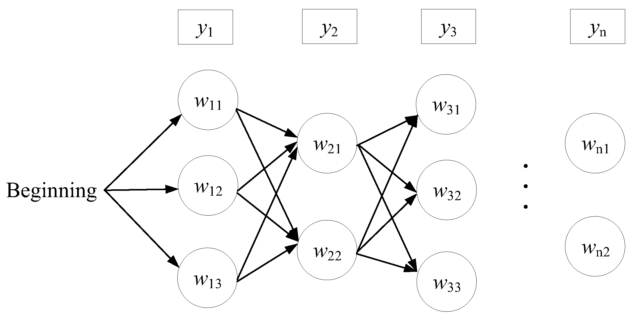
For most languages, such as English and Chinese, each pronunciation can correspond to multiple words, while each word is read using only one sound at a time. In connecting the corresponding words of each pronunciation in an orderly manner, a directed graph can be formed to represent the dependency relationship between phonetic sequences and words, as shown in Figure 6. Suppose the input is the phonetic sequences $y_1,y_2,\dots ,y_N$, the candidate words for pronunciation $y_1$ are w₁₁, w₁₂, and w₁₃, while the candidate words for pronunciation $y_2$ are w₁₁, w₁₂, and so on.

In a statistical language model, according to the Markov hypothesis, the probability of each word appearing is only considered to be related to the previous words, which is called a binary language model. Thus, if S represents a sentence with a string of words w₁, w₂, …, w_N, where N is the length of the sentence, the probability of sentence S being present is given by

$$p\left(S\right)=p\left(w_1,w_2,\dots ,w_N\right)=p\left(w_1\right)p\left(w_2|w_1\right)p\left(w_3|w_2\right)\dots p\left(w_N|w_{N-1}\right)$$

(9)

where $p\left(w_1\right)$ is the probability that word w₁ is present, $p\left(w_N|w_{N-1}\right)$ is the conditional probability that word w_N is present if word w_N−1 is present. According to the law of large numbers, when there are enough statistical measures, these probabilities can be obtained based on word frequency.

In our maximum entropy Markov model (MEMM), we use a maximum entropy model to learn the conditional probability $P\left(s_t|s_{t-1},o_t\right)$ to perform the maximum likelihood estimation under the given training data conditions as follows:

$$P_w(y|x)={\displaystyle \frac{\exp ({\displaystyle {\sum }_i{w}_i{f}_i(x,y)})}{Z_w(x,y)}}$$

(10)

where $s_t$ and $o_t$ represent the state and observation at time t, $Z_w\left(x,y\right)={\sum }_y\mathit{exp}({\sum }_i{w}_i{f}_i(x,y))$ is the normalization factor, w is the maximum entropy model parameter, λ_i denotes model parameters, and $f_i\left(x,y\right)$ is the feature function. Therefore, the conditional probability is presented as

$$P(s_t|s_{t-1},o_t)={\displaystyle \frac{\exp ({\displaystyle {\sum }_a{\lambda }_a{f}_a(o_t,s_t)})}{Z(o_t,s_{t-1})}}$$

(11)

where ${\lambda }_a$ is the learning parameter, $a=<b,s>$, b is the observed feature, and s is the target state. The feature function $f_a\left(o_t,s_t\right)$ is given by

$$f_a\left(o_t,s_t\right)=\left\{\begin{array}{cc}1& if\hspace{0.33em}b\left(o_t\right)\hspace{0.33em}is\hspace{0.33em}true\hspace{0.33em}and\hspace{0.33em}s=s_t\\ 0& otherwise\end{array}\right.$$

(12)

Once the Markov model is trained (i.e., once the transition probabilities from phonetic sequences to words and from words to words are known), we can use the Viterbi algorithm to decode phonetic sequences into words. This decoding process can be taken as a dynamic programming problem, which is essential to finding the path with the highest probability from the starting point to the endpoint in a directed graph. Then, we arrange the probabilities of each step in order of size and set a threshold to exclude paths with low probabilities. This process repeats until the finish line is reached. The final output is the text of the path with the maximum probability.

The Viterbi algorithm takes two inputs: One input is a hidden Markov model, $\lambda =\left(A,B,\pi \right)$, where $A=[a_{ij}{]}_{N\times N}$ is the state transition probability matrix, $B=\left[b_j\right(k){]}_{N\times M}$ is the observation probability matrix, and $\pi =\left({\pi }_i\right)$ is the initial state probability vector. The other input is the observation sequence $O=\left(o_1,o_2,\dots ,o_T\right)$. Then, the output of the conversion algorithm is the optimal path $I^{*}=\left(i_1^{*},i_2^{*}\dots ,i_T^{*}\right)$.

In order to ensure that each word corresponds to the correct phonetic sequences, it is necessary to find the optimal path with the highest probability within the sentence. According to dynamic programming, if the optimal path passes through node $i_t^{*}$ at time t, then the path from node $i_t^{*}$ to end node $i_T^{*}$ must be optimal among all possible paths from $i_t^{*}$ to $i_T^{*}$. Therefore, we only need to find the maximum probability of each local path with state i at time t from time t = 1, until we obtain the maximum probability of each path with state i at time t = T. The maximum probability at time t = T is the probability P* of the optimal path, while the endpoint of the optimal path $i_T^{*}$ is obtained. Afterwards, in order to find each node of the optimal path, we start from endpoint $i_T^{*}$, gradually find nodes $i_{T-1}^{*},\dots ,i_1^{*}$ from back to front, and obtain the optimal path $I^{*}=\left(i_1^{*},i_2^{*}\dots ,i_T^{*}\right)$. In importing the local probability δ and reverse pointer $\psi$, the maximum value of the probability in all individual paths $\left(i_1,i_2,\dots ,i_t\right)$ with state i at time t is given by

$${\delta }_t\left(i\right)={\mathit{max}}_{i_1,i_2,\dots ,i_{t-1}}P\left(i_t=i,i_{t-1},\dots ,i_1,o_t,\dots ,o_1|\lambda \right) i=\mathrm{1,2},\dots ,N$$

(13)

where the recursive formula for δ is

$${\delta }_{t+1}\left(i\right)={\mathit{max}}_{1\le j\le N}[{\delta }_t\left(j\right)a_{ji}\left]b_i\right(o_{t+1}) i=\mathrm{1,2},\dots ,N;t=\mathrm{1,2},\dots ,T-1$$

(14)

The (t − 1)th node of the path with the highest probability among all individual paths $\left(i_1,i_2,\dots ,i_{t-1}\right)$ with state i at time t is given by

$${\psi }_t(i)={\mathit{argmax}}_{1\le j\le N}[{\delta }_{t-1}\left(j\right)a_{ji}] i=\mathrm{1,2},\dots ,N$$

(15)

Thus, we obtain the four steps of the Viterbi conversion algorithm as follows:

(1)

Initialization. ${\Delta }_1\left(i\right)={\pi }_i{b}_i\left(o_1\right),i=\mathrm{1,2},\dots ,N$, ${\psi }_1\left(i\right)=0,i=\mathrm{1,2},\dots ,N$.

(2)

Recursion. For t = 2, 3,…, T, ${\delta }_t\left(i\right)={\mathit{max}}_{1\le j\le N}[{\delta }_{t-1}\left(j\right)a_{ji}\left]b_i\right(o_t),i=\mathrm{1,2},\dots ,N$; that is, the selected node is the one with the highest transition probability from the previous node to the current node. Similarly, for t = 2, 3,…, T, ${\psi }_t\left(i\right)={\mathit{argmax}}_{1\le j\le N}[{\delta }_{t-1}\left(j\right)a_{ji}],i=\mathrm{1,2},\dots ,N$; that is, the path recorded by the reverse pointer is the upper layer starting point with the highest transition probability.

(3)

End Recursion. Choose the state with the highest local probability, that is, $P^{*}={\mathit{max}}_{1\le i\le N}{\delta }_T\left(i\right),{ i}_T^{*}={\mathit{argmax}}_{1\le i\le N}[{\delta }_T(i)]$.

(4)

Backtracking. For t=T−1, T−2,…,1, $i_t^{*}={\psi }_{t+1}\left(i_{t+1}^{*}\right)$, find the optimal path for converting phonetic sequences to words.

(5)

End.

6. Helium Speech Recognition Algorithm

After the optimal path backtracking, the phonetic sequences should be converted to words with the optimal path. Then, helium speech recognition based on spectrograms with deep learning can be summarized as follows:

(1)

Establishing the helium speech database. Establish the isolated helium speech word database and continuous helium speech database separately for training.

(2)

Preprocessing. Preprocess the helium speech data and extract helium speech spectrogram features from the training helium speech.

(3)

Training the helium speech recognition system. Input the extracted spectrogram features into the DFCNN to reduce the feature dimension, and then apply CTC to the features with reduced dimensions to obtain the phonetic output sequence with the highest probability. Finally, input the phonetic sequences into the language model based on statistical methods to obtain the output words.

(4)

Validating the helium speech recognition system. Input the validation dataset into the helium speech recognition system to obtain the word error rate (WER) of the system.

(5)

Testing the helium speech recognition system. Input the testing dataset into the helium speech recognition system to obtain the WER of the system.

In the algorithm above, we only test the proposed helium speech recognition system. In practical use, only steps (2) and (3) are required.

7. Simulation Results

We simulated our helium speech recognition algorithm based on spectrograms. As there is no publicly available helium speech database at present, we used a self-made helium speech database. We selected English as the saturation diving working language for divers. Its reading content mainly includes five sections: common words, article paragraphs, diving technical terms, daily conversations, and technical instructions. The data were collected from divers using helium−oxygen gas during saturation diving to depths of 150 m or so while reading aloud. The recordings were made using high-sensitivity microphones and professional recorders to ensure high audio quality. As saturation divers cannot record in real environments for a long time, the total duration of the dataset was only 108 min, recorded by three divers. These three divers had extensive diving experience and were capable of accurately reading professional terms and technical descriptions. Each diver’s average reading time was approximately 36 min. The dataset was stored in WAV format with a sampling rate of 16 kHz. These data were later segmented into smaller speech fragments for use in speech processing and analysis, facilitating model training and testing. The helium speech database is described in more detail in [20].

During the DFCNN training process, there were 1,603,156 parameters and 1,603,156 trainable parameters. In the experiment, the frame length of the speech data is set to 32 ms, the frame shift was set to 16 ms, and the number of points of the fast Fourier transform was set to 512.

In this paper, we use the word error rate (WER) to measure the recognition rate of the helium speech recognition algorithm as follows:

$$\mathrm{W}\mathrm{E}\mathrm{R}={\displaystyle \frac{Number of error words}{Total number of words}}\times 100\%$$

(16)

Table 1. WERs of isolated words of helium speech in training.

Loss Value	WER% (Training Set)	WER% (Validation Set)	Number of Training Iterations
2.3741	78.9	88.9	5
1.5671	16.6	25.6	10
1.4662	5.0	7.1	15
1.3827	0.0	2.8	20
1.2716	0.0	2.1	25
1.2214	0.0	2.1	30

shows the performances of the helium speech recognition algorithm based on spectrograms (HRABS) in the training process of isolated words of helium speech. As the number of training iterations increases, the loss value gradually decreases and tends to stabilize. Moreover, the WER of the isolated word recognition both in the training set and validation set continuously decreases. From Table 1, we can also see that the WER of the validation set is significantly higher than that of the training set. This is because the spectrogram features of words trained have already been retained in the model.

Table 2. WERs of continuous helium speech in training.

Loss Value	WER% (Training Set)	WER% (Validation Set)	Number of Training Iterations
14.1225	34.8	98.3	1
7.8949	5.1	81.1	4
3.8561	1.2	30.3	8
1.9213	0.0	22.4	12
1.6363	0.0	16.5	17
1.3762	0.0	10.4	24
1.2323	0.0	7.0	26
1.1751	0.0	5.7	30
1.0479	0.0	4.1	31
1.0827	0.0	4.0	35

presents the performances of HRABS in the training process of continuous helium speech. Table 2 shows that the loss value of the model is only reduced to 14.1225 after one round of training, which is high. This is because there were many more training data, about 1000 training data points. As the number of training rounds increases, the loss value gradually decreases, and the WER of word recognition in the training and validation sets also decreases. The training would end when the model loss value tends to stabilize.

We also compared our helium speech recognition algorithm based on spectrograms (HRABS) with a DNN [19] and AMGAN [20].

Table 3. WERs of helium speech unscrambling with different algorithms.

	WER of Isolated Helium Speech Words (%)	WER of Continuous Helium Speech (%)
HRABS	2.11	4.01
DNN	12.64	19.45
AMGAN	8.21	11.67

shows the WERs of the isolated helium speech words and continuous helium speech, respectively, with two different unscrambling algorithms. Those obtained with HRABS are much smaller than those based on the DNN and AMGAN, both in isolated helium speech words and continuous helium speech. In particular, the WER of continuous helium speech unscrambling with the algorithm based on a DNN is close to 20%, which is too high to be used in practice.

Table 4. WERs of continuous helium speech unscrambling for different divers.

	WER of Diver 1 (%)	WER of Diver 2 (%)	WER of Diver 3 (%)	Mean Square Error of WERs
HRABS	4.68	4.63	4.23	0.20
DNN	17.12	19.12	22.12	2.05
AMGAN	10.98	12.34	11.68	0.56

shows the robustness of these two different unscrambling algorithms to different divers. We use the mean square error of the WERs to denote the fluctuation in WERs for different divers. It is clear that these fluctuations of the algorithms based on the HRABS and AMGAN are both much lower than those based on the DNN. This is to say that our unscrambling algorithm and AMGAN both have better robustness to different divers.

To demonstrate the superiority of our proposed system, we also compared it with three other systems: a spectrogram-based helium speech recognition system in which MEMM is replaced with HMM (system-HMM), a spectrogram-based helium speech recognition system in which CTC is replaced with a transformer-based model (TBM) (system-TBM), and a spectrogram-based helium speech recognition system with only CTC and no DFCNN (system-CTC).

Table 5. WERs of spectrogram-based helium speech recognition systems with different algorithms.

	WER of Isolated Helium Speech Words (%)	WER of Continuous Helium Speech (%)
HRABS	2.11	4.01
System-HMM	20.12	25.32
System-TBM	10.44	13.23
System-CTC	14.47	19.84

shows that the performances of the other three algorithms were poor due to a lack of the unbiasedness and robustness of MEMM, a lack of the high flexibility of CTC, or a lack of the feature extraction capability of NND.

From Table 3, Table 4 and Table 5, it can be concluded that the helium speech unscrambling algorithm based on HRABS has better performance and better robustness to different divers.

8. Conclusions

In order to recognize helium speech in the context of saturated diving effectively, we proposed a helium speech recognition method based on spectrograms. This algorithm extracts spectrograms from helium speech as acoustic features, combines a deep convolutional neural network and connectionist temporal classification to construct an acoustic model of helium speech, and then uses a statistical language model to recognize saturated diving helium speech. We evaluated the performance of the helium speech recognition algorithm based on the Python platform. The simulation results demonstrated that the algorithm can effectively recognize isolated words of helium speech with 97.79%, and continuous words of helium speech with 95.99%. It showed excellent performance in helium speech recognition, with significant improvements in clarity and intelligibility compared to traditional methods. These results not only enrich the theoretical foundation in the field of helium speech recognition but also provide effective technical support for practical applications.

However, this study has several limitations. First, the recognition performance of continuous helium speech shows that the recognition algorithm has limited generalization ability. This limitation may affect the model’s ability to generalize under various accents and speaking styles. Additionally, the lack of samples from different regions and cultural backgrounds may reduce the model’s adaptability when processing diverse speech inputs.

To address these issues, future work should focus on enhancing the dataset’s diversity. Strategies include expanding the data collection to include divers from different regions and linguistic backgrounds. Increasing the amount of helium speech data is important. Furthermore, applying state-of-the-art transformer-based models or hybrid CNN-RNNs may improve the generalization ability in accents and intonations. Finally, this study mainly examined the application of spectrograms in helium speech recognition based on a fully convolutional neural network with connectionist temporal classification and a maximum entropy hidden Markov model. Future work could explore the performance of other deep learning models in helium speech correction to identify more optimized solutions. Hopefully, more researchers will conduct in-depth investigations in this field, thus advancing the development of helium speech recognition technology.