Article

From Accuracy to Vulnerability: Quantifying the Impact of Adversarial Perturbations on Healthcare AI Models

School of Computing and Creative Technologies, University of the West of England, Bristol BS16 1QY, UK
*
Author to whom correspondence should be addressed.
Big Data Cogn. Comput. 2025, 9(5), 114; https://doi.org/10.3390/bdcc9050114
Submission received: 17 January 2025 / Revised: 6 April 2025 / Accepted: 23 April 2025 / Published: 27 April 2025
(This article belongs to the Special Issue Big Data Analytics with Machine Learning for Cyber Security)

Abstract

:
As AI becomes indispensable in healthcare, its vulnerability to adversarial attacks demands serious attention. Even minimal changes to the input data can mislead Deep Learning (DL) models, leading to critical errors in diagnosis and endangering patient safety. In this study, we developed an optimized Multi-layer Perceptron (MLP) model for breast cancer classification and exposed its cybersecurity vulnerabilities through a real-world-inspired adversarial attack. Unlike prior studies, we conducted a quantitative evaluation on the impact of a Fast Gradient Sign Method (FGSM) attack on an optimized DL model designed for breast cancer detection to demonstrate how minor perturbations reduced the model’s accuracy from 98% to 53%, and led to a substantial increase in the classification errors, as revealed by the confusion matrix. Our findings demonstrate how an adversarial attack can significantly compromise the performance of a healthcare AI model, underscoring the importance of aligning AI development with cybersecurity readiness. This research highlights the demand for designing resilient AI by integrating rigorous cybersecurity practices at every stage of the AI development lifecycle, i.e., before, during, and after the model engineering to prioritize the effectiveness, accuracy, and safety of AI in real-world healthcare environments.

1. Introduction

According to the WHO, breast cancer remains the most common cancer in women worldwide. In 2022 alone, 2.3 million women were diagnosed with breast cancer, and approximately 627,000 women lost their lives globally. While breast cancer rates are particularly high in developed regions, it is widely spreading across almost every part of the world. Global statistics highlight significant disparities in the burden of breast cancer based on levels of human development. For instance, in countries with a very high Human Development Index (HDI), 1 in 12 women will face a breast cancer diagnosis during their lifetime, with 1 in 71 women dying from it, whereas in low-HDI countries, while only 1 in 27 women is diagnosed with breast cancer, 1 in 48 women will die from it [1]. Therefore, the early detection of breast cancer is crucial in reducing its complications and improving survival outcomes. Due to the growing number of breast cancer cases, electronic health records have drastically grown, which provides an opportunity for producing significant contributions in the domain of healthcare using AI.
AI models have become essential tools in medical diagnostics, automating processes and supporting the detection of diseases such as breast cancer and brain tumors [2,3,4,5,6]. However, the rapid deployment of AI in healthcare applications can be unsafe due to severe cybersecurity threats, which can endanger the accuracy, reliability, and trustworthiness of AI models. Security breaches in healthcare AI systems pose serious risks, potentially leading to harmful clinical decisions and jeopardizing patient well-being. Attackers can exploit vulnerabilities in Deep Learning (DL) models through adversarial attacks to distort their prediction accuracy and reliability [7,8,9,10]. Due to invalid outcomes, these threats can mislead healthcare practitioners and eventually lead to incorrect treatments or unwanted delays for the patients, which can be a matter of life and death [11,12,13].
In DL models, the cross-entropy loss function plays a significant role in classification tasks, tempering which can violate the integrity of a model. The difference between true labels and predicted probabilities of a model can be measured using the cross-entropy loss. It can be exploited to attack the training phase of a model [14]. This function is defined as
J ( θ , X , y ) = 1 N i = 1 N y i log ( y ^ i ) + ( 1 y i ) log ( 1 y ^ i )
where
  • J ( θ , X , y ) is the loss function that evaluates the model’s performance.
  • N represents the total number of samples in the dataset.
  • y i is the true label for the i-th sample ( y i { 0 , 1 } ).
  • y ^ i is the predicted probability for the i-th sample.
  • θ represents a model’s parameters (e.g., weights and biases).
This loss function penalizes incorrect predictions more heavily and serves as the target for optimization during training. However, adversarial attacks take advantage of the gradients of the loss function concerning the input data to create deceptive perturbations [15,16]. This manipulation demonstrates how the core mechanism that enables the model to learn can also be exploited against it.
In this research, we launched and analyzed the impacts of an adversarial threat to a DL model, using breast cancer detection as the case study. Specifically, we developed an optimized DL model based on Multi-layer Perceptron (MLP) to classify breast cancer cells as benign or malignant and subjected it to adversarial testing through the Fast Gradient Sign Method (FGSM) to quantify the real-world risks posed by such attacks. The rest of this paper is structured as follows. Section 2 critically analyses existing research on cybersecurity vulnerabilities in AI models for healthcare applications and gaps in the domain. The materials and methods applied in our study are discussed in Section 3. Section 4 presents the construction process of the proposed classification model, emphasizing the significant techniques applied to optimize its performance. Section 5 demonstrates the application of an adversarial attack on our model, accompanied by a detailed performance evaluation and critical analysis of the results before and after the attack. Section 6 provides the research conclusion with a summary of the findings and future directions.

2. Related Works

Carlini and Wagner [17] discussed how adversarial attacks could bypass even robust classifiers. They emphasized creating defense strategies. This underscores the importance of integrating adversarial training [18] and other approaches to enhance the robustness of the models to ensure that AI systems in healthcare remain reliable, even under adversarial conditions [19]. Evasion, a specific type of adversarial attack, also aims to deceive DL models by modifying input data during the inference stage. However, unlike adversarial attacks that target training data, evasion attacks focus on bypassing the model’s decision-making process during real-time use. For example, an attacker could introduce subtle alterations in biopsy images, allowing malignant samples to evade detection. Xu et al. [20] proposed feature squeezing to minimize the effectiveness of these attacks by simplifying the input features. Yuan et al. [21] suggested the need for adaptive techniques that can advance as threats arise.
Koh and Liang [22] demonstrated that poisoning attacks can compromise the integrity of ML models. Research has also shown that attackers can recover input data, such as medical records, by accessing the outputs of trained models [23]. These vulnerabilities of the DL models bring up serious privacy concerns relating to protecting patients’ confidential data against unauthorized access. The threats to DL models are not just limited to adversarial patterns. There is significant research on the impact and solution of other attacks, such as data poisoning [24], model inversion [25,26], and model stealing [27,28].
Research has been growing in this domain to address these threats using approaches such as differential privacy and homomorphic encryption, but evolving attacks continue to increase in complexity. Moreover, these defenses often involve trade-offs between computational efficiency and model robustness [29]. Madry et al. [18] provided a framework for adversarially robust models, emphasizing the importance of optimizing models under worst-case perturbations. Recent advancements in robust optimization techniques and secure model architectures offer promising directions for future research [30].
Although significant strides have been made in applying DL for life-critical applications, most current research prioritizes performance improvements in the DL models, yet often overlooks the practical cybersecurity risks that can undermine their reliability in clinical environments. Studies like those of Szegedy et al. [31] and Goodfellow et al. [7] have exposed the vulnerabilities of DL models to adversarial attacks, but the practical implications, particularly on optimized and rigorously evaluated DL models designed for healthcare applications, remain largely underexplored. This research addresses this void by developing an optimized breast cancer detection model and subjecting it to adversarial evaluation using FGSM. By focusing on a real-world-inspired attack and demonstrating its tangible impacts, this study went beyond theoretical exploration and offered actionable insights into securing DL models in life-critical applications. This dual focus on performance and security of DL models establishes a novel contribution, paving the way for developing resilient and trustworthy AI-driven healthcare solutions.

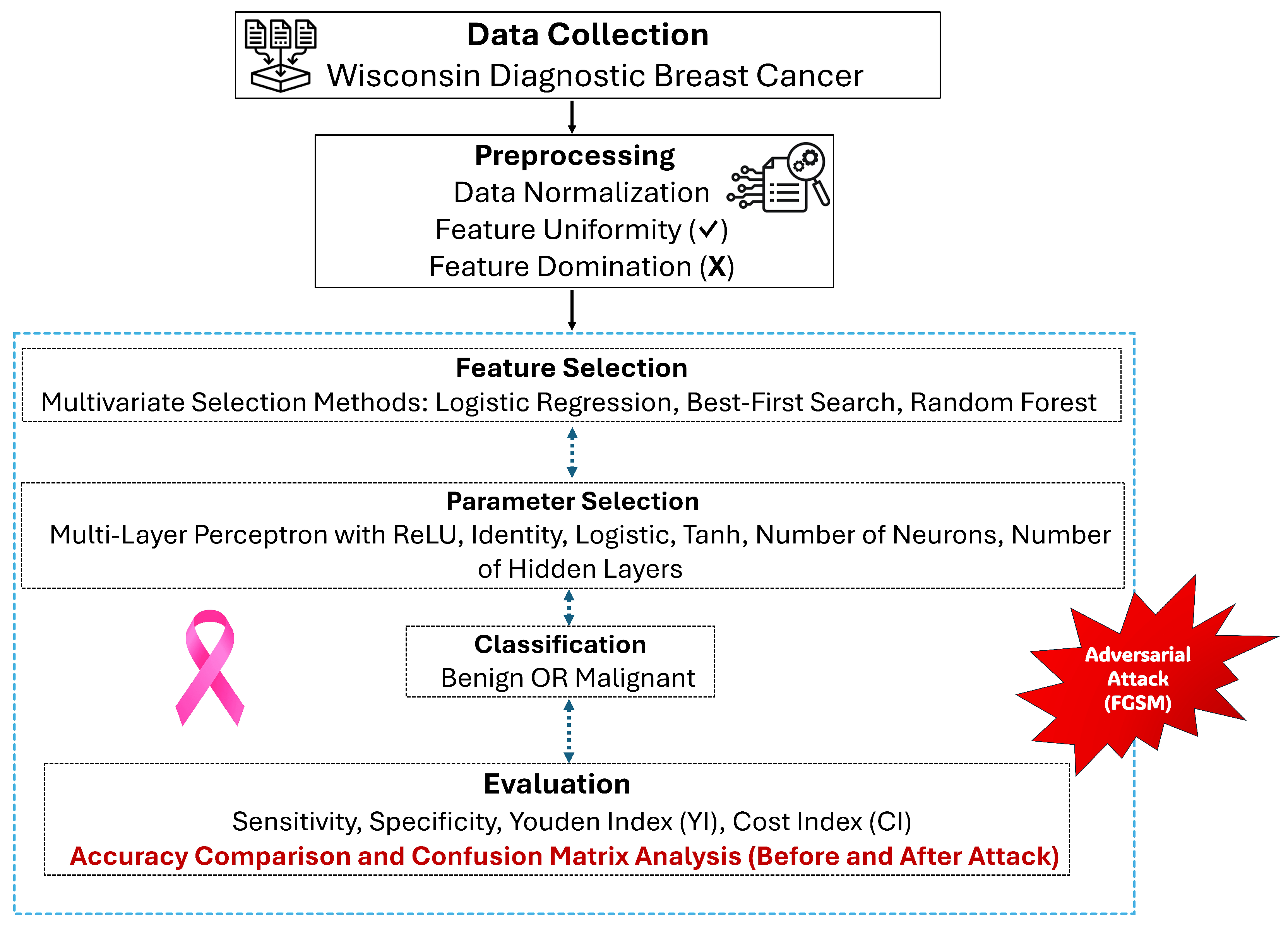
3. Materials and Methods

To investigate adversarial vulnerabilities in medical AI, we adopted the Wisconsin Diagnostic Breast Cancer (WDBC) dataset, sourced from the UCI Machine Learning Repository [32,33]. This dataset includes 569 patient records, each comprising 30 continuous numerical features describing the characteristics of the cell nuclei, along with a unique identifier and a binary label indicating benign or malignant classification. These features include measurements of the cell nuclei size and shape, specifically the mean radius, radius SE, and worst radius, among others, with no missing data. To prepare the dataset, we applied data normalization to scale the features between 0 and 1, ensuring uniformity and avoiding any single feature from dominating the model due to differing scales. The classification threshold for model prediction was set to 0.5, which is the default decision boundary for probability-based classifiers. This threshold was used consistently in our evaluation, and no adjustments were applied for class imbalance. Additionally, the data was then split into training (80%) and testing (20%) subsets using stratified sampling to preserve the class distribution.
We performed feature selection using a multivariate approach to identify the most relevant features that contributed to the model classification performance. All 30 continuous numerical features from the dataset were considered. We identified the 14 most relevant features based on their selection frequency across three methods: Logistic Regression (LR), Best-First Search (BF), and Random Forest (RF). The LR feature selection was performed by evaluating the absolute values of the regression coefficients, where features with the highest absolute coefficients were retained. The RF feature selection was based on feature importance scores obtained from the trained RF model, which ensured that only the most influential features contributing to the classification accuracy were selected. The BF search was applied to evaluate different feature subsets iteratively and identify the optimal combination for classification. From these methods, only the features that were selected by at least two methods, as mentioned in the count column in Table 1, were chosen to reduce the model complexity while maintaining the classification accuracy. The Mean and Standard Deviation (SD) values presented in Table 1 offer descriptive insights and were not used for the feature selection.
An MLP model was developed using Scikit-learn’s MLPClassifier, with a maximum of 1000 iterations, and its performance was rigorously evaluated using the accuracy, sensitivity, specificity, Youden Index (YI), and Cost Index (CI). A grid search was used to determine the optimal combination of the Number of Neurons (NN), Number of Hidden Layers (NHL), and activation functions. The model was optimized by systematically tuning the hyperparameters, including the NN, NHL, and activation functions. Different configurations were evaluated, and the best-performing model was selected based on the accuracy, sensitivity, specificity, Youden Index (YI), and Cost Index (CI). This approach ensured that the optimal configuration was identified through systematic experimentation rather than an automated hyperparameter search.
The model’s vulnerability against the adversarial attack was assessed by measuring the change in its prediction accuracy before and after applying the perturbations. The FGSM attack was conducted multiple times to verify the consistency of its impact on the model performance. Across these trials, the classification accuracy degradation remained stable, confirming the reliability of the adversarial effects. Since the attack’s impact remained consistent across multiple trials, we report a single representative result for clarity, as multiple trials yielded similar classification degradation patterns. For the adversarial attack experiments, we used a Keras implementation of the model. The Keras model was specifically chosen for the adversarial attack experiments due to its compatibility with TensorFlow’s gradient computation framework, which is essential for generating adversarial perturbations. The high-level workflow of the model is shown in Figure 1.

4. The Proposed Model

Our DL model represented in Equation (6) is based on a combination of various activation functions (identity, logistic, tanh, and ReLU) and varying numbers of neurons and hidden layers. The identity activation function, also called the linear activation function, as shown in Equation (2), is one of the simplest forms of activation functions. It directly returns the input value without any modification. The logistic activation function, commonly called the sigmoid function, given in Equation (3), squashes the input values between 0 and 1. The tanh (Hyperbolic Tangent) activation function given in Equation (4) squashes the input to a range between −1 and 1. The ReLU activation function, described in Equation (5), introduces non-linearity by outputting zero for all negative input values while allowing positive input values to pass through without alteration.
f ( z ) = z
f ( z ) = 1 1 + e z
f ( z ) = tanh ( z ) = e z e z e z + e z
f ( z ) = max ( 0 , z )
a L = f ( W L f ( W L 1 f ( W 1 x + b 1 ) + b L 1 ) + b L )
For an input x , W 1 x + b 1 computes the linear transformation of the input x by applying weights W 1 and adding biases b 1 . f denotes the activation function (identity, logistic, tanh, or ReLU) applied element-wise to the result of W 1 x + b 1 . The propagation of the model through the hidden layers is given in Equation (7):
f ( W 2 f ( W 1 x + b 1 ) + b 2 )
W 2 and b 2 denote the weight matrix and bias vector of the second layer, respectively. The term f ( W 1 x + b 1 ) corresponds to the first layer’s output that is passed as input to the second layer after applying the activation function f. This process is repeated iteratively for each hidden layer up to the ( L 1 ) th layer. The computations for the output layer are described in Equation (8). Here, W L and b L represent the weight matrix and bias vector of the output layer. The expression f ( W L 1 f ( W 1 x + b 1 ) + b L 1 ) represents the output of the ( L 1 ) th layer, which becomes the input to the output layer after applying the activation function f.
a L = f ( W L f ( W L 1 f ( W 1 x + b 1 ) + b L 1 ) + b L )
a L is the final output of the model after passing through all the layers, including the activation function f applied to the weighted sums plus biases at each layer. Our model’s design is highly flexible. It enables seamless modifications to the number of layers and neurons, which makes it suitable for a wide range of DL tasks and datasets.

5. Results and Discussion

We used a Scikit-learn-based MLP to implement our model. An MLP function requires adjusting the NHL, NN, type of activation functions, and iterations. We fixed the iterations to 1000 and continuously changed the other experimental parameters. We formed various models using variations of one, two, three, four, and five NHLs with one, ten, twenty, thirty, forty, and fifty NNs using the functions ReLU, Logistic (sigmoid), Hyperbolic Tangent (tanh), and identity activation. We consistently evaluated the performance of the models by measuring the sensitivity, specificity, accuracy, YI, and CI to generate an effective model to classify breast cells into benign or malignant. The 14 selected features were used to build the model using the training dataset. The model was validated using the testing set.
First, we built various sub-models using the identity activation function. The results for the identity activation function with the NHLs and NNs are given in Table 2. No significant difference existed in the sub-models developed using the identity activation function. As shown in Figure 2 and Figure 3, the 2 NHL with 1 NN and 5 NHL with 2 NN showed the highest levels for both the YI and CI. The best model should have the highest YI and lowest CI. Therefore, the identity activation function did not provide suitable results.
We revised the model using the logistic activation function. The results for the logistic activation function with the various NHLs and NNs are given in Table 3. As shown in Figure 4 and Figure 5, the 1 NHL gave a very high YI value and very low CI value for the logistic activation functions. The 2- and 3-NHLs with 10-, 20-, 30-, 40-, and 50-NN sub-models gave very good YI and low CI values. However, the 4 NHL with 20 and 40 NNs gave acceptable values for both the YI and CI indices. The CI values for the 1-, 2-, and 3-NHL configurations exhibited minimal variation, leading to smaller bar heights. Additionally, for 4 NHL, models with 20 and 40 NNs also showed relatively low CI values, which resulted in shorter bars for these configurations. This trend reflected the stability of CI values under logistic activation, where models with these NHL configurations consistently achieved low CI values. The 5 NHL with all the categories of NNs did not perform well with the logistic activation function.
To formulate a module with optimal results, i.e., low cost and high accuracy, we revised our model using the Hyperbolic Tangent (tanh) activation function. The results of the tanh activation function with the various NHLs and NNs are given in Table 4. As shown in Figure 6 and Figure 7, the YI and CI values of the sub-models obtained from the tanh activation function and identity activation function show the same trend, where all the YI values were above 0.9 and the CI values were above 0.4. The 1 NHL with all the categories of NNs showed good performance according to both indices. However, the other NHL sub-models performed very well for all the NN values except 1 NN. The YI values did not show significant differences, but the CI values showed significant differences between the activation functions. The identity and tanh activation functions showed CI values around 0.4.
We further revised our model using the ReLU activation function. The results of the ReLU activation function with the various NHLs and NNs are given in Table 5. The logistic and ReLU activation functions showed similar patterns for the CI values. Figure 8 and Figure 9 show that all the ReLU sub-models showed acceptable YI and CI values, except the models with 1 NN. The CI values for the 1-, 2-, and 3-NHL configurations exhibited minimal variation, leading to smaller bar heights. Additionally, for 4 NHL, models with 20 and 40 NNs also showed relatively low CI values, which resulted in shorter bars for these configurations. This trend reflected the stability of the CI values under the ReLU activation function, where models with these NHL configurations consistently achieved low CI values. Considering the accuracy, sensitivity, specificity, YI, and CI values, the ReLU activation function sub-model performed better than the other models. However, using 1 NN in any combination of NHL and NN is not advisable. Using ReLU, we achieved the best results, namely, accuracy (98.25%), sensitivity (98.53%), specificity (97.83%), YI (96.36%), and CI (47.98%), as shown in Table 5. Though the CI value was slightly high, this was still the best model in terms of sensitivity, specificity, accuracy, and YI because a lower CI results in a significant decrease in other metrics. Therefore, there must be a trade-off between these values to form a DL model with optimal results.
Our model provided the best results with ReLU because it introduced non-linearity into the model while maintaining computational simplicity. This non-linearity enabled the model to learn complex patterns and interactions in the data more effectively than linear or less non-linear activation functions, like identity or logistic. Identity is insufficient for capturing complex data patterns because it does not transform the input so that the model can learn diverse and intricate features. Logistic is a non-linear function but suffers from the vanishing gradient problem, especially when the inputs are far from zero, leading to very slow convergence and potentially poorer performance. Tanh introduces non-linearity and can handle a range of input values better than the logistic function, but it still faces the vanishing gradient issue, particularly for inputs that are very large or very small. ReLU only activates a subset of neurons, leading to more efficient computation and reduced model complexity. This can be particularly beneficial for large datasets. ReLU provided better results for the proposed model with the WDBC dataset because of its ability to introduce efficient non-linearity, mitigate vanishing gradient issues, induce sparsity for feature selection, and handle high-dimensional data effectively. Its superior convergence properties and computational efficiency contributed to improved performance metrics, such as the YI and CI.
In the next phase of our experiment, we evaluated the impact of the FGSM adversarial attack on our breast cancer classification model. For the initial evaluation, we trained and tested a Scikit-learn MLPClassifier, which achieved an accuracy of 98.25%. For the adversarial attack experiments, we used a Keras implementation of the model, which achieved an accuracy of 98%. This minor difference or drop in accuracy was attributed to the inherent randomness in DL workflows, such as weight initialization, data shuffling, and non-deterministic computations. The Keras model was specifically chosen for the adversarial attack experiments due to its compatibility with TensorFlow’s gradient computation framework, which is essential for generating adversarial perturbations. The FGSM attack introduced small, carefully crafted perturbations to the input data that were aligned with the gradient of the loss function to deceive the model into making incorrect predictions. It was expressed as
x = x + ϵ · sign ( x J ( θ , x , y ) ) ,
where
  • x represents the original input.
  • y denotes the true label.
  • ϵ is the perturbation magnitude that controls the attack’s strength.
  • x J ( θ , x , y ) is the gradient of the loss function J with respect to the input x, and θ are the model parameters [34,35].
The value of ϵ was carefully selected to ensure that the perturbation was imperceptible to human observation while still capable of misleading the model. For the implementation, we utilized TensorFlow’s GradientTape to compute the gradients of the loss function with respect to the input features. Our breast cancer classification model was slightly customized, and the FGSM attack was then applied with ϵ = 0.01 , which introduced minor perturbations to the test set inputs. These adversarial examples caused significant misclassifications, where the model’s accuracy dropped to 53%, as shown in Figure 10.
As shown in Figure 11, after the attack, the confusion matrix illustrates the impact of the adversarial attack, showing a clear increase in the overall misclassifications. These errors demonstrate how even small perturbations to the input data could compromise the decision boundaries of the model, leading to incorrect predictions that could have serious consequences in real-world medical diagnostics. These inaccuracies indicate a severe degradation in the model’s reliability for screening purposes. Before the attack, the model achieved a near-perfect accuracy, with a confusion matrix that reflected only minimal errors. Moreover, the accuracy dropped by approximately 45.92%, with the confusion matrix highlighting a substantial rise in classification errors. These results provide practical evidence of adversarial attacks on an optimized DL model in critical applications, where misclassifications can have life-threatening consequences. A malignant cell incorrectly classified as benign could delay critical treatment and worsen patient outcomes, while a benign cell misclassified as malignant could lead to unnecessary procedures that can cause significant psychological and physical distress to the patient. The experimental results provide clear evidence of the vulnerabilities in even an optimized DL model to adversarial attacks. The significant drop in accuracy and the increase in misclassification rates emphasize the critical importance of embedding cybersecurity measures throughout the AI model lifecycle.

6. Conclusions

In this research, we constructed and rigorously evaluated an optimized DL model for classifying breast cancer cells, which achieved an optimal performance in terms of the accuracy, sensitivity, specificity, YI, and CI using the ReLU activation function. However, through the application of the FGSM, we identified that minor and undetectable perturbations to input data could significantly lower the accuracy of our model, and the confusion matrix reflected a substantial rise in misclassifications, which demonstrated the real-world implications of such attacks in medical diagnostics. While DL models offer remarkable medical imaging and diagnostics capabilities, they remain vulnerable to exploitation without appropriate security mechanisms.
To defend against adversarial attacks, practical approaches include adversarial training, where the model is retrained using adversarially perturbed inputs to improve its resilience, and input preprocessing techniques, such as feature squeezing or noise filtering, to reduce the impact of adversarial noise. Additionally, Explainable AI (XAI) methods, like Shapley Additive Explanations (SHAP) and Local Interpretable Model-agnostic Explanations (LIME), can assist in identifying unexpected changes in the feature influence, providing early indicators of adversarial manipulation. Moreover, the cybersecurity approaches must be embedded into the design of AI systems for healthcare. We emphasize the collaborative engineering of AI models with the application of cybersecurity approaches that should be applied during the pre-development (planning), development, and post-development (deployment and maintenance) stages of building AI systems. There is a strong need for creating software development methodologies, policies, and procedures for the effective integration of AI and cybersecurity.
To further strengthen AI security, we also aim to explore the potential of XAI to detect adversarial attacks and enhance model interpretability in our future research. XAI techniques can provide insights into how adversarial perturbations affect DL models, aiding in the development of adaptive defense mechanisms. By leveraging interpretability methods, such as SHAP, LIME, and Saliency Maps, our future research will focus on identifying adversarial patterns and designing countermeasures that improve model resilience against adversarial threats.

Author Contributions

S.B. conceptualized this study; Q.-u.-a.M. managed the data collection and pre-processing tasks. The data analysis and result interpretation were performed by S.B. and Q.-u.-a.M.; the data visualization was led by S.B.; Q.-u.-a.M. reviewed the related works, and both authors identified the research gaps. S.B. designed and implemented the proposed model. S.B. and Q.-u.-a.M. drafted this manuscript. Experimentation was carried out by S.B. and Q.-u.-a.M.; the administrative coordination and documentation support were provided by S.B., with S.B. also serving as the corresponding author. All authors have read and agreed to the published version of this manuscript.

Funding

This research received no external funding.

Data Availability Statement

The dataset analyzed in this study is publicly available and can be retrieved from the source in Reference [32].

Conflicts of Interest

The authors declare no conflicts of interest.

References

  1. WHO. Breast Cancer. 2024. Available online: https://www.who.int/news-room/fact-sheets/detail/breast-cancer (accessed on 21 June 2024).
  2. Hamid, R.; Brohi, S. A Review of Large Language Models in Healthcare: Taxonomy, Threats, Vulnerabilities, and Framework. Big Data Cogn. Comput. 2024, 8, 161. [Google Scholar] [CrossRef]
  3. Mastoi, Q.; Latif, S.; Brohi, S.; Ahmad, J.; Alqhatani, A.; Alshehri, M.S.; Al Mazroa, A.; Ullah, R. Explainable AI in medical imaging: An interpretable and collaborative federated learning model for brain tumor classification. Front. Oncol. 2025, 15, 1535478. [Google Scholar] [CrossRef]
  4. Kumar, V.; Chandrashekhara, K.T.; Jagini, N.P.; Rajkumar, K.V.; Godi, R.K.; Tumuluru, P. Enhanced breast cancer detection and classification via CAMR-Gabor filters and LSTM: A deep Learning-Based method. Egypt. Inform. J. 2025, 29, 100602. [Google Scholar] [CrossRef]
  5. Li, H.; Zhao, J.; Jiang, Z. Deep learning-based computer-aided detection of ultrasound in breast cancer diagnosis: A systematic review and meta-analysis. Clin. Radiol. 2024, 79, e1413. [Google Scholar] [CrossRef] [PubMed]
  6. Ernawan, F.; Fakhreldin, M.; Saryoko, A. Deep Learning Method Based for Breast Cancer Classification. In Proceedings of the 2023 International Conference on Information Technology Research and Innovation (ICITRI), Jakarta, Indonesia, 16 August 2023. [Google Scholar] [CrossRef]
  7. Goodfellow, I.; Shlens, J.; Szegedy, C. Explaining and harnessing adversarial examples. arXiv 2014, arXiv:1412.6572. [Google Scholar]
  8. Akhtar, N.; Mian, A. Threat of adversarial attacks on deep learning in computer vision: A survey. IEEE Access 2018, 6, 14410–14430. [Google Scholar] [CrossRef]
  9. Biggio, B.; Roli, F. Wild patterns: Ten years after the rise of adversarial machine learning. Pattern Recognit. 2018, 84, 317–331. [Google Scholar] [CrossRef]
  10. Veale, M.; Binns, R.; Edwards, L. Algorithms that remember: Model inversion attacks and data protection law. Philos. Trans. A Math. Phys. Eng. Sci. 2018, 376, 20180083. [Google Scholar] [CrossRef]
  11. Tsai, M.J.; Lin, P.Y.; Lee, M.E. Adversarial Attacks on Medical Image Classification. Cancers 2023, 15, 4228. [Google Scholar] [CrossRef]
  12. Muoka, G.W.; Yi, D.; Ukwuoma, C.C.; Mutale, A.; Ejiyi, C.J.; Mzee, A.K.; Gyarteng, E.S.A.; Alqahtani, A.; Al-antari, M.A. A Comprehensive Review and Analysis of Deep Learning-Based Medical Image Adversarial Attack and Defense. Mathematics 2023, 11, 4272. [Google Scholar] [CrossRef]
  13. Finlayson, S.G.; Bowers, J.D.; Ito, J.; Zittrain, J.L.; Beam, A.L.; Kohane, I.S. Adversarial attacks on medical machine learning. Science 2019, 363, 6433. [Google Scholar] [CrossRef] [PubMed]
  14. Bishop, C.M. Pattern Recognition and Machine Learning; Springer: New York, NY, USA, 2006. [Google Scholar]
  15. Kurakin, A.; Goodfellow, I.; Bengio, S. Adversarial examples in the physical world. arXiv 2017, arXiv:1607.02533. [Google Scholar]
  16. Moosavi-Dezfooli, S.M.; Fawzi, A.; Frossard, P. DeepFool: A Simple and Accurate Method to Fool Deep Neural Networks. In Proceedings of the IEEE Conference on Computer Vision and Pattern Recognition (CVPR), Las Vegas, NV, USA, 27–30 June 2016. [Google Scholar] [CrossRef]
  17. Carlini, N.; Wagner, D. Towards Evaluating the Robustness of Neural Networks. In Proceedings of the IEEE Symposium on Security and Privacy (SP), San Jose, CA, USA, 22–26 May 2017. [Google Scholar] [CrossRef]
  18. Madry, A.; Makelov, A.; Schmidt, L.; Tsipras, D.; Vladu, A. Towards deep learning models resistant to adversarial attacks. arXiv 2019, arXiv:1706.06083. [Google Scholar]
  19. Su, J.; Vargas, D.V.; Sakurai, K. One pixel attack for fooling deep neural networks. IEEE Trans. Evol. Comput. 2019, 23, 828–841. [Google Scholar] [CrossRef]
  20. Xu, W.; Evans, D.; Qi, Y. Feature squeezing: Detecting adversarial examples in deep neural networks. arXiv 2017, arXiv:1704.01155. [Google Scholar]
  21. Yuan, X.; He, P.; Zhu, Q.; Li, X. Adversarial examples: Attacks and defenses for deep learning. IEEE Trans. Neural Netw. Learn. Syst. 2019, 30, 2805–2824. [Google Scholar] [CrossRef]
  22. Koh, P.W.; Liang, P. Understanding black-box predictions via influence functions. arXiv 2020, arXiv:1703.04730. [Google Scholar]
  23. Fredrikson, M.; Jha, S.; Ristenpart, T. Model Inversion Attacks That Exploit Confidence Information and Basic Countermeasures. In Proceedings of the 22nd ACM SIGSAC Conference on Computer and Communications Security (CCS ’15), Denver, CO, USA, 12–16 October 2015. [Google Scholar] [CrossRef]
  24. Jagielski, M.; Oprea, A.; Biggio, B.; Liu, C.; Nita-Rotaru, C.; Li, B. Manipulating Machine Learning: Poisoning Attacks and Countermeasures for Regression Learning. In Proceedings of the IEEE Symposium on Security and Privacy (SP), San Francisco, CA, USA, 20–24 May 2018. [Google Scholar] [CrossRef]
  25. Dwork, C.; Roth, A. The algorithmic foundations of differential privacy. Found. Trends Theor. Comput. Sci. 2014, 9, 211–407. [Google Scholar] [CrossRef]
  26. Song, S.; Chaudhuri, K.; Sarwate, A.D. Stochastic Gradient Descent with Differentially Private Updates. In Proceedings of the 2013 IEEE Global Conference on Signal and Information Processing, Austin, TX, USA, 3–5 December 2013. [Google Scholar] [CrossRef]
  27. Tramer, F.; Zhang, F.; Juels, A.; Reiter, M.K.; Ristenpart, T. Stealing Machine Learning Models via Prediction APIs. In Proceedings of the USENIX Security Symposium, Austin, TX, USA, 10–12 August 2016. [Google Scholar]
  28. Orekondy, T.; Schiele, B.; Fritz, M. Knockoff Nets: Stealing Functionality of Black-Box Models. In Proceedings of the IEEE Conference on Computer Vision and Pattern Recognition (CVPR), Long Beach, CA, USA, 15–20 June 2019. [Google Scholar] [CrossRef]
  29. Papernot, N.; McDaniel, P.; Wu, X.; Jha, S.; Swami, A. Distillation as a Defense to Adversarial Perturbations Against Deep Neural Networks. In Proceedings of the 2016 IEEE Symposium on Security and Privacy (SP), San Jose, CA, USA, 22–26 May 2016. [Google Scholar] [CrossRef]
  30. Zhang, H.; Yu, Y.; Jiao, J.; Xing, E.; Ghaoui, L.E.; Jordan, M. Theoretically principled trade-off between robustness and accuracy. arXiv 2019, arXiv:1901.08573. [Google Scholar]
  31. Szegedy, C.; Zaremba, W.; Sutskever, I.; Bruna, J.; Erhan, D.; Goodfellow, I.; Fergus, R. Intriguing properties of neural networks. arXiv 2014, arXiv:1312.6199. [Google Scholar]
  32. Wolberg, W.; Mangasarian, O.; Street, W. Breast Cancer Wisconsin (Diagnostic). 1995. Available online: https://archive.ics.uci.edu/dataset/17/breast+cancer+wisconsin+diagnostic (accessed on 8 March 2024).
  33. Street, W.N.; Wolberg, W.H.; Mangasarian, O.L. Nuclear feature extraction for breast tumor diagnosis. Biomed. Image Process. Biomed. Vis. 1993, 1905, 861–870. [Google Scholar] [CrossRef]
  34. Athalye, A.; Carlini, N.; Wagner, D. Obfuscated gradients give a false sense of security: Circumventing defenses to adversarial examples. arXiv 2018, arXiv:1802.00420. [Google Scholar]
  35. Shafahi, A.; Najibi, M.; Goldstein, T. Adversarial training for free! arXiv 2019, arXiv:1904.12843. [Google Scholar]
Figure 1. Model workflow.
Bdcc 09 00114 g001
Figure 2. Bar chart of the Youden Index using the identity activation function.
Bdcc 09 00114 g002
Figure 3. Bar chart of the Cost Index using the identity activation function.
Bdcc 09 00114 g003
Figure 4. Bar chart of the Youden Index using the logistic activation function.
Bdcc 09 00114 g004
Figure 5. Bar chart of the Cost Index using the logistic activation function.
Bdcc 09 00114 g005
Figure 6. Bar chart of the Youden Index using the tanh activation function.
Bdcc 09 00114 g006
Figure 7. Bar chart of the Cost Index using the tanh activation function.
Bdcc 09 00114 g007
Figure 8. Bar chart of the Youden Index using the ReLU activation function.
Bdcc 09 00114 g008
Figure 9. Bar chart of the Cost Index using the ReLU activation function.
Bdcc 09 00114 g009
Figure 10. Accuracy of the breast cancer model before and after the FGSM attack.
Bdcc 09 00114 g010
Figure 11. Confusion matrices before and after the FGSM attack.
Bdcc 09 00114 g011
Table 1. Summary of the features chosen using various methods.
No.FeatureMeanSDLRBFRFCount
1radius_mean14.133.52YesYesYes3
2texture_mean19.294.30YesYesYes3
3perimeter_mean91.9724.30YesYesYes3
4area_mean654.89351.91NoYesYes2
5smoothness_mean0.100.01YesNoNo1
6compactness_mean0.100.05NoNoNo0
7concavity_mean0.090.08YesYesYes3
8concave points_mean0.050.04YesNoYes2
9symmetry_mean0.180.03YesNoNo1
10fractal_dimension_mean0.060.01NoNoNo0
11radius_se0.410.28NoYesNo1
12texture_se1.220.55YesNoNo1
13perimeter_se2.872.02NoYesNo1
14area_se40.3445.49NoYesYes2
15smoothness_se0.010.00NoNoNo0
16compactness_se0.030.02NoNoNo0
17concavity_se0.030.03NoNoNo0
18concave points_se0.010.01NoNoYes1
19symmetry_se0.020.01NoNoNo0
20fractal_dimension_se0.000.00NoNoNo0
21radius_worst16.27 4.83 YesYesYes3
22texture_worst25.68 6.15 YesYesYes3
23perimeter_worst107.26 33.60 NoYesYes2
24area_worst880.58 569.36 NoYesYes2
25smoothness_worst0.13 0.02 YesNoYes2
26compactness_worst0.25 0.16 NoYesNo1
27concavity_worst0.27 0.21 YesYesYes3
28concave points_worst0.11 0.07 YesYesYes3
29symmetry_worst0.29 0.06 YesNoNo1
30fractal_dimension_worst0.08 0.02 YesNoNo1
Table 2. Model results using the identity activation function.
NHLNNAccuracySensitivitySpecificityYICI
110.96490.95590.97830.93420.450422829
1100.96490.95590.97830.93420.450422829
1200.96490.95590.97830.93420.450422829
1300.96490.95590.97830.93420.450422829
1400.96490.95590.97830.93420.450422829
1500.96490.95590.97830.93420.450422829
210.97370.97060.97830.94890.465122829
2100.96490.95590.97830.93420.450422829
2200.96490.95590.97830.93420.450422829
2300.96490.95590.97830.93420.450422829
2400.96490.95590.97830.93420.450422829
2500.96490.95590.97830.93420.450422829
310.96490.95590.97830.93420.450422829
3100.96490.95590.97830.93420.450422829
3200.96490.95590.97830.93420.450422829
3300.96490.95590.97830.93420.450422829
3400.96490.95590.97830.93420.450422829
3500.96490.95590.97830.93420.450422829
410.96490.95590.97830.93420.450422829
4100.96490.95590.97830.93420.450422829
4200.96490.95590.97830.93420.450422829
4300.96490.95590.97830.93420.450422829
4400.96490.95590.97830.93420.450422829
4500.96490.95590.97830.93420.450422829
510.96490.95590.97830.93420.450422829
5100.97370.97060.97830.94890.465122829
5200.96490.95590.97830.93420.450422829
5300.96490.95590.97830.93420.450422829
5400.96490.95590.97830.93420.450422829
5500.96490.95590.97830.93420.450422829
Table 3. Model results using the logistic activation function.
NHLNNAccuracySensitivitySpecificityYICI
110.97370.97060.97830.94890.465122829
1100.96490.95590.97830.93420.450422829
1200.96490.95590.97830.93420.450422829
1300.96490.95590.97830.93420.450422829
1400.96490.95590.97830.93420.450422829
1500.96490.95590.97830.93420.450422829
210.5965100−22.29387884
2100.96490.95590.97830.93420.450422829
2200.96490.95590.97830.93420.450422829
2300.96490.95590.97830.93420.450422829
2400.96490.95590.97830.93420.450422829
2500.96490.95590.97830.93420.450422829
310.5965100−22.29387884
3100.96490.95590.97830.93420.450422829
3200.96490.95590.97830.93420.450422829
3300.96490.95590.97830.93420.450422829
3400.96490.95590.97830.93420.450422829
3500.96490.95590.97830.93420.450422829
410.5965100−22.29387884
4100.5965100−22.29387884
4200.97370.97060.97830.94890.465122829
4300.5965100−22.29387884
4400.96490.95590.97830.93420.450422829
4500.5965100−22.29387884
510.5965100−22.29387884
5100.5965100−22.29387884
5200.5965100−22.29387884
5300.5965100−22.29387884
5400.5965100−22.29387884
5500.5965100−22.29387884
Table 4. Model results using the tanh activation function.
NHLNNAccuracySensitivitySpecificityYICI
110.96490.95590.97830.93420.450422829
1100.96490.95590.97830.93420.450422829
1200.97370.97060.97830.94890.465122829
1300.96490.95590.97830.93420.450422829
1400.96490.95590.97830.93420.450422829
1500.96490.95590.97830.93420.450422829
210.96490.95590.97830.93420.450422829
2100.97370.97060.97830.94890.465122829
2200.96490.95590.97830.93420.450422829
2300.96490.95590.97830.93420.450422829
2400.96490.95590.97830.93420.450422829
2500.96490.95590.97830.93420.450422829
310.97370.97060.97830.94890.465122829
3100.97370.97060.97830.94890.465122829
3200.97370.97060.97830.94890.465122829
3300.97370.97060.97830.94890.465122829
3400.97370.97060.97830.94890.465122829
3500.97370.97060.97830.94890.465122829
410.97370.97060.97830.94890.465122829
4100.96490.95590.97830.93420.450422829
4200.97370.97060.97830.94890.465122829
4300.97370.97060.97830.94890.465122829
4400.97370.97060.97830.94890.465122829
4500.97370.97060.97830.94890.465122829
510.97370.97060.97830.94890.465122829
5100.96490.95590.97830.93420.450422829
5200.97370.97060.97830.94890.465122829
5300.97370.97060.97830.94890.465122829
5400.98250.98530.97830.96360.479822829
Table 5. Model result using ReLU activation function.
NHLNNAccuracySensitivitySpecificityYICI
110.96490.950.98150.93150.376666747
1100.95610.93330.98150.91480.359966747
1200.96490.933310.93330.9333
1300.95610.93330.98150.91480.359966747
1400.96490.933310.93330.9333
1500.95610.93330.98150.91480.359966747
210.5263100−29.99098664
2100.96490.950.98150.93150.376666747
2200.95610.93330.98150.91480.359966747
2300.97370.9510.950.95
2400.97370.9510.950.95
2500.96490.933310.93330.9333
310.5263100−29.99098664
3100.95610.93330.98150.91480.359966747
3200.96490.933310.93330.9333
3300.96490.950.98150.93150.376666747
3400.96490.933310.93330.9333
3500.97370.9510.950.95
410.5263100−29.99098664
4100.95610.916710.91670.9167
4200.96490.933310.93330.9333
4300.97370.9510.950.95
4400.96490.933310.93330.9333
4500.97370.9510.950.95
510.5965100−22.29387884
5100.97370.97060.97830.94890.465122829
5200.97370.97060.97830.94890.465122829
5300.97370.97060.97830.94890.465122829
5400.96490.95590.97830.93420.450422829
5500.98250.98530.97830.96360.479822829
Disclaimer/Publisher’s Note: The statements, opinions and data contained in all publications are solely those of the individual author(s) and contributor(s) and not of MDPI and/or the editor(s). MDPI and/or the editor(s) disclaim responsibility for any injury to people or property resulting from any ideas, methods, instructions or products referred to in the content.

