Traffic Sign Recognition based on Synthesised Training Data

1. Introduction

Traffic sign classification has been a challenging field in both academia and industry, with the latter receiving high interest. Applications of such systems can range from urban environment understanding, to being an integral part of Advance Driver Assistance Systems (ADAS) [1,2]. Essentially, this task focuses on the fact that each sign consists of a unique combination of shapes, colours and graphics that act as a minimalistic representation of the environment and road conditions, enabling the driver to understand, and possibly prepare, for what he/she may face. Signs are expected to be highly visible to drivers, while signs that represent similar warning/guidance only display a minimum variance between each another. However, due to different environmental conditions, there are cases where the signs appear to be completely distorted, making their inference challenging for humans and machines. Classification shortfalls are mainly caused by the high diversity in the viewpoint of the observer, the lighting of the object, obstacles blocking parts of the sign and the environment in total (for example, the contrast between dusk and dawn), colour fading or even motion blur [3], as seen in Figure 1.

Research on the classification of traffic signs has been seriously hampered by the lack of adequate datasets because data collection of relevant image samples requires time and money. For example, the German Traffic Sign Recognition Benchmark [4] is composed of 43 distinct classes and approximately 50,000 images that were extracted from 10 h of video, with a frame rate of 25 fps. Another instance, where manual work was required to construct the dataset, was an image segmentation and road sign detection and classification system using SVMs for Spanish signs introduced in Timofte et al. [5]. The total number of examples that were included in that work was 35,714, with 153 distinct classes present in the dataset. Other datasets used for recognition or detection include the Swedish roads dataset, obtained from a 20,000-frame video [6], as well as the Belgian traffic sign dataset from KU Leuven Timofte et al. [7]. Because of the different subsets of traffic signs that are used by each dataset, it has been difficult to compare those methods on a common ground.

We believe that the difficulties found in the collection of traffic sign images can be alleviated with the use of synthetically-generated data, without having a significant impact on the accuracy of the classifier. Using as a baseline the fact that the appearance of each sign remains constant in every example and only the environmental and viewpoint factors provide any variations between images, the creation of new training images is targeted towards replicating these conditions. Our approach does not require any real-world data to be used as a guideline by the generator process, with the images created having very high similarity to those from actual observations. Thus, the objective of this method is to maximise the similarity of the generated traffic sign examples with real traffic sign images and without any previous exposure to actual images.

The paper is organised as follows: Section 2 presents an overview of the relative work produced in the field of traffic sign classification and synthetic data generation. Section 3 describes the methodology used to generate a dataset of synthesised images, which will form the training data. Section 4 provides an in-depth analysis of the CNN that was used and the structure that was followed in order to create the network. The details of the experiments alongside the results can be found in Section 5. Finally, Section 6 concludes the presented work and discusses future directions.

2. Related Work

There are several distinct approaches and mindsets for traffic sign recognition, as it has been an active research field in computer vision and machine learning. A typical approach includes computer vision-based techniques for preprocessing the images in such way that the similarity between the classes is minimised, while the similarity within a class should be maximised.

2.1. Early Methods

One of the earliest works in the field was centred on a colour processing system for localising the road sign in the image and later a template matching method to allow real-time extraction of the road sign [8]. Another work that highlights some of the limitations of those methods, was an attempt to utilise an optical filter as the systems’ capacity was highly restricted and, therefore, a large amount of data remained unused [9]. It is possible to categorise traffic sign recognition in different aspects, but one of the most accepted first stage categorisations is to split sign recognition into two categories, Support Vector Machines (SVMs) and learned-features classification methods. A support vector machine is primarily partnered with the use of Histogram of Oriental Gradients (HOG) features [10,11] or with the use of a Gaussian kernel. However, all these approaches include a common image analysis as a preprocessing stage, which incorporates colour thresholding and shape detection, varying little between the methods. The notable advantage of using SVMs compared to other classification methods is the fact that they are easier to train and they are additionally less prone to over-fitting as regularisation is used. Thus, even when the number of attributes is larger than the number of observations, the kernel parameters (if tuned properly) do not allow over-fitting to occur. By creating an SVM that is independent of the dimensionality of the feature space, while being dependent on the margin, they become closely related to the regularisation parameters used.

2.2. Deep Learning Methods

The adaptation of deep learning methods in computer vision tasks has enabled the creation of powerful learned feature classification systems that are empowered by large datasets, aiding towards discovering descriptive class features. One of these first systems was introduced in Cireşan et al. [12] and described a method that combines the outputs of multiple deep neural networks, called Multi-Column Deep Neural Networks (MCDNN). Although kernel filters are used in the same way as seen in CNNs, the essential difference is the use of MaxPooling layers [13] instead of sub-sampling. The chosen structure is based on convolution layers in combination with the MaxPooling layers in which examples are only down-sampled by one pixel. The final results are calculated based on averaging the outputs, produced by every neural network incorporated in the system’s structure. The averaging of single network outputs for this task follows the same principle as described by [14], Meier et al. [15]. Through experiments made on digit recognition, that averaged the outputs of multiple DNN, this allowed the method to generalise better on the test set, albeit the limitations existing in terms of the number of data examples. The accuracy of this approach achieved recognition rates that were ranked better than the average human with the MCDNN performing at 0.9946 accuracy, while a single DNN attained 0.9852 with a margin of $\pm 0.15\%$. A full overview of the models can be found in

Table 1. Accuracy rates (%) of different methods used for traffic sign classification. MCDNN, Multi-Column Deep Neural Networks.

Method	Accuracy
Spatial transform/inception [16]	99.98%
MCDNN [12]	99.46%
Human observations (best)	99.22%
Human observations (average)	98.84%
Multi-scale CNN [3]	98.31%
Random forests [10]	96.14%
LDA and HOG [4]	95.68%

.

Although the MCDNN has shown improvement from other systems, its size and high computational needs constitute it a voluminous implementation for a task that has only a limited degree of complexity with only limited gains in terms of accuracy and less generalisation power, as the model depends on a very high number of parameters that can lead to over-fitting the dataset. An alternative technique as suggested by Jin et al. [17] is the utilisation of a hinge loss cost function similar to the one that is used to train margin classifiers (SVMs). In such systems, the main strategy is to maximise the margin while minimizing the average loss. Therefore, the basic element would be the introduction of a loss function where the penalty is proportional to the predicted labels’ “distance” from the margin boundary between the classes. In this work, the learning stops when the margin is above zero and the training example has been rightfully classified. On the other hand, if the margin is not big enough or the training example has been incorrectly classified, the learning procedure continues. This can be viewed in Equation (1), where y represents the actual label of the example and $\widehat{y}$ represents the predicted label.

$$cost=I(y>0)·max(0,1-\widehat{y})+I(y<0)·max(0,1+\widehat{y})$$

(1)

Despite the aforementioned accuracy improvements, the system that currently suggests the best solution was presented by Haloi [16]. The novelty of this work is that the network includes spatial transformer layers and an inception module that is used to extract local and global features from images. The results of this method were evaluated on the GTSRBdataset and achieved a state-of-the-art accuracy rate of 99.98%. A modified version of GoogLeNet/Inception [18] was used for this task in combination with spatial transformer layers. Although the spatial transform layer was used to learn active transformations, methods for ensuring avoidance of over-fitting, such as an enlargement of the dataset, were not explored fully. This can provide enhancements not only to the dataset that is used, but also to the generalisation of the system to similar classes of different datasets, as the model has learned the most descriptive features and, therefore, is invariant to information that is specific to the data. An example of this is the difference in fonts of speed limits between countries (given that in most cases, the sign remains round) or the change of colour in the background (white to yellow).

3. Generation of Synthetic Training Data

In this section, we discuss the details of various templates and how they are used to produce synthetic training images of these samples under a range of different viewing and illumination conditions.

3.1. Resources

For the purposes of this work, the basic templates that were used were acquired from the YouGov website [19]. From these, the fifty most significant and common classes selected can be seen in Figure 2. The three main categories are:

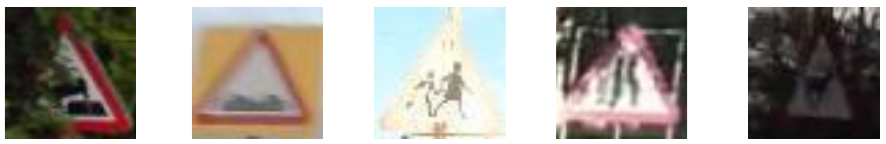
• Warning signs with their characteristics being their triangular shape, with red borders.
• Regulatory signs, which are usually found to have a circular shape, with varying colours (direction indicators or vehicles restrictions).
• Speed limits, which are circular with a red lining (for maximum speed), or blue (minimum speed).

The second set of resources is composed of 1000 images from British roads (and a small portion of general examples from other countries), which will represent the background. There were 500 examples of urban areas and roads, while the other half of the background samples depicted rural environments. This separation took place in order to contemplate the different environments where a traffic sing can be spotted. Additionally, some sign classes are more probable to be observed in rural areas, such as wildlife warning signs. On the contrary, intersection warnings may be more appropriate for urban environments. In our implementation, signs were generated for all 1000 background images without taking into account the probability that a class may be more suited for a specific scenario.

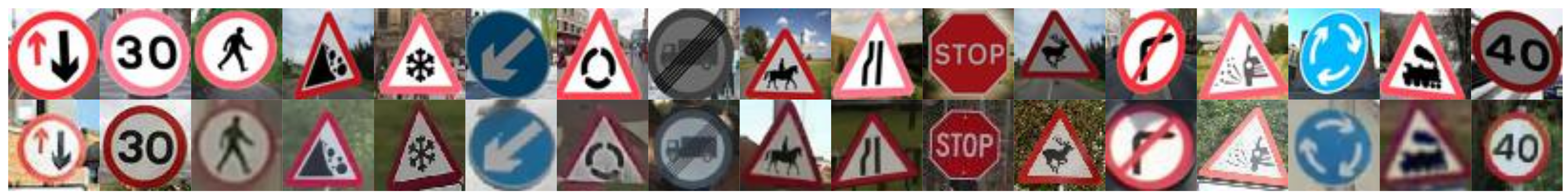
3.2. Generating Novel Training Images from Templates

The initial step of our pipeline is the segmentation of the traffic sign from its background. The equation used to extract the sign is formally written in Equation (2), for the left border, and Equation (3), for the right, which correspond to each row of pixels (yi) in the image. The threshold values were empirically chosen from tests and experiments that were made in order to minimise the number of non-foreground pixels that were obtained during the segmentation of the sign. Programmatically, pixels are considered one dimensional (grey), if they show a difference of lower than 15 between each possible product from the subtraction of two channels. Under other circumstances, this difference would be too great for a variety of colours. However, because signs are assigned with bright colours, in order for them to be distinguishable in a plethora of environments, the assumption of a large channel difference yields satisfying results. The same approach is also applied to the second part of the process where each pixel is compared with its neighbour to find where a large variation exists. A good indication for a pixel being a border pixel of the sign would be the difference in one (or more than one) of its channels compared to the pixel that is next to it.

$$\begin{array}{c}\hfill leftborder=(x_j,y_i):{\alpha }_{(x_j,y_i)}=\left\{\begin{array}{c}|r_{x_j,y_i}-g_{x_j,y_i}|\ge 15\hfill \\ |r_{x_j,y_i}-b_{x_j,y_i}|\ge 15\hfill \\ |b_{x_j,y_i}-g_{x_j,y_i}|\ge 15\hfill \end{array}\right.,where:\begin{array}{c}|r_{x_j,y_i}-r_{x_{j-1},y_i}|\ge 20,or\hfill \\ |b_{x_j,y_i}-b_{x_{j-1},y_i}|\ge 20,or\hfill \\ |g_{x_j,y_i}-g_{x_{j-1},y_i}|\ge 20\hfill \end{array}\\ \hfill forevery0\le y_i\le im{g}_{height},and1\le x\le im{g}_{width}\end{array}$$

(2)

$$\begin{array}{c}\hfill rightborder=(x_k,y_i):{\beta }_{(x_k,y_i)}=\left\{\begin{array}{c}|r_{x_k,y_i}-g_{x_k,y_i}|\ge 15\hfill \\ |r_{x_k,y_i}-b_{x_k,y_i}|\ge 15\hfill \\ |b_{x_k,y_i}-g_{x_k,y_i}|\ge 15\hfill \end{array}\right.,where:\begin{array}{c}|r_{x_k,y_i}-r_{x_{k-1},y_i}|\ge 20,or\hfill \\ |b_{x_k,y_i}-b_{x_{k-1},y_i}|\ge 20,or\hfill \\ |g_{x_k,y_i}-g_{x_{k-1},y_i}|\ge 20\hfill \end{array}\\ \hfill forevery0\le y_i\le im{g}_{height},andim{g}_{width}\ge x\ge 1\end{array}$$

(3)

Once the template is stored in an RGBA format, the affine transformation is applied [20]. This method is used to represent both changes in the rotation and different scales of the sign. Affine transformation has been a standardised technique for producing the illusion created by non-ideal camera angles that are focused on filming specific objects [21]. Geometric distortions are an essential aspect of real examples, as the position of the camera is very likely to produce perspective irregularities while altering the entire scene. The three main uses in this system is the scaling, translation and rotation functions that it provides. Their formal equation can be found in Equation (4). Affine transformation falls into the class of linear 2D geometric transformations in which variables in the original image (such as the colour space values of a pixel P(x, y)) are linked to new variables (for pixel P’(x’, y’)). Therefore, the pixel grid of the image is deformed and mapped to a destination image. For this work, twenty different transformations were used, all based on three significant points in the image. The first point is located close to the start of the axis at one tenth of both the height and the width or alternatively in some instances, at the right side of the image. This determines the shearing of the final image, based on the point that is assigned after the transform is performed. Secondly, the other two points are primarily used for both the rotation and scaling of the image. One is placed in the middle at the top of the image. The second of the two is defined as in the middle of the left side, or the equivalent in some cases, at the right side. All twenty distinct affine transforms are applied to each image class and are stored in files in a directory that is based on the sign to which the transformation was applied.

$$\left[\begin{array}{c}{x}_2\\ y_2\end{array}\right]=A\times \left[\begin{array}{c}{x}_1\\ y_1\end{array}\right]+B$$

(4)

Next, the system computes the average and the Root Mean Square (RMS) brightness of the pixels in the image. This is based on the assumption that the RMS could only be bigger than or equal to the average, which will relate to a higher number assigned to the brightness of the image. However, considering the average pixel values, the image may be assigned a brightness value that is not entirely representative. This might be due to the fact that a minority of pixels include values that are in the borders of the distribution [22] and thus tempering with average value. A possible method to overcome the problem is by utilising the median value. Nonetheless, it has been observed that this difference was beneficial for the method as it was effectively representing variations that are shown in natural settings and the discrete material with which the sign is made. Therefore, in order to preserve a portion of the image noise that is seen in real-world photos, the average and the root mean square values are better suited.

In addition to the average and RMS values, two different approaches are used for understanding the brightness. The first uses a grey-scaled version of the image and computes the average and RMS pixel values. This is considered a standardised method, as the luminance in this instance is defined as the single dimensional image, without the use of the information from any of the other three image channels. An alternative method is the utilisation of the HSPcolour model [23]. The major difference from other colour models such as HSV (which uses the V component to demonstrate the brightness as the maximum value from the RGB channels) or HSL(with L being the average of the maximum and minimum value from the RGB channels), is the fact that it includes the degree of influence of each RGB channel. The equation used for the conversion can be seen in Equation (5), in which the constants represent the extent to which each colour affects the pixel’s luminance.

$$brightness=\sqrt[]{0.299\times R^2+0.587\times G^2+0.114\times B^2}$$

(5)

The same process is also applied to the image with the RMS and average values computed for the 1D image and the perceived brightness. At this stage, all the necessary values have been identified for both the background and foreground; therefore, the margin of the two is calculated as the absolute difference of their respective values. Then, in order to find the brightness that the sign needs to be adapted to, the margin is divided by a ratio that is based on maximising the similarity of all the image features while adding colour distortion to represent background conditions. For measuring similarity and for testing the thresholds, the images were segmented in ten distinct regions. For each region, a histogram was plotted. The histograms were later compared with their equivalent regions at the sign and at the background, as it was found that the best results (histograms that maximised the similarity with the foreground and background images) came with the use of the thresholds selected for each category. The outcome for each approach is depicted in Figure 3.

As a final step, the system stores the image by applying the new illumination that was found through using an enhancer function. There are examples in which this automated procedure was deemed insufficient and the distortions overshadowed the image features. The generated signs are revised with a set of threshold values to segment valuable examples from others that otherwise could not be used. The data separation function considers both cases in which the traffic sign may be black and white. In the instance of a grey sign, an additional function is used to store the file paths of every image that is grey. This is achieved by calculating the difference between all the individual channels on the average pixel value of the image and reassuring that the margin is lower than one. Coloured sings are judged based on the difference between the RGB values. However, conditional independence is assumed between the three relationships, as for example a bright red image will have a great margin when comparing the red and blue channel, but the difference may be less than one in the case of blue and green channels.

The last step of the synthetic example generator is the blending of the background and foreground. This action is performed by a transitional combination of the traffic sign with the background, while also creating a blending effect at the border of the sign for realistic representations of the environmental effects on the object. The bordering pixels are manipulated in a way that the opacity is periodically decreased, and therefore, the final RGB values are changed to an intermediate result between the actual sign and the colours of the background. Final images are resized to 48 × 48 in order to minimise the divergence from actual images.

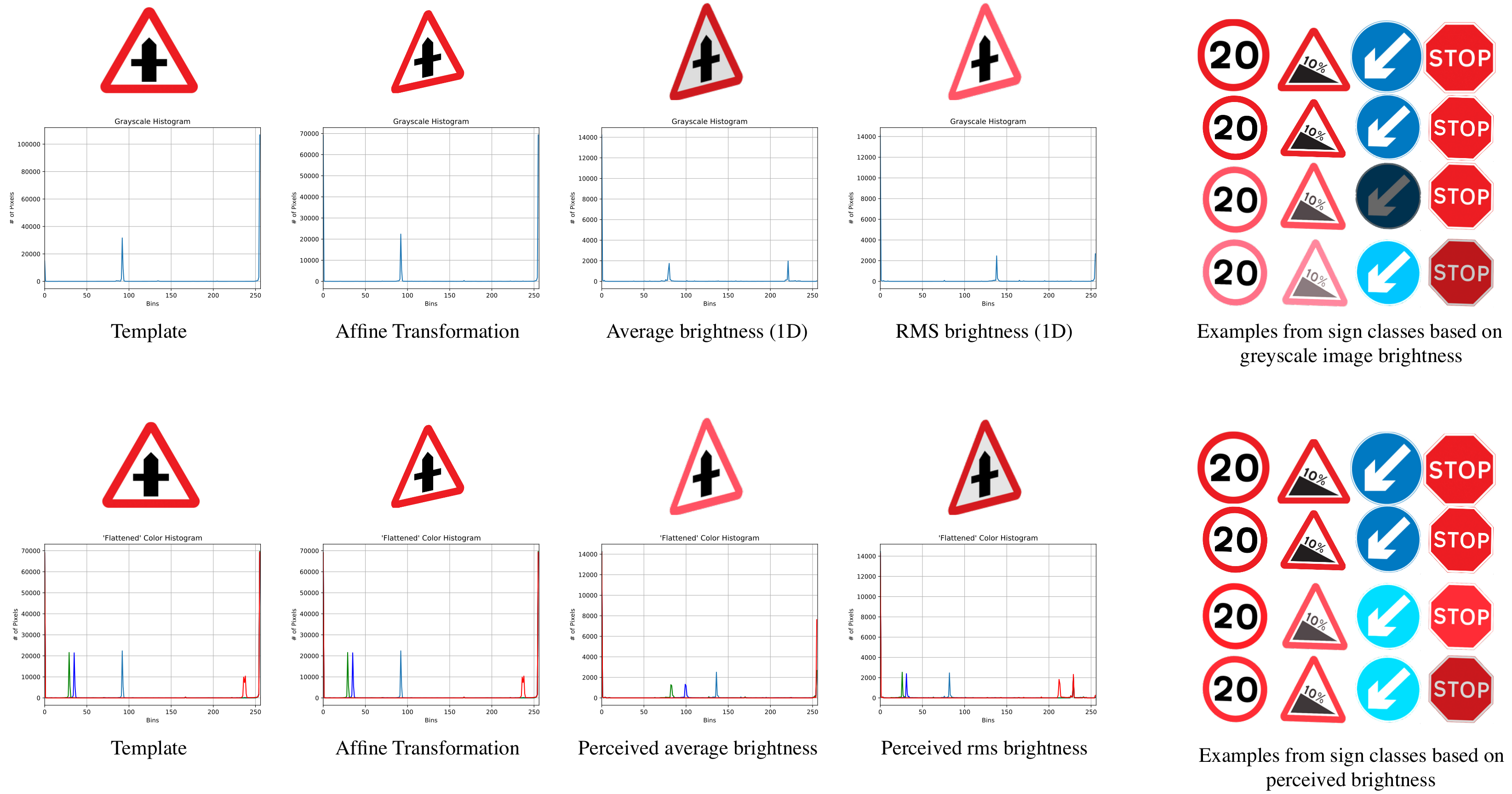
3.3. Dataset Normalisation

The main part that the normalisation process is responsible for is applying a non-local means denoising that produces a blurred version of the image, by replacing the colour of each pixel with an average of similarly-coloured pixels. This filter has proven to provide better results than the standard Gaussian filter, as it allows the effective denoising of the actual data in the validation set, as well as tempering with the appearance of the synthetic data in order to minimise the features that do not exist in real examples. Furthermore, by considering all the similar pixels in a region and assigning the average value, the colour similarity between the training and validation set increases significantly. Although the classifier is only concerned with a single dimension, the variations conducted in all of three channels of the images will also be represented in the grey-scaled version of the images, as well. The kernel used to apply the filter is five by five in size in order to accomplish a box blur without introducing a large enough distortion that would alter the visual features of the sign. The similarity of the synthetic examples compared to real images can be seen in Figure 4.

4. Classification Scheme

The main methodology that is used for classification and testing the dataset generation pipeline is a convolutional neural network. The intuition behind using this model is its robustness towards viewpoint, pose and appearance variations.

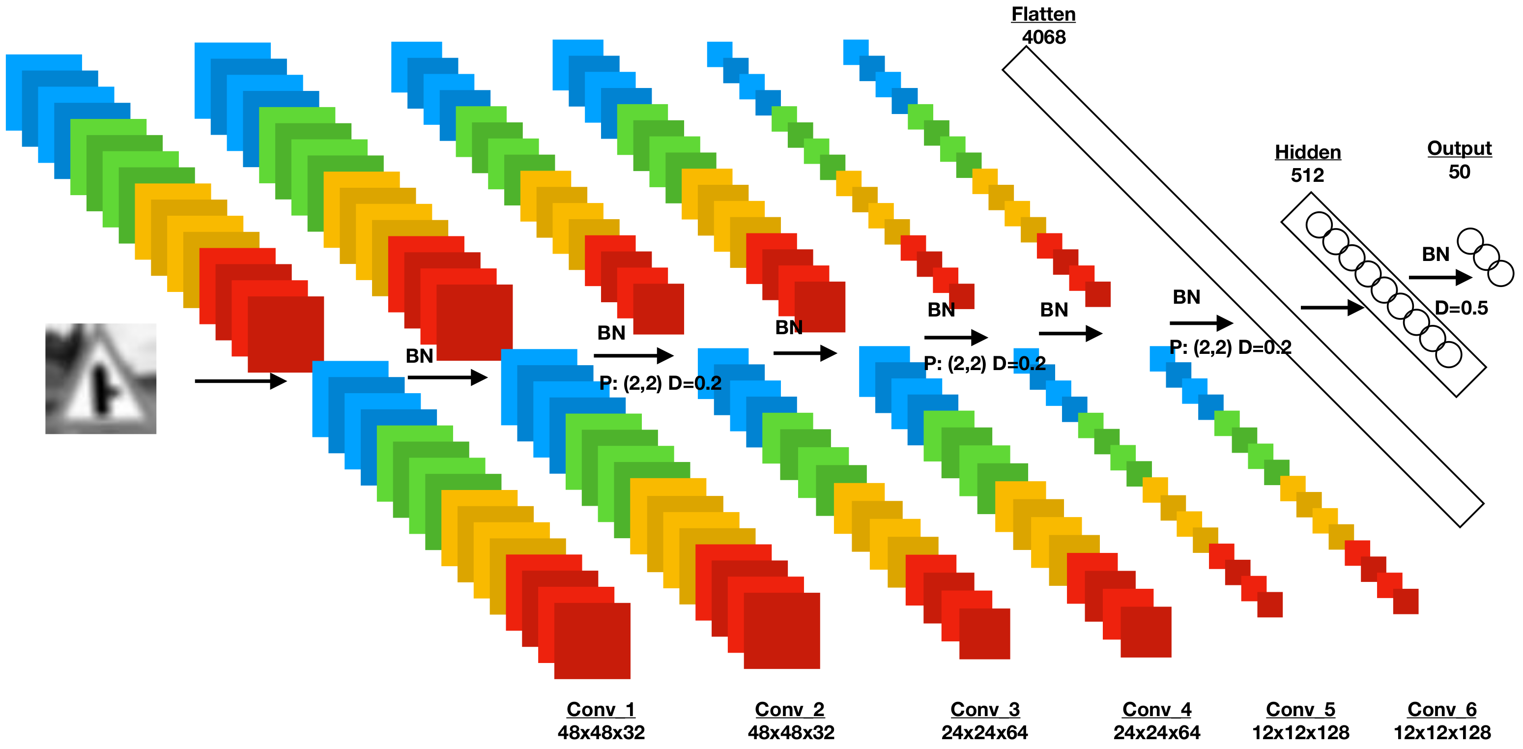
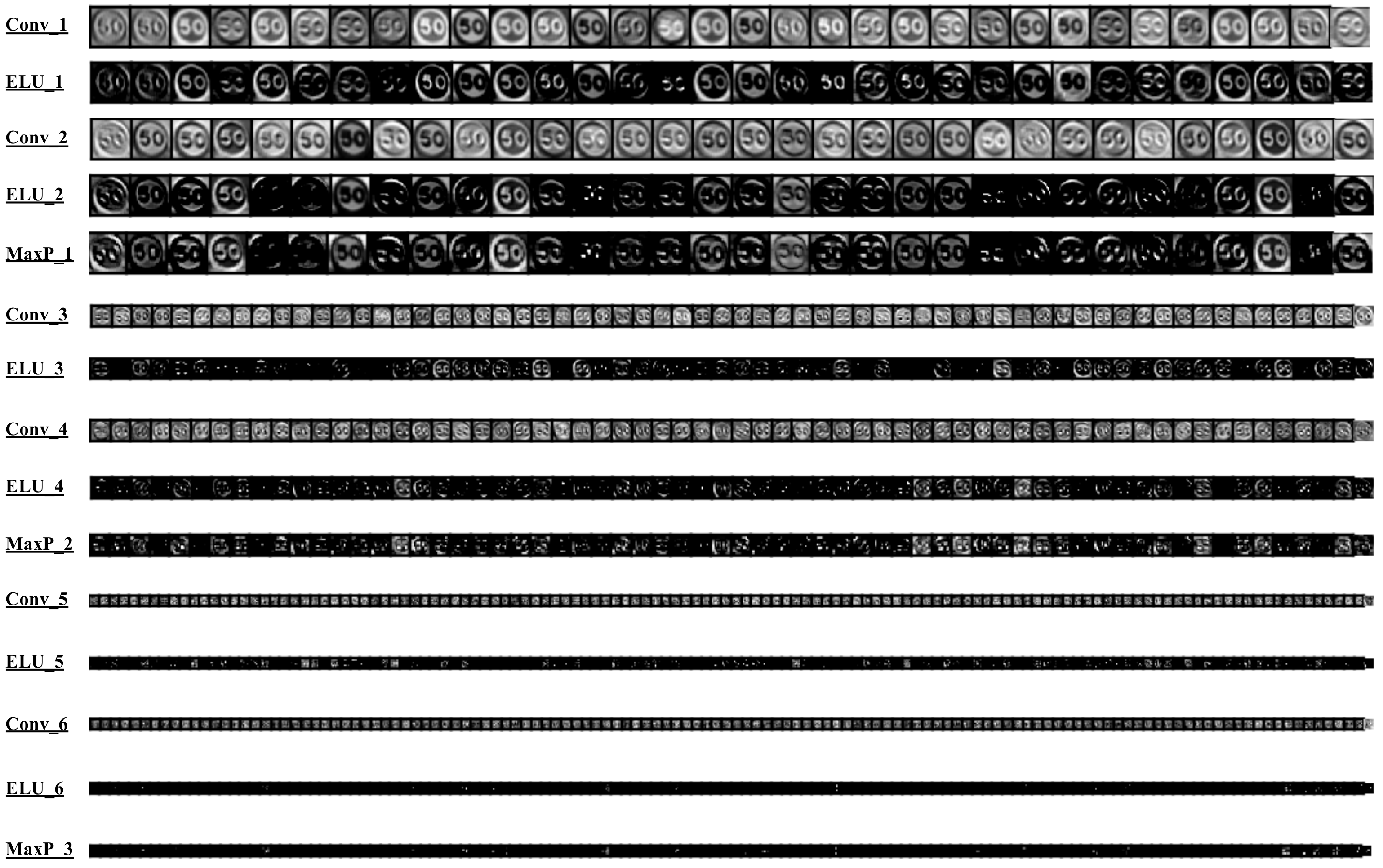
4.1. CNNs and Three-Dimensional Image Depth

One of the main advantages of CNNs in image recognition tasks is the fact that they are capable of holding all three dimensions of an image (width, height and depth/colour) within their neurons, as shown by Sermanet and LeCun [3]. CNNs are feed-forward models, which means that information moves only in one direction, similarly to our visual cortex, where cortical neurons (regions of the mammalian brain) are responsible for specific regions and what is perceived in the field of vision. Conceiving an entire environment is achieved by overlapping those fields. Each neuron in succeeded layers is only connected to a small region of the previous layer, and the network is learning the underlying features directly from data (training examples provided).

The architecture of our proposed network is depicted in Figure 5. It consists of six convolutional layers responsible for learning a hierarchical representation of the underlying features in input images, with max poolingand dropout layers used every two convolutional layers and a hidden layer that maps the outputs of the flattened layer, consisting of the one-dimensional matrix of the images, to their respected classes in the output layer. Exponential Linear Unit (ELU) [24] activation functions are applied to the output of every convolutional and dense layer alongside batch normalisation, with the exception of the last layer, which is responsible for outputting class predictions, in which a Softmax activation was applied. The kernel sizes used in all convolution layers are 3 × 3. The number of output layer neurons can be changed in order to accommodate traffic sign templates with different sizes from the image generation process.

4.2. Utilising Exponential Linear Units

The need for a more advanced activation layer derives from the shortcomings of the standard Rectified Linear Units (ReLU) activation function, which has proven to be very sensitive during training. More specifically, when the model optimiser, in combination with the learning rate, forces a large weight update during that step, this will cause the neuron to not activate on the new data sample. This problem is known as `dying ReLU’ and has been an inspiration for the introduction of different activation functions over the last few years. When this problem occurs, the gradient of the neuron will `freeze’ to a zero value from that point onwards during the classifier’s training.

The ReLU rectifier is fast to compute since the function simply outputs zero for smaller-than-zero input and essentially mimics the identity function. In any other case, the derivative will be equal to one. More formally, it is summarised in Equation (6).

$$\frac{d}{d_x}{f}_{\left(x\right)}=\left\{\begin{array}{c}0ifx<0\hfill \\ 1ifx>0\hfill \end{array}\right.,Notdifferentiableatx=0$$

(6)

For this reason, ReLU cannot recover from this issue as not only the output will be zero, but also the derivative will have a zero value. Although this pitfall has been the cause for research, one of its advantages is the sparsity of the representations that is fed to it during training. An example of this can be perceived through information disentangling, as in a highly dense representation, major changes in the input would resolve to large modifications in the representation vector appearance. Alternatively, including small, robust and sparse delineations preserves the feature throughout iterations [25]. Additionally, sparse representations are more probable to be linearly separable since the multi-dimensional space of the examples can also effectively reflect the original data. Furthermore, considering the fact that different inputs may hold a different information size, than previous ones, using a shifting-size structure to obtain information may yield better results. By changing the number of active neurons at each step, the dimensionality of the model can be controlled and tailored according to the data. However, dense representations are shown to produce a greater amount of information, as they are exponentially richer than the selective sparse counterpart.

For the needs of our model, rectified linear units were not used as the difference between the training and validation samples was large enough to an extent to which, a sparse representation would not include examples with features that are better distinguishable than what would have been seen in a dense structure. This is due to the synthetic nature of the training data and, thus, the need for a higher complexity system with a greater number of parameters that would have a constant architecture.

The need for a different rectifier unit led to testing four other alternatives to ReLU. The one that showed the best rates and consistency on the validation set loss was the Exponential Linear Unit (ELU). Essentially, the choice for ELU was mainly due to the fact that both leaky ReLUs and parametrised ReLUs also include negative values and do not ensure effective reduction of image noise. The advantage of ELUs is the analysis of the percentage of a phenomenon in the input, while the lack of that phenomenon is not mapped quantitatively. This also provides a generalisation method for the entire network, which is deemed necessary in the case of synthetic training data. Equation (7) describes the activation function with the alpha value used.

$$f_{\left(x\right)}=\left\{\begin{array}{c}\alpha \times (e^x-1)forx<0\hfill \\ xforx\ge 0\hfill \end{array}\right.,f_{\left(x\right)}^{\prime }=\left\{\begin{array}{c}1forx<0\hfill \\ f_{\left(x\right)}+\alpha forx\ge 0\hfill \end{array}\right.,where\alpha =0.001$$

(7)

As it is observed, by including a constant, ELU can saturate based on that value, when the inputs are negative. This also allows for the activation to adequately deal with the vanishing gradient problem. The main contrast from the other rectifiers is that ELUs takes negative values that push the gradient closer to zero. This also provides a clear distinction for the activation in terms of the instances in which it is active and inactive. ELUs can also limit the gap between the unit gradient and the normal gradient, improving the training time rate. This feature is also the key component of batch normalization, which will be discussed in Section 4.3. This constrainment that is introduced with this function allows the rectifier to outperform the previously suggested methods in tests that were done in a variety of different task (such as optical character recognition with the MNISTdataset, as well as the use of a 15-layer CNN on the ImageNet) [26]. For this dataset, ELUs are found to be singly slower than other activations, mainly due to the hyperbolic function that has been utilised for negative values, instead of the linear equation found in LReLuand PReLu. However, the influence of the activation function is considered to be minimal during training, especially when the number of iterations is extensive and the volume of data is substantial [27].

4.3. Normalisation

A considerable limitation of large-scale neural networks is the fact that each layer’s inputs are modified during every training iteration, as the parameters of the previous layer that the current layer is connected to change. The outcome of this is slower rates during training and produces difficult to train models with non-linearities. This problem is known as the internal covariance shift and perceived as the variation in the activations of the model, in terms of their distribution, because of the continuous change of parameters during each training step. A way to solve the internal covariance shift problem is the use of a normalisation technique for each layer’s input as introduced in Ioffe and Szegedy [28]. The essence of this method is that normalisation becomes an integral part of the entire model and thus performed on each batch of data as passed to the model, at every epoch during the training phase. This also implies faster training, since the stability of non-linearly-separable cases of inputs becomes stronger and the optimiser avoids remaining in the saturated condition. The gradient flow of the entire network can also be improved by this technique, since the dependence of gradients in parameters that are shifted at each epoch or to their initial values are significantly reduced. Additionally, the improvement minimises the risk of divergence for the deep network, without a compensation for the learning rate of the system. This also provides the means for a smoother dropout [29] as randomising the outputs of one layer becomes less important, due to the fact that normalisation is performed first. The initial technique used for batch normalisation [28] was based on modifications of the inputs at each layer to achieve a constant distribution of features. This modification can be perceived as either creating a dependency on the activation values for the optimiser or a direct change in the overall network structure [30,31].

Because the task at hand includes cases of non-differentiable types of inputs, the normalisation function has the format seen in Equation (8).

$$({x\prime }^{\left(n\right)})=\frac{x^{\left(n\right)}-E\left[x^{\left(n\right)}\right]}{\sqrt[]{Variance\left[x^{\left(n\right)}\right]}},where:E[x^{\left(n\right)}]=\frac{1}{N}\times \sum _{i=1}^N{x}_i^{\left(n\right)}$$

(8)

As is observed from the equation, the normalisation is equal to the result produced by subtracting from the n-dimensional space layer input ($x=(x^{\left(1\right)},x^{\left(2\right)},\dots ,x^{\left(n\right)})$) the mean of all the values used in training, with their respected dimensionality, divided by the square root of the unbiased variance estimate ($Variance\left[x^{\left(n\right)}\right]=\frac{m}{m-1}$). A greater than one mini-batch size (m) is used for this operation. This also avoids the decorrelation of the image features through layers of the network. However, normalising each input individually may cause variations to what the network perceives. This can also gradually decrease the accuracy, and thus, caution is necessary when normalisation is performed. If the identity transform can be effectively represented by the transformation inserted in the network, the normalisation has been applied effectively. In a neural network that includes batch normalisation and has been trained with it, each example in the training procedure is used concurrently with other examples of the batch. This allows the network to avoid deterministic values that are solely based on single instances for each example. For the requirements of our system, batch normalisation has been applied to every convolution layer (Layers 2–6), and additionally, the outputs of the last convolution layer, before the data are compressed to a single-dimension vector of which its elements correspond to the features extracted by the previous convolutional layers, as seen in Figure 5. With the proposed network, the total number of parameters associated with normalisation was pushed to 3840. It is clear that the batch normalisation method that was utilised shows many similarities to a proposed standardisation layer [32]. Batch normalisation targets stable distributions during each pass of the mini-batch through the network, while the normalisation layer is applied non-linearly to the output of the previous layer to achieve sparse activations.

4.4. Sample-Based Discretisation

The hierarchical image features extracted by the convolutional layers are used for the classification process. Utilising the feature space has proven to be computationally challenging as if the dimensionality of the images through the network remains the same, and the total number of parameters increases. What is required is a method that can progressively reduce the overall complexity of inputs of convolutional layers by minimising the spatial size of the feature maps. These layers are commonly referred to as `Pooling Layers’ in which the input representations are down-sampled. The process of pooling includes the use of aggregate statistics in specific parts of the image, which include distinct features. This normally is performed by using the mean or max value of an image to represent the feature with a decreased dimensionality. The pooling layer can be added to any part of the network as it acts independently on every depth slice of the image and resizes it appropriately. One of the most common pooling techniques is the utilisation of the maximum or mean value present in a region selected by the defined kernel. Thus, the required variables in order to construct a pooling layer are the following:

• The size of the filter to be used. Most filters in max pooling are either of size 2 × 2 or 3 × 3, as based on these values, the kernel will traverse the entire image matrix. Furthermore, taking into account the use of the mean or max value at each traverse, the system will compute and output the suitable value.
• The stride of the kernel, as it defines the step that is used while passing through the image vector. A larger stride will resolve in a smaller output, since less pixels will overlap between kernel steps. For example, a 2 × 2 filter with a stride of two will resolve in non-overlapping pixels in the final output down-scaled feature vector.

In this work, between every two convolution layers, a max-pooling layer was added for decreasing the image dimensionality, as it has shown that it works better in practice than mean or average pooling. The kernel size was set to 2 × 2 with a stride of two, for each pooling operation, and therefore, the output will have half the width and half the height of the original image. The layer outputs can be visualised in Figure 6.

4.5. Regularisation

Due to the large number of parameters, as well as the the complexity of the method, our main concern is overfitting. For this reason, the well-known dropout technique is utilised for addressing this problem. This technique is closely related to the natural theory of evolution and the reproduction system that exists in nature and is perceived as a stochastic regularisation method. However, it can be managed in order to acquire deterministic regulisers. Dropout stochastically reduces the loss function by applying a noise distribution procedure.

Consider a neural network with H hidden layers, where we use h for an index $h\in$ {1, 2, …, H} and the two vectors for inputs and outputs are defined as $i{n}^{\left(h\right)}$ and $ou{t}^{\left(h\right)}$. The weight of the layer is $W^{\left(l\right)}$, the bias $b^{\left(l\right)}$ and the feed forward operation with dropout defined in Equation (9) for every hidden unit i, where $r^{\left(l\right)}$ is the vector of Bernoulli random variables, with probability p being one and is used in conjunction with $i{n}^{\left(h\right)}$ to create the thinned inputs by the dropout function ${\widetilde{out}}^{\left(h\right)}$.

$$\begin{array}{c}\hfill i{n}_i^{(h+1)}=W_i^{(h+1)}\times {\widetilde{out}}^{\left(h\right)}+b_i^{(h+1)}ou{t}_i^{(h+1)}=activation\left(i{n}_i^{(h+1)}\right)\\ \hfill where{\widetilde{out}}^{\left(h\right)}=r^{\left(h\right)}\times i{n}^{\left(h\right)}and{r}^{\left(h\right)}\sim Bernoulli\left(p\right)\end{array}$$

(9)

Dropout can be utilised in neural networks with the use of gradient decent, with the exception that each batch of training examples is passed to a `thinned’ version of the network, since some units were not used. Both forward and back propagation are done to the thinned version of the network. The gradients of each parameter are averaged over the course of the training steps, with parameters that do not contribute to the network (since they have been dropped) taking a gradient value of zero.

In our network, dropout was used four times, three of which were between the convolutional layers in which the depth of the image is modified and just before the images are flattened, while the last dropout was utilised before the output layer of the network. The dropout at the convolutional layers of the network is kept at 20%. The difference in the hidden layer and the dropout that is applied to its output is that 0.5 probability, showing the maximum amount of regularisation [33], as it is the most important layer, since it is responsible for determining the class of the image passed in the network. Furthermore, a 50% rate would yield an equal distribution for every network that is produced through each training step.

5. Experimental Results

5.1. Implementation Details

Experiments performed with the use of generated data from training were produced based on fifty different classes and applied twenty distinct affine transformations. The final set was constructed from 1000 background images and four different brightness variations. The total number of generated images was 2 M, while their distribution across categories in the dataset was not uniform. For this reason, the experiments were performed on samples from each of the categories that reinsure stratification of classes between the training and validation sets. The classifier was fed with 3400 images for each class, and the total number of training images was 170,000. The validation was performed on 2500 real-world images. Because of the magnitude of the SGTSD that was created, sampling based on human intuition was not possible to be performed within the given time-frame; therefore, the sample chosen for each sign was composed of randomly selected images. The accuracy rates achieved and presented were based on the average values that the network converged to once no further improvement was shown by the network.

The batch size of the network was 32. The creation of this mini-batch and its use for training were to limit the training time required by the network. This was based on the trade-off between the batch size and the number of iterations used to train the network. An increase in the batch size may also show a decrease in the ability of the model to generalise (which is one of the most important aspects of this work, as the difference between real and synthetic sets were greater than in other similar systems) [34]. This is because of the tendency of large batches to become sharp minimisers when training. Thus, sharp minima consequently led to poorer generalisation, when on the other hand, small batches converged to flat minimisers since there was an inherited noise in the gradient estimation process. This was also shown when taking the loss function, as large batches were heavily engaged in regions where a sharp minima existed, while on the contrary, small batches were bound to small positive eigenvalues.

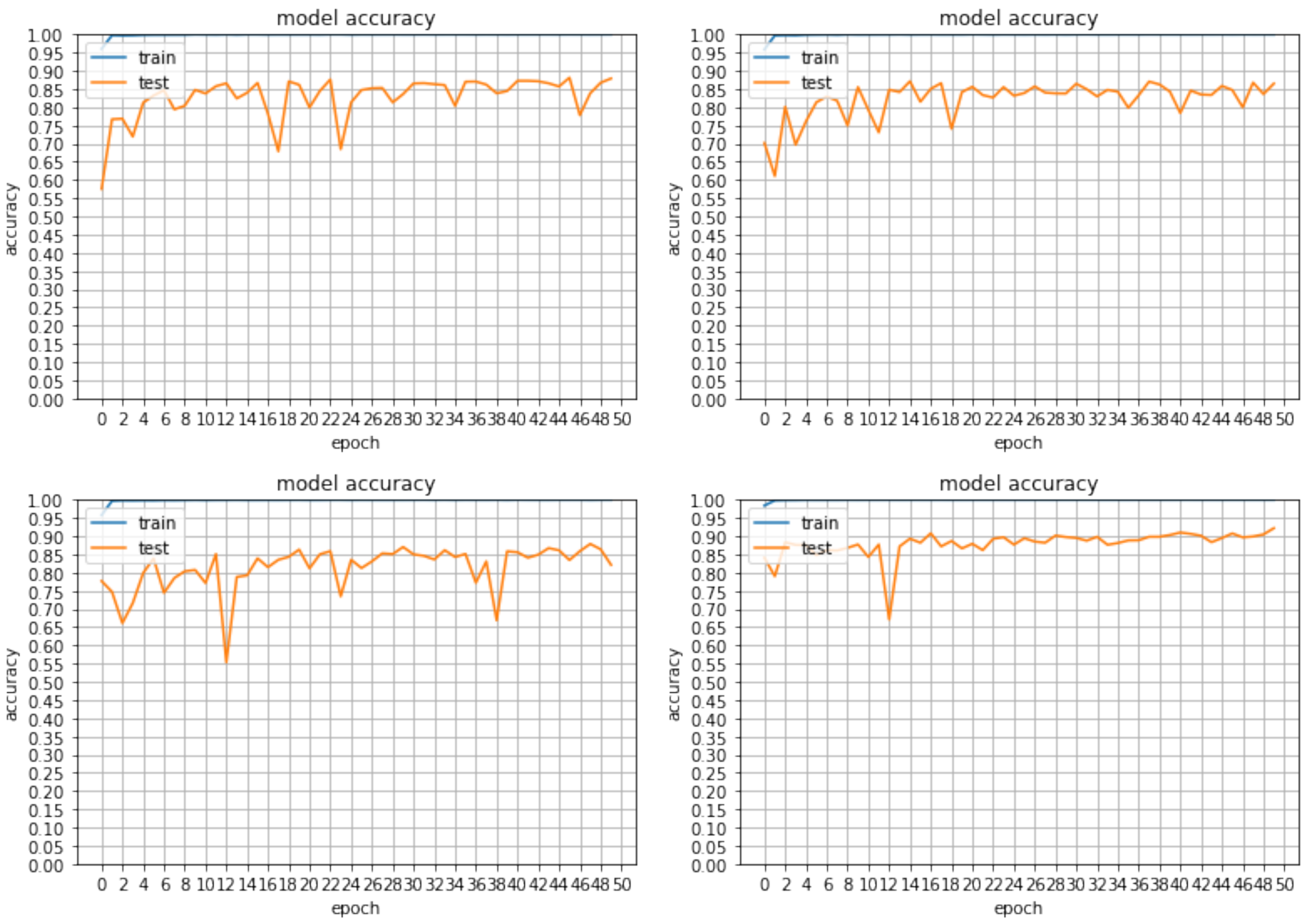
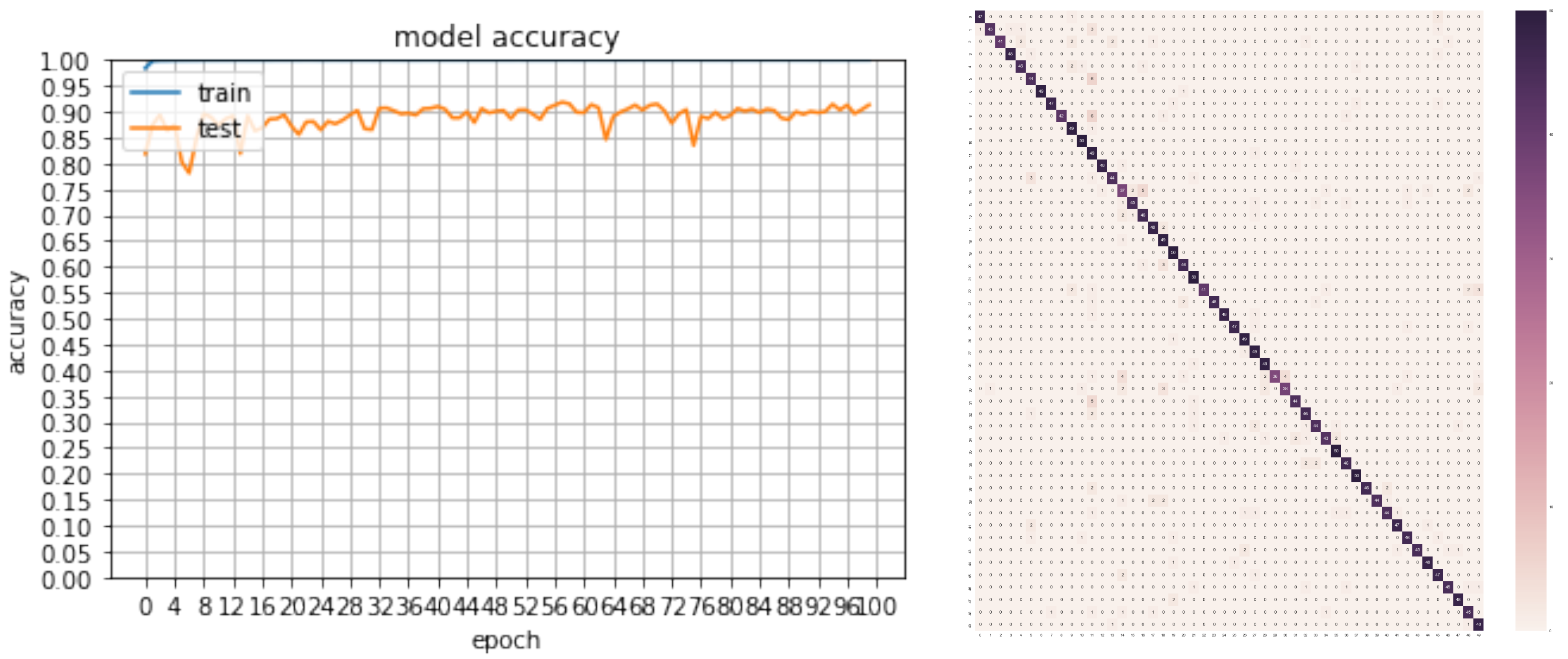
5.2. Classification Results

The best accuracy achieved by our baseline classifier was 91.84% after 100 epochs of training. It was shown that by applying Batch Normalisation (BN), the model was able to generalise significantly better since the accuracy was boosted from 87.88%, which was outputted from a previous network version, and with the use of ELU as a rectifier, it reached 92.20%, with the same sample and number of epochs. Although initially, as is seen in

Table 2. Accuracy and Kappa statistic rate achieved using synthesised training data for different models with their respective number of iterations. ELU, Exponential Linear Unit.

Classifier Type	Accuracy Rates (%)	Kappa Statistic
CNN w/Leaky ReLU—0 epochs	87.88%	0.8788
CNN w/ PReLu, 50 epochs	87.03%	0.8703
CNN w/ ELU—50 epochs	87.88%	0.8788
CNN w/ ELU and BN, 50 epochs	92.20%	0.9219
CNN w/ ELU and BN, 100 epochs, new data	91.84%	0.9183

and Figure 7, using leaky ReLu and PReLu, the accuracy rates were higher during a larger number of iterations than the ones achieved with ELU, the loss function remained very high for these two rectifiers (close to 1.5, while ELU showed a decrease with 1.0). Although the two activation functions were not efficiently tested on the new classifier, ELU showed great improvement when approximating the identity of an example in cases that were close to the origin because of its exponential nature, while both PReLu and leaky ReLu cannot. Although the difference in rectifiers showed little difference in the runs performed, a more notable increase was shown with BN, as non-trainable parameters allowed the construction of a better model that could map the difference of real data as used for validation and synthetic data for training.

Remarkably, the quantitative results of Table 2 show that the model was capable of performing close to the lower and mid-nineties accuracy when the full system was utilised.

Although the margin between the created system and others that are a part of the current state-of-the art and utilise real data for training was high, the outcomes are promising, as they showed that with the correct sampling (difference between the two last runs), the margin could be minimised even more. In terms of the error cases, as can be seen by the truth table in Figure 8, the classes that displayed lower true positive results by the model were the two classes (28 and 29) that were similar, as they both were warning signs associated with the narrowness of the road ahead (“narrow road on the right lane” and “narrow road on the left lane”, respectively).

Based on the rates achieved and the alternative state-of-the art methods, we can make several conclusions. We have shown that our synthesised training data can be used for training a robust classifier, which learned effectively most of the descriptive features. Although a margin of up to 7.8% existed between the state-of-the art recognition models and our method, remarkably, our system was able to generalise the features that were learned over other examples beyond the specified training dataset utilising a significantly less complex architecture compared to alternatives. Taking more training data with a larger variance of the utilised illumination conditions and the utilised viewpoints led to an increasing performance. This clearly demonstrates the power of using synthesised traffic signs for practical applications.

6. Conclusions and Future Work

In this paper, we have presented an approach for creating synthetic training samples for traffic sign recognition. In this way, it is possible to eliminate the need for a predefined set of training examples tailor-made for one country. In addition, using synthesised data overcomes the need for time-consuming manual acquisition, annotation and segmentation of images. To evaluate our approach, we acquired a database of traffic signs, containing 50 classes and a total number of 2 M images, from which the training data were generated. Using this dataset and a simple end-to-end image classification scheme, we built a data-driven traffic sign recognition system that can achieve close to state-of-the-art results, as well as high computational efficiency. Our evaluation demonstrates that our approach represents a significant step towards recognising traffic signs using exclusively synthesised training images.

Further advancements can be targeted towards texture synthesis to represent the materials of the traffic signs more effectively. One possible issue regarding this approach might be the fact that road signs are considered as “glossy” materials due to the fact that the incoming light of a given direction (which might be from the sun or street lighting) is not reflected equally on the material and not in one direction, as well. This also means that the directions to which the light is reflected to may change when the optical perspective of the observer has changed. However, the sign will have a reflective nature in the case where the light is coming from a car’s headlights, as they are designed to be specular in that specific light hue. Therefore, a deep understanding of the sign material needs to be established by the system in order to be able to compute the different outcomes that can be expected for applying light of different sources and angles at the sign.

References

- Fu, M.Y.; Huang, Y.S. A survey of traffic sign recognition. In Proceedings of the IEEE International Conference on Wavelet Analysis and Pattern Recognition (ICWAPR), Qingdao, China, 11–14 July 2010; pp. 119–124. [Google Scholar]
- Miura, J.; Kanda, T.; Nakatani, S.; Shirai, Y. An active vision system for on-line traffic sign recognition. IEICE Trans. Inf. Syst. 2002, 85, 1784–1792. [Google Scholar]
- Sermanet, P.; LeCun, Y. Traffic sign recognition with multi-scale convolutional networks. In Proceedings of the 2011 IEEE International Joint Conference on Neural Networks (IJCNN), San Jose, CA, USA, 31 July–5 August 2011; pp. 2809–2813. [Google Scholar]
- Stallkamp, J.; Schlipsing, M.; Salmen, J.; Igel, C. The German traffic sign recognition benchmark: A multi-class classification competition. In Proceedings of the 2011 IEEE International Joint Conference on Neural Networks (IJCNN), San Jose, CA, USA, 31 July–5 August 2011; pp. 1453–1460. [Google Scholar]
- Bascón, S.M.; Rodríguez, J.A.; Arroyo, S.L.; Caballero, A.F.; López-Ferreras, F. An optimization on pictogram identification for the road-sign recognition task using SVMs. Comput. Vis. Image Underst. 2010, 114, 373–383. [Google Scholar] [CrossRef]
- Larsson, F.; Felsberg, M. Using Fourier descriptors and spatial models for traffic sign recognition. In Proceedings of the Scandinavian Conference on Image Analysis, Ystad, Sweden, 23–27 May 2011; pp. 238–249. [Google Scholar]
- Timofte, R.; Zimmermann, K.; Van Gool, L. Multi-view traffic sign detection, recognition, and 3D localisation. Mach. Vis. Appl. 2014, 25, 633–647. [Google Scholar] [CrossRef]
- Akatsuka, H.; Imai, S. Road Signposts Recognition System. SAE Trans. 1987, 96, 936–943. [Google Scholar]
- de Saint Blancard, M. Road sign recognition. In Vision-Based Vehicle Guidance; Springer: Berlin, Germany, 1992; pp. 162–172. [Google Scholar]
- Zaklouta, F.; Stanciulescu, B. Real-time traffic sign recognition in three stages. Robot. Auton. Syst. 2014, 62, 16–24. [Google Scholar] [CrossRef]
- Yao, C.; Wu, F.; Chen, H.J.; Hao, X.L.; Shen, Y. Traffic sign recognition using HOG-SVM and grid search. In Proceedings of the IEEE 2014 12th International Conference on Signal Processing (ICSP), Hangzhou, China, 19–23 October 2014; pp. 962–965. [Google Scholar]
- Cireşan, D.; Meier, U.; Masci, J.; Schmidhuber, J. Multi-column deep neural network for traffic sign classification. Neural Netw. 2012, 32, 333–338. [Google Scholar] [CrossRef] [PubMed]
- Scherer, D.; Müller, A.; Behnke, S. Evaluation of pooling operations in convolutional architectures for object recognition. In Proceedings of the International Conference on Artificial Neural Networks, Thessaloniki, Greece, 15–18 September 2010; pp. 92–101. [Google Scholar]
- Ueda, N. Optimal linear combination of neural networks for improving classification performance. IEEE Trans. Pattern Anal. Mach. Intell. 2000, 22, 207–215. [Google Scholar] [CrossRef]
- Meier, U.; Ciresan, D.C.; Gambardella, L.M.; Schmidhuber, J. Better digit recognition with a committee of simple neural nets. In Proceedings of the IEEE 2011 International Conference on Document Analysis and Recognition (ICDAR), Beijing, China, 18–21 September 2011; pp. 1250–1254. [Google Scholar]
- Haloi, M. Traffic Sign Classification Using Deep Inception Based Convolutional Networks. arXiv 2015, arXiv:1511.02992. [Google Scholar]
- Jin, J.; Fu, K.; Zhang, C. Traffic sign recognition with hinge loss trained convolutional neural networks. IEEE Trans. Intell. Transp. Syst. 2014, 15, 1991–2000. [Google Scholar] [CrossRef]
- Szegedy, C.; Liu, W.; Jia, Y.; Sermanet, P.; Reed, S.; Anguelov, D.; Erhan, D.; Vanhoucke, V.; Rabinovich, A. Going Deeper with Convolutions. In Proceedings of the 2015 IEEE Conference on Computer Vision and Pattern Recognition (CVPR), Boston, MA, USA, 7–12 June 2015. [Google Scholar]
- Traffic Sign Images. Available online: https://www.gov.uk/guidance/traffic-sign-images (accessed on 17 January 2018).
- Berger, M. Geometry I; Springer: Berlin, Germany, 2009. [Google Scholar]
- Jain, A.K. Fundamentals of Digital Image Processing; Prentice Hall: Englewood Cliffs, NJ, USA, 1989. [Google Scholar]
- Connolly, T.G.; Sluckin, W. Introduction to Statistics for the Social Sciences; Springer: Berlin, Germany, 1971. [Google Scholar]
- Finley, D. HSP Color Model— Alternative to HSV (HSB) and HSL. 2006. Available online: http://alienryderflex.com/hsp.html (accessed on 26 July 2018).
- Clevert, D.A.; Unterthiner, T.; Hochreiter, S. Fast and Accurate Deep Network Learning by Exponential Linear Units (Elus). arXiv 2015, arXiv:1511.07289. [Google Scholar]
- Bengio, Y. Learning deep architectures for AI. Found. Trends Mach. Learn. 2009, 2, 1–127. [Google Scholar] [CrossRef]
- He, K.; Zhang, X.; Ren, S.; Sun, J. Delving deep into rectifiers: Surpassing human-level performance on imagenet classification. In Proceedings of the IEEE International Conference on Computer Vision, Santiago, Chile, 13–16 December 2015; pp. 1026–1034. [Google Scholar]
- Jia, Y. Learning Semantic Image Representations at a Large Scale; University of California: Berkeley, CA, USA, 2014. [Google Scholar]
- Ioffe, S.; Szegedy, C. Batch normalization: Accelerating deep network training by reducing internal covariate shift. arXiv 2015, arXiv:1502.03167. [Google Scholar]
- Srivastava, N.; Hinton, G.; Krizhevsky, A.; Sutskever, I.; Salakhutdinov, R. Dropout: A simple way to prevent neural networks from overfitting. J. Mach. Learn. Res. 2014, 15, 1929–1958. [Google Scholar]
- Povey, D.; Zhang, X.; Khudanpur, S. Parallel training of Deep Neural Networks with Natural Gradient and Parameter Averaging. arXiv 2014, arXiv:1410.7455. [Google Scholar]
- Wiesler, S.; Richard, A.; Schluter, R.; Ney, H. Mean-normalized stochastic gradient for large-scale deep learning. In Proceedings of the 2014 IEEE International Conference on Acoustics, Speech and Signal Processing (ICASSP), Florence, Italy, 4–9 May 2014; pp. 180–184. [Google Scholar]
- Gülçehre, Ç.; Bengio, Y. Knowledge matters: Importance of prior information for optimization. J. Mach. Learn. Res. 2016, 17, 226–257. [Google Scholar]
- Baldi, P.; Sadowski, P.J. Understanding Dropout. In Advances in Neural Information Processing Systems 26; Burges, C.J.C., Bottou, L., Welling, M., Ghahramani, Z., Weinberger, K.Q., Eds.; Curran Associates, Inc.: Red Hook, NY, USA, 2013; pp. 2814–2822. [Google Scholar]
- Nitish, S.K.; Dheevatsa, M.; Jorge, N.; Mikhail, S.; Tang, P.T.P. On Large-Batch Training for Deep Learning: Generalization Gap and Sharp Minima. arXiv 2016, arXiv:1609.04836. [Google Scholar]
Sample Availability: A sample of the code and results obtain can be found in: https://github.com/
alexandrosstergiou/Traffic-Sign-Recognition-basd-on-Synthesised-Training-Data. |