Subject-Specific BCI Frameworks for Motor Imagery Classification Based on BSS-Free and BSS-Equipped Pipelines

Abstract

The development of Motor Imagery (MI) Brain–Computer Interfaces (BCIs) is systematically constrained by low signal-to-noise ratios (SNRs), signal non-stationarity, and acute data scarcity. While complex Blind Source Separation (BSS) methods optimize signal clarity, their computational overhead introduces propagation delays that challenge real-time constraints. This study addresses this engineering trade-off by introducing a localized architectural framework to evaluate whether a lightweight pipeline operating without BSS (No-BSS) is sufficiently efficient for real-time control when compared against two BSS-equipped pipelines utilizing Independent Component Analysis (ICA) and Empirical Mode Decomposition (EMD). Validated across the BCI Competition IV Dataset 2A and the PhysioNet MI dataset, all three pipelines share an identical processing chain designed to maximize efficiency. To mitigate low SNRs, an Adaptive Laplacian spatial filter isolates neural intent across target sensorimotor electrodes (C3, C4, and Cz). Data scarcity is countered via a Gaussian noise injection data augmentation strategy, while session-to-session variability is addressed during feature extraction using Wavelet Packet Decomposition (WPD) paired with a Fisher Score criterion to dynamically isolate subject-specific time-frequency nodes. Redundant features are subsequently eliminated using a Genetic Algorithm (GA) before classification. Experimental evaluation reveals a distinct performance stratification: while the ICA (92.80%) and EMD (92.69%) pipelines yield the highest average accuracy for the PhysioNet dataset by isolating non-stationary and physiological noise, the No-BSS baseline (90.28%) remains the superior framework for the BCI Dataset 2A. Across all pipelines across both datasets, a stable classification hierarchy emerges wherein the Support Vector Machine (SVM) leads performance due to its maximum-margin decision boundary, followed by k-Nearest Neighbors (kNN), a modified EEGNet, and Decision Trees. The No-BSS baseline achieves classification accuracies highly competitive with its BSS counterparts while entirely bypassing their algorithmic overhead. Given the strict latency constraints of live BCI control loops, these findings establish the optimized No-BSS pipeline as a highly viable alternative for low-latency, real-time implementations.

1. Introduction

BCI technology establishes a direct communication pathway between neural activity and external applications, such as robotic prosthetics or motorized wheelchairs [1,2,3]. These systems function by decoding MI, the imagination of a physical action performed without actual muscular contraction. By capturing these endogenous brain signals, individuals can generate digital control commands through cognitive intent alone. Electroencephalography (EEG) remains the preferred modality for recording these intentions due to its non-invasive nature, portability, and superior temporal resolution [4]. The raw EEG signal consists of rhythmic electrical oscillations categorized into distinct frequency bands that correspond to specific physiological and cognitive states. These waveforms, ranging from Delta and Theta to Alpha, Beta, and Gamma, typically follow an inverse relationship between frequency and power. Higher-frequency oscillations such as Alpha and Beta, which are important for detecting motor imagery, exhibit significantly smaller amplitudes than the slower, high-voltage waves such as Delta or Theta [5]. This disparity in signal strength underscores the primary challenge in BCI design: isolating subtle motor-related perturbations from dominant background activity.

The detection of MI depends on monitoring specific sensorimotor rhythms, primarily localized within the Alpha and Beta frequency bands. When an individual imagines moving a limb, a characteristic decrease in spectral power occurs within these frequencies, a phenomenon termed Event-Related Desynchronization (ERD). A subsequent increase in power is observed, known as Event-Related Synchronization (ERS), once the mental task is completed. The precise identification of these amplitude shifts serves as the fundamental mechanism for converting mental intent into digital control commands [5,6].

The presence of physiological and non-physiological artifacts frequently degrades EEG recordings, leading to a decrease in the Signal-to-Noise Ratio (SNR). Unlike the rhythmic nature of actual brain activity, these disturbances are typically transient and characterized by higher amplitudes. There are three primary categories of interference that impact these recording sessions: environmental factors, experimental errors, and systemic physiological processes [7,8,9]. Each of these manifests through distinct physical properties that alter the integrity of the measured signal. Environmental noise often manifests as a 50/60 Hz hum from nearby power leads or electromagnetic interference from external radiation. In these instances, the measurement cables or the human body itself can act as an antenna, picking up radio frequency (RF) or magnetic disturbances [7,8,9]. Fortunately, because these signals usually occupy a narrow frequency band outside the range of functional brain activity, they can often be eliminated using standard filtering techniques. However, experimental errors present a different challenge; simple subject movements can shift the physical contact of an electrode on the scalp. This change in placement alters the electrical coupling and volume conduction between the neural source and the sensor, leading to voltage fluctuations that severely distort the output [7,8,9].

The most difficult interference to manage comes from physiological processes. Eye movements and blinks are particularly disruptive because the shifting resting potential of the retina creates an Electrooculogram (EOG) signal. Due to the proximity of the eyes to the brain, these high-amplitude signals spread across the scalp and can overwhelm the subtle neural intent being recorded. Similarly, muscle tension, especially in the face or jaw, creates Electromyogram (EMG) artifacts that span a broad frequency range, while cardiac activity can introduce rhythmic pulse artifacts as blood vessels expand and contract near the sensors. Understanding these specific spectral properties is important for designing the filters and optimization algorithms required for a reliable BCI system [7,8,9].

Another obstacle in developing reliable BCI systems is the inconsistent accuracy of MI predictions, driven by session-to-session variations in EEG characteristics. The difficulty in maintaining high performance stems from the inherently non-linear and non-stationary nature of neural signals [10,11,12]. In a non-stationary time series, statistical properties such as the mean and variance are not constant; instead, it fluctuates over time due to the existence of trends or seasonality. These shifts in the distribution of EEG features over time often lead to discrepancies between training and testing datasets. Within even a single recording session, these changes in feature patterns can impair a classifier’s ability to generalize, ultimately reducing the accuracy of EEG-based BCI systems.

Furthermore, the non-linearity of EEG signals indicates that the electrical activity of the brain does not follow a simple, predictable pattern where outputs are directly proportional to inputs [12]. Because of this complexity, small changes in a subject’s mental state can trigger significant or unexpected fluctuations in the recorded signal. This intricate behaviour makes it difficult for conventional linear techniques to effectively process and classify neural intent. As a result, these non-linear complexities often result in reduced system performance, highlighting the challenges of using standard methods to navigate the patterns found in scalp EEG. This necessitates the development of a modular framework that can autonomously optimize feature selection to maintain classification stability.

The implementation of Blind Source Separation (BSS) methods in MI-BCIs introduces a severe compromise between classification accuracy and computational demand [2,13]. Traditional artifact rejection techniques such as ICA and EMD utilize iterative sifting loops and heavy matrix calculations that perform well in offline simulations. However, this processing overhead scales poorly in real-time environments, creating execution latencies that violate the tight temporal windows necessary for closed-loop control. As a result, developing a localized and BSS-free pipeline is critical to achieving competitive decoding accuracies without the processing lag.

The primary contributions of this research are summarized as follows:

• Low-Latency BCI Framework: Formulated a BSS-free pipeline that removes the need for computationally expensive decomposition (ICA/EMD) without sacrificing accuracy, specifically optimized for real-time applications.
• Integrated Artifact Suppression: Developed a dual-layer strategy combining Adaptive Laplacian Spatial Filtering with statistical trial pruning to eliminate volume conduction and high-amplitude noise while maintaining a minimal computational footprint.
• Adaptive Manifold Optimization: Resolved subject-specific variance and BCI illiteracy by implementing an adaptive WPD framework that dynamically aligns signal frequency sub-bands, further optimized by a GA for high-precision feature selection.
• Robust Data Augmentation: Implemented a stochastic Gaussian noise injection strategy that introduces non-repeating signal variations across epochs, mitigating data scarcity and enhancing model generalizability against temporal non-stationarity.
• Cross-Architecture Stability Benchmarking: Validated the framework’s robustness against temporal non-stationarity by benchmarking it across diverse models (SVM, KNN, Decision Tree, EEGNet) for evaluating BCI signal processing reliability.

These contributions provide a unified framework that improves upon standard, isolated feature-based approaches. By integrating these preprocessing and classification steps, this research demonstrates how to optimize a pipeline, balancing the trade-off between computational efficiency and classification accuracy in asynchronous BCI systems.

The remainder of this paper is organized as follows: Section 2 reviews the relevant literature regarding MI limitations. Section 3 details the mathematical framework of the processing pipelines, including the spatial filtering, BSS configurations, feature extraction and classification stages. Section 4 presents the experimental results and evaluates performance across the different pipelines and models. Section 5 discusses the real-time engineering trade-offs, analyzes methodological and clinical limitations, and Section 6 concludes the paper by outlining key findings and future work.

2. Related Work

2.1. Engineering Trade-Offs in MI-BCI Design

The broader engineering motivation for efficient physiological-signal classification centers on the critical balance between model complexity, predictive performance, and deployment feasibility. The recent literature in resource-aware biomedical artificial intelligence has shifted toward identifying classification strategies that remain functional within the strict temporal and energy constraints of portable medical hardware. Reference [14] demonstrated this principle by implementing a common spatial pattern and Riemannian manifold-based SVM pipeline on embedded systems, achieving only 0.08 to 0.3 s of computation time and approximately 15 MB of memory usage on Raspberry Pi and Jetson Nano. While high-performance architectures such as deep convolutional networks offer superior accuracy, their heavy processing overhead can create execution latencies that hinder real-time deployment in daily life monitoring scenarios. Reference [15] highlighted this tension by demonstrating that relatively simple EEG preprocessing pipelines, when carefully calibrated, can achieve reliable MI decoding without the parameter-heavy architectures increasingly adopted in the field. To address these limitations, recent research emphasizes streamlined pipelines such as automated channel selection and feature fusion strategies that prioritize computational efficiency without significant loss of reliability. Reference [16] illustrated this approach by combining functional connectivity features with translation-invariant scattering coefficients through a multiclass SVM classifier, outperforming single-feature baselines on the BCI Competition IV-2a dataset while maintaining a computationally tractable pipeline. Reference [17] further demonstrated that multivariate empirical mode decomposition combined with discrete wavelet transform and SVM classification yields interpretable results with a reduced variable set, avoiding the overfitting risks associated with deeper architectures. Furthermore, addressing the trade-off between algorithmic sophistication and practical usability is essential for overcoming the illiteracy phenomenon in neural control systems, ensuring that biomedical AI remains accessible even in resource-limited or high-variability environments. Reference [18] addressed this challenge through a two-stage refine filtering method that improves signal quality in BCI systems, enhancing classification reliability for users who struggle with standard MI protocols. This focus on efficiency-driven design ensures that physiological signal processing remains robust across diverse clinical and real-world applications while maintaining the speed necessary for closed-loop diagnostic systems.

2.2. Overview of Data Augmentation

Data augmentation has become an essential strategy for addressing data scarcity in EEG-based motor imagery BCI systems, where deep learning performance is often constrained by subject fatigue and signal drift. Reference [19] introduced an empirical mode decomposition (EMD)-based approach to generate synthetic frames by mixing intrinsic mode functions (IMFs) from real trials, achieving up to 88.2% accuracy on BCI competition datasets. However, this method faces technical hurdles: EMD lacks a rigorous theoretical foundation and is prone to end effects and mode-mixing [20]. Furthermore, reference [19] noted that their Wavelet Neural Network (WNN) model occasionally failed to converge when trained on larger sets of these artificial frames and exhibited high standard deviation in accuracy, suggesting that synthesized data may introduce instabilities. Similarly, reference [21] proposed an amplitude-perturbation method using short-time Fourier transform (STFT), but as [22] argue, such noise injection must be approached with caution. Blindly adding Gaussian noise using fixed statistical properties is often ineffective due to the non-stationary nature of EEG signals. Instead, reference [22] recommend a zero-mean noise tailored to the specific trial’s mean amplitude to preserve underlying neural patterns. While ref. [22] systematically compared six techniques to move beyond naive computer vision adaptations, they acknowledge that many current augmentation studies remain restricted by their reliance on single datasets, which limits the generalizability of their results across different populations and EEG paradigms. To address these limitations, this study implements a stochastic Gaussian noise injection strategy that builds upon the recommendations of [22] by tailoring noise to trial-specific characteristics. By advancing this methodology through the introduction of non-repeating, stochastic fluctuations across training epochs, the framework moves beyond the constraints of static variation.

2.3. Multi-Resolution Analysis: DWT vs. WPD

Time-frequency decomposition using wavelets, particularly the Discrete Wavelet Transform (DWT) and Wavelet Packet Decomposition (WPD), serves as a fundamental approach for feature extraction in MI-BCI research. The DWT operates by recursively partitioning EEG signals into approximation (low-frequency) and detail (high-frequency) coefficients; however, because it typically decomposes only the approximation components, its spectral resolution is inherently restricted [23]. WPD addresses this limitation by decomposing both coefficient types at every stage, resulting in a comprehensive binary tree structure where each node captures a more refined frequency band. Reference [24] illustrated the efficacy of this approach by utilizing a six-level WPD to identify 27 distinct nodes within the 8–32 Hz range, highlighting nodes (6,10) and (6,11) as particularly responsive to MI.

Despite these benefits, WPD presents notable disadvantages. The exhaustive nature of the full binary tree structure imposes a significant computational burden, as each level of decomposition doubles the number of filtering and downsampling operations required. Additionally, the resulting high-dimensional feature sets often lead to data redundancy and an increased susceptibility to overfitting, which necessitates the inclusion of secondary feature selection processes that vary in reliability. Furthermore, the selection of an optimal mother wavelet remains an unresolved issue, as performance is highly dependent on specific signal characteristics rather than a universal standard [24]. Reference [20] emphasized that determining the ideal number of decomposition levels poses a further challenge, as this choice directly impacts the balance between spectral precision and computational overhead. Finally, reference [25] demonstrated that DWT’s hierarchical decomposition structure, though computationally lightweight, yields coarser spectral representations compared to WPD’s full binary tree decomposition. Consequently, these studies demonstrate that while WPD offers superior informational richness compared to DWT, the tension between spectral resolution and computational demand remains a primary design consideration for real-time BCI architectures.

2.4. Overview of Feature Selection

In EEG-based MI systems, feature selection is a vital process for mitigating the curse of dimensionality and ensuring classifier efficiency, particularly when handling high-dimensional, multiband signal data. Research by [26] highlighted that while Genetic Algorithms (GA) are effective for identifying optimal subsets via evolutionary pressure, the Relief-F algorithm consistently achieves superior performance, reaching 91.43% accuracy on BCI Competition III Dataset IVA and demonstrating higher robustness against the noise inherent in non-stationary EEG signals.

A primary distinction in this domain lies between wrapper and filter-based approaches: wrapper methods, such as GA, excel at capturing complex synergistic effects between features by evaluating subset interactions, whereas filter-based methods often overlook these dependencies by treating features in isolation. Despite the power of wrapper methods, reference [26] noted that FBCSP-based architectures often struggle with high-dimensional input and are highly sensitive to signal quality. Similarly, reference [4] demonstrated the use of Neighborhood Component Analysis (NCA) to optimize CSP features with 81.52% average accuracy, yet this approach provided no guarantee of identifying a globally optimal feature subset.

Furthermore, the integration of bio-inspired heuristics including Ant Colony, Firefly, and Artificial Bee Colony optimization has introduced sophisticated alternative strategies for automated channel ranking and feature selection in high-dimensional spaces [20]. Collectively, these findings underscore that while feature selection is essential for BCI performance, no universal methodology exists. Instead, the efficacy of any chosen technique remains intrinsically linked to dataset characteristics, the quality of the EEG signals, and the requirements of the specific classification task.

3. Material and Methods

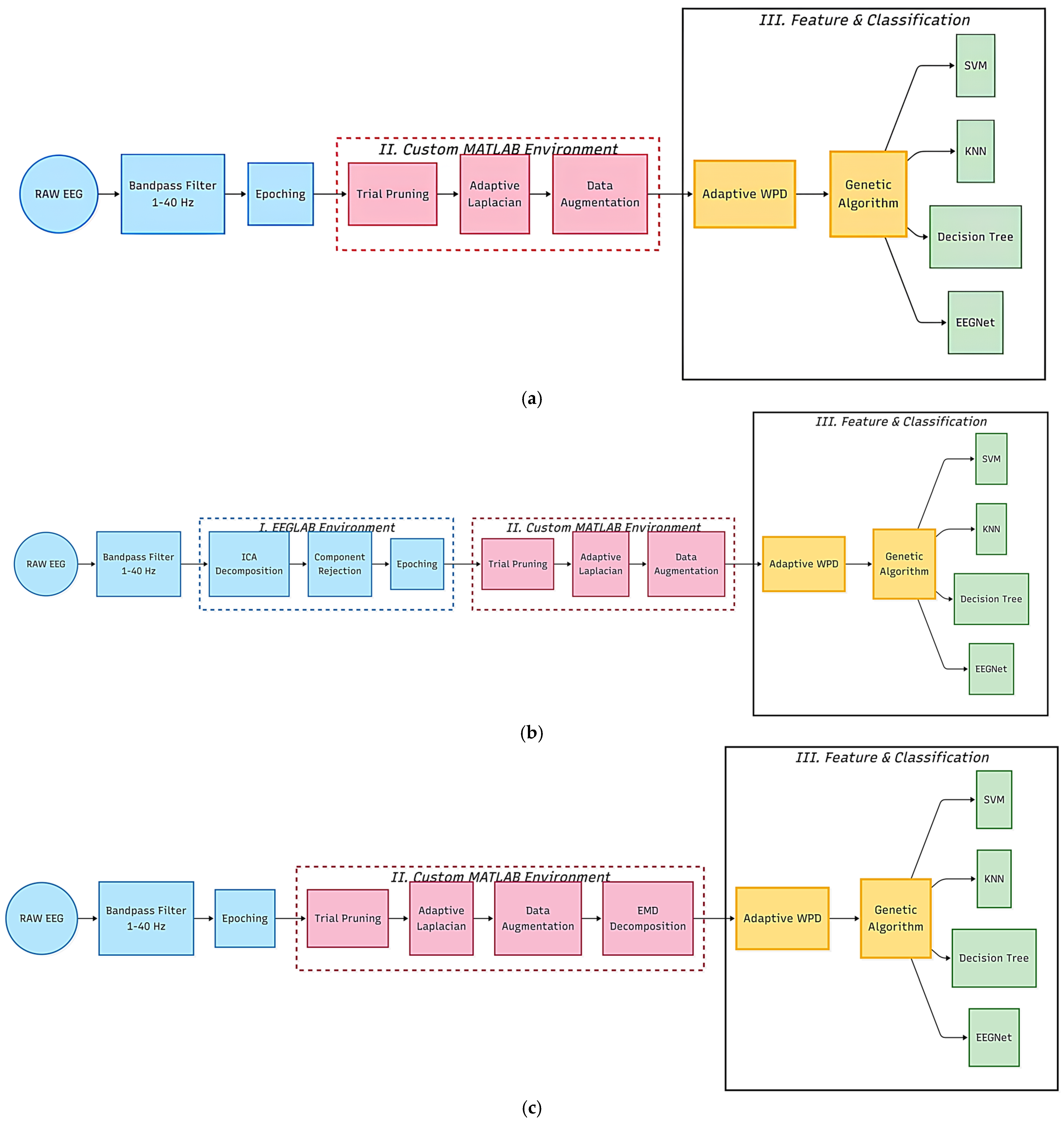
This study utilizes a comparative methodological framework to assess how three different pipelines manage poor SNR and session-to-session variations during MI classification. Throughout the flowcharts in Figure 1, the blue blocks represent the processes executed within the EEGLAB user interface, while the pink blocks designate the operations handled in the custom MATLAB environment. The No-BSS baseline, presented in Figure 1a, establishes a performance boundary by completely omitting BSS. In contrast, the ICA pipeline shown in Figure 1b uses ICA within EEGLAB to separate and eliminate physiological artifacts. In this pipeline, the Adaptive Laplacian filter is positioned to ensure it acts upon the reconstructed signal. The EMD pipeline shown in Figure 1c applies EMD to extract data-driven, non-linear Intrinsic Mode Functions (IMFs) matching the natural oscillatory patterns of the brain. Within this specific topology, EMD is intentionally positioned after data augmentation so that the iterative sifting optimizes directly on the unified properties of the newly synthesized trials. For pipeline uniformity, all three pipelines merge into a standardized backend that has the Adaptive Laplacian filter configured to mitigate volume conduction and enhance localized Mu and Beta rhythm signal directly at the motor cortex. An Adaptive Wavelet Packet Decomposition (WPD) to isolate distinct neural patterns in discriminative nodes. A GA handles global feature selection before routing the optimized feature vectors into four classifiers: Decision Tree, KNN, ECOC-SVM, and a modified EEGNet, thereby maintaining stable decision boundaries against non-stationary shifts in the underlying EEG data distribution.

3.1. Data Acquisition

The framework was evaluated using two benchmark datasets: the BCI Competition IV (Dataset 2a) and the PhysioNet EEG Motor Imagery Dataset. These provide a robust baseline for testing the pipelines against both high-resolution (250 Hz) and lower-resolution (160 Hz) MI signals.

3.1.1. BCI Competition IV Dataset 2A

EEG signals were recorded at 250 Hz using a 22-channel Ag/AgCl monopolar configuration with a 3.5 cm inter-electrode distance. The recording was referenced to the left mastoid with the right mastoid serving as ground. Initial signal conditioning included a 0.5–100 Hz band-pass filter and a 50 Hz notch filter at 100 µV sensitivity. Additionally, three monopolar EOG channels were recorded at 1 mV sensitivity to facilitate ocular artifact rejection during the preprocessing stage, ensuring these non-neural signals were excluded from the final movement classification. The dataset includes nine subjects performing four motor imagery tasks: left hand, right hand, both feet, and tongue. Each subject participated in two sessions of 288 trials each, totaling 576 trials. Prior to recording, a five-minute EOG calibration was conducted covering eyes open, eyes closed, and active eye movements to provide a baseline for ocular artifact rejection [27].

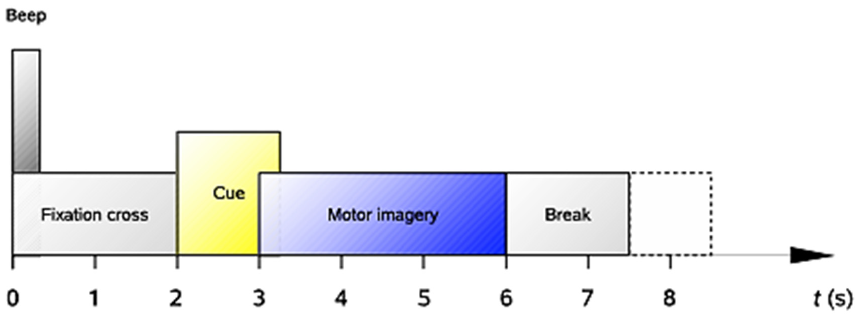
Subjects were seated in a comfortable armchair facing a computer monitor to perform the task. Each individual trial followed the temporal sequence illustrated in Figure 2 [27]:

• t = 0 s: A fixation cross appeared on a black screen accompanied by an acoustic tone to signal the trial’s onset.
• t = 2 s: A directional arrow (left, right, down, or up) appeared for 1.25 s to cue the specific motor imagery task.
• t = 2 s to 6 s: Subjects performed the cued task without feedback until the fixation cross was removed at t = 6 s.
• Post-trial: A brief rest period with a black screen occurred before the next trial sequence began.

3.1.2. PhysioNet EEG Motor Imagery Dataset

The PhysioNet Dataset is a repository of 1500 EEG recordings from 109 volunteers. To ensure an unbiased evaluation, this study utilizes a cohort of 9 volunteers (S001–S009) selected randomly from the total dataset prior to analysis. This selection was made without prior knowledge of individual performance or signal quality, intentionally avoiding selection bias. As a result, the results serve as a proof-of-concept validation of the framework’s robustness within a diverse subset, rather than a comprehensive evaluation of the entire PhysioNet population. Data were recorded through the BCI2000 system using a 64-channel International 10-10 montage, with specific peripheral electrodes (Nz, F9, F10, A1, A2) excluded to prioritize cortical areas relevant to motor imagery. The experimental protocol consisted of 14 sequential runs per subject, including two one-minute baseline sessions (eyes open/closed) and twelve two-minute motor task runs. These runs covered unilateral (left vs. right fist) and bilateral (both fists vs. both feet) coordination. The dataset uses a tripartite annotation system (T0, T1, T2): T0 denotes a rest state, while T1 and T2 mark the onset of imagery or motion for the respective cued tasks [28].

To overcome the dataset’s shifting annotation system and ensure sufficient data for training, the following preprocessing steps were implemented:

• Event Synchronization: Since the meaning of the markers T1 and T2 depends on the specific run index, a manual re-mapping was implemented in EEGLAB. In runs involving the hands (Runs 4, 8, 12), markers were mapped to T1 (Left Hand) and T2 (Right Hand). In runs involving bilateral coordination (Runs 6, 10, 14), these were mapped to T3 (Both Hands) and T4 (Both Feet), resulting in a consistent 4-class framework.
• Multi-Run Concatenation: All task-relevant runs for each subject were merged into a single continuous EEG structure. This was performed prior to artifact rejection to provide the ICA algorithm with a statistically robust signal length, ensuring more accurate decomposition of non-neural sources.

3.2. Signal Processing

Signal processing was conducted in the EEGLAB environment in MATLAB r2017b, utilizing a four-stage pipeline to enhance the SNR and ensure data consistency.

3.2.1. Digital Filtering

To isolate the Mu (8–12 Hz) and Beta (12–30 Hz) rhythms [29], a 1–40 Hz FIR filter was applied to the signal. The filter’s order (N) was determined by the toolbox’s default heuristic described in Equation (1):

$$N=3\left({\displaystyle \frac{f_s}{locutoff}}\right)$$

(1)

where $f_s$ is the sampling frequency and locutoff is the low cut off frequency.

This resulted in a filter order of 105 for the 250 Hz dataset and 66 for the 160 Hz dataset. This stage acted as the primary noise-rejection layer by removing low-frequency ocular drifts and high-frequency muscle interference. Implementing the filter before advanced artifact rejection is important. It stabilized the signal and improved data retention by preventing the subsequent algorithms from over-correcting for baseline noise.

3.2.2. Epoching

Epoching is a critical preprocessing stage where continuous EEG signals are segmented into time-locked windows to isolate task-specific neural activity [30]. In this study, the continuous data were epoched according to the specific timing paradigms of each respective dataset. The signal was segmented into 3.5-s epochs for the BCI Competition Dataset 2A and 4.5 s epochs for the PhysioNet dataset, relative to the onset of the MI cues (left hand, right hand, foot, tongue, both fists, both feet). Following the epoching procedure, the EEGLAB remove baseline function was applied to the epochs. This step utilized the 500 ms pre-stimulus interval (−0.5 to 0 s) as a reference to calculate and subtract the mean value from each trial [15].

3.2.3. Trial Pruning

A statistical trial pruning procedure was used to prevent extreme artifacts from distorting classifier training [31]. For each trial, the temporal variance was calculated across all EEG channels and summed to create an aggregate variance metric. Trials with a total variance exceeding a dynamic threshold of 2.5 standard deviations above the session mean were flagged as heavily contaminated by high-amplitude noise, such as muscle movements or electrode shifts. These noisy trials were removed to ensure only clean data reached the feature selection and classification stages.

3.3. Blind Source Separation (BSS) Comparison

3.3.1. Independent Component Analysis

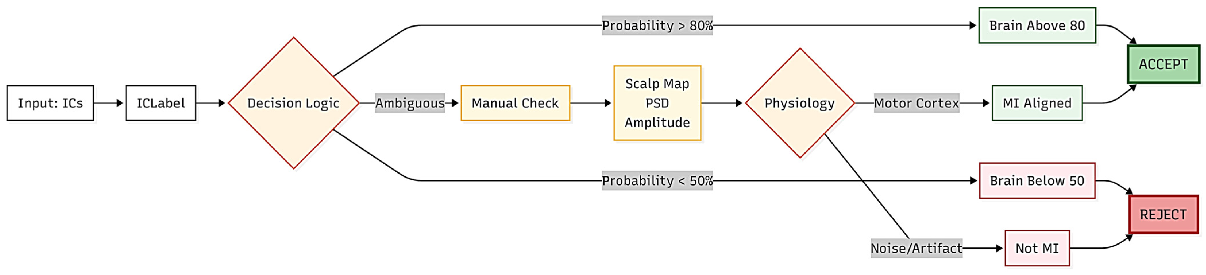
Independent Component Analysis (ICA) was implemented through the RUNICA algorithm within the EEGLAB environment to decompose multivariate EEG signals into statistically independent, non-Gaussian sources. This process is essential for unmixing neural signatures from physiological artifacts, such as eye blinks and muscle tension [6,32,33]. To ensure the integrity of the MI features, the extracted Independent Components (ICs) were subjected to a rigorous dual-validation process combining ICLabel automated classification with manual visual inspection of topographical scalp maps. To minimize subjectivity, this inspection was conducted according to a strict, pre-defined protocol, as shown in Figure 3:

• Automated Filtering: Components were automatically accepted if the Brain class probability exceeded 80% and combined noise (Muscle, Eye, Heart) remained below 20%. In contrast, components were rejected if Brain probability fell below 50% or combined noise exceeded 20%.
• Structured Manual Protocol: Ambiguous components (where probabilities fell between 50 and 80%) were subjected to an objective assessment based on three criteria:
  • Spatial Distribution: Components were rejected if the scalp map displayed localized, non-cortical activity such as ocular or temporal artifacts rather than the bilateral distribution expected during MI.
  • Spectral Profiling: Components were rejected if the Power Spectral Density (PSD) exhibited non-physiological characteristics, such as high-frequency wide-band noise from muscle tension, or excessive low-frequency power, from blink artifacts.
  • Temporal Stability: Components were cross-referenced with time-series amplitude to identify transient, non-stationary artifacts.

This approach ensured that manual interventions were based on objective neurophysiological markers, maintaining consistency and reproducibility across all subjects.

3.3.2. Fast Empirical Mode Decomposition

The signal decomposition is executed on an epoch-by-epoch basis through a Fast EMD implementation tailored to isolate IMFs from non-stationary EEG signals [25,34]. To improve reproducibility, the sifting process was capped by a fixed stopping threshold of two iterations to limit residual-error propagation and avoid algorithmic divergence [34]. This granular approach ensures that the decomposition remains localized to the MI task window, preventing temporal leakage from non-task-related brain activity. While standard EMD typically relies on cubic spline interpolation, pipeline B utilizes Piecewise Cubic Hermite Interpolating Polynomials (PCHIP) to define the sifting process envelopes. Choosing PCHIP over traditional cubic splines improves the mathematical rigor and stability of the BCI system, specifically targeting challenges such as SNR and session-to-session variability through a shape-preserving, third-degree Piecewise Polynomial Function (PPF) [35]. Compared to cubic splines, this method matches only first-order derivatives at data points, ensures the interpolant’s minimum aligns with the data’s minimum, and maintains monotonicity wherever the underlying data is monotonic. As a result, PCHIP produces significantly less overshoot and undershoot than cubic splines, resulting in a more stable mean envelope for identifying MI signatures [35,36].

The decomposition procedure initiates by formatting the input signal into a column vector to maintain uniformity in matrix calculations throughout the process. This is represented by the following framework:

• Decomposition Model and IMF Constraints

• To focus on the most significant neural signatures, such as Mu and Beta rhythms, the algorithm is constrained to isolate a maximum of three IMFs. The original signal x(t) is modelled as defined in Equation (2):

  $$x(t)={\displaystyle {\sum }_{i=1}^k}{IMF}_i\left(t\right)+r_k\left(t\right) where k \le 3$$

  (2)

  Restricting the output to three IMFs isolates relevant neural oscillations from background baseline drifts. This ensures a stable feature space and minimizes frequency leakage, resulting in a more robust and consistent decomposition [37].

2.

Boundary Constraints and PCHIP Interpolation

• Throughout the execution, the system identifies local maxima ${(p}_i)$ and minima ${(v}_i)$ to build the upper ${(e}_{up})$ and lower ${(e}_{lo})$ signal boundaries. By including the initial and final signal samples as boundary constraints, the PCHIP interpolation maintains its mathematical integrity and avoids edge divergence as shown in Equation (3):

  $$e\left(1\right)=x\left(1\right) and e\left(n\right)=x\left(n\right)$$

  (3)

  Choosing PCHIP over traditional cubic splines ensures the interpolation is shape preserving and prevents overshoot.

  $$e_{up}\left(t\right)=P_{pchip}\left(p_i, t\right), e_{lo}\left(t\right)=P_{pchip}\left(v_i, t\right)$$

  (4)

3.

Mean Envelope Extraction

• As a result, the mean of these envelopes is removed from the signal to extract a distinct neural component, with the leftover residue serving as the input for subsequent extraction phases. The local mean m(t) is calculated as Equation (5):

  $$\begin{gathered} m\left(t\right)= {\displaystyle \frac{e_{up}\left(t\right)+ e_{lo}(t)}{2}} \\ {IMF}_{new}\left(t\right)= {IMF}_{old}\left(t\right)-m\left(t\right) \end{gathered}$$

  (5)

3.4. Spatial Enhancement and Optimization

3.4.1. Adaptive Laplacian Spatial Filter

The methodology utilizes an Adaptive Laplacian Spatial Filter to counteract the spatial distortion caused by volume conduction, a process where the skull’s resistive properties cause electrical currents to spread laterally and smear across the scalp [38]. This operation acts as a spatial high-pass filter, reversing the blurring effect that typically leads to coherence inflation and poor source discrimination by removing broad, overlapping voltage patterns to uncover the focal cortical activity beneath [39]. The choice of an Adaptive Laplacian filter over a fixed one is driven by the need to handle the dynamic, unpredictable nature of EEG signals and variations in volume conduction across subjects. The adaptive spatial filtering process is governed by the following four-stage mathematical framework, executed on an epoch-by-epoch basis.

• Spatial Correlation Weighting

• While traditional fixed filters use rigid, pre-set coefficients based solely on where the electrodes are placed, the adaptive approach constantly recalibrates its weights based on the statistical relationship between the target electrode and its neighbors. For a target electrode $x_j$, the raw spatial weights $w_i$ for each neighbour $n_i\in N_j$ are determined by the Pearson Correlation coefficient. A threshold of 0.3 is applied to ensure only spatially redundant noise is considered:

  $$w_i= \left\{\begin{array}{c}corr\left(x_j, x_i\right) if corr\left(x_j, x_i\right)>0.3\\ 0 otherwise\end{array}\right.$$

  (6)

  This threshold is designed to mitigate the smearing effect while ensuring that subtle, task-specific MI patterns remain preserved. By filtering only those electrode pairings with a correlation above 0.3, redundant spatial noise is effectively suppressed without losing the fine-grained information essential for high-accuracy MI classification. This flexibility is important for managing the session-to-session variability and low SNR typical of motor imagery tasks, as it allows the pipeline to adjust to the specific brain activity of each subject.

2.

Weight Normalization

• The spatial weights are normalized to unity ($\sum {\widehat{w}}_i=1)$ as shown in Equation (7), ensuring the resulting noise estimate is proportional to the target channel’s local field potential. This normalization prevents artificial amplitude distortion and guarantees that the conservatism factor remains scaled consistently, regardless of subject-specific or session-to-session signal variance.

  $${\widehat{w}}_i={\displaystyle \frac{w_i}{{\sum }_{k\in N_j}{w}_k}}$$

  (7)

3.

Weighted Spatial Noise Estimation

• The smeared noise L(t) is constructed by calculating the weighted sum, as shown in Equation (8), of the neighboring channels identified in Table 1:

  $$L\left(t\right)= {\sum }_{i \in N_j}{\widehat{w}}_i \times x_i\left(t\right)$$

  (8)

Table 1. Electrode index layout for the localized Adaptive Laplacian spatial filter.

Target Electrodes	BCI Competition IV 2A Neighbors	PhysioNet Neighbors
C3	2, 7, 9, 14	2, 16, 8, 10
Cz	4, 9, 11, 16	4, 18, 10, 12
C4	6, 11, 13, 18	6, 20, 12, 14

Table 1. Electrode index layout for the localized Adaptive Laplacian spatial filter.

Target Electrodes	BCI Competition IV 2A Neighbors	PhysioNet Neighbors
C3	2, 7, 9, 14	2, 16, 8, 10
Cz	4, 9, 11, 16	4, 18, 10, 12
C4	6, 11, 13, 18	6, 20, 12, 14

4.

Signal Sharpening and Preservation

• The final spatially enhanced signal ${\widehat{x}}_j\left(t\right)$ is obtained by subtracting the noise estimate, scaled by a conservatism factor (α = 0.25), from the original target channel defined by Equation (9). This factor acts as a protective mechanism, preventing the over-subtraction of the signal, which could otherwise result in the unintended loss of task-relevant neural activity:

  $${\widehat{x}}_j\left(t\right)= x_j- \alpha L\left(t\right)$$

  (9)

3.4.2. Data Augmentation

Following epoch extraction from EEGLAB, a data augmentation stage was implemented to enhance the training of the classifiers. Data augmentation is a critical step for improving the generalization capacity of EEG classifiers, allowing them to better distinguish between classes and boosting performance on unseen data by providing a more diverse distribution of samples [19,22].

The augmentation process utilized a Gaussian Noise Injection method [22] based on the following parameters:

• Noise Level: To ensure that the added noise remains proportional to the biological signal amplitude, the noise magnitude ($ϵ$) was dynamically scaled according to Equation (10). A baseline standard deviation (${\sigma }_{base}$) was calculated across the original epochs. The noise level coefficient of 2% was selected to ensure that the perturbation strength remains subtle, providing the necessary stochastic variety for model generalization without overriding the signal’s core physiological characteristics. By scaling the noise magnitude proportionally to the baseline standard deviation, the methodology ensures the injected noise remains within the physiological noise floor. This approach maintains the structural integrity of task-relevant oscillatory components, such as Mu and Beta rhythms, while preventing the classifier from overfitting to the training data:

  $$ϵ= {\sigma }_{base} \times \theta$$

  (10)
• Augmentation Factor: An augmentation factor of 3 was employed, tripling the original number of epochs.

Mathematically, for every original epoch, the algorithm retained the raw signal and generated two synthetic variants by injecting zero-mean Gaussian white noise. To ensure the integrity of the expanded dataset, the augmentation logic utilized a linear indexing scheme. This structured approach guaranteed that each original trial and its two noisy variants were stored in contiguous blocks within the 3D data array. By systematically mapping the new indices, the pipeline maintained a one-to-one alignment between the transformed EEG signals and their original class labels. The indexing is essential for preserving the supervised learning framework, ensuring that the classifier correctly associates the noisy synthetic data with its corresponding MI task. Furthermore, the noise vectors were generated independently and stochastically for each epoch to ensure every synthetic variant remained a unique signal realization. This approach evaluates the classifier against novel, independent data points, reducing data leakage by preventing the model from relying on deterministic noise patterns.

3.5. Feature Extraction–Adaptive Wavelet Packet Decomposition

WPD is an advanced extension of the DWT that provides a balanced and detailed time-frequency analysis. While traditional DWT only recursively splits the low-frequency approximation components (leaving high-frequency details unrefined), WPD decomposes both low- and high-frequency pathways equally at every level. These splits form a complete binary tree structure that divides the frequency spectrum into equal-width sub-bands. It allows for the precise extraction of granular features within the Mu and Beta bands required for MI tasks. To address the inherent subject variability and non-stationary nature of EEG signals, an adaptive WPD pipeline was developed. While traditional methods often rely on fixed frequency bands, this research utilizes a data-driven approach to identify subject-specific discriminative sub-bands. Using a 5th-level decomposition with the Daubechies 4 (db4) mother wavelet, each trial is resolved into 32 nodes.

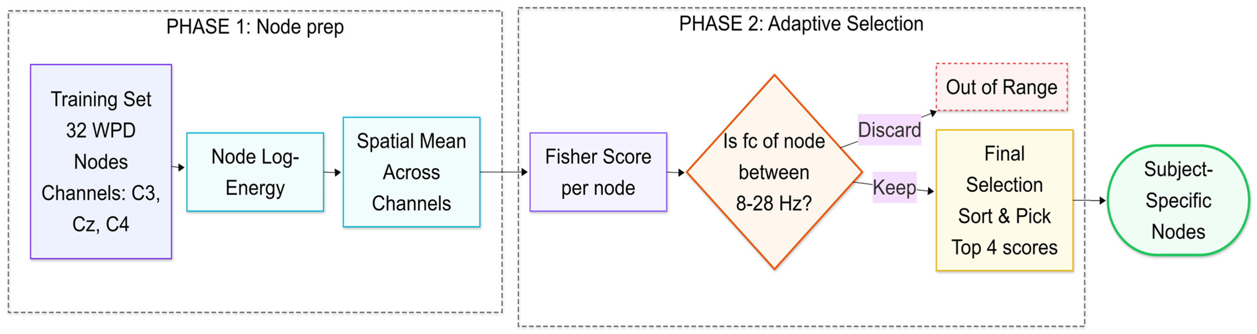
To ensure the system is robust against session-to-session variability and to prevent data leakage, a Fisher Firewall protocol is employed, where the data is split into training and testing sets prior to node selection. The selection process is governed by the following steps according to Figure 4:

The feature selection process is structured into two main phases to ensure the extracted features are both mathematically robust and physiologically relevant for motor imagery. In Phase 1, the Node Log-Energy is calculated for all 32 nodes to compress the signal’s dynamic range, followed by a spatial mean across channels (C3, Cz, and C4) to stabilize the features against single-channel noise. Phase 2 employs a Fisher Firewall protocol where the Fisher Score $\left(F{S}_n\right)$ for each node (n) is calculated using the training trials to measure the ratio of between-class variance to within-class variance as shown in Equation (11) [40]. This ensures the selection of nodes that are stable despite changes in subject mental state [24].

$$F{S}_n={\displaystyle \frac{{\displaystyle {\sum }_{k=1}^K}{n}_k({\mu }_{n,k}-{\mu }_{global}{)}^2}{{\displaystyle {\sum }_{k=1}^K}{n}_k({\sigma }_{n,k}^2+ϵ)}}$$

(11)

A spectral decision filters these results, discarding any nodes with a center frequency outside the 8–28 Hz range to eliminate non-physiological artifacts. The center frequency is constrained to 8–28 Hz to ensure the selected nodes are within the Mu and Beta rhythm. Equation (12) is used to determine the bandwidth of the node (bw) and to determine the center frequency ($f_{c,n})$ of the node with Equation (13).

$$bw={\displaystyle \frac{\frac{f_s}{2}}{2^l}}$$

(12)

where $f_s$ is the sampling rate and l is the decomposition level of 5.

$$f_{c,n}=\left(n+0.5\right)\times bw$$

(13)

This adaptive approach ensures that the feature set is precisely tuned to the individual’s unique spectral shifts, effectively mitigating the challenges of subject variability that often hinder BCI reliability. The extraction of multi-domain features comprising absolute power (Equation (14)), relative power (Equation (15)), and spatial variance ratios (Equation (16)) provides a comprehensive profile of the neural state [29]. While absolute power captures the intensity of frequency-specific oscillations, relative power normalizes these values against global brain noise to enhance the SNR. Furthermore, spatial variance ratios leverage the hemispheric lateralization inherent in motor imagery, ensuring the pipeline remains sensitive to the topographic shifts in Mu and Beta rhythms between the C3 and C4 cortical regions.

$$P_{abs}={log}_{10}(\sum w^2+ϵ)$$

(14)

$$P_{rel}={\displaystyle \frac{\sum w_{target}^2}{{\sum }_{n=1}^4\sum w_n^2+ϵ}}$$

(15)

$$\begin{gathered} R_{3,4}=\log \left(var\left(C_3\right)+ϵ\right)-\log \left(var\left(C_4\right)+ϵ\right) \\ {R}_{3,z}=\log \left(var\left(C_3\right)+ϵ\right)-\log \left(var\left(C_z\right)+ϵ\right) \\ {R}_{4,z}=\log \left(var\left(C_4\right)+ϵ\right)-\log \left(var\left(C_z\right)+ϵ\right) \end{gathered}$$

(16)

The features (3 features) are extracted from each node (4 nodes) from within C3, C4 and Cz (3 channels) for feature selection (36 features in total). To mitigate the impact of varying signal amplitudes between subjects, Z-score normalization is applied to the extracted features [41]. By calculating the mean and standard deviation from the training set and applying them to the test set, the pipeline ensures that the high-dimensional feature vector remains stable despite the fluctuations typically associated with long-term BCI use and participant fatigue.

3.6. Feature Selection

To optimize the high-dimensional feature vector extracted from the adaptive WPD, a GA was implemented to identify a subject-specific, optimal subset of features. This approach is designed to mitigate the complexity of MI signals while addressing session-to-session variability by selecting only the most stable and discriminative attributes [42,43].

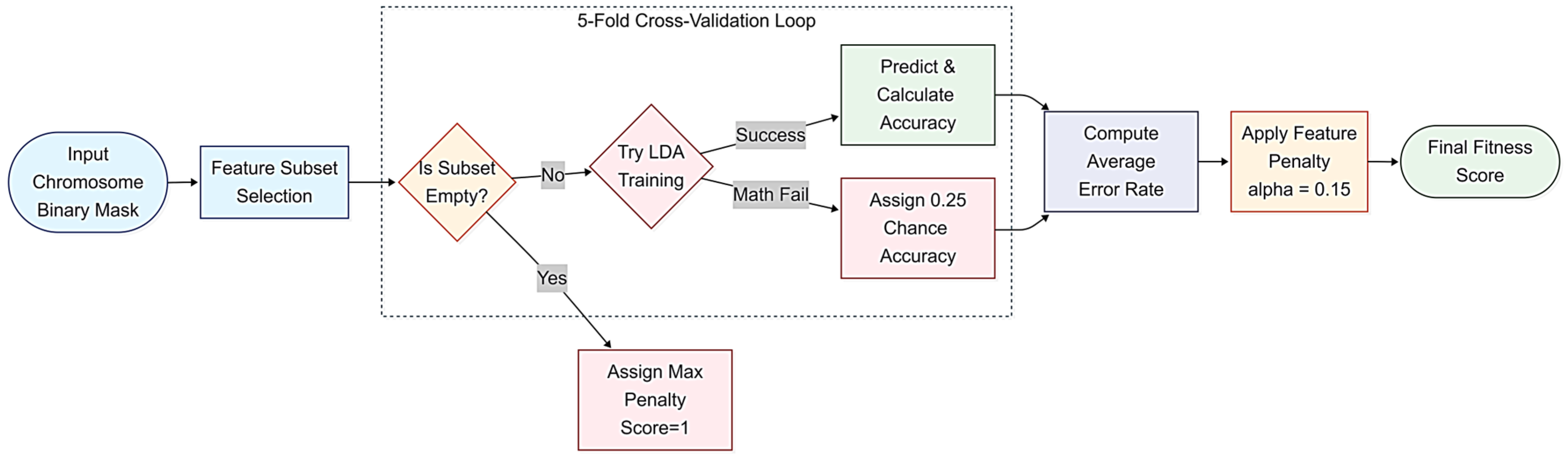
The GA was configured with a population size of 200 and evolved over 50 generations using scattered crossover and uniform mutation. A population size of 200 ensures sufficient genetic diversity to explore the high-dimensional feature space effectively. The number of generations was kept at 50 to ensure computational convergence within a small time limit, balancing optimization depth with the latency requirements of the real-time framework. To ensure the selection of an optimal feature set, a binary chromosome was constrained by lower (0) and upper (1) bounds. The fitness of each chromosome was evaluated using a composite fitness function shown in Figure 5, which minimized a combination of classification error and a feature count penalty:

• Accuracy: Determined via 5-fold cross-validation using an LDA classifier to avoid feature bias with the final classifiers. This internal cross-validation ensures that the feature selection process remains robust against overfitting and data leakage within the training set.
• (Penalty Factor): Set to 0.15 to penalize redundant features and favor low-dimensional subsets that reduce computational overhead for real-time BCI applications. This penalty factor serves as a dimensionality constraint, preventing the GA from chasing marginal gains in training accuracy that often result from overfitting. Instead, the algorithm is incentivized to prioritize the selection of robust, task-relevant feature subsets. By utilizing this subject-specific evolutionary search, the pipeline effectively isolates the synergistic interactions between the log-transformed power, relative power, and spatial ratios. This ensures that the final model is trained exclusively on features that exhibit the highest SNR for each participant, significantly improving the stability of the BCI MI predictions.

Figure 5. Flowchart of the Genetic Algorithm fitness function evaluation utilizing 5-fold cross-validation and LDA classification.

Figure 5. Flowchart of the Genetic Algorithm fitness function evaluation utilizing 5-fold cross-validation and LDA classification.

3.7. Classification

This study evaluates four distinct classification frameworks to establish a comprehensive performance baseline. K-Nearest Neighbors (KNN), Support Vector Machines (SVM), and Decision Trees serve as traditional, feature-based benchmarks that reflect established standards in MI classification. These models provide a rigorous comparison for a modified EEGNet, a deep learning architecture adapted to refine pre-selected MI features. EEGNet was selected over modern, high-capacity CNN architectures because its compact, task-specific design is optimized for the low-latency requirements of real-time BCI. Compared to deeper, more complex models that often introduce prohibitive computational overhead and black-box limitations, EEGNet provides the optimal balance of non-linear feature refinement and efficiency necessary for practical, clinical deployment. By evaluating both classical machine learning and a compact deep learning architecture, this analysis assesses the trade-offs between heuristic-driven feature engineering and automated non-linear refinement within the constraints of real-time, low-latency BCI applications.

3.7.1. KNN

The KNN algorithm is a non-parametric, instance-based learning method used for classifying complex biomedical signals. Compared to discriminative models that build a global mathematical formula, k-NN relies on local density estimation within a high-dimensional manifold [29,44,45]. In this study, the training phase establishes a reference using the features optimized by a GA. This process maps labeled MI trials into a multidimensional space to index the geometric boundaries between tasks.

Classification is performed by projecting the unseen test samples into the model and evaluating their proximity to the k most adjacent training instances using the Cityblock distance metric defined by Equation (17). With k = 3, the final class is assigned based on the majority vote among the 3 nearest neighbors. This hyperparameter choice serves as the primary mechanism for tuning sensitivity; using k = 3 allows the model to capture intricate local patterns, though it increases vulnerability to stochastic noise compared to a larger k, which improves generalization across the 30% test set by smoothing decision boundaries [46,47].

$$d\left(p, q\right)={\displaystyle {\sum }_{i=1}^n}\left|p_i-q_i\right|$$

(17)

3.7.2. SVM

SVM is a well-established machine learning algorithm used for both classification and regression. The method categorizes data points, referred to as support vectors, by designing a hyperplane that separates the data into distinct categories. This hyperplane is positioned to provide the correct separation class based on the geometric characteristics of the dataset, with the optimal hyperplane selected to maximize the margin between classes. Data are then assigned to a specific class depending on which side of the hyperplane it is located. Standard SVMs are inherently binary classifiers; an Error-Correcting Output Codes (ECOC) framework is used to scale the algorithm for multi-class MI classification. The ECOC model achieves this by training an ensemble of binary SVM classifiers using a coding design, such as one-versus-one, to accurately distinguish between multiple independent categories [29,44,45,48].

To design this hyperplane, the Radial Basis Function (RBF) kernel and C parameter of 2 were employed in this study. The region closest to the support vectors of groups +1 and −1 defines the slab’s edge, and the maximum margin is achieved within the area enclosed by the hyperplane. By applying appropriate techniques to recognize these support vectors, the margin can be increased to its fullest extent to enhance classification performance [49]. Under this configuration, the algorithm generates a model that finds decision boundaries to separate the motor imagery data into categories based on its spatial distribution.

3.7.3. Regression Tree

As a supervised learning framework, Decision Trees utilize a tree-like structure of nodes and branches to map input features to discrete class labels. Each internal node represents a specific feature test, while the branches represent the outcome of those tests, leading down to the final leaf nodes [50]. In BCI applications, these models are valued for their transparency but require careful management due to their greedy approach to data splitting. Post-pruning is utilized to enhance robustness by evaluating the tree against a validation set and trimming nodes that capture non-essential variance. To achieve this optimized stability, tailored structural parameters were explicitly defined instead of relying on standard default configurations. The parameters used are by setting the maximum number of branch splits to 15, requiring a minimum of 5 observations per leaf node, and employing the Gini Diversity Index (GDI) as the splitting criterion.

3.7.4. Modified EEGNet

EEGNet is a compact convolutional neural network architecture specifically designed to encapsulate the traditional feature engineering principles of the Filter Bank Common Spatial Pattern (FBCSP) framework within a deep learning structure. It typically utilizes 1-D temporal convolutions to act as a frequency filter bank, depth-wise convolutions to learn spatial filters across the scalp, and separable convolutions to weight and mix these characteristics for final classification [51,52]. In this study, the architecture is adapted into a Feature-Domain EEGNet (hybrid architecture) by replacing these raw-signal processing layers with compact, high-level kernels. While the original EEGNet is optimized for raw temporal signals, this adaptation was necessary to maintain input compatibility with our GA-optimized feature space. By utilizing the spatial and spectral refinement achieved through BSS and GA-optimized feature selection, the modified hybrid architecture eliminates the need for redundant filtering layers, thereby yielding a significant reduction in parameter count, as detailed in

Table 2. Layer properties and parameter configurations of the modified EEGNet hybrid architecture.

Layer Index	Name	Layer Type/Block	Filter/Kernel Size	Stride/Padding	Output Shape(H × W × C)	Operational Description and Purpose
1	‘Input’	Image Input Layer	-	-	1 × numF × 1	Receives the 4D reshaped vector of pre-selected GA features; applies zero-center normalization to stabilize early-stage gradients.
2	‘Conv_Features’	2D Convolution	1 × 3	Stride: 1 × 1 Padding: ‘same’	1 × numF × 32	Scans across adjacent pre-selected feature columns to extract local pattern correlations.
3	‘BN1’	Batch Normalization	-	-	1 × numF × 32	Normalizes intermediate activations; mitigates internal covariate shift across training mini-batches.
4	‘ReLU1’	Rectified Linear Unit	-	-	1 x numF x 32	Implements non-linear thresholding to preserve discriminative MI traits.
5	‘Conv_Global’	2D Convolution	1 × 5	Stride: 1 × 1 Padding: ‘same’	1 × numF × 64	Broadens the horizontal receptive field to detect global time-frequency combinations among the features.
6	‘BN2’	Batch Normalization	-	-	1 × numF × 64	Stabilizes downstream feature scaling prior to dimensional downsampling.
7	‘ReLU2’	Rectified Linear Unit	-	-	1 × numF × 64	Secondary activation mapping to enforce sparse, highly defined feature representation.
8	‘AvgPool’	Average Pooling	1 × 2	Stride: 1 × 2 Padding: 0	1 [numF/2] × 64	Downsamples the feature width via linear smoothing to suppress residual session-to-session and subject noise.
9	‘Dropout’	Dropout Regularization	-	-	1 × [numF/2] × 64	Randomly deactivates 40% (p = 0.4) of nodes per iteration to combat over-fitting across small sample sets.
10	‘FC_Output’	Fully Connected (Dense)	-	-	1 × 1 × numC	Maps the high-dimensional optimized feature map directly down to the targeted multi-class space.
11	‘Softmax’	Softmax Activation	-	-	1 × 1 × numC	Computes a normalized probability distribution across the independent motor imagery categories.
12	‘Output_Layer’	Cross-Entropy Loss	-	-	-	Computes categorical cross-entropy error metrics during model backpropagation.

, where numF represents the number of features and numC represents the number of classes. This results in a streamlined, low-latency model that focuses exclusively on the non-linear refinement of pre-selected MI features, making it ideal for stable, real-time BCI applications. Appendix A 

Table A3. Training options and optimization parameters for the modified EEGNet architecture.

Optimization Hyperparameter	Configuration Setting	Rationale
Solver Algorithm	Stochastic Gradient Descent with Momentum (‘sgdm’)	Provides smooth parameter trajectories to escape local minima in uncurated feature spaces.
Maximum Epoch Limit	100	Limits total execution length, terminating training before the network over-fits to non-neural residual components.
Mini-Batch Size	32	Optimized profile scaled to handle expanded data pools resulting from noise injection.
Initial Learning Rate	0.001	Conservative baseline parameter chosen to prevent catastrophic early gradient divergence.
Learning Rate Schedule	Piecewise decay (‘piecewise’)	Dynamically tightens solver stepping precision as network optimization nears a convergence plateau.
Drop Period and Drop Factor	Decreases by 0.5 every 30 epochs	Drops learning rate by half at structural milestones to safely resolve fine-grained hyperplane choices.
L2 Regularization (Weight Decay)	0.02	Balances weight penalty constraints to regularize loss boundaries against data scarcity.
Data Shuffling Paradigm	Shuffled every epoch (‘every-epoch’)	Breaks localized sequencing dependencies across trials to protect against cross-trial validation leakage.
Validation Frequency	Evaluated every 10 iterations	Provides granular, periodic diagnostic checks on training progress and generalization trends.
Validation Patience	Infinite patience (inf)	Forces full completion of the 100 epochs to establish a steady baseline for structural analysis without early-termination bias.

lists the training parameters and hyperparameters used to train the modified EEGNet model.

3.8. Performance Metrics

The diagnostic efficacy of the proposed BCI framework is evaluated using a suite of metrics derived from the confusion matrix. Given the four-class nature of the motor imagery task, all performance indicators are calculated using a macro-averaged, one-versus-rest (OvR) approach, ensuring that each class is weighted equally regardless of sample distribution [53]:

Accuracy: The proportion of total samples correctly classified across all four classes, represented by Equation (18):

$$Accuracy= {\displaystyle \frac{{\sum }_{i=1}^K{TP}_i}{Total Samples}}$$

(18)

where K = 4 represents the number of classes.

F1-Score: Harmonic mean of Precision and Recall, providing a balanced assessment of the model’s performance, represented by Equation (19):

$$F1\text{-}score= 2 · {\displaystyle \frac{Precision · Recall}{Precision+Recall}}$$

(19)

Precision: The macro-averaged accuracy of positive predictions, calculated as the mean of the class-specific precisions represented by Equation (20):

$$Precision= {\displaystyle \frac{1}{K}}{\displaystyle \sum _{i=1}^K}({\displaystyle \frac{{TP}_i}{{TP}_i+{FP}_i}})$$

(20)

Recall: The macro-averaged completeness of the model, measuring the ability to detect actual occurrences of each task represented by Equation (21):

$$Recall= {\displaystyle \frac{1}{K}}{\displaystyle \sum _{i=1}^K}({\displaystyle \frac{{TP}_i}{{TP}_i+{FN}_i}})$$

(21)

Cohens Kappa: Quantified by the percentage agreement between the actual experimental trials and the estimated labels produced by the classification output represented by Equation (22):

$$k= {\displaystyle \frac{P_o-P_c}{1-P_c}}$$

(22)

where $P_o$ is the relative observed agreement and $P_c=0.25$ is the hypothetical probability of chance agreement.

Area Under the Curve (AUC): A threshold-independent metric that quantifies the classifier’s discriminative capability. In the multiclass setting, the macro-averaged AUC is reported, calculated as the mean of the area under the ROC curve for each class versus all others. This provides a robust measure of performance that is less sensitive to class imbalance than point-based metrics.

3.9. Experimental Setup

The experimental pipelines were developed using MATLAB R2017b to maintain a consistent computational environment. To ensure a robust and leak-free evaluation, the pipeline was executed through a strictly sequenced workflow that separates global, unsupervised processing from supervised model development:

• Global Stochastic Augmentation: A global, label-preserving data augmentation stage was implemented. As detailed in Section 3.4.2, stochastic Gaussian noise injection was applied to the entire dataset to increase feature space density. This process is entirely unsupervised and label-blind, relying on signal-specific characteristics to generate synthetic variants without introducing label-dependent bias.
• Trial-Level Partitioning: The dataset was partitioned into a 70% training set and a 30% testing set at the trial level before feature extraction.
• Supervised Optimization (Training-Exclusive): This stage constitutes the supervised learning component of the pipeline. To isolate motor imagery (MI) activity, the analysis was restricted to the C3, C4, and Cz channels. Within this channel space, all operations sensitive to class discriminability, specifically the identification of optimal WPD nodes and the GA-optimized feature selection, were performed exclusively on the training partition.
• Fixed Transformation (Testing): The normalization parameters and optimized feature masks derived during the training phase were applied as fixed, independent transforms to the testing trials.

By restricting all supervised optimization and feature selection to the training data, the study ensures that the testing set remains a strictly independent hold-out.

4. Results

This section presents a systematic comparative evaluation of the three developed BCI pipelines: No-BSS pipeline, ICA pipeline, and EMD pipeline with a specific focus on their ability to mitigate low SNR and high session-to-session variability. By assessing performance across a diverse pool of nine subjects from the BCI Competition IV Dataset 2A described in Section 4.1 and the PhysioNet EEG MI dataset described in Section 4.2, these results demonstrate how different mathematical approaches handle the non-stationarity of MI signals. The analysis follows a triple-layer structure, examining dimensionality efficiency, multi-model classification accuracy, and computational efficiency to identify the most robust configuration and a comparative analysis with existing methodologies.

4.1. BCI Competition IV Dataset 2A Results

4.1.1. Dimensionality Efficiency

Feature space configurations were evaluated across the three pipelines: No-BSS Baseline (

Table 3. Spatio-spectral node selection and feature dimensionality per subject in No-BSS pipeline in BCI Competition IV Dataset 2A.

	A01	A02	A03	A04	A05	A06	A07	A08	A09
Optimal Nodes	2 3 5 6	6 4 5 3	2 3 6 4	5 6 3 2	3 6 5 4	2 6 3 5	5 6 3 4	3 2 6 4	3 2 5 6
Number of Features	12	10	12	18	12	7	14	11	15

), ICA (

Table 4. Spatio-spectral node selection and feature dimensionality per subject in ICA pipeline in BCI Competition IV Dataset 2A.

	A01	A02	A03	A04	A05	A06	A07	A08	A09
Optimal Nodes	2 3 5 6	6 4 5 3	2 3 6 5	5 6 4 3	2 5 3 6	6 2 5 4	6 5 4 2	3 5 2 4	3 2 5 6
Number of Features	10	16	12	12	11	6	11	12	9

), and EMD (

Table 5. Spatio-spectral node selection and feature dimensionality per subject in EMD pipeline in BCI Competition IV Dataset 2A.

	A01	A02	A03	A04	A05	A06	A07	A08	A09
Optimal Nodes	2 3 5 6	4 6 3 2	2 3 6 4	5 6 3 2	3 6 4 2	2 6 3 5	5 6 3 2	3 2 6 4	3 2 5 6
Number of Features	12	4	10	9	13	14	12	12	10

) for a nine-subject cohort. By utilizing WPD sub-band node selection with the Fisher Score restricted to the 8–28 Hz range, the architecture maximized the ratio of between-class to within-class variance, potentially accommodating subject-specific spectral shifts that may arise from individual anatomical variations, such as skull thickness or cortical geometry. The architecture simultaneously preserved stable sub-band locking across all pipelines, including the baseline, in specific subjects like A01 and A09. The GA operated as a spatial optimizer, evaluating a total pool of 36 features for each subject to isolate the most discriminative subset. Final feature counts exposed pipeline-dependent spatial complexity trends compared directly against the No-BSS baseline. EMD pipeline either allowed dimensional compression by concentrating signal energy or necessitated feature inflation to mitigate mode-mixing artifacts. In contrast, ICA consistently increased spatial complexity due to the spatial dispersion of task-relevant signatures following artifact back-projection. Appendix A (

Table A1. Frequency partition of WPD nodes at level 5 for Alpha and Beta bands (fs = 250 Hz).

Node (l = 5)	Centre Frequency of Node	Frequency Range	Physiological Band
0	1.95 Hz	0–3.91 Hz	Delta
1	5.86 Hz	3.91–7.82 Hz	Theta
2	9.77 Hz	7.82–11.73 Hz	Alpha
3	13.68 Hz	11.71–15.64 Hz	Low Beta
4	17.59 Hz	15.64–19.55 Hz	Beta
5	21.50 Hz	19.55–23.46 Hz	Beta
6	25.41 Hz	23.46–27.37 Hz	Beta
7	29.32 Hz	27.37–31.28 Hz	High Beta/Gamma

) provides the complete mapping of calculated time-frequency nodes, bandwidths, and frequency ranges across all subjects and pipelines. The table columns detail the decomposition level, specific node index, corresponding center frequency (Hz), and the resulting bandwidth, providing a comprehensive reference for interpreting the performance metrics reported in Table 3, Table 4 and Table 5.

4.1.2. Within-Subject Multi-Model Analysis

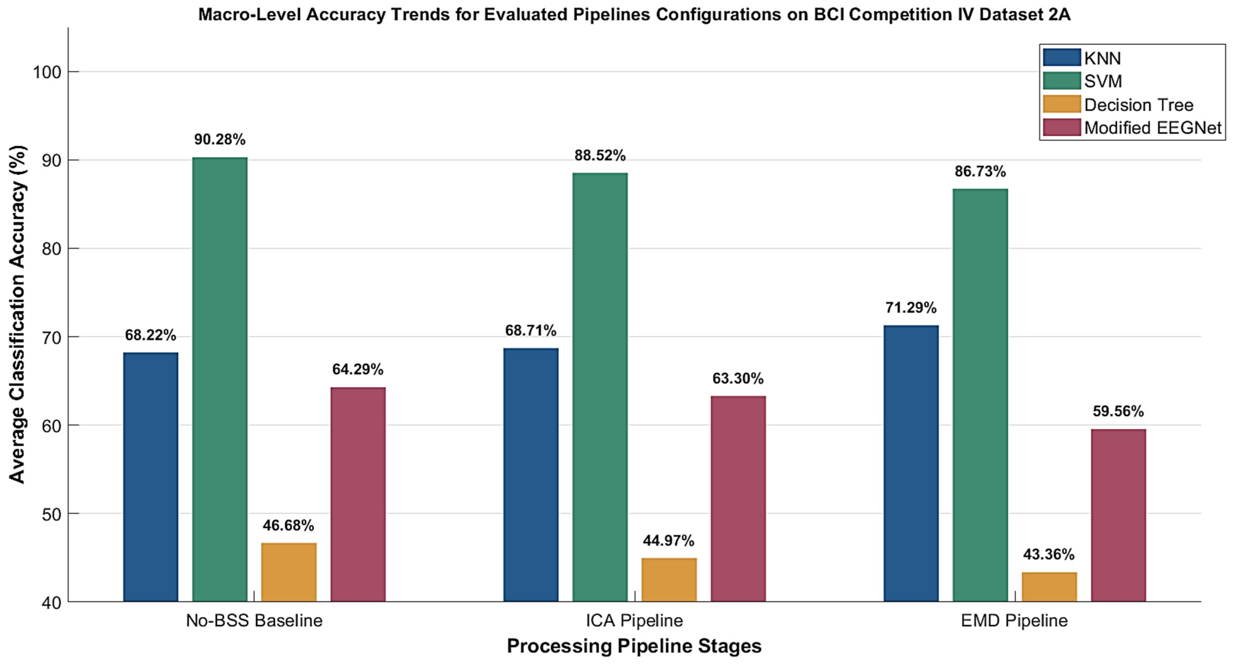
Classification performance was evaluated using a within-subject strategy across the 9-subject cohort, comparing KNN, SVM, Decision Tree, and a modified EEGNet model. As shown in Figure 6, the SVM consistently outperformed other classifiers, delivering the highest individual decoding accuracies with the lowest intra-subject variance. Within the No-BSS baseline pipeline, the SVM reached 90.28% accuracy, outperforming KNN, modified EEGNet, and Decision Trees. This robust baseline performance highlights the utility of the SVM’s maximum-margin hyperplane in mapping distinct MI class boundaries from localized, subject-specific channel covariance matrices. These findings demonstrate the pipeline’s efficacy when optimized for individual participants, rather than in cross-subject scenarios.

Observing the cross-pipeline macro-trends in Figure 6 reveals a divergence in how these frameworks respond to preprocessing. While advanced preprocessing caused a slight decline in SVM performance, the KNN model experienced progressive improvements, increasing by ~0.5% with ICA and peaking with a ~3% improvement over baseline when using EMD. In contrast, the Decision Tree and modified EEGNet models showed minimal sensitivity to these preprocessing changes, maintaining relatively static performance tiers. This suggests that the spatial unmixing and sifting processes primarily benefit distance-based decision boundaries by removing non-stationary artifact noise and tightening geometric feature clusters.

To evaluate the statistical significance of performance differences between the No-BSS baseline and conventional ICA and EMD pipelines, a two-tailed paired $t$-test was utilized. This allowed for direct, within-subject comparisons, controlling for inter-subject variability by evaluating each pipeline on identical data splits. Differences were considered statistically significant at 0.05. As shown in

Table 6. Pairwise p-values comparing the No-BSS baseline against BSS-based pipelines in BCI Competition IV Dataset 2A.

	KNN	SVM	Decision Tree	Modified EEGNet
No-BSS vs. EMD	0.054	0.088	0.409	0.033
No-BSS vs. ICA	0.811	0.082	0.637	0.643

, the majority of the pairwise comparisons yielded $p$-values > 0.05, indicating that the performance differences between the No-BSS pipeline and traditional BSS-based pipelines are not statistically significant. These results demonstrate that the No-BSS baseline achieves classification accuracy comparable to traditional ICA or EMD pipelines. This indicates that adaptive spatial filtering and GA-optimized feature selection are sufficient to capture discriminative neural markers, effectively rendering the computational burden of BSS-based preprocessing redundant.

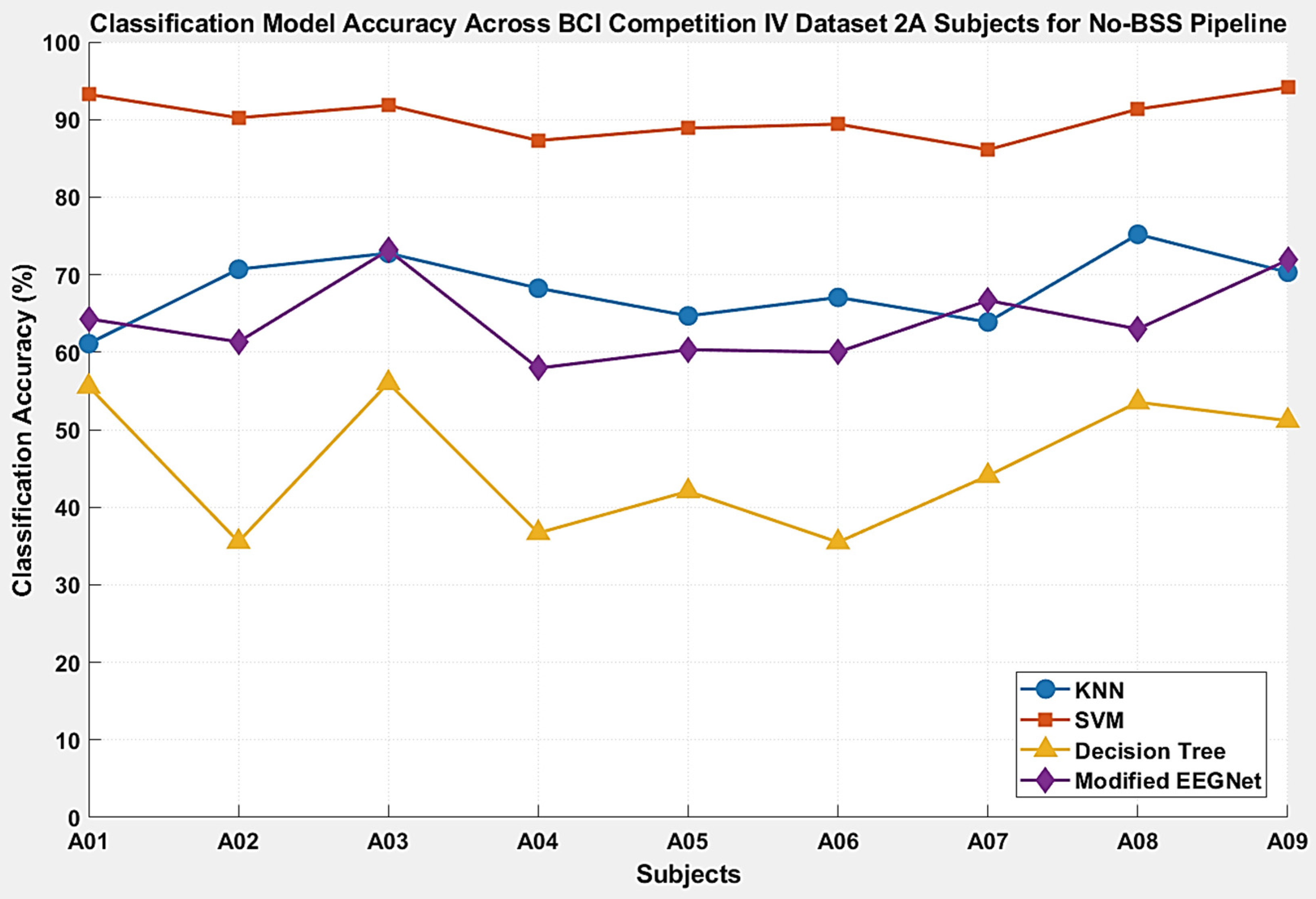
Analyzing subject-level trends reveals how pipelines dynamically adapt to individual profiles. No-BSS baseline establishes performance benchmarks (Figure 7 and

Table 7. Comparative classification accuracy across multiple architectures for No-BSS pipeline in BCI Competition IV Dataset 2A.

	A01	A02	A03	A04	A05	A06	A07	A08	A09	Average
KNN	61.11%	70.70%	72.76%	68.25%	64.68%	67.06%	63.89%	75.20%	70.31%	68.22% ± 4.26%
SVM	93.25%	90.23%	91.83%	87.30%	88.89%	89.41%	86.11%	91.34%	94.14%	90.28% ± 2.50%
Decision Tree	55.56%	35.55%	56.03%	36.68%	42.06%	35.49%	44.05%	53.54%	51.17%	46.68% ± 7.36%
Modified EEGNet	64.29%	61.33%	73.15%	57.94%	60.32%	60.00%	66.67%	62.99%	71.88%	64.29% ± 5.02%

), where high-proficiency users (A01, A03, A08, A09) serve as anchors. Their robust ERD modulations and potential cranial geometries minimize volume conduction, enabling simpler models like KNN to maintain elevated results. In contrast, A02 and A06 present complex challenges: A06 exhibits severe signal attenuation, while A02 demonstrates high sensitivity to signal non-stationarity.

The Adaptive Laplacian spatial filter is important here, dynamically adjusting weights to match individual neural patterns, eliminating background noise while preserving core MI rhythms. This balance is essential, as an overly aggressive filter would attenuate the faint neural signatures of subjects like A06, degrading accuracy. Instead, the filter’s adaptive nature regularizes the feature space for the classifier. The design’s efficacy is confirmed by the SVM’s maximum-margin hyperplane, which normalizes these difficult profiles, elevating A02 and A06 by over 50% from baseline to join the high-performance bracket shared by the rest of the cohort. This convergence validates the pipeline as a universal physiological equalizer, removing interference without compromising the critical trial-level details required for stable, cohort-wide decoding (~90% average).

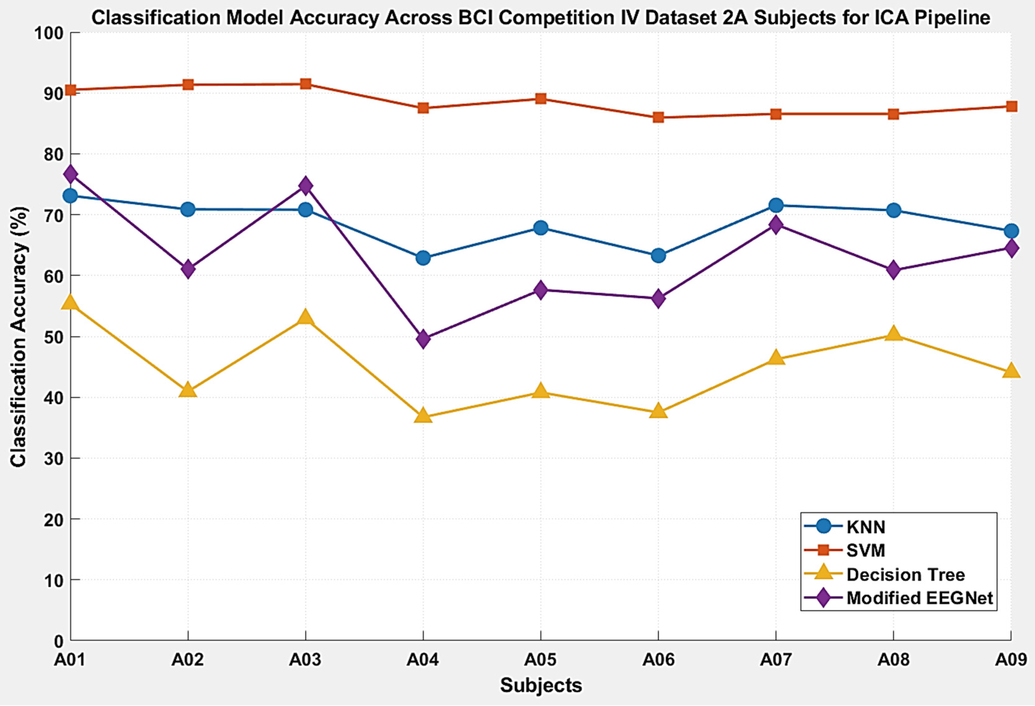
In the ICA configuration, the algorithm functions as a global spatial preprocessing stage to isolate artifact sources before feature extraction. Figure 8 and

Table 8. Comparative classification accuracy across multiple architectures for ICA pipeline in BCI Competition IV Dataset 2A.

	A01	A02	A03	A04	A05	A06	A07	A08	A09	Average
KNN	73.12%	70.87%	70.82%	62.89%	67.84%	63.28%	71.54%	70.71%	67.32%	68.71% ± 3.45%
SVM	90.51%	91.34%	91.44%	87.50%	89.02%	85.94%	86.56%	86.56%	87.80%	88.52% ± 2.02%
Decision Tree	55.34%	40.94%	52.92%	36.72%	40.78%	37.50%	46.25%	50.20%	44.09%	44.97% ± 6.31%
Modified EEGNet	76.68%	61.02%	74.71%	49.61%	57.65%	56.25%	68.38%	60.87%	64.57%	63.30% ± 8.28%

illustrate the pipeline’s capacity to stabilize performance across diverse neurophysiological profiles. High-proficiency users (A01, A03, A08) remain performance anchors, allowing simpler models like KNN to maintain consistent classification results. In contrast, A02 and A06 highlight the boundaries of this global spatial filter. Subject A06 exhibits limited classification performance, suggesting that MI rhythms may be attenuated potentially by factors like localized skull impedance. In contrast, A02 reacts dynamically; while this subject shows high sensitivity to signal non-stationarity, the clean extraction of true neural components enables the system to isolate core MI patterns. The performance gap between the baseline Decision Tree and the optimized SVM highlights that, even with ICA, signal complexity necessitates a maximum-margin hyperplane for effective mapping. Integrating the Adaptive Laplacian filter as a secondary refinement layer further enhances the MI signal. This approach avoids the risk of over-filtering, which would otherwise discard important neural rhythms. This processing allows the SVM to normalize difficult profiles like A02 and A06 into the high-performance bracket, validating the pipeline’s ability to resolve biological non-stationarity while preserving trial-level features cohort-wide.

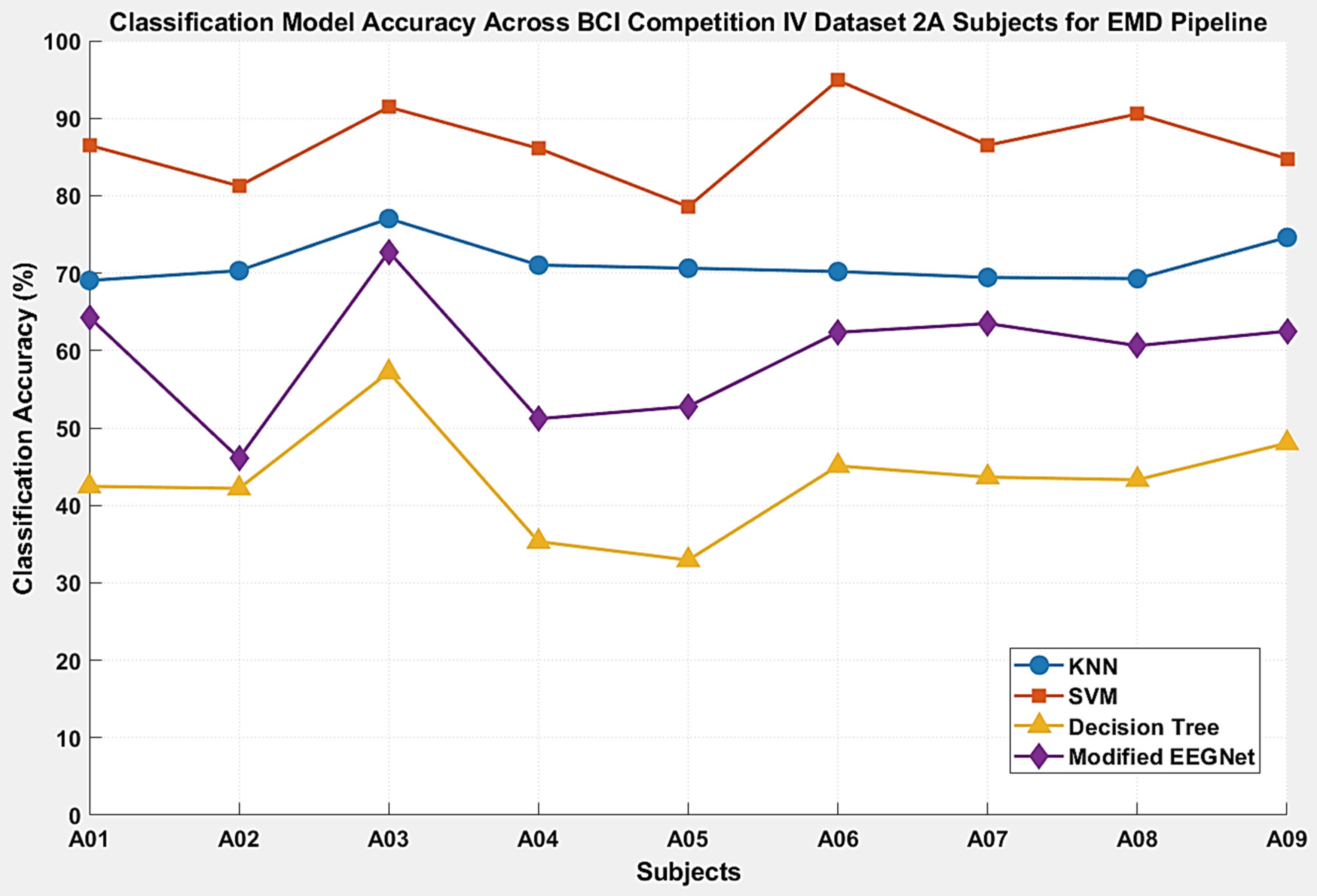
In the EMD configuration, the algorithm acts as a data-driven, non-linear temporal filter, decomposing EEG data into IMFs before feature extraction, as shown in Figure 9 and

Table 9. Comparative classification accuracy across multiple architectures for EMD pipeline in BCI Competition IV Dataset 2A.

	A01	A02	A03	A04	A05	A06	A07	A08	A09	Average
KNN	69.05%	70.31%	77.04%	71.03%	70.63%	70.20%	69.44%	69.29%	74.61%	71.29% ± 3.42%
SVM	86.51%	81.25%	91.44%	86.11%	78.57%	94.90%	86.51%	90.55%	84.77%	86.73% ± 3.42%
Decision Tree	42.46%	42.19%	57.20%	35.32%	32.94%	45.10%	43.65%	43.31%	48.05%	43.36% ± 6.60%
Modified EEGNet	64.29%	46.09%	72.76%	51.19%	52.78%	62.35%	63.49%	60.63%	62.50%	59.56% ± 7.65%

. Compared to global spatial filters, EMD isolates oscillatory components directly in the time domain. For the high-proficiency user (A03), this effectively isolates MI rhythms, enabling the KNN and SVM to reach their highest accuracy tiers. However, EMD’s time-frequency fragmentation reveals distinct trade-offs. While the pipeline yields peak performance for subjects like A06, it degrades accuracy for A02, whose non-stationary signal distribution interacts poorly with rigid feature mapping. This structural mismatch is most evident in the modified EEGNet, where unconstrained temporal decomposition destabilizes network optimization in volatile subjects.

To mitigate over-aggressive decomposition, signal fragmentation, and mode mixing, the EMD sifting process was constrained to two iterations. This is important, as EMD alters temporal characteristics and shifts the spectral landscape that the WPD must navigate. By limiting sifting, the pipeline preserves structural integrity, ensuring the WPD selects nodes representing true neural rhythms rather than artifacts. This synchronization allows the SVM to bypass baseline failures, yielding substantial accuracy gains exceeding 50% for difficult subjects and stabilizing overall cohort performance.

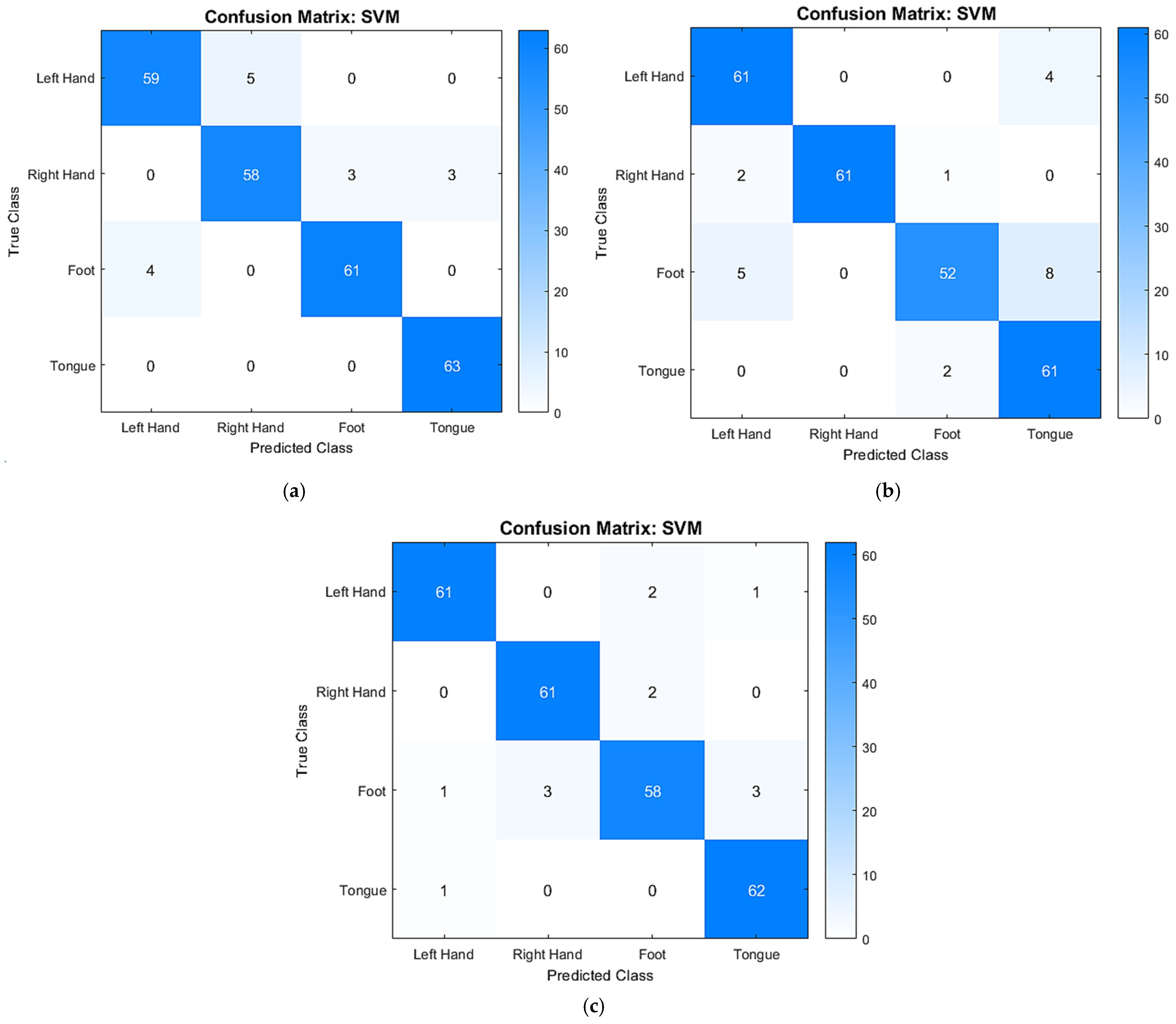
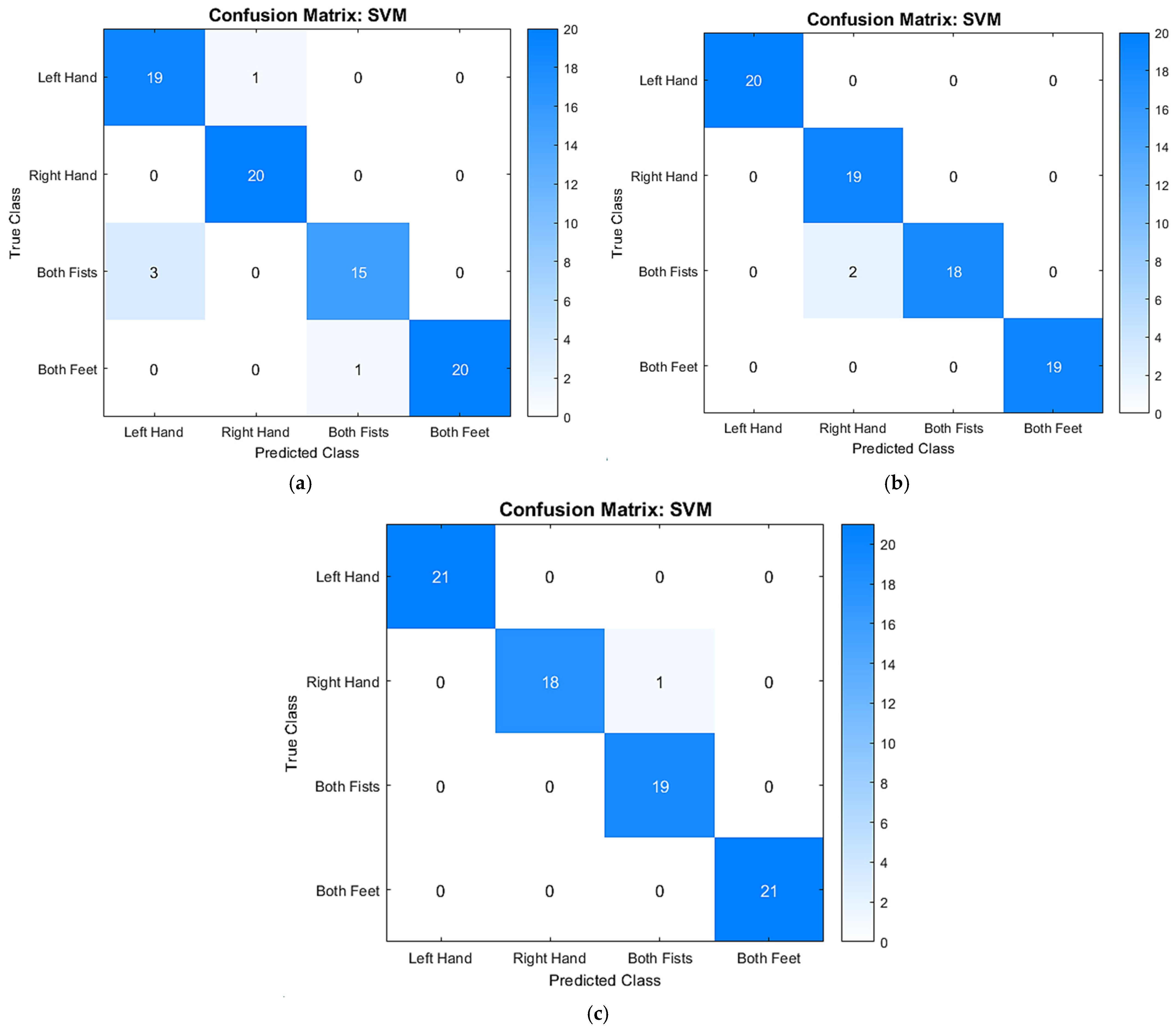
The diagonal alignment of hit-rates across the target classes confirms that the adaptive WPD successfully isolates authentic MI intent across different subjects, rather than relying on class-bias artifacts. Average accuracy metrics often mask the underlying causes of classification errors, as a high score does not clarify whether a model is effectively distinguishing between classes or merely favoring dominant patterns. To provide a more granular diagnostic assessment, confusion matrices were employed to visualize the distribution of true and false predictions across all four MI tasks. Furthermore, the top-performing subject profile from each pipeline is highlighted to establish the framework’s potential performance ceiling and to demonstrate its capacity to resolve complex class boundaries under optimal conditions, as shown in Figure 10. Within the No-BSS baseline pipeline in Figure 10a, Subject A09 establishes a robust foundation, demonstrating highly symmetric true-positive and true-negative distributions despite operating with no BSS. For a separate subject within the ICA pipeline in Figure 10b, Subject A03 achieves a near-flawless class separation of 91.44%, proving that independent source unmixing effectively eliminates transient ocular and muscle artifacts to uncover clean MI patterns. The absolute ceiling of the study is reached under the EMD pipeline in Figure 10c by Subject A06, securing a peak cohort accuracy of 94.90%. This outcome provides verification that decomposing non-stationary EEG into localized intrinsic modes successfully concentrates the targeted sensorimotor rhythm power. This allows the GA to compress the data down to a compact 11-feature topography where the SVM hyperplane maps entirely unambiguous class boundaries.

To assess the macro-level stability of the multi-model architectures, the study systematically analyzed cohort-wide metrics including Cohen’s Kappa, F1-Score, Recall, Precision, and AUC (

Table 10. Average performance metrics for KNN in BCI Competition IV Dataset 2A.

Performance Metrics	No BSS	ICA	EMD
Kappa	0.5761 ± 0.0569	0.5823 ± 0.0459	0.6171 ± 0.0342
F1-Score	0.6819 ± 0.0435	0.6868 ± 0.0345	0.7110 ± 0.0262
Recall	0.6820 ± 0.0423	0.6870 ± 0.0344	0.7128 ± 0.0259
Precision	0.6885 ± 0.0430	0.6870 ± 0.0357	0.7174 ± 0.0267
AUC	0.8989 ± 0.0201	0.8997 ± 0.0158	0.9052 ± 0.138

,

Table 11. Average performance metrics for SVM in BCI Competition IV Dataset 2A.

Performance Metrics	No BSS	ICA	EMD
Kappa	0.8704 ± 0.0333	0.8469 ± 0.0269	0.8231 ± 0.0636
F1-Score	0.9023 ± 0.0251	0.8849 ± 0.0202	0.8672 ± 0.0474
Recall	0.9028 ± 0.0250	0.8852 ± 0.0203	0.8673 ± 0.0477
Precision	0.9059 ± 0.0242	0.8885 ± 0.0197	0.8712 ± 0.0465
AUC	0.9733 ± 0.0086	0.9712 ± 0.0075	0.9596 ± 0.0230

,

Table 12. Average performance metrics for Decision Tree in BCI Competition IV Dataset 2A.

Performance Metrics	No BSS	ICA	EMD
Kappa	0.2935 ± 0.0929	0.2665 ± 0.0842	0.2443 ± 0.0886
F1-Score	0.4515 ± 0.0794	0.4365 ± 0.0699	0.4195 ± 0.0753
Recall	0.4697 ± 0.0696	0.4502 ± 0.0635	0.4331 ± 0.0666
Precision	0.5312 ± 0.0696	0.4803 ± 0.0695	0.4744 ± 0.0602
AUC	0.7140 ± 0.0576	0.7232 ± 0.0561	0.6837 ± 0.0606

and

Table 13. Average performance metrics for modified EEGNet in BCI Competition IV Dataset 2A.

Performance Metrics	No BSS	ICA	EMD
Kappa	0.5177 ± 0.0735	0.5107 ± 0.1103	0.4608 ± 0.0765
F1-Score	0.6418 ± 0.0515	0.6307 ± 0.0836	0.5946 ± 0.0761
Recall	0.6416 ± 0.0483	0.6334 ± 0.0827	0.5954 ± 0.0767
Precision	0.6457 ± 0.0505	0.6355 ± 0.0840	0.5969 ± 0.0763
AUC	0.8532 ± 0.0366	0.8533 ± 0.0496	0.8279 ± 0.0526

). Across all pipelines, uniform convergence was observed among F1-Score, Recall, and Precision. This alignment confirms that, despite minor class imbalances introduced during trial pruning, the optimized feature space remains robust and unbiased, yielding symmetric predictive sensitivity and specificity.

The within-subject SVM configuration consistently established the statistical ceiling across every evaluated metric. It maintained a high probabilistic capacity to isolate sensorimotor rhythms, evidenced by minimal standard deviations across all metrics, often below 0.05. While the SVM, Decision Tree, and modified EEGNet frameworks experienced sequential performance decreases when transitioning through the ICA and EMD pipelines, the SVM remained highly resilient, sustaining a high-performance bracket even after EMD sifting.

A distinct architectural variance emerged within the KNN model, which demonstrated a performance inversion compared to the other classifiers. Rather than degrading, the KNN model exhibited systematic improvements across all metrics under the EMD pipeline, with performance gains of approximately 7% to 10% above baseline and a marked tightening of standard deviations. This implies that the EMD sifting mechanism successfully isolates clean, spatio-spectral pockets from non-stationary EEG data. By organizing intrinsic mode components into distinct spatial neighborhoods, the EMD pipeline creates a compact distance-based topography that optimizes the instance-based mechanics of the KNN feature space, ensuring both higher accuracy and increased consistency.

4.2. PhysioNet EEG MI Dataset Results

4.2.1. Dimensionality Efficiency

The efficiency of the GA feature selection method was analyzed across three pipelines using nine subjects from the PhysioNet dataset. PhysioNet provides a demanding test environment as the signals were recorded raw, retaining original background noise like powerline interference, ocular artifacts, and muscle activity. To manage this, the WPD process was restricted to the 8–28 Hz alpha-beta band, acting as a targeted filter to isolate relevant MI characteristics. This approach identified stable, subject-specific signal patterns robust to inter-subject variability, evidenced by locked node patterns across individuals, such as subjects S001 and S002.

The GA scanned 36 feature combinations, revealing structural trends dependent on the preprocessing choice. Within the No-BSS baseline in

Table 14. Spatio-spectral node selection and feature dimensionality per subject in No-BSS pipeline in PhysioNet subset.

	S001	S002	S003	S004	S005	S006	S007	S008	S009
Optimal Nodes	6 8 7 5	5 6 8 7	9 8 10 5	4 5 10 7	4 7 3 5	4 6 5 3	3 6 9 8	6 5 8 7	9 5 3 10
Number of Features	14	13	10	21	22	15	17	19	15

, the system established initial feature counts. In contrast, the ICA pipeline in

Table 15. Spatio-spectral node selection and feature dimensionality per subject in ICA pipeline in PhysioNet subset.

	S001	S002	S003	S004	S005	S006	S007	S008	S009
Optimal Nodes	7 5 4 10	5 6 8 7	9 8 10 3	6 4 10 7	4 5 8 7	7 5 6 8	3 7 10 6	6 4 10 7	3 7 6 5
Number of Features	15	18	16	12	12	24	17	13	14

generally increased the required features across the cohort because signal reconstruction tends to spread relevant MI patterns across a wider network of channels. Under the EMD pipeline in

Table 16. Spatio-spectral node selection and feature dimensionality per subject in EMD pipelin in PhysioNet subset.

	S001	S002	S003	S004	S005	S006	S007	S008	S009
Optimal Nodes	6 8 9 7	8 5 10 9	9 8 10 3	5 4 10 6	4 7 3 8	6 4 5 3	3 7 6 8	6 5 4 10	5 7 3 10
Number of Features	10	15	12	19	18	21	11	15	19

, the cleaning process successfully concentrated signal information, allowing the GA to simplify the feature count for some subjects (S001 and S007). However, for others, localized noise variations forced the algorithm to select extra features to maintain performance, such as in S006. Appendix A 

Table A2. Frequency partition of WPD nodes at level 5 for Alpha and Beta bands (fs = 160 Hz).

Node (l = 5)	Centre Frequency of Node	Frequency Range	Physiological Band
0	1.25 Hz	0–2.5 Hz	Delta
1	3.75 Hz	2.5–5 Hz	Theta
2	6.25 Hz	5–7.5 Hz	Alpha
3	8.75 Hz	7.5–10 Hz	Low Beta
4	11.25 Hz	10–12.5 Hz	Beta
5	13.75 Hz	12.5–15 Hz	Beta
6	16.25 Hz	15–17.5 Hz	Beta
7	18.75 Hz	17.5–20 Hz	Beta
8	21.25 Hz	20–22.5 Hz	Beta
9	23.75 Hz	22.5–25 Hz	Beta
10	26.25 Hz	25–27.5 Hz	High Beta

serves as the reference for these results, demonstrating the inter-subject variability in MI signatures. The table columns detail the decomposition level, specific node index, corresponding center frequency (Hz), and the resulting bandwidth, providing a comprehensive reference for interpreting the performance metrics reported in Table 3, Table 4 and Table 5.

4.2.2. Within-Subject Multi-Model Analysis

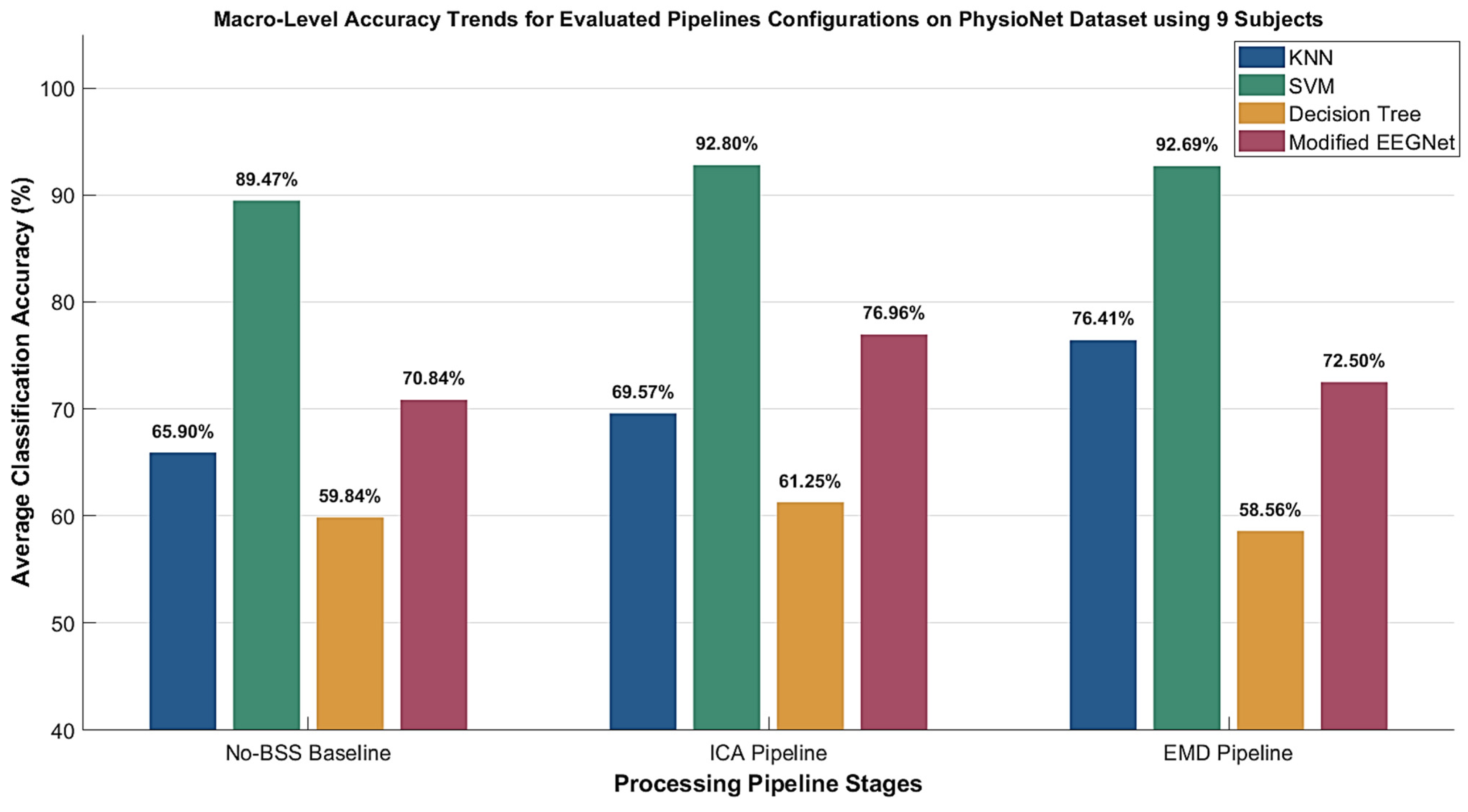
To evaluate the overall impact of the processing pipelines, the average classification accuracies for the four machine learning models across the nine-subject PhysioNet cohort are compared in Figure 11. A within-subject analysis reveals a clear performance hierarchy, influenced by how effectively each classifier navigates raw versus BSS-processed data. In the No-BSS baseline, the SVM establishes the statistical ceiling, demonstrating a superior capacity to ignore background noise compared to the modified EEGNet, KNN, and Decision Tree configurations.

Analyzing performance across the three pipelines reveals distinct behavioral contrasts. The SVM shows direct improvement when BSS techniques are introduced, reaching its peak accuracy with the ICA pipeline and maintaining that performance tier with EMD. This indicates that unmixing independent source artifacts and filtering non-stationary noise establishes sharper classification boundaries than standard filtering alone. Concurrently, the KNN model captures the most significant benefit from these advanced stages; its accuracy shows a substantial, step-by-step climb of over 10.5% from baseline to the EMD pipeline. This improvement highlights that extracting true independent components or intrinsic modes effectively clears the distortion that typically hinders local distance metrics in raw datasets. Meanwhile, the modified EEGNet maintains a steady, mid-range profile, peaking under ICA, while the Decision Tree remains bottlenecked by its architecture, exhibiting only minor performance fluctuations across all pipelines.

While the majority of comparisons showed no statistically significant differences, select exceptions were noted. Specifically, in the PhysioNet subset shown in

Table 17. Pairwise p-values comparing the No-BSS baseline against BSS-based pipelines in PhysioNet subset.

	KNN	SVM	Decision Tree	Modified EEGNet
No-BSS vs. EMD	<0.001	0.017	0.580	0.657
No-BSS vs. ICA	0.288	0.084	0.653	0.061

, the No-BSS pipelines differed from the EMD pipeline when using KNN and SVM classifiers. However, the broader trend, particularly the consistent performance difference with the ICA-based pipeline, demonstrates that the No-BSS pipeline is not statistically significant compared to traditional methods in most models. These isolated variations provide a subtle perspective without challenging the primary conclusion: that adaptive spatial filtering and GA-optimized feature selection are sufficient to achieve robust classification, effectively rendering intensive BSS preprocessing redundant.

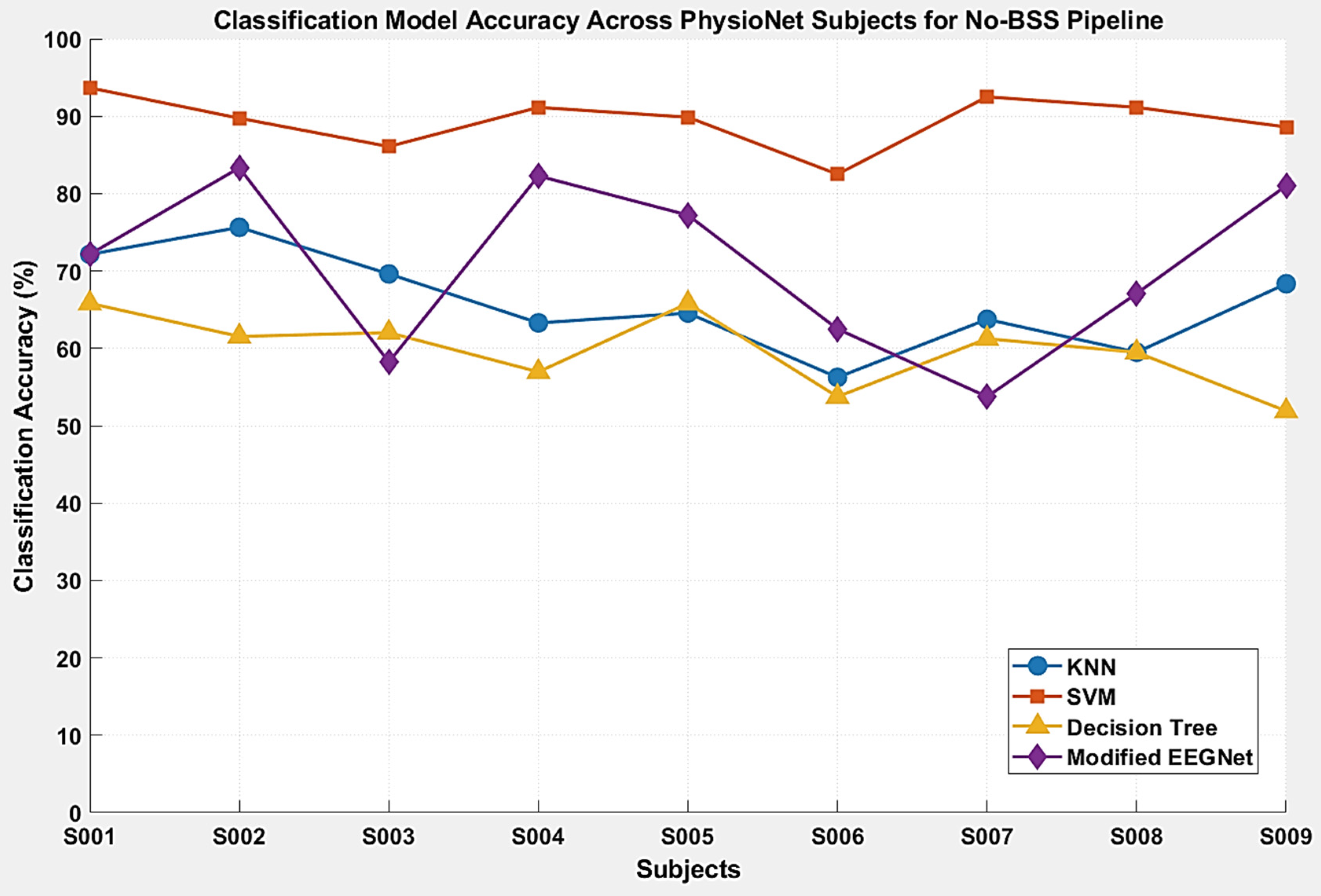
Examining subject-level results demonstrates how pipeline configurations adapt to subject-specific data to optimize classification. The No-BSS pipeline (Figure 12,

Table 18. Comparative classification accuracy across multiple architectures for No-BSS pipeline in Physionet subset.

	S001	S002	S003	S004	S005	S006	S007	S008	S009	Average
KNN	72.15%	75.64%	69.62%	63.29%	64.56%	56.25%	63.75%	59.49%	68.35%	65.90% ± 5.79%
SVM	93.67%	89.74%	86.08%	91.14%	89.87%	82.50%	92.50%	91.14%	88.61%	89.47% ± 3.22%
Decision Tree	65.82%	61.54%	62.03%	56.96%	65.82%	53.75%	61.25%	59.49%	51.90%	59.84% ± 4.59%
Modified EEGNet	72.15%	83.33%	58.23%	82.28%	77.22%	62.50%	53.75%	67.09%	81.01%	70.84% ± 10.34%

) establishes baseline performance, revealing trial-to-trial dynamics within the PhysioNet cohort High-proficiency users (S001, S004, and S007) serve as performance anchors, achieving high classification rates even in the absence of BSS. In contrast, S006 presents an attenuated signal profile, representing a physiological noise barrier. While simpler models like KNN and Decision Tree struggle with this signal, the SVM’s margin-maximizing properties, achieving over 80% accuracy confirm that essential MI rhythms remain preserved despite the lack of global spatial filtering.

Biological non-stationarity is most evident in the deep learning baseline. Subjects S003 and S007 demonstrate conflicting vulnerabilities. While S003’s performance degrades in the modified EEGNet, their KNN accuracy remains stable; in contrast, S007 shows a sharp collapse in EEGNet performance despite maintaining high separability for the SVM. These contrasting collapses highlight the sensitivity of deep learning architectures to subject-level volatility, further reflected by the cohort-wide standard deviation of 10.34%.

To mitigate these instabilities, the pipeline routes raw signals through the Adaptive Laplacian filter. By dynamically enhancing MI rhythms based on electrode-neighbor correlations, this spatial targeting regularizes the feature space. This ensures that even when uncleaned temporal features confuse convolutional or tree-based networks, the SVM can resolve a stable maximum-margin hyperplane. This approach effectively normalizes difficult profiles, such as S003 and S006, into an elevated performance bracket, demonstrating the pipeline’s resilience to intra-subject variability.

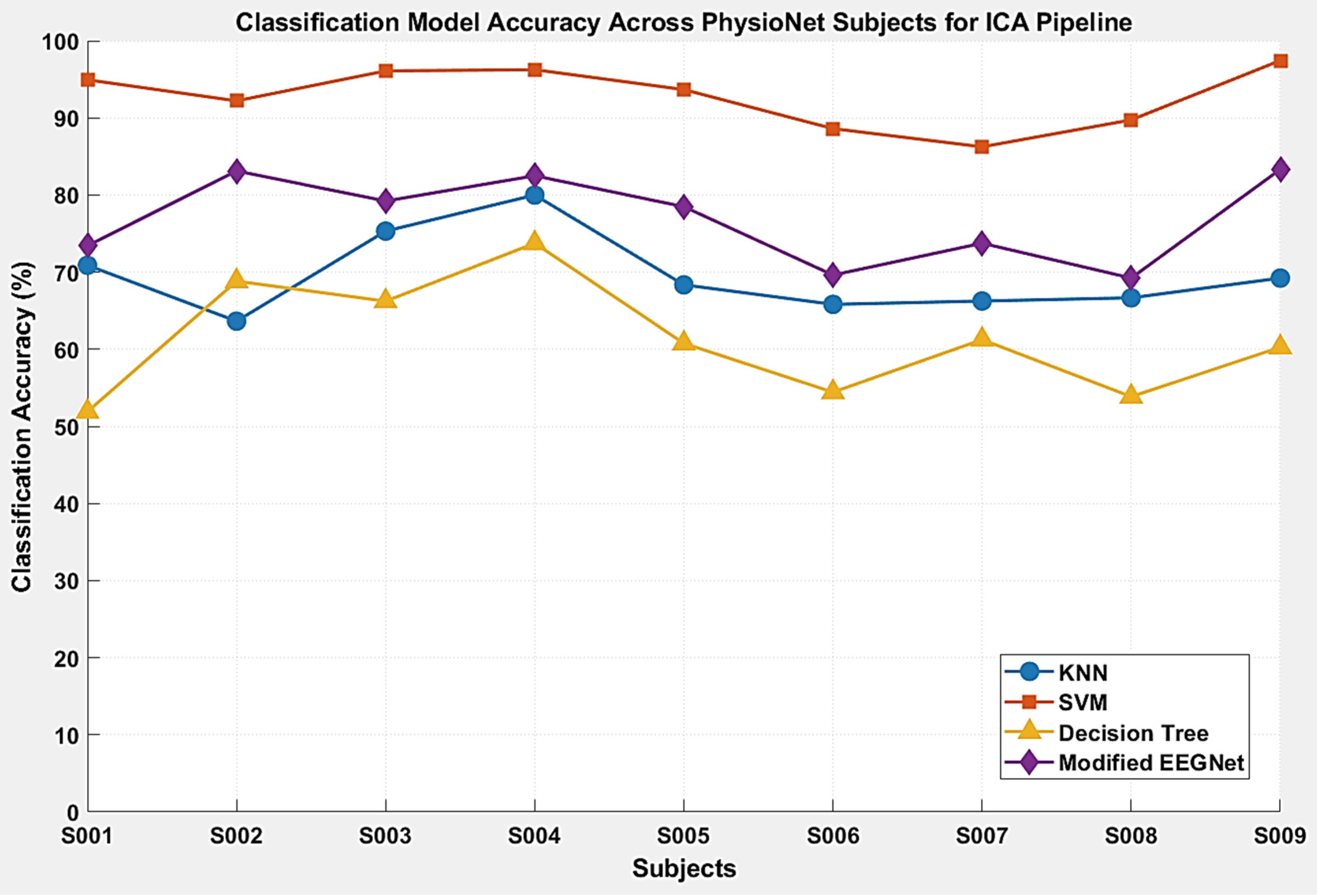
Under the ICA configuration (Figure 13,

Table 19. Comparative classification accuracy across multiple architectures for ICA pipeline in PhysioNet subset.

	S001	S002	S003	S004	S005	S006	S007	S008	S009	Average
KNN	70.89%	63.64%	75.32%	80.00%	68.35%	65.82%	66.25%	66.67%	69.23%	69.57% ± 4.88%
SVM	94.94%	92.21%	96.10%	96.25%	93.67%	88.61%	86.25%	89.74%	97.44%	92.80% ± 3.65%
Decision Tree	51.90%	68.83%	66.23%	73.75%	60.76%	54.43%	61.25%	53.85%	60.26%	61.25% ± 6.90%
Modified EEGNet	73.42%	83.12%	79.22%	82.50%	78.48%	69.62%	73.75%	69.23%	83.33%	76.96% ± 5.30%

), the pipeline stabilizes the baseline by unmixing ocular and muscular interference. High-proficiency users (S003, S004, and S009) serve as performance anchors, with S009 achieving the highest SVM accuracy within the cohort. The artifact rejection process successfully regularizes the feature space, allowing the KNN to maintain a stable performance tier. However, subject-level analysis reveals persistent biological boundaries. Subject S006 remains a challenging profile; despite artifact removal, the attenuated signal-to-noise ratio results in a cohort-low modified EEGNet score. This variability suggests that for certain users, the underlying MI rhythms are less pronounced, a phenomenon consistent with BCI illiteracy. While the Adaptive Laplacian filter suppresses background interference, the SVM’s ability to recover S006 to a high-accuracy bracket confirms that the essential rhythms, while subtle, remain sufficiently preserved for a margin-maximizing hyperplane.

Further disparities persist in subjects S007 and S008. In S008, threshold-based classification remains unstable despite ICA, while S007 exhibits a vulnerability inversion: spatial features remain highly separable for the SVM, yet modified EEGNet performance is restricted. This confirms that while ICA removes artifacts, it cannot force inconsistent brain signals to conform to the rigid patterns required by deep learning filters.

To address these variances, the pipeline integrates the Adaptive Laplacian filter post-ICA. By dynamically enhancing MI signals based on adjacent electrode correlations, this stage ensures robust regularization, evidenced by a marked reduction in cohort-wide variance. This stability indicates that the pipeline successfully normalizes subject-level differences, elevating the performance of challenging profiles such as S006, S007, and S008 into a consistent, high-performance bracket with significant accuracy gains across all models.

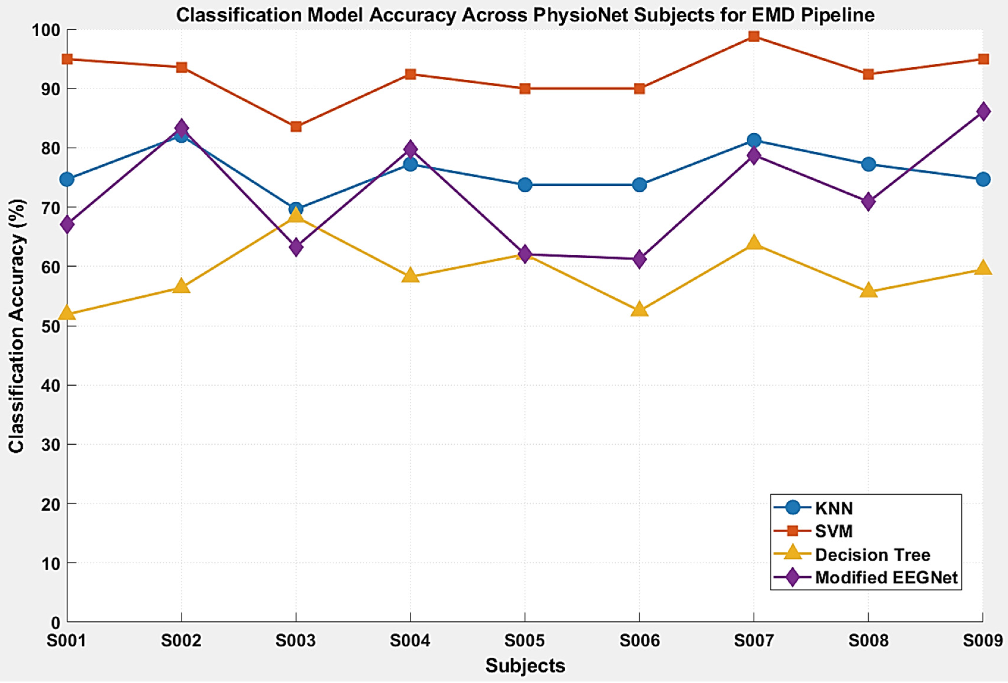
Under the EMD configuration (Figure 14,

Table 20. Comparative classification accuracy across multiple architectures for EMD pipeline in PhysioNet subset.

	S001	S002	S003	S004	S005	S006	S007	S008	S009	Average
KNN	74.68%	82.05%	69.62%	77.22%	77.22%	73.75%	81.25%	77.22%	74.68%	76.41% ± 3.60%
SVM	94.94%	93.59%	83.54%	92.41%	93.67%	90.00%	98.75%	92.41%	94.94%	92.69% ± 3.94%
Decision Tree	51.90%	56.41%	68.35%	58.23%	60.76%	52.50%	63.75%	55.70%	59.49%	58.56% ± 4.97%
Modified EEGNet	67.09%	83.33%	63.29%	79.75%	62.03%	61.25%	78.75%	70.89%	86.08%	72.50% ± 9.11%

), the pipeline mitigates non-stationary components to deliver consistent tracking across the cohort. High-proficiency users anchor performance, with S007 achieving the highest SVM accuracy. The decomposition stabilizes the KNN performance, yielding a marked improvement over baseline levels. Subject-level analysis demonstrates how EMD mitigates low SNR constraints. For instance, S006, who struggled in previous configurations, shows a substantial recovery in KNN and SVM accuracy. By isolating physical signal modes, EMD exposes faint MI rhythms previously masked by background noise, allowing the SVM to maintain high-tier performance even when simpler models remain limited by subtle signal traits.

However, EMD’s non-linear unmixing introduces specific architectural vulnerabilities. A performance inversion occurs in S003, where the EMD-processed temporal distributions favor threshold-based models while disrupting the clear boundaries required by maximum-margin hyperplanes and convolutional layers. Similarly, S005 highlights a deep learning blindspot: despite robust SVM and KNN results, modified EEGNet accuracy collapses. This indicates that resulting IMFs can introduce temporal jitter or phase irregularities that confuse convolutional filters, contributing to higher variability within deep learning architectures.

To ensure stability, the Adaptive Laplacian filter mitigates broadband noise before EMD processing. This pre-cleared spatial foundation allows EMD to operate under a constrained two-iteration limit, providing necessary data-driven unmixing without distorting the underlying signal. As a result, the subsequent adaptive WPD stage creates a highly optimized feature extraction environment. By extracting features from these spatially pre-conditioned signals rather than raw bandpass-filtered data, the pipeline ensures the resulting feature vectors capture pure, unmixed MI rhythms, leading to significant accuracy gains for challenging subjects and stabilizing cohort-wide performance.

The diagonal cluster of hit-rates across all four MI classes demonstrates that the adaptive WPD architecture reliably captures complex multi-limb intentions without skewing toward specific target tasks. Furthermore, the top-performing subject profile from each pipeline is highlighted to establish the framework’s potential performance ceiling and to demonstrate its capacity to resolve complex class boundaries under optimal conditions, as shown in Figure 15. Within the No-BSS baseline pipeline in Figure 15a, Subject S001 establishes an impressive baseline foundation of 93.67%, proving the system’s inherent ability to resolve distinct class boundaries even when operating with no BSS. For a separate individual under the ICA pipeline in Figure 15b, Subject S009 attains a near-flawless 97.44% accuracy, providing proof that removing transient ocular and muscle artifacts via independent source separation uncovers cognitive signatures, yielding perfect 100% true-positive rates for three out of the four evaluated tasks. The maximum performance ceiling of the entire study is established under the EMD pipeline in Figure 15c by Subject S007, with a peak tracking accuracy of 98.75%. This exceptional profile validates the localized sifting mechanics: by breaking down the non-stationary EEG into distinct intrinsic modes, the EMD pipeline concentrates the sensorimotor rhythm power. This allows the GA to compress the subject’s features down to a compact subset where the SVM hyperplane constructs completely unambiguous class margins across all MI classes.

To systematically evaluate reliability, this study analyzed Cohen’s Kappa, F1-score, Recall, Precision, and AUC across the PhysioNet cohort (

Table 21. Average performance metrics for KNN in PhysioNet subset.

Performance Metrics	No BSS	ICA	EMD
Kappa	0.5448 ± 0.0579	0.5939 ± 0.0653	0.7186 ± 0.0721
F1-Score	0.6594 ± 0.0556	0.6938 ± 0.0495	0.7633 ± 0.0368
Recall	0.6584 ± 0.0573	0.6949 ± 0.0499	0.7634 ± 0.0344
Precision	0.6770 ± 0.0483	0.7055 ± 0.0470	0.7808 ± 0.0372
AUC	0.8923 ± 0.0326	0.8965 ± 0.0252	0.9313 ± 0.0163

,

Table 22. Average performance metrics for SVM in PhysioNet subset.

Performance Metrics	No BSS	ICA	EMD
Kappa	0.8560 ± 0.0429	0.9097 ± 0.0404	0.9025 ± 0.0525
F1-Score	0.8944 ± 0.0309	0.9267 ± 0.0368	0.9258 ± 0.0396
Recall	0.8940 ± 0.0312	0.9284 ± 0.0359	0.9311 ± 0.0378
Precision	0.9051 ± 0.0271	0.9331 ± 0.0366	0.9258 ± 0.0396
AUC	0.9686 ± 0.0174	0.9815 ± 0.0174	0.9782 ± 0.0197

,

Table 23. Average performance metrics for Decision Tree in PhysioNet subset.

Performance Metrics	No BSS	ICA	EMD
Kappa	0.4642 ± 0.0607	0.4829 ± 0.0919	0.4479 ± 0.0656
F1-Score	0.5955 ± 0.0409	0.6043 ± 0.0712	0.5820 ± 0.0468
Recall	0.5976 ± 0.0428	0.6109 ± 0.0686	0.5856 ± 0.0490
Precision	0.6248 ± 0.0487	0.6468 ± 0.0459	0.6184 ± 0.0404
AUC	0.8218 ± 0.0270	0.8251 ± 0.0515	0.8058 ± 0.0357

and

Table 24. Average performance metrics for modified EEGNet in PhysioNet subset.

Performance Metrics	No BSS	ICA	EMD
Kappa	0.6109 ± 0.1380	0.6927 ± 0.0709	0.6330 ± 0.1216
F1-Score	0.7074 ± 0.1030	0.7696 ± 0.0509	0.7218 ± 0.0951
Recall	0.7076 ± 0.1014	0.7704 ± 0.0527	0.7248 ± 0.0915
Precision	0.7173 ± 0.1014	0.7848 ± 0.0536	0.7378 ± 0.0931
AUC	0.8997 ± 0.0459	0.9154 ± 0.0320	0.9011 ± 0.0454

). The alignment between these metrics confirms a balanced feature space, ensuring predictive parity across MI tasks. The SVM consistently establishes the performance ceiling; starting from a high-performance baseline, the SVM is further enhanced by BSS integration, with ICA yielding optimal results and EMD maintaining high-tier stability. The narrow standard deviations across these metrics confirm that the SVM’s decision hyperplanes remain robust, effectively isolating genuine sensorimotor rhythms rather than over-fitting to session-specific baseline noise. In contrast, the KNN demonstrates a systematic performance inversion, with macro-indicators showing progressive accuracy gains through to the EMD pipeline. The sifting mechanism prevents localized noise from distorting distance metrics, allowing the KNN to form clean, uncorrupted geometric class boundaries. The modified EEGNet exhibits a different sensitivity, benefiting from the spatial unmixing of ICA with marked accuracy improvements, but facing destabilization under EMD, where compressed subsets appear to disrupt decision thresholds and Precision–Recall execution. Finally, the Decision Tree remains architecturally bottlenecked, consistently underperforming with only marginal accuracy fluctuations across all configurations due to its inability to model the complex, overlapping variations in MI signals even when provided with high-quality features. These results validate the flexibility of the pipelines and emphasize the necessity of maximum-margin hyperplanes like the SVM for achieving stable, robust BCI performance.

4.3. Computational Efficiency

An evaluation of the execution latencies reveals three distinct trends governed by preprocessing overhead, training volume, and structural model complexity, as shown in

Table 25. Average inference latency for KNN.

Dataset Pool	No BSS	ICA	EMD
BCI Competition IV Dataset 2A
Training Time (s)	0.1927 ± 0.0775	0.3626 ± 0.2083	0.2250 ± 0.1187
Testing Time (s)	0.0695 ± 0.0147	0.0842 ± 0.0368	0.0697 ± 0.0398
PhysioNet
Training Time (s)	0.2477 ± 0.1852	0.1800 ± 0.0599	0.4136 ± 0.2129
Testing Time (s)	0.0792 ± 0.0444	0.0766 ± 0.0252	0.1482 ± 0.0842

,

Table 26. Average inference latency for SVM.

Dataset Pool	No BSS	ICA	EMD
BCI Competition IV Dataset 2A
Training Time (s)	0.5562 ± 0.1012	0.7455 ± 0.2575	0.6389 ± 0.1739
Testing Time (s)	0.0841 ± 0.0212	0.1104 ± 0.0370	0.0889 ± 0.0209
PhysioNet
Training Time (s)	0.6224 ± 0.2291	0.6373 ± 0.1414	0.9279 ± 0.3123
Testing Time (s)	0.0896 ± 0.0335	0.0906 ± 0.0414	0.1422 ± 0.0585

,

Table 27. Average inference latency for Decision Tree.

Dataset Pool	No BSS	ICA	EMD
BCI Competition IV Dataset 2A
Training Time (s)	0.1599 ± 0.0255	0.2327 ± 0.1242	0.1926 ± 0.0588
Testing Time (s)	0.0154 ± 0.0051	0.0231 ± 0.0188	0.0139 ± 0.0040
PhysioNet
Training Time (s)	0.1720 ± 0.0629	0.1845 ± 0.0433	0.2623 ± 0.0860
Testing Time (s)	0.0152 ± 0.0051	0.0197 ± 0.0053	0.0227 ± 0.0075

and

Table 28. Average inference latency for modified EEGNet.

Dataset Pool	No BSS	ICA	EMD
BCI Competition IV Dataset 2A
Training Time (s)	99.9989 ± 24.7504	137.1620 ± 36.2134	147.3385 ± 104.5006
Testing Time (s)	0.1287 ± 0.0345	0.1430 ± 0.0391	0.1465 ± 0.0272
PhysioNet
Training Time (s)	44.3482 ± 19.9092	35.6024 ± 7.3621	56.3234 ± 21.8473
Testing Time (s)	0.1154 ± 0.0713	0.0991 ± 0.0260	0.1283 ± 0.0433

. First, implementing advanced BSS methods systematically increases offline training overhead. Both EMD and ICA increase data complexity, forcing the classifiers to perform heavier math to find clear decision boundaries.

Second, a training footprint disparity emerges within the deep learning architecture based on dataset scale. Modified EEGNet consistently requires substantially longer optimization times across all pipelines on Dataset 2A compared to PhysioNet. This illustrates that iterative backpropagation overhead scales directly with the higher trial density of the Competition dataset regardless of the preprocessing configuration. The remaining classifiers demonstrate efficient training profiles. Decision Trees and KNN involve minimal computational cost, as the Decision Tree utilizes greedy splitting criteria to organize the data, while the KNN requires only the storage of training vectors rather than iterative optimization. Although SVMs are often considered computationally demanding, the integration of a GA-optimized feature set significantly reduces input dimensionality, ensuring rapid convergence and keeping the training duration under one second. Collectively, these findings demonstrate that the training phase for all models is well within acceptable practical constraints.

Third, real-time online testing inference latencies follow a structural hierarchy across both data pools, with execution speeds increasing from Decision Trees (~15 ms), through the distance matching of KNN (~70–80 ms) and kernel projections of SVM (~80–140 ms), to the multi-layer forward propagation of EEGNet (~100–146 ms). As real-time testing uses fixed mathematical formulas rather than repetitive training loops, even the worst-case configurations run safely below the standard 250–500 ms BCI window update limit.

As a result, the SVM strikes the optimal engineering balance across all configurations. Furthermore, these averages reflect batch-processed testing; the actual inference latency for a single trial in a live operational loop will be lower than the shown results. While these results indicate the pipeline’s potential for real-time application, they do not account for external factors such as signal acquisition, buffering, or communication delays. As a result, these findings establish the computational viability of the classification stage, while future work will be required to validate the full end-to-end system latency.

4.4. Comparative Performance Analysis

The architectural effectiveness of the proposed No-BSS pipeline was evaluated by benchmarking performance against state-of-the-art BSS signal decomposition and denoising techniques. Among the four classification paradigms tested, the SVM consistently demonstrated superior accuracy across both datasets. This model was therefore adopted as the primary classifier to provide a controlled baseline for comparison. It is important to note that the results presented in this section are intended to demonstrate the performance of the proposed framework under specific conditions and are not strictly comparable to existing benchmarks in the literature. Variations in data preprocessing, subject selection criteria, feature engineering, and the specific validation protocols employed across different studies preclude a direct one-to-one performance comparison. For comparative purposes, literature-reported average accuracy values were utilized; however, it should be noted that subject counts for the PhysioNet dataset were not specified in the corresponding BSS-based benchmark [54].

Table 29. Comparative classification accuracy of the proposed No-BSS pipeline and established BSS-based benchmarks.

Methodology	Dataset	Subject Count	Average Accuracy
ICA-WT-CSP [54]	PhysioNet	None Specified	81.75%
DWT-EMD-Approximate Entropy [37]	BCI Competition IV Dataset 2A	9	85.71%
ICA-Wavelet-CSP [55]	BCI Competition IV Dataset 2A	9	82.00%
ORICA-CSP [55]	BCI Competition IV Dataset 2A	9	89.00%
Proposed Pipeline (No-BSS)	PhysioNet	9	89.47%
Proposed Pipeline (No-BSS)	BCI Competition IV Dataset 2A	9	90.28%

presents the classification performance of the proposed No-BSS pipeline, which reaches 89.47% accuracy on the PhysioNet dataset with nine subjects and 90.28% on the BCI Competition IV Dataset 2A. This performance is comparable to, and outperforms, existing BSS-based benchmarks [37,54,55]. While BSS approaches such as ICA-WT-CSP and DWT-EMD are recognized as established methods, they often require global signal decomposition, which can introduce computational complexity and reliance on heuristic-based parameters. In contrast, these results demonstrate that replacing global BSS decomposition with a subject-adaptive approach achieves equivalent or superior discriminative power. This validates that the proposed adaptive approach effectively isolates neural nodes unique to each subject, providing a distinct advantage: the framework attains high-fidelity classification accuracy while bypassing the reliance on the universal BSS-based priors characteristic of traditional methodologies.

5. Discussion

The experimental findings demonstrate that the proposed architectural configurations counter the prominent challenges of low SNR, session-to-session variability, and data scarcity inherent to MI-BCIs. Across the three developed pipelines, the integration of BSS and an Adaptive Laplacian filter isolates true neural intent from severe physiological artifacts, boosting the raw SNR. The application of BSS proved foundational to the downstream feature extraction. By isolating and removing ocular and muscular artifacts prior to decomposition, it prevented the classifiers from learning non-cerebral noise pathways, which directly stabilized the feature spaces of weaker models. To mitigate session-to-session and subject-to-subject non-stationarity, the subject-specific WPD combined with a Fisher Score ensures that the system avoids rigid, universal frequency boundaries. Instead, it dynamically isolates and ranks the specific time-frequency nodes exhibiting the highest discriminative power of the MI classes for each individual user. Confining this extraction strictly to channels C3, C4, and Cz targets the primary sensorimotor regions directly associated with MI, capturing essential spatial-temporal-frequency profiles of Event-Related Desynchronization (ERD) and Event-Related Synchronization (ERS) while eliminating the computational strain of full-scalp configurations.

The subsequent feature pruning and classification stages underscore how mitigating the curse of dimensionality and data scarcity stabilizes performance across the pipelines. Out of the initial pool of 36 features, the GA functions as a global evolutionary search mechanism to filter out redundant or highly correlated features. To address data scarcity, a Gaussian data augmentation strategy was implemented across the datasets. The results confirm the augmentation did not overwhelm the underlying neural patterns or trigger synthetic data leakage.

As the feature selection via adaptive WPD was strictly tuned to individual subject characteristics, a clear performance hierarchy emerged across the classifiers. Rather than yielding universally inflated accuracies, the models exhibited realistic, data-driven distributions: the SVM established a highly reliable maximum-margin decision boundary to lead performance, followed by KNN, while the modified EEGNet and Decision Tree pipelines lagged behind. This exact hierarchy and distribution held true across both Dataset 2A (with the Decision Tree reflecting baseline constraints in the 30% to 50% range) and the PhysioNet subset of nine subjects (ranging from 30% to 60%). This consistent performance trend across both datasets suggests the pipelines extract genuine neural features, avoiding the pitfalls of artificial shortcut learning.

Two-tailed paired t-tests were employed to evaluate the performance stability of the proposed architecture. The analysis revealed the No-BSS pipeline achieves performance levels comparable to the BSS-equipped pipelines, with only isolated instances of statistically significant variance ($p<0.05$). This suggests the proposed framework serves as a high-efficiency alternative, maintaining classification accuracy while reducing the computational burden associated with traditional BSS-based processing.

As a result, evaluating these three distinct pipelines reveals an optimized engineering balance between algorithmic complexity and real-world execution viability. While training complex architectures demands a heavier computational footprint during offline calibration, the live online inference phase for all three models scales down to straightforward, single-trial vector operations. As the real-time loop completely bypasses iterative optimization routines, the operational latency for individual model predictions drops significantly below offline averages. This provides a substantial processing safety margin relative to the 250–500 ms real-time constraint, indicating that these localized processing pipelines are computationally viable for potential hardware-in-the-loop implementation. Future testing will be required to validate end-to-end performance within a complete hardware–software signal chain.

A notable limitation of this evaluation involves the computational complexity introduced by the GA during feature selection. Although the pipeline is engineered for low-latency, real-time performance, the GA operates as an intensive, iterative process requiring approximately 5 min for convergence per subject. Within practical neuro-rehabilitation settings, this computational bottleneck can be mitigated by confining the GA to an offline, pre-session calibration phase. This step can be designed to occur during routine clinical preparation, such as when a therapist fits the localized electrode array (C3, C4, Cz, and neighboring channels) or stabilizes a patient within a robotic lower-limb exoskeleton. Constraining the GA search space to a bounded 36-feature matrix ensures rapid optimization convergence before the algorithm terminates and exports a static feature mask to the live system. Alternatively, to eliminate pre-session initialization delays in high-throughput clinical workflows, a deterministic iterative Relief-F wrapper can substitute for the GA. This approach utilizes Relief-F to rank the 36 localized features by class discriminability in a single step, followed by a sequential forward selection loop that incrementally adds the ranked features to a classifier until peak accuracy is reached. Because this deterministic execution completes in milliseconds rather than minutes, the iterative Relief-F wrapper maintains the multi-class feature evaluation capabilities of the original architecture while removing initialization latency. This alternative provides a plug-and-play configuration, enabling assistive rehabilitation hardware to trigger synchronously with the patient’s immediate neural intent from the onset of the session to support neuroplastic recovery.

Another limitation of this study is the absence of a stage-by-stage ablation analysis to understand the individual contribution of every algorithmic component. However, the study is structured as a comparative ablation study of BSS paradigms. By evaluating three distinct pipelines, this research demonstrates that the No-BSS pipeline achieves performance comparable to the BSS-optimized approaches.

A final limitation is that evaluation was conducted entirely within an intra-subject framework, and a comprehensive cross-subject analysis was not performed. While the current validation protocol utilizes a 70/30 intra-session hold-out to prevent data leakage, it does not account for the non-stationary distribution shifts associated with multi-session or inter-session BCI usage. This was a deliberate design choice dictated by the pipeline’s underlying mathematical architecture, which is engineered to adapt dynamically to individual physiological differences rather than generalize across a population. As the combination of a local Laplacian spatial filter and adaptive WPD nodes is tailored to mitigate session-to-session and subject-to-subject non-stationarity, the resulting feature masks are effectively optimized for each participant’s unique signal characteristics. MI features may exhibit significant inter-subject variability, which is often attributed to potential physiological and cognitive factors, such as skull thickness, cortical folding, and individual MI strategies. As a result, a cross-subject transfer paradigm would fundamentally conflict with the subject-specific optimization strategy that enables the low-latency pipeline to achieve high classification accuracy. While the structural stability of the performance hierarchy was successfully validated across two independent, standard benchmarks, evaluating the generalizability of these static feature masks to completely novel, subject-independent clinical paradigms remains a task for future adaptive transfer learning research using domain adaptation.

6. Conclusions

This study investigated the operational balance between algorithmic complexity and execution latency in four-class MI-BCIs by validating three localized pipelines on the BCI Competition IV Dataset 2A and the PhysioNet MI datasets. Utilizing an Adaptive Laplacian spatial filter localized to channels C3, C4, and Cz, paired with a subject-specific WPD and Fisher Score selection scheme, the system successfully extracted true neural patterns from nodes and countered non-stationarity without full-scalp computational strain. Additionally, a Gaussian noise injection technique effectively increased sample density to safeguard against poor classification boundaries across the data pools. The experimental results demonstrated a highly stable performance hierarchy, with the ICA pipeline achieving top accuracy, followed in order by the EMD configuration and the lightweight pipeline without BSS. Within these pipelines, a consistent model distribution emerged: the SVM achieved the highest performance by establishing a maximum-margin decision boundary over the 36-feature space optimized by a GA, followed sequentially by KNN, a modified EEGNet, and Decision Trees. The No-BSS baseline yielded classification accuracies competitive with the BSS-dependent pipelines while completely avoiding their intensive runtime processing delays, proving its value as a highly efficient alternative for time-sensitive, live BCI control loops. To enable a high-throughput, live-adaptive clinical tool, future work will replace the GA with a deterministic, iterative Relief-F wrapper to achieve millisecond-scale feature mask initialization. Future work will incorporate $k$-fold cross-validation to more robustly assess model stability, addressing the limitations of the current fixed train-test split. Future work will explore cross-subject transfer learning to improve generalizability across diverse population profiles. Validation on independent datasets will ensure framework robustness beyond established benchmarks. Subsequent development will focus on live, real-time BCI implementation to evaluate performance under dynamic conditions. These efforts will establish a scalable, low-latency processing blueprint capable of triggering assistive rehabilitation hardware in synchrony with neural intent.

References

1. Mdluli, B.; Khumalo, P.; Maswanganyi, R.C. Signal Preprocessing, Decomposition and Feature Extraction Methods in EEG-Based BCIs. Appl. Sci. 2025, 15, 12075. [Google Scholar] [CrossRef] [Scilit]
2. Ramsoonder, N.; Maswanganyi, R.C.; Khumalo, P. Comparative Performance Analysis of Machine Learning Computational Pipelines and Deep Learning Architectures in EEG Motor Imagery BCIs. Mathematics 2026, 14, 1520. [Google Scholar] [CrossRef] [Scilit]
3. Maswanganyi, R.C.; Tu, C.; Owolawi, P.A.; Du, S. Statistical Evaluation of Factors Influencing Inter-Session and Inter-Subject Variability in EEG-Based Brain Computer Interface. IEEE Access 2022, 10, 96821–96839. [Google Scholar] [CrossRef] [Scilit]
4. Molla, M.K.I.; Al Shiam, A.; Islam, M.R.; Tanaka, T. Discriminative Feature Selection-Based Motor Imagery Classification Using EEG Signal. IEEE Access 2020, 8, 98255–98265. [Google Scholar] [CrossRef] [Scilit]
5. Singh, A.; Hussain, A.A.; Lal, S.; Guesgen, H.W. A Comprehensive Review on Critical Issues and Possible Solutions of Motor Imagery Based Electroencephalography Brain–Computer Interface. Sensors 2021, 21, 2173. [Google Scholar] [CrossRef] [Scilit] [PubMed]
6. Khan, R.A.; Rashid, N.; Shahzaib, M.; Malik, U.F.; Arif, A.; Iqbal, J.; Saleem, M.; Khan, U.S.; Tiwana, M. A Novel Framework for Classification of Two-Class Motor Imagery EEG Signals Using Logistic Regression Classification Algorithm. PLoS ONE 2023, 18, e0276133. [Google Scholar] [CrossRef] [Scilit] [PubMed]
7. Jiang, X.; Bian, G.B.; Tian, Z. Removal of Artifacts from EEG Signals: A Review. Sensors 2019, 19, 987. [Google Scholar] [CrossRef] [Scilit] [PubMed]
8. Mannan, M.M.N.; Kamran, M.A.; Jeong, M.Y. Identification and Removal of Physiological Artifacts from Electroencephalogram Signals: A Review. IEEE Access 2018, 6, 30630–30652. [Google Scholar] [CrossRef] [Scilit]
9. Dhole, P.V.; Chaudhary, D.G.; Dhangar, V.D.; Shejul, S.D.; Datwase, S.S.; Gawali, B.W. A Review of EEG Artifact Removal Techniques for Brain–Computer Interface. SN Comput. Sci. 2025, 6, 1026. [Google Scholar] [CrossRef] [Scilit]
10. Wu, C.; Yao, B.; Zhang, X.; Li, T.; Wang, J.; Pu, J. The Application of Entropy in Motor Imagery Paradigms of Brain–Computer Interfaces. Brain Sci. 2025, 15, 168. [Google Scholar] [CrossRef] [Scilit] [PubMed]
11. Titkanlou, M.K.; Pham, D.T.; Mouček, R. Classification of EEG Signal Using Deep Learning Architectures Based Motor-Imagery for an Upper-Limb Rehabilitation Exoskeleton. SN Comput. Sci. 2025, 6, 193. [Google Scholar] [CrossRef] [Scilit]
12. Sung, D.J.; Kim, K.T.; Jeong, J.H.; Kim, L.; Lee, S.J.; Kim, H.; Kim, S.J. Improving Inter-Session Performance via Relevant Session-Transfer for Multi-Session Motor Imagery Classification. Heliyon 2024, 10, e37343. [Google Scholar] [CrossRef] [Scilit] [PubMed]
13. Amer, N.S.; Belhaouari, B. EEG Signal Processing for Medical Diagnosis, Healthcare, and Monitoring: A Comprehensive Review. IEEE Access 2023, 11, 139457–139465. [Google Scholar] [CrossRef] [Scilit]
14. Shyu, K.K.; Huang, S.C.; Tung, K.J.; Lee, L.H.; Lee, P.L.; Chen, Y.H. Common Spatial Pattern and Riemannian Manifold-Based Real-Time Multiclass Motor Imagery EEG Classification. IEEE Access 2023, 11, 139457–139465. [Google Scholar] [CrossRef] [Scilit]
15. Delorme, A. EEG Is Better Left Alone. Sci. Rep. 2023, 13, 2372. [Google Scholar] [CrossRef] [Scilit] [PubMed]
16. Siviero, I.; Menegaz, G.; Storti, S.F. Functional Connectivity and Feature Fusion Enhance Multiclass Motor-Imagery Brain–Computer Interface Performance. Sensors 2023, 23, 7520. [Google Scholar] [CrossRef] [Scilit] [PubMed]
17. Velasco, I.; Sipols, A.; De Blas, C.S.; Pastor, L.; Bayona, S. Motor Imagery EEG Signal Classification with a Multivariate Time Series Approach. Biomed. Eng. Online 2023, 22, 29. [Google Scholar] [CrossRef] [Scilit] [PubMed]
18. Yan, Y.; Zhou, H.; Huang, L.; Cheng, X.; Kuang, S. A Novel Two-Stage Refine Filtering Method for EEG-Based Motor Imagery Classification. Front. Neurosci. 2021, 15, 657540. [Google Scholar] [CrossRef] [Scilit] [PubMed]
19. Zhang, Z.; Duan, F.; Sole-Casals, J.; Dinares-Ferran, J.; Cichocki, A.; Yang, Z.; Sun, Z. A Novel Deep Learning Approach with Data Augmentation to Classify Motor Imagery Signals. IEEE Access 2019, 7, 15945–15954. [Google Scholar] [CrossRef] [Scilit]
20. Sharma, N.; Sharma, M.; Singhal, A.; Vyas, R.; Malik, H.; Hossaini, M.A.; Afthanorhan, A. An Efficient Approach for Recognition of Motor Imagery EEG Signals Using the Fourier Decomposition Method. IEEE Access 2023, 11, 122782–122791. [Google Scholar] [CrossRef] [Scilit]
21. Li, M.A.; Zhu, W.; Liu, H.N.; Yang, J.F. Adaptive Feature Extraction of Motor Imagery EEG with Optimal Wavelet Packets and SE-Isomap. Appl. Sci. 2017, 7, 390. [Google Scholar] [CrossRef] [Scilit]
22. George, O.; Smith, R.; Madiraju, P.; Yahyasoltani, N.; Ahamed, S.I. Data Augmentation Strategies for EEG-Based Motor Imagery Decoding. Heliyon 2022, 8, e10240. [Google Scholar] [CrossRef] [Scilit] [PubMed]
23. Petrov, M. Optimizing Motor Imagery BCIs: A Motor Imagery EEG Classification Protocol Using Evolutionary Optimization and Low Sample Training-Sets. Master’s Thesis, New College of Florida, Sarasota, FL, USA, 2024. Available online: https://digitalcommons.ncf.edu/theses_etds/6586 (accessed on 15 May 2026).
24. Dhiman, R. Wavelet Packet Decomposition of Electroencephalogram Signals for Brain Computer Interface. Available online: https://aeteps2023.wordpress.com/wp-content/uploads/2023/06/aeteps2023_id_278.pdf (accessed on 15 May 2026).
25. Geng, X.; Wang, L.; Yu, P.; Hu, W.; Liang, Q.; Zhang, X.; Chen, C.; Zhang, X. A Method of EEG Signal Feature Extraction Based on Hybrid DWT and EMD. Alex. Eng. J. 2025, 113, 195–204. [Google Scholar] [CrossRef] [Scilit]
26. Kabir, M.H.; Akhtar, N.I.; Tasnim, N.; Miah, A.S.M.; Lee, H.S.; Jang, S.W.; Shin, J. Exploring Feature Selection and Classification Techniques to Improve the Performance of an Electroencephalography-Based Motor Imagery Brain–Computer Interface System. Sensors 2024, 24, 4989. [Google Scholar] [CrossRef] [Scilit] [PubMed]
27. BCI Competition IV. Available online: https://www.bbci.de/competition/iv/ (accessed on 10 July 2026).
28. Schalk, G.; McFarland, D.J.; Hinterberger, T.; Birbaumer, N.; Wolpaw, J.R. EEG Motor Movement/Imagery Dataset. PhysioNet, 2009. Available online: https://physionet.org/content/eegmmidb/1.0.0/ (accessed on 25 April 2026).
29. Savadi, S. A Comprehensive Review of Feature Extraction and Classification Techniques in EEG Signal Analysis. Int. J. Comput. Eng. Res. 2025, 15, 51–62. Available online: http://www.ijceronline.com (accessed on 10 May 2026).
30. Bahhah, M.A.; Attar, E.T. Enhancing Epilepsy Seizure Detection Through Advanced EEG Preprocessing Techniques and Peak-to-Peak Amplitude Fluctuation Analysis. Diagnostics 2024, 14, 2525. [Google Scholar] [CrossRef] [Scilit] [PubMed]
31. Shieh, C.P.; Yang, S.H.; Liu, Y.S.; Kuo, Y.T.; Lo, Y.C.; Kuo, C.H.; Chen, Y.Y. Simultaneously Spatiospectral Pattern Learning and Contaminated Trial Pruning for Electroencephalography-Based Brain Computer Interface. Symmetry 2020, 12, 1387. [Google Scholar] [CrossRef] [Scilit]
32. Visu, P.; Smitha, P.S.; Velayutham, M.; Ahmad, M.W. Enhanced EEG Classification Using Adaptive DWT and Heuristic-ICA Algorithm. Automatika 2023, 64, 827–836. [Google Scholar] [CrossRef] [Scilit]
33. Blum, S.; Jacobsen, N.S.J.; Bleichner, M.G.; Debener, S. A Riemannian Modification of Artifact Subspace Reconstruction for EEG Artifact Handling. Front. Hum. Neurosci. 2019, 13, 141. [Google Scholar] [CrossRef] [Scilit] [PubMed]
34. Van Jaarsveldt, C.; Peters, G.W.; Ames, M.; Chantler, M. Tutorial on Empirical Mode Decomposition: Basis Decomposition and Frequency Adaptive Graduation in Non-Stationary Time Series. IEEE Access 2023, 11, 94442–94478. [Google Scholar] [CrossRef] [Scilit]
35. Rabbath, C.A.; Corriveau, D. A Comparison of Piecewise Cubic Hermite Interpolating Polynomials, Cubic Splines and Piecewise Linear Functions for the Approximation of Projectile Aerodynamics. Def. Technol. 2019, 15, 741–757. [Google Scholar] [CrossRef] [Scilit]
36. Wang, F.; Liu, H.; Zhao, L.; Su, L.; Zhou, J.; Gong, A.; Fu, Y. Improved Brain–Computer Interface Signal Recognition Algorithm Based on Few-Channel Motor Imagery. Front. Hum. Neurosci. 2022, 16, 880304. [Google Scholar] [CrossRef] [Scilit] [PubMed]
37. Ji, N.; Ma, L.; Dong, H.; Zhang, X. EEG Signals Feature Extraction Based on DWT and EMD Combined with Approximate Entropy. Brain Sci. 2019, 9, 201. [Google Scholar] [CrossRef] [Scilit] [PubMed]
38. Beniczky, S.; Schomer, D.L. Electroencephalography: Basic Biophysical and Technological Aspects Important for Clinical Applications. Epileptic Disord. 2020, 22, 697–715. [Google Scholar] [CrossRef] [Scilit] [PubMed]
39. Bradshaw, L.A.; Wikswo, J.P. Spatial Filter Approach for Evaluation of the Surface Laplacian of the Electroencephalogram and Magnetoencephalogram. Ann. Biomed. Eng. 2001, 29, 202–213. [Google Scholar] [CrossRef] [Scilit] [PubMed]
40. Gu, Q.; Li, Z.; Han, J. Generalized Fisher Score for Feature Selection. In Proceedings of the Twenty-Seventh Conference on Uncertainty in Artificial Intelligence, Barcelona, Spain, 14–17 July 2011; AUAI Press: Arlington, VA, USA, 2011. [Google Scholar]
41. Degirmenci, M.; Yuce, Y.K.; Perc, M.; Isler, Y. EEG Channel and Feature Investigation in Binary and Multiple Motor Imagery Task Predictions. Front. Hum. Neurosci. 2024, 18, 1525139. [Google Scholar] [CrossRef] [Scilit] [PubMed]
42. Mateen, N.; Naeem, M.; Khan, M.J.; Yousaf, T.; Ali, A.; Altabey, W.A.; Noori, M.; Kouritem, S.A. Subject Based Feature Selection for Hybrid Brain Computer Interface Using Genetic Algorithm and Support Vector Machine. Results Eng. 2025, 27, 105649. [Google Scholar] [CrossRef] [Scilit]
43. Dhiman, R.; Anshul. Brain Computer Interface Using Genetic Algorithm with Modified Genome and Phenotype Structures. J. Inf. Technol. Manag. 2023, 15, 47–68. [Google Scholar] [CrossRef]
44. Konjkav, A.; Jahangiri, F.; Sajedin, A. Classification Algorithms of EEG Signals Based on Motor Imagery. Int. J. Res. Technol. Electr. Ind. 2025, 4, 517–525. [Google Scholar] [CrossRef]
45. Yassine, F.A.; Abdelkader, G. Enhancing EEG-Based Brain–Computer Interface Systems through Efficient Machine Learning Classification Techniques. Indones. J. Electr. Eng. Comput. Sci. 2024, 34, 2045–2054. [Google Scholar] [CrossRef] [Scilit]
46. Chen, M.; Lee, C.; Chun, Y. A Machine Learning Approach Using Spatially Explicit K-Nearest Neighbors for House Price Predictions. ISPRS Int. J. Geo-Inf. 2026, 15, 46. [Google Scholar] [CrossRef] [Scilit]
47. Syriopoulos, P.K.; Kalampalikis, N.G.; Kotsiantis, S.B.; Vrahatis, M.N. KNN Classification: A Review. Ann. Math. Artif. Intell. 2025, 93, 43–75. [Google Scholar] [CrossRef] [Scilit]
48. Lu, Y.; Wang, W.; Lian, B.; He, C. Feature Extraction and Classification of Motor Imagery EEG Signals in Motor Imagery for Sustainable Brain–Computer Interfaces. Sustainability 2024, 16, 6627. [Google Scholar] [CrossRef] [Scilit]
49. Selim, S.; Tantawi, M.M.; Shedeed, H.A.; Badr, A. A CSP\AM-BA-SVM Approach for Motor Imagery BCI System. IEEE Access 2018, 6, 49192–49208. [Google Scholar] [CrossRef] [Scilit]
50. Ferracuti, F.; Iarlori, S.; Mansour, Z.; Monteriù, A.; Porcaro, C. Comparing between Different Sets of Preprocessing, Classifiers, and Channels Selection Techniques to Optimise Motor Imagery Pattern Classification System from EEG Pattern Recognition. Brain Sci. 2022, 12, 57. [Google Scholar] [CrossRef] [Scilit] [PubMed]
51. Deng, X.; Zhang, B.; Yu, N.; Liu, K.; Sun, K. Advanced TSGL-EEGNet for Motor Imagery EEG-Based Brain–Computer Interfaces. IEEE Access 2021, 9, 25118–25130. [Google Scholar] [CrossRef] [Scilit]
52. Mdluli, B.; Khumalo, P.; Maswanganyi, R.C. Subject-Specific Comparative Performance Analysis of Deep Learning Architectures for Motor Imagery Classification. Mathematics 2026, 14, 1527. [Google Scholar] [CrossRef] [Scilit]
53. Xie, Y.; Oniga, S. Classification of Motor Imagery EEG Signals Based on Data Augmentation and Convolutional Neural Networks. Sensors 2023, 23, 1932. [Google Scholar] [CrossRef] [Scilit] [PubMed]
54. Geng, X.; Li, D.; Chen, H.; Yu, P.; Yan, H.; Yue, M. An Improved Feature Extraction Algorithms of EEG Signals Based on Motor Imagery Brain–Computer Interface. Alex. Eng. J. 2022, 61, 4807–4820. [Google Scholar] [CrossRef] [Scilit]
55. Antony, M.J.; Sankaralingam, B.P.; Mahendran, R.K.; Gardezi, A.A.; Shafiq, M.; Choi, J.G.; Hamam, H. Classification of EEG Using Adaptive SVM Classifier with CSP and Online Recursive Independent Component Analysis. Sensors 2022, 22, 7596. [Google Scholar] [CrossRef] [Scilit] [PubMed]
Figure 1. (a) Pipeline A—No BSS, (b) Pipeline B—ICA, (c) Pipeline C—EMD.
Bdcc 10 00280 g001
Figure 2. Timing paradigm for BCI Competition IV Dataset 2A [27].
Bdcc 10 00280 g002
Figure 3. ICA decision logic for artifact rejection and component retention. Green paths indicate automated and manual acceptance, while red paths denote noise-based or physiological rejection.
Bdcc 10 00280 g003
Figure 4. Adaptive WPD feature extraction logic. Flowchart detailing the multi-stage filtering and ranking process used to mitigate session-to-session variability through subject-specific node selection.
Bdcc 10 00280 g004
Figure 6. Average classification accuracies of the evaluated processing pipelines and classifier architectures on the BCI Competition IV Dataset 2A, illustrating the performance stratification between BSS-free and BSS-dependent configurations.
Bdcc 10 00280 g006
Figure 7. Subject-specific classification accuracy profiles for the No-BSS framework from BCI Competition IV Dataset 2A.
Bdcc 10 00280 g007
Figure 8. Subject-specific classification accuracy profiles for the ICA pipeline from BCI Competition IV Dataset 2A.
Bdcc 10 00280 g008
Figure 9. Subject-specific classification accuracy profiles for the EMD pipeline from BCI Competition IV Dataset 2A.
Bdcc 10 00280 g009
Figure 10. Confusion matrices for best-performing model within-subject configurations in Dataset 2A: (a) Subject A09 under No-BSS baseline, (b) Subject A03 under ICA, and (c) Subject A06 under EMD.
Bdcc 10 00280 g010
Figure 11. Average classification accuracies of the evaluated processing pipelines and classifier architectures on the PhysioNet dataset, illustrating performance trends across BSS-free and BSS-dependent configurations.
Bdcc 10 00280 g011
Figure 12. Subject-specific classification accuracy profiles for the No-BSS pipeline from PhysioNet.
Bdcc 10 00280 g012
Figure 13. Subject-specific classification accuracy profiles for the ICA pipeline from PhysioNet.
Bdcc 10 00280 g013
Figure 14. Subject-specific classification accuracy profiles for the EMD pipeline from PhysioNet.
Bdcc 10 00280 g014
Figure 15. Confusion matrices for best-performing model within-subject configurations in PhysioNet: (a) Subject S001 under No-BSS Baseline, (b) Subject S009 under ICA, and (c) Subject S007 under EMD.
Bdcc 10 00280 g015