Figure 1.
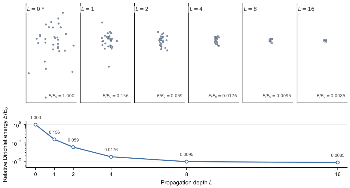
Fixed Gaussian node signals contract under repeated normalized graph diffusion on the Karate Club graph. All projections share one basis and identical axis limits; the lower panel reports relative Dirichlet energy .
Figure 1.
Fixed Gaussian node signals contract under repeated normalized graph diffusion on the Karate Club graph. All projections share one basis and identical axis limits; the lower panel reports relative Dirichlet energy .
Figure 2.
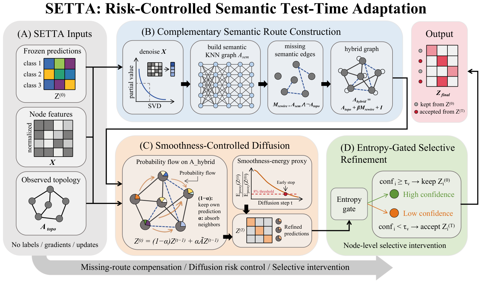
The SETTA framework. SETTA performs prediction-level graph test-time adaptation over frozen GNN predictions without learnable adaptation parameters during refinement. It couples complementary semantic route construction, smoothness-controlled diffusion, and entropy-gated selective refinement. The final output is selected node-wise from the original prediction and the refined prediction .
Figure 2.
The SETTA framework. SETTA performs prediction-level graph test-time adaptation over frozen GNN predictions without learnable adaptation parameters during refinement. It couples complementary semantic route construction, smoothness-controlled diffusion, and entropy-gated selective refinement. The final output is selected node-wise from the original prediction and the refined prediction .
Figure 3.
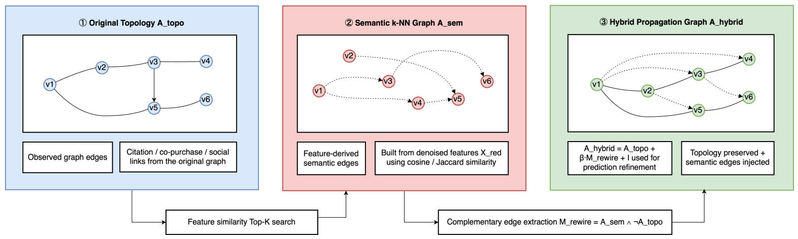
Topology-semantic complementary edge injection. Original topological edges are preserved, feature-aligned semantic neighbors are identified, and only semantic edges absent from the original topology are injected into the hybrid propagation graph.
Figure 3.
Topology-semantic complementary edge injection. Original topological edges are preserved, feature-aligned semantic neighbors are identified, and only semantic edges absent from the original topology are injected into the hybrid propagation graph.
Figure 4.
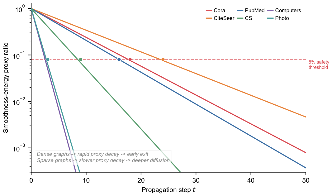
Row-normalized smoothness-energy proxy decay curves across six benchmark datasets. Densely connected graphs dissipate energy rapidly, whereas sparse citation graphs decay more gradually. The 8% threshold provides an adaptive stopping signal during deep propagation.
Figure 4.
Row-normalized smoothness-energy proxy decay curves across six benchmark datasets. Densely connected graphs dissipate energy rapidly, whereas sparse citation graphs decay more gradually. The 8% threshold provides an adaptive stopping signal during deep propagation.
Figure 5.
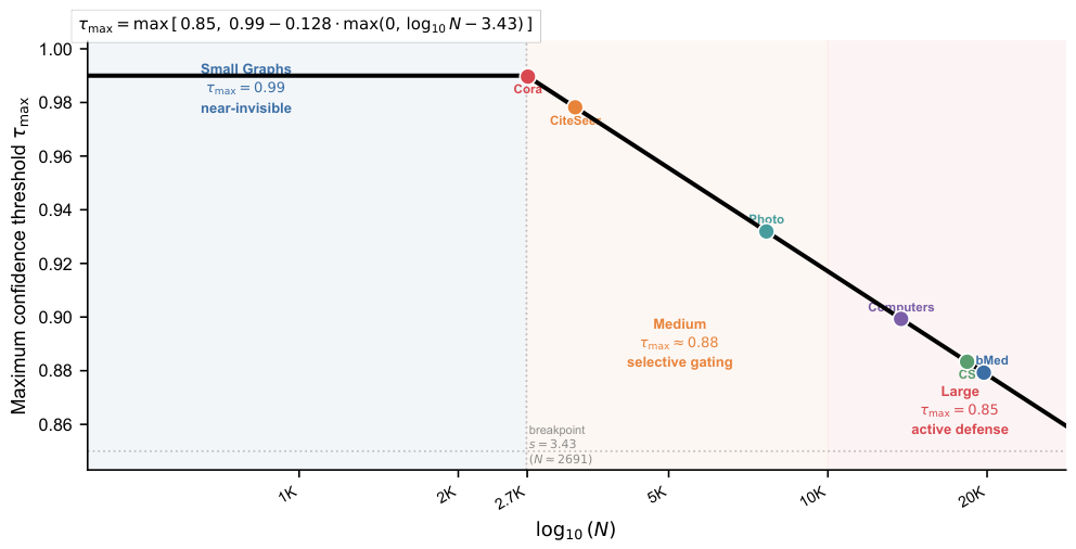
Scale-adaptive maximum confidence threshold. The maximum threshold decreases with graph size until reaching a floor of 0.85, making refinement acceptance more selective on larger graphs.
Figure 5.
Scale-adaptive maximum confidence threshold. The maximum threshold decreases with graph size until reaching a floor of 0.85, making refinement acceptance more selective on larger graphs.
Figure 6.
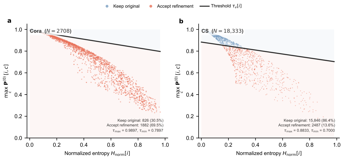
Per-node entropy-gating decision boundaries: (a) Cora, with refinement acceptance dominant; (b) Coauthor-CS, with retention of the original prediction dominant. In both panels, nodes below the threshold curve accept the refined prediction, whereas nodes above it retain the original GCN prediction.
Figure 6.
Per-node entropy-gating decision boundaries: (a) Cora, with refinement acceptance dominant; (b) Coauthor-CS, with retention of the original prediction dominant. In both panels, nodes below the threshold curve accept the refined prediction, whereas nodes above it retain the original GCN prediction.
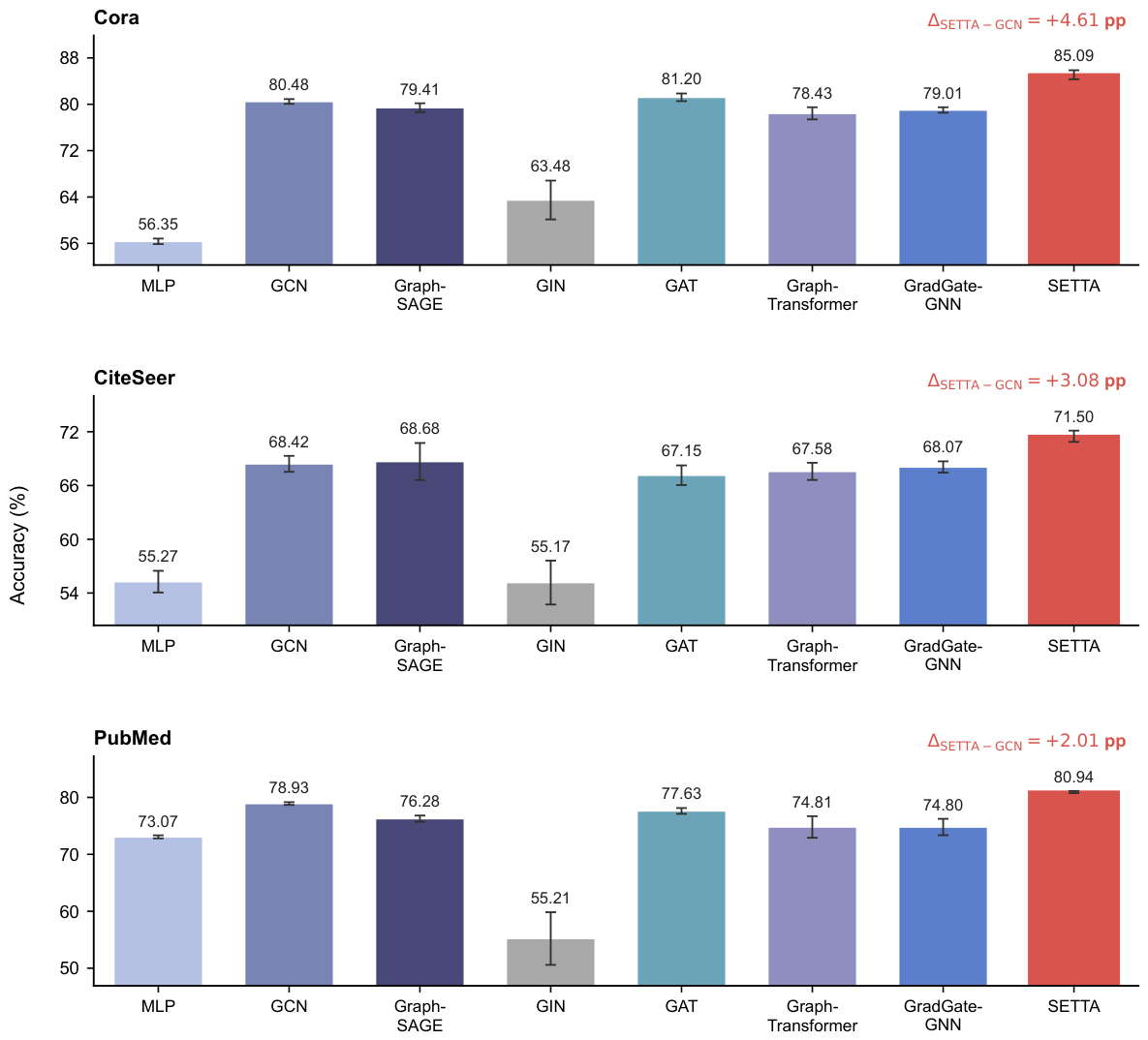
Figure 7.
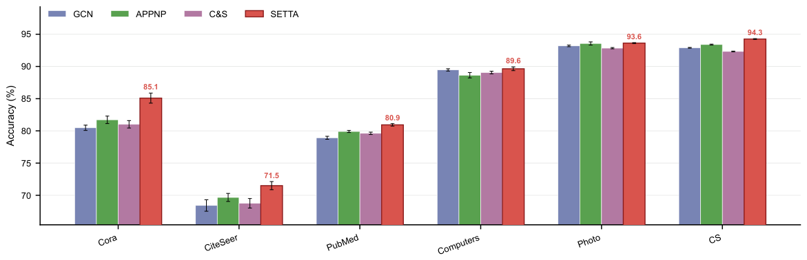
Main results on citation networks under validation-selected SETTA configurations. SETTA achieves the highest mean accuracy among the evaluated methods on Cora, CiteSeer, and PubMed.
Figure 7.
Main results on citation networks under validation-selected SETTA configurations. SETTA achieves the highest mean accuracy among the evaluated methods on Cora, CiteSeer, and PubMed.
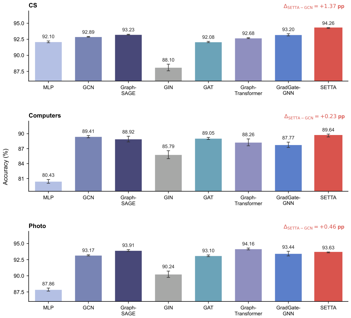
Figure 8.
Results on larger benchmark graphs under validation-selected SETTA configurations. SETTA ranks first among evaluated methods on Coauthor-CS and Amazon-Computers, while GraphTransformer obtains the highest mean accuracy on Amazon-Photo.
Figure 8.
Results on larger benchmark graphs under validation-selected SETTA configurations. SETTA ranks first among evaluated methods on Coauthor-CS and Amazon-Computers, while GraphTransformer obtains the highest mean accuracy on Amazon-Photo.
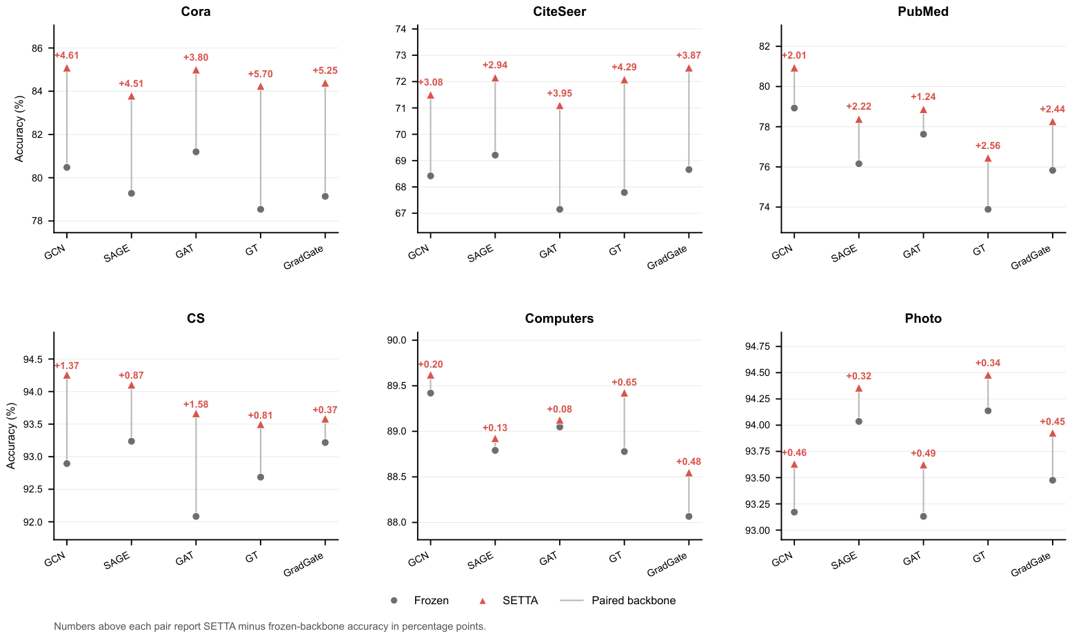
Figure 9.
Backbone-agnostic SETTA refinement on frozen predictions. Each panel compares frozen and SETTA-refined accuracy within one dataset across five frozen GNN backbones. The same dataset-level refinement protocol is used across all backbones without backbone-specific tuning. Numbers above paired points report SETTA accuracy minus frozen-backbone accuracy in percentage points.
Figure 9.
Backbone-agnostic SETTA refinement on frozen predictions. Each panel compares frozen and SETTA-refined accuracy within one dataset across five frozen GNN backbones. The same dataset-level refinement protocol is used across all backbones without backbone-specific tuning. Numbers above paired points report SETTA accuracy minus frozen-backbone accuracy in percentage points.
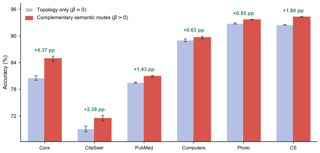
Figure 10.
Semantic edge-injection ablation. Complementary semantic route injection improves over topology-only propagation across all evaluated datasets.
Figure 10.
Semantic edge-injection ablation. Complementary semantic route injection improves over topology-only propagation across all evaluated datasets.
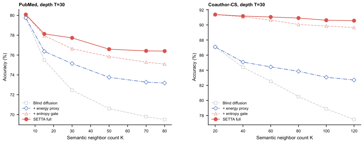
Figure 11.
Dual-defense ablation under deep propagation. Points show the mean accuracies reported in
Table 9. Blind diffusion degrades as the semantic neighbor count increases, while entropy gating and the full SETTA pipeline preserve accuracy more effectively.
Figure 11.
Dual-defense ablation under deep propagation. Points show the mean accuracies reported in
Table 9. Blind diffusion degrades as the semantic neighbor count increases, while entropy gating and the full SETTA pipeline preserve accuracy more effectively.
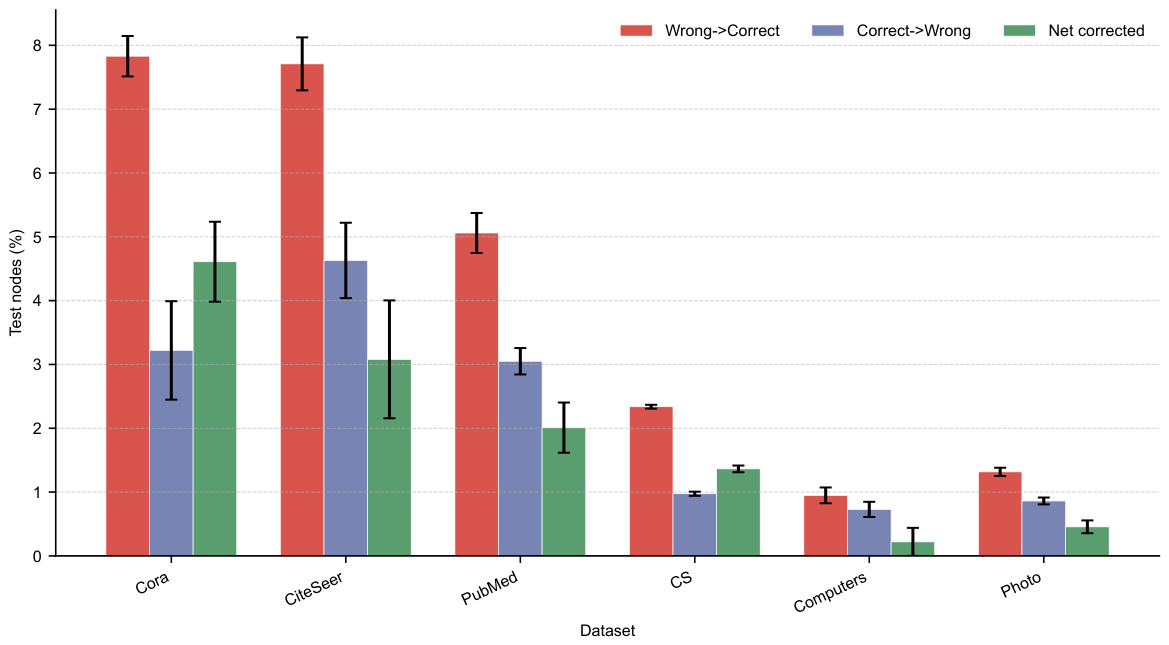
Figure 12.
Node-level transition rates before and after SETTA refinement. Wrong→Correct denotes test nodes incorrectly classified by the frozen GCN but correctly classified after SETTA. Correct→Wrong denotes originally correct predictions changed to incorrect ones. Net correction is computed as Wrong→Correct minus Correct→Wrong. Bars show means over 10 random seeds, and error bars indicate sample standard deviation; they are not confidence intervals. SETTA produces positive net correction on all six datasets.
Figure 12.
Node-level transition rates before and after SETTA refinement. Wrong→Correct denotes test nodes incorrectly classified by the frozen GCN but correctly classified after SETTA. Correct→Wrong denotes originally correct predictions changed to incorrect ones. Net correction is computed as Wrong→Correct minus Correct→Wrong. Bars show means over 10 random seeds, and error bars indicate sample standard deviation; they are not confidence intervals. SETTA produces positive net correction on all six datasets.
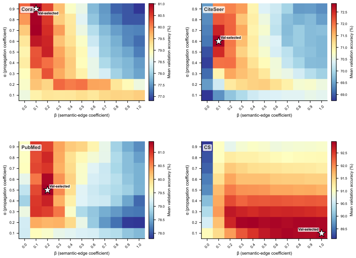
Figure 15.
Validation-based – sensitivity heatmaps on multi-step refinement datasets. Colors indicate mean validation accuracy over 10 seeds. The marked points denote the validation-selected configuration used for final test evaluation. These heatmaps are reported to characterize configuration sensitivity and are not used as test-set selection grids.
Figure 15.
Validation-based – sensitivity heatmaps on multi-step refinement datasets. Colors indicate mean validation accuracy over 10 seeds. The marked points denote the validation-selected configuration used for final test evaluation. These heatmaps are reported to characterize configuration sensitivity and are not used as test-set selection grids.
Figure 16.
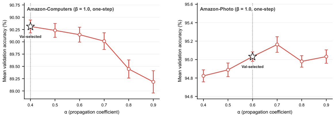
Validation-based sensitivity under the constrained one-step refinement protocol. For Amazon-Computers and Amazon-Photo, is fixed to 1.0 and is selected from the active shallow-refinement range. The star and vertical dotted line in each panel mark the validation-selected used for final test evaluation.
Figure 16.
Validation-based sensitivity under the constrained one-step refinement protocol. For Amazon-Computers and Amazon-Photo, is fixed to 1.0 and is selected from the active shallow-refinement range. The star and vertical dotted line in each panel mark the validation-selected used for final test evaluation.
Table 1.
Method-level comparison under frozen-deployment constraints. “Frozen pred.” indicates whether a method can directly refine an arbitrary prediction matrix without retraining its source model. “Adapt. state” indicates whether parameters, model state, or test-time variables are learned or updated for adaptation.
Table 1.
Method-level comparison under frozen-deployment constraints. “Frozen pred.” indicates whether a method can directly refine an arbitrary prediction matrix without retraining its source model. “Adapt. state” indicates whether parameters, model state, or test-time variables are learned or updated for adaptation.
| Method | Labels in Refinement | Grad./Model Update | Frozen Pred. | Topology | Adapt. State | Semantic Routes | Risk Control |
|---|
| APPNP [15] | No | No | Partial | Preserve | None | No | Restart |
| SGC/SIGN [17,22] | No | Training required | No | Precompute | Predictor | No | Fixed depth |
| C&S [18] | Yes | No | Yes | Preserve | None | No | Label correction |
| GDC [16] | No | Training required | No | Replace operator | None | No | Sparsification |
| GSL/rewiring [20,23,24] | Varies | Usually | Usually no | Modify/replace | Often | Varies | Structural objective |
| TENT [30] | No | Yes | No | Preserve | Updated | No | Entropy objective |
| GraphTTA [31] | No | Yes | No | Augment | Updated | No | Contrastive objective |
| GTrans [32] | No | Yes | No | Transform | Optimized | Varies | Transform objective |
| GT3 [33] | No | Yes | No | Preserve | Updated | No | Self-supervision |
|
SETTA
| No | No | Yes | Preserve + add | None | Yes | Energy + entropy |
Table 2.
SETTA configuration per dataset. K, propagation depth, and similarity metric are fixed by the dataset-level protocol. and are selected using validation data only. For one-step refinement datasets, is fixed to 1.0 and is selected from the active shallow-refinement range . The test split is used only for final evaluation.
Table 2.
SETTA configuration per dataset. K, propagation depth, and similarity metric are fixed by the dataset-level protocol. and are selected using validation data only. For one-step refinement datasets, is fixed to 1.0 and is selected from the active shallow-refinement range . The test split is used only for final evaluation.
| Dataset | | | K | Steps | Metric | | |
|---|
| Cora | 0.9 | 0.1 | 18 | 10 | Jaccard | – | 0.990 |
| CiteSeer | 0.6 | 0.1 | 12 | 10 | Jaccard | – | 0.978 |
| PubMed | 0.5 | 0.2 | 5 | 10 | Cosine | 128 | 0.879 |
| CS | 0.1 | 1.0 | 20 | 10 | Cosine | 850 | 0.883 |
| Computers | 0.4 | 1.0 | 25 | 1 | Cosine | 128 | 0.899 |
| Photo | 0.6 | 1.0 | 30 | 1 | Cosine | 128 | 0.932 |
Table 3.
Node classification accuracy (%) on citation networks. Mean ± standard deviation over 10 random seeds. Best result is represented in bold.
Table 3.
Node classification accuracy (%) on citation networks. Mean ± standard deviation over 10 random seeds. Best result is represented in bold.
| Method | Cora | CiteSeer | PubMed |
|---|
| MLP | 56.35 ± 0.48 | 55.27 ± 1.21 | 73.07 ± 0.27 |
| GCN | 80.48 ± 0.41 | 68.42 ± 0.89 | 78.93 ± 0.24 |
| GraphSAGE | 79.41 ± 0.76 | 68.68 ± 2.07 | 76.28 ± 0.54 |
| GIN | 63.48 ± 3.35 | 55.17 ± 2.45 | 55.21 ± 4.63 |
| GAT | 81.20 ± 0.66 | 67.15 ± 1.10 | 77.63 ± 0.51 |
| GraphTransformer | 78.43 ± 1.05 | 67.58 ± 0.96 | 74.81 ± 1.89 |
| GradGateGNN | 79.01 ± 0.47 | 68.07 ± 0.63 | 74.80 ± 1.44 |
| SETTA (Ours) | 85.09 ± 0.78 | 71.50 ± 0.63 | 80.94 ± 0.19 |
| +4.61 | +3.08 | +2.01 |
Table 4.
Node classification accuracy (%) on larger benchmark datasets. Mean ± standard deviation over 10 random seeds. Best result is represented in bold.
Table 4.
Node classification accuracy (%) on larger benchmark datasets. Mean ± standard deviation over 10 random seeds. Best result is represented in bold.
| Method | CS | Computers | Photo |
|---|
| MLP | 92.10 ± 0.14 | 80.43 ± 0.38 | 87.86 ± 0.24 |
| GCN | 92.89 ± 0.06 | 89.41 ± 0.23 | 93.17 ± 0.09 |
| GraphSAGE | 93.23 ± 0.06 | 88.92 ± 0.57 | 93.91 ± 0.14 |
| GIN | 88.10 ± 0.52 | 85.79 ± 0.80 | 90.24 ± 0.49 |
| GAT | 92.08 ± 0.10 | 89.05 ± 0.21 | 93.10 ± 0.13 |
| GraphTransformer | 92.68 ± 0.07 | 88.26 ± 0.69 | 94.16 ± 0.14 |
| GradGateGNN | 93.20 ± 0.17 | 87.77 ± 0.54 | 93.44 ± 0.36 |
| SETTA (Ours) | 94.26 ± 0.07 | 89.64 ± 0.29 | 93.63 ± 0.07 |
| +1.37 | +0.23 | +0.46 |
Table 5.
Backbone-transfer results after applying SETTA to frozen predictions. Frozen and SETTA accuracies are mean ± standard deviation over 10 seeds. denotes SETTA-refined accuracy minus frozen-backbone accuracy in percentage points, and Changed denotes the test-set prediction-change rate.
Table 5.
Backbone-transfer results after applying SETTA to frozen predictions. Frozen and SETTA accuracies are mean ± standard deviation over 10 seeds. denotes SETTA-refined accuracy minus frozen-backbone accuracy in percentage points, and Changed denotes the test-set prediction-change rate.
| Dataset | Backbone | Frozen Acc. | SETTA Acc. | Acc. | Changed |
|---|
| Cora | GCN | 80.48 ± 0.41 | 85.09 ± 0.78 | +4.61 | 12.82% |
| GraphSAGE | 79.28 ± 0.94 | 83.79 ± 1.27 | +4.51 | 14.96% |
| GAT | 81.20 ± 0.66 | 85.00 ± 0.67 | +3.80 | 13.06% |
| GraphTransformer | 78.54 ± 0.59 | 84.24 ± 0.38 | +5.70 | 14.24% |
| GradGateGNN | 79.14 ± 0.81 | 84.39 ± 0.54 | +5.25 | 13.58% |
| CiteSeer | GCN | 68.42 ± 0.89 | 71.50 ± 0.63 | +3.08 | 16.92% |
| GraphSAGE | 69.21 ± 1.27 | 72.15 ± 0.41 | +2.94 | 17.09% |
| GAT | 67.15 ± 1.10 | 71.10 ± 0.80 | +3.95 | 17.32% |
| GraphTransformer | 67.79 ± 1.14 | 72.08 ± 0.76 | +4.29 | 18.47% |
| GradGateGNN | 68.66 ± 0.91 | 72.53 ± 0.76 | +3.87 | 16.88% |
| PubMed | GCN | 78.93 ± 0.24 | 80.94 ± 0.19 | +2.01 | 8.57% |
| GraphSAGE | 76.16 ± 0.51 | 78.38 ± 0.96 | +2.22 | 10.30% |
| GAT | 77.63 ± 0.51 | 78.87 ± 0.78 | +1.24 | 9.87% |
| GraphTransformer | 73.89 ± 1.20 | 76.45 ± 1.73 | +2.56 | 9.54% |
| GradGateGNN | 75.83 ± 1.36 | 78.27 ± 1.04 | +2.44 | 8.61% |
| CS | GCN | 92.89 ± 0.06 | 94.26 ± 0.07 | +1.37 | 3.63% |
| GraphSAGE | 93.24 ± 0.07 | 94.10 ± 0.06 | +0.87 | 2.48% |
| GAT | 92.08 ± 0.10 | 93.67 ± 0.09 | +1.58 | 3.86% |
| GraphTransformer | 92.69 ± 0.11 | 93.50 ± 0.09 | +0.81 | 2.40% |
| GradGateGNN | 93.22 ± 0.16 | 93.58 ± 0.14 | +0.37 | 1.97% |
| Computers | GCN | 89.42 ± 0.18 | 89.62 ± 0.21 | +0.20 | 1.87% |
| GraphSAGE | 88.79 ± 0.31 | 88.92 ± 0.41 | +0.13 | 2.03% |
| GAT | 89.05 ± 0.19 | 89.13 ± 0.27 | +0.08 | 1.57% |
| GraphTransformer | 88.78 ± 0.41 | 89.42 ± 0.26 | +0.65 | 1.59% |
| GradGateGNN | 88.07 ± 0.51 | 88.55 ± 0.50 | +0.48 | 1.67% |
| Photo | GCN | 93.17 ± 0.09 | 93.63 ± 0.09 | +0.46 | 2.56% |
| GraphSAGE | 94.04 ± 0.20 | 94.36 ± 0.16 | +0.32 | 2.15% |
| GAT | 93.13 ± 0.13 | 93.62 ± 0.23 | +0.49 | 2.22% |
| GraphTransformer | 94.14 ± 0.14 | 94.48 ± 0.08 | +0.34 | 1.73% |
| GradGateGNN | 93.48 ± 0.19 | 93.93 ± 0.17 | +0.45 | 1.85% |
Table 6.
Paired significance tests comparing frozen GCN predictions with SETTA-refined predictions over the same 10 random seeds. denotes SETTA accuracy minus frozen-GCN accuracy in percentage points, reported as the mean ± standard deviation of paired seed-level differences.
Table 6.
Paired significance tests comparing frozen GCN predictions with SETTA-refined predictions over the same 10 random seeds. denotes SETTA accuracy minus frozen-GCN accuracy in percentage points, reported as the mean ± standard deviation of paired seed-level differences.
| Dataset | Acc. | 95% CI | Paired t-Test p | Wilcoxon p |
|---|
| Cora | +4.61 ± 0.63 | [+4.16, +5.06] | | 0.0020 |
| CiteSeer | +3.08 ± 0.92 | [+2.42, +3.74] | | 0.0020 |
| PubMed | +2.01 ± 0.39 | [+1.73, +2.29] | | 0.0020 |
| CS | +1.37 ± 0.05 | [+1.33, +1.40] | | 0.0020 |
| Computers | +0.20 ± 0.14 | [+0.10, +0.30] | 0.0013 | 0.0059 |
| Photo | +0.46 ± 0.10 | [+0.39, +0.53] | | 0.0020 |
Table 7.
Semantic edge-injection ablation. Mean accuracy (%) over 10 seeds. denotes semantic injection minus topology-only diffusion. Values are taken from independent ablation reruns and may differ slightly from the main benchmark table due to rerunning stochastic training.
Table 7.
Semantic edge-injection ablation. Mean accuracy (%) over 10 seeds. denotes semantic injection minus topology-only diffusion. Values are taken from independent ablation reruns and may differ slightly from the main benchmark table due to rerunning stochastic training.
| Dataset | | Topology-Only | Semantic Injection | |
|---|
| Cora | 0.1 | 80.53 ± 0.50 | 84.90 ± 0.55 | +4.37 |
| CiteSeer | 0.1 | 69.12 ± 0.66 | 71.50 ± 0.63 | +2.38 |
| PubMed | 0.2 | 79.51 ± 0.14 | 80.94 ± 0.19 | +1.43 |
| Computers | 1.0 | 89.01 ± 0.30 | 89.64 ± 0.29 | +0.63 |
| Photo | 1.0 | 92.79 ± 0.13 | 93.64 ± 0.07 | +0.85 |
| CS | 1.0 | 92.46 ± 0.04 | 94.26 ± 0.07 | +1.80 |
Table 8.
SVD feature denoising ablation. Mean accuracy (%) over 10 seeds. denotes SVD-enhanced minus raw features. Values are taken from independent ablation reruns and may differ slightly from the main benchmark table due to rerunning stochastic training.
Table 8.
SVD feature denoising ablation. Mean accuracy (%) over 10 seeds. denotes SVD-enhanced minus raw features. Values are taken from independent ablation reruns and may differ slightly from the main benchmark table due to rerunning stochastic training.
| Dataset | D | Raw Features | SVD-Enhanced | |
|---|
| PubMed | 500 | 80.54 ± 0.36 | 80.94 ± 0.19 | +0.40 |
| Computers | 767 | 89.44 ± 0.31 | 89.64 ± 0.29 | +0.20 |
| Photo | 745 | 93.25 ± 0.11 | 93.64 ± 0.07 | +0.39 |
| CS | 6805 | 94.24 ± 0.05 | 94.26 ± 0.07 | +0.02 |
Table 9.
Dual-defense ablation on PubMed and Coauthor-CS (
), using the 8% energy stopping rule in Equation (
6). Mean accuracy (%) over 10 seeds.
Table 9.
Dual-defense ablation on PubMed and Coauthor-CS (
), using the 8% energy stopping rule in Equation (
6). Mean accuracy (%) over 10 seeds.
| Dataset | K | Blind | +Energy | +Gating | Full | Full − Blind |
|---|
| PubMed | 5 | 79.74 | 79.74 | 80.08 | 80.08 | +0.34 |
| 15 | 75.48 | 76.37 | 77.94 | 78.13 | +2.65 |
| 30 | 72.46 | 75.14 | 76.63 | 77.73 | +5.27 |
| 50 | 70.61 | 73.76 | 75.85 | 76.59 | +5.98 |
| 70 | 69.80 | 73.27 | 75.28 | 76.42 | +6.62 |
| 80 | 69.50 | 73.18 | 75.09 | 76.40 | +6.90 |
| CS | 20 | 87.09 | 87.09 | 91.37 | 91.37 | +4.28 |
| 40 | 84.39 | 85.08 | 91.06 | 91.17 | +6.78 |
| 60 | 82.53 | 84.44 | 90.64 | 91.05 | +8.52 |
| 80 | 80.51 | 83.86 | 90.06 | 90.91 | +10.40 |
| 100 | 78.90 | 83.07 | 89.85 | 90.62 | +11.72 |
| 120 | 77.47 | 82.71 | 89.65 | 90.56 | +13.09 |
Table 10.
Node-level transition analysis of SETTA refinement on the test split. Values are mean ± standard deviation over 10 seeds. Values are computed from independent transition-analysis runs and may differ slightly from the main benchmark table because they come from an independent stochastic training rerun, a known source of variation in GNN evaluation [
41]. Accepted denotes the percentage of test nodes that accepted the refined prediction under entropy gating; Accepted ΔAcc reports the accuracy gain among accepted nodes.
Table 10.
Node-level transition analysis of SETTA refinement on the test split. Values are mean ± standard deviation over 10 seeds. Values are computed from independent transition-analysis runs and may differ slightly from the main benchmark table because they come from an independent stochastic training rerun, a known source of variation in GNN evaluation [
41]. Accepted denotes the percentage of test nodes that accepted the refined prediction under entropy gating; Accepted ΔAcc reports the accuracy gain among accepted nodes.
| Dataset | GCN Acc. | SETTA Acc. | Acc. | Accepted | Accepted ΔAcc | W→C | C→W | Net |
|---|
| | (%) | (%) | (%) | (%) | (%) | (%) | (%) | (%) |
|---|
| Cora | 80.48 ± 0.43 | 85.09 ± 0.82 | 4.61 ± 0.63 | 73.62 ± 4.92 | 6.33 ± 1.14 | 7.83 ± 0.32 | 3.22 ± 0.77 | 4.61 ± 0.63 |
| CiteSeer | 68.42 ± 0.94 | 71.50 ± 0.67 | 3.08 ± 0.92 | 89.08 ± 4.71 | 3.47 ± 1.06 | 7.71 ± 0.41 | 4.63 ± 0.59 | 3.08 ± 0.92 |
| PubMed | 78.93 ± 0.25 | 80.94 ± 0.20 | 2.01 ± 0.39 | 47.54 ± 1.36 | 4.23 ± 0.83 | 5.06 ± 0.31 | 3.05 ± 0.21 | 2.01 ± 0.39 |
| CS | 92.89 ± 0.06 | 94.26 ± 0.07 | 1.37 ± 0.05 | 14.72 ± 0.42 | 9.27 ± 0.47 | 2.34 ± 0.03 | 0.97 ± 0.03 | 1.37 ± 0.05 |
| Computers | 89.44 ± 0.22 | 89.66 ± 0.35 | 0.22 ± 0.22 | 29.90 ± 1.57 | 0.75 ± 0.73 | 0.95 ± 0.12 | 0.73 ± 0.12 | 0.22 ± 0.22 |
| Photo | 93.18 ± 0.08 | 93.63 ± 0.09 | 0.46 ± 0.10 | 20.45 ± 0.92 | 2.24 ± 0.53 | 1.32 ± 0.07 | 0.86 ± 0.05 | 0.46 ± 0.10 |