A Comparative Study of Time Series Clustering Performance with Classification as a Benchmark

Abstract

This paper extends a previous classification study by examining clustering methods on the same synthetic datasets and comparing their behavior with the previously obtained classification results. This study investigates the performance of selected time series clustering methods under controlled changes in noise level and class complexity. Six clustering methods representing distance-based, feature-based, and deep learning approaches were evaluated on 82 balanced synthetic datasets. The datasets contained from two to six classes, different levels of additive Gaussian noise, 200 time series per dataset, and 1000 observations per time series. The analysis focused on clustering quality, comparative behavior with classification models, and computational cost in terms of training time and peak memory usage. Clustering quality was assessed mainly using Adjusted Rand Index and V-measure, while accuracy after Hungarian label matching was used as an auxiliary measure for comparison with classification models. The results show that distance-based methods, and particularly TimeSeriesKMedoids, achieved the most robust and consistent clustering performance across the considered settings. Clustering quality decreased with both the number of classes and the noise level, but the effect of noise was clearly stronger. Feature-based and deep learning-based clustering methods were generally more sensitive to noise, while deep models were also associated with substantially higher computational cost. In terms of memory usage, classical clustering methods remained below 50 MiB, whereas deep learning-based clustering methods required substantially more memory. This study further shows that accuracy computed after Hungarian label matching may provide an overly optimistic view of clustering quality. Accuracy after Hungarian label matching is reported only as an auxiliary metric, while the main interpretation of clustering quality is based on structure-sensitive measures such as Adjusted Rand Index and V-measure. Overall, the findings highlight the importance of robust distance-based approaches and of using structure-sensitive evaluation measures when analyzing time series clustering.

1. Introduction

Time series data are widely encountered in many application domains, including finance, medicine, industrial monitoring, and climate analysis. As such data are increasingly collected at large scales, the need for reliable analytical methods continues to grow. Two fundamental tasks in this area are time series classification and time series clustering. Although both operate on the same type of input data, they address different objectives: classification aims to predict known class labels, whereas clustering seeks to uncover structure in the data without using label information.

Time series classification has been studied for many years and many strong methods exist. Time series clustering is still more difficult. One reason is the high dimensionality and complex temporal structure of time series. Another reason is evaluation: without ground-truth labels, it is not always clear how to judge whether the found clusters are meaningful.

Many existing papers on time series clustering either discuss methods from the algorithmic side or compare them on real datasets. These studies are important, but real data usually contain many factors at the same time. For example, noise level, class complexity, and signal shapes are mixed and cannot be controlled separately. Because of this, it is hard to say which data property is responsible for performance changes.

For this reason, simulation studies based on synthetic data can be helpful. Synthetic datasets make it possible to control specific data properties and change them in a systematic way. This allows for a clearer analysis of robustness; for example, how performance changes when noise increases or when the number of classes becomes larger.

This paper extends the previous study on time series classification [1]. The same data generation framework is used, so the datasets are directly comparable to the earlier work. In the present study, the focus is moved from supervised classification to unsupervised clustering. This makes it possible to study how clustering behaves under the same noise and class complexity settings that were already analyzed for classification models.

The connection with the previous study is intentional. The previous work focused on supervised classification of synthetic time series [1]. In the present paper, the same data generation framework and the previous classification results are used as a benchmark, but the main task is changed to unsupervised clustering. This allows clustering and classification to be compared under the same data conditions, including the same waveform types, noise levels, class numbers, and time series length. Therefore, the current paper should be treated as a continuation of the previous work, but it addresses a different methodological problem: how clustering methods behave under controlled data difficulty and how their results should be interpreted in comparison with classification models.

Besides the clustering analysis itself, this paper also looks at the common practice of comparing clustering with classification on labeled datasets. A typical approach is to match cluster labels to ground-truth classes using an optimal assignment method, such as the Hungarian algorithm, and then compute classification-style metrics like accuracy. This can be a useful reference, but it also creates interpretation issues, because clustering and classification solve different learning problems.

This study has three main goals. First, several representative time series clustering methods are evaluated in a controlled experimental setup. Second, the influence of noise and the number of classes on clustering performance is analyzed. Third, the relationship between clustering results and classification results is discussed, with attention to the limitations of label-aligned accuracy. Therefore, it should be interpreted as a controlled comparison of selected representative time series clustering methods, rather than as an exhaustive benchmark of all available clustering algorithms. Based on the experimental design, the following hypotheses were considered:

Hypothesis 1 

(H1). Increasing the noise level decreases the quality of time series clustering.

Hypothesis 2 

(H2). Increasing the number of classes makes the clustering task more difficult.

Hypothesis 3 

(H3). Distance-based clustering methods are more robust to noise than feature-based and deep learning-based methods.

Hypothesis 4 

(H4). Accuracy after Hungarian label matching may give a more optimistic view of clustering quality than clustering-oriented measures such as Adjusted Rand Index and V-measure.

Hypothesis 5 

(H5). Deep learning-based clustering methods require higher computational resources than classical clustering methods.

In addition, computational aspects are considered, including training time and memory usage, to better reflect practical trade-offs. The main contributions of this paper can be summarized as follows:

• Extending our previous classification study by examining clustering methods on the same synthetic datasets;
• Providing a direct comparison between clustering and classification under the same experimental conditions;
• Analyzing separately the effects of noise level and the number of classes on clustering quality;
• Showing that distance-based methods, especially TimeSeriesKMedoids, perform most consistently across the analyzed settings;
• Showing that accuracy after Hungarian label matching should be treated with caution when clustering results are compared with classification results;
• Including training time and peak memory usage in order to better show the practical differences between methods.

The remainder of this paper is organized as follows. Section 3 describes the considered models. Section 4 summarizes the data generation procedure. Section 5 presents the experimental results. Section 6 concludes the paper and discusses the main findings.

2. Literature Review

As time series clustering has recently been gaining popularity among researchers, new publications are emerging worldwide. Current studies focus both on comparing clustering algorithms and on bench-marking them against classification models. The existing literature can be divided into two groups: one describes the algorithms from a theoretical perspective, while the other is based on experimental outcomes.

The evolution of time series clustering methods from a theoretical perspective is discussed in several studies [2,3,4]. These studies fill a gap in the existing literature by presenting not only a specific group of clustering methods but also a comprehensive review of both traditional and deep learning algorithms. The above-mentioned works provide systematic reviews of clustering models, comparing their properties such as computational complexity, model types, and representation methods.

Min et al. [5] provide a comprehensive comparison of clustering model effectiveness, with a particular focus on variations in distance measures. The study highlights that the combination of specific models and distance metrics is just as important as the models themselves. The authors conclude that no method significantly outperforms the others when applied to real-world data. However, since real data were used, it is difficult to determine how changes in the data influence increases or decreases in model effectiveness. Özkoç [6] presents a review of various clustering models based on input time series data. The author indicates which models, according to their architectural characteristics, are most suitable for different types of datasets—such as those with a large number of samples or long time series. Moreover, the study also considers model complexity as an important factor, discussing it in terms of advantages and disadvantages. Rakthanmanon et al. [7] present clustering models designed to handle very large time series datasets efficiently. Their work introduces architectures that overcome scalability issues commonly encountered when dealing with massive data volumes. Overall, numerous studies focus on time series clustering models, examining the effectiveness and performance of various architectures from different perspectives in order to identify the most suitable approaches for different dataset characteristics.

Table 1. Comparison of selected previous studies on time series clustering and related research gaps.

Study	Scope and Approach	Main Gap in Relation to the Present Study
[2]	Large benchmark of time series clustering methods, including data mining, machine learning, and deep learning approaches on benchmark datasets.	Provides a strong benchmark, but the main focus is general performance on existing datasets, not controlled synthetic changes in noise level and number of classes.
[8]	Study of scalable and in-database time series clustering, including adaptations of K-Shape and Medoid-Shape for efficient clustering of long time series.	Focuses mainly on scalability and database implementation. It does not study the separate influence of noise and class complexity or comparison with classification models.
[9]	Model-based time series clustering where groups are formed using the prediction accuracy of global forecasting models.	Introduces a specific model-based clustering strategy. It does not provide a broad comparison of distance-based, feature-based, and deep clustering methods.
[10]	Benchmark study of time series clustering in the energy domain, with focus on energy data and demand response interpretation.	Application-oriented benchmark. The results are domain-specific and do not isolate noise level and number of classes as controlled factors.
[11]	Interpretable approach for classification and clustering of time series using autocorrelation- and partial-autocorrelation-based discrepancy statistics.	Focuses on interpretable statistical distances. It does not compare several clustering families or analyze clustering versus classification under the same experimental setup.

summarizes several studies related to time series clustering. These papers show that the topic has been considered from different perspectives. Some authors mainly review existing methods, while others focus on a particular algorithm, benchmark, or practical problem. Recent papers also pay more attention to scalability and to representations that are easier to interpret.

Still, the question studied in this paper is a little different. In many real datasets, several difficulties occur at the same time. The data may contain noise, the number of groups may be larger, and some time series may have very similar shapes. When all these factors appear together, it is difficult to say which of them has the strongest influence on clustering results. For this reason, generated datasets are used in this study. This allows us to change the noise level and the number of classes separately and observe how the clustering methods react to each change. Another issue is the comparison with classification. Although clustering and classification can be tested on the same labeled datasets, they should not be treated as the same task. Classification models use class labels during training, while clustering methods do not. Therefore, accuracy computed after matching cluster labels to true labels is used only as an additional reference. The main interpretation of clustering quality in this paper is based on clustering measures, especially Adjusted Rand Index and V-measure. For this reason, modern clustering assessment should not be based only on label-aligned accuracy. Measures such as Adjusted Rand Index and V-measure are important here, because they describe the structure of clustering more directly and are less misleading when the class labels are used only after clustering.

Therefore, the main gap addressed in this paper is connected with controlled comparison. We focus on a setting where noise level and class complexity can be changed separately, and where clustering results can be compared with classification results obtained under the same data conditions.

This paper is an extended version of our previous work [1]. That earlier work provides a broader discussion of the supervised classification part of the experiment. In the present manuscript, the main elements needed to understand the clustering comparison are summarized directly, while the previous study is cited as the source of the original classification benchmark.

Although supervised classification and unsupervised clustering solve fundamentally different learning tasks, it is common practice to evaluate clustering methods on labeled datasets by matching the discovered clusters to the ground-truth classes. This makes it possible to assess how much class-discriminative structure can be recovered without supervision and to directly compare unsupervised approaches with fully supervised classifiers. To assess the performance of unsupervised clustering methods in a classification setting, the obtained cluster assignments are matched post hoc to the ground-truth class labels using an optimal assignment procedure (e.g., the Hungarian algorithm). Classification accuracy is then computed based on this mapping [12,13,14].

3. Models

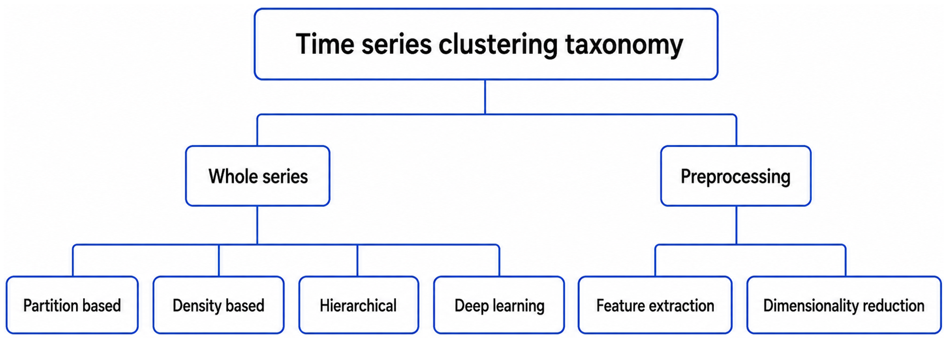
This paper aims to provide a comparative analysis of time series clustering models and their comparison with classification models. To ensure representativeness, various models from both groups—Whole Series and Preprocessing (see Figure 1)—were implemented. The Whole Series group included partition-based algorithms (Time Series K-Means and Time Series K-Medoids) and deep learning algorithms (AEFCN and AEResNet Clusterer). From the Preprocessing group, feature extraction algorithms such as Catch22Clusterer and TSFreshClusterer were applied.

The clustering models used in this study were selected to represent different approaches to time series clustering. The experiments were based on the aeon package, which provides implementations of time series learning methods and allows the models to be tested in one consistent framework. This was important because all models were evaluated on the same generated datasets, under the same noise and class settings.

The selected methods cover three main groups. TimeSeriesKMeans and TimeSeriesKMedoids represent distance-based methods, which operate directly on whole time series. Catch22Clusterer and TSFreshClusterer represent feature-based methods, where time series are first transformed into descriptive features. AEFCNClusterer and AEResNetClusterer represent deep learning-based methods, where clustering is based on learned latent representations.

This study does not include all possible time series clustering algorithms. Some methods, such as K-Shape, are important in the literature, but they were outside the final experimental set. Density-based methods, such as HDBSCAN, were also not included, because they are usually designed for feature-space data and require an additional representation or distance matrix when applied to time series. The final set of models was also influenced by practical limits, including running time, memory usage, and available computational resources. Therefore, the results should be interpreted as a comparison of selected representative methods rather than as a complete benchmark of all time series clustering algorithms.

3.1. Partition Based Models

Time Series K-Means and Time Series K-Medoids are partition-based clustering algorithms [15]. Partition-based models constitute a family of clustering methods that directly divide a dataset into k disjoint clusters, assigning each object to exactly one group in such a way that the total within-cluster cost is minimized.

Time Series K-Means is a variation of the traditional K-Means clustering algorithm proposed by MacQueen [16]. The main idea remains the same—to divide the data into k clusters by minimizing the sum of distances between observations and centroids:

$$J={\displaystyle \sum _{i=1}^n}\underset{1\le j\le k}{min}d(x_i,c_j)$$

(1)

Here, n denotes the number of time series in the dataset, and k is the number of clusters to be formed. Each time series $x_i$ is assigned to the cluster whose centroid $c_j$ minimizes the distance measure $d(x_i,c_j)$.

The distance function quantifies the dissimilarity between a time series and a cluster centroid. In the classical approach, centroids represent the geometric means of each cluster; however, in time series data we deal with barycenters, which are computed using specialized methods based on time series distance measures, such as DBA (Dynamic Time Warping Barycenter Averaging) [17], MSM (Move–Split–Merge) barycenter [18], ShapeDBA [19], or Soft-DTW barycenter [20]. A barycenter can be interpreted as an averaged (or prototypical) time series representing the group. The distance measure defines how similarity between time series is computed. It can be selected based on commonly used time series distance metrics such as DTW (Dynamic Time Warping), Euclidean, or Manhattan distance.

Time Series K-Medoids is an algorithm derived from the Time Series K-Means approach; however, instead of centroids, medoids are used [21]. Medoids correspond to actual observations from the dataset that best represent their respective clusters. Thus, the objective is to minimize the sum of distances between observations and medoids:

$$J={\displaystyle \sum _{i=1}^n}\underset{1\le j\le k}{min}d(x_i,m_j)$$

(2)

Here, $m_j$ denotes each medoid. The goal of the algorithm is to find a set of medoids $m_1,\dots ,m_k$ that minimize the total dissimilarity within clusters. A centroid is an averaged (not necessarily existing) representative of a cluster, whereas a medoid is a real data point that is most similar to all others in the cluster. The Time Series K-Medoids algorithm is more robust to outliers; however, it has a higher computational cost [22].

3.2. Deep Learning Models

The deep learning algorithms used in the experiment are AEFCN Clusterer and AEResNet Clusterer.

The AEFCN Clusterer (Auto-Encoder based Fully Convolutional Network Clusterer) is an algorithm that operates based on a convolutional autoencoder [23]. Its main objective is to learn an unsupervised data representation by compressing time series into a latent space and subsequently grouping these representations into clusters [24]. This process serves two purposes:

• To learn latent representations (embeddings) of time series;
• To group these representations into clusters in an unsupervised manner.

Unlike traditional clustering methods, it does not require the computation of pairwise distances between time series. Instead, it learns a feature space in which similar patterns are geometrically close to each other. The AEFCN architecture consists of three main components: an encoder, a decoder, and a clustering layer [5,25].

The AEResNet Clusterer (Auto-Encoder with Residual Network backbone) is based on an AutoEncoder–Residual Network architecture. It constitutes an extension of the AEFCN Clusterer [23]; however, instead of a conventional convolutional encoder–decoder structure, a Residual Network (ResNet) is employed [26]. The use of ResNet enables more effective learning of complex residual patterns, particularly in long or multivariate time series, and helps to mitigate the vanishing gradient problem in deeper networks [27].

3.3. Feature Extraction Models

Feature extraction models are the ones that change time series into statistical feature vector, and then proceed with standard clustering method such as K-means or K-medioids.

The Catch22 Clusterer is a clustering method that represents each time series as a set of 22 universal statistical and dynamical features known as CATCH22 (Canonical Time-series Characteristics) [28]. The Catch22 clustering process does not depend on the length of the time series, as it operates on a fixed set of features describing each series, such as autocorrelation, entropy, trends, and outliers. This approach captures the essential diversity of time-series behaviors, including statistical, nonlinear, and spectral properties.

The TSFresh Clusterer (Time Series Feature Extraction based on Scalable Hypothesis Tests) is, on the other hand, not limited to a predefined number of features. It can generate hundreds or even thousands of features and then selects only the most significant ones based on scalable hypothesis tests [29]. Similar to Catch22, it operates by creating a feature vector for each time series and then performing clustering in this feature space.

3.4. Classification Models

This study uses exactly the same set of time series classification models as in our previous work. The evaluated methods include both simple naive classifiers used as baselines and a selection of more advanced algorithms representing different families of approaches, including convolution-based (Rocket Classifier), dictionary-based (WEASEL Classifier), feature-based (Catch22 and TSFresh Classifiers), and interval-based methods (TimeSeriesForest Classifier). The naive methods assign class labels randomly, either with equal probability for each class or according to the class distribution in the dataset. This choice allows us to compare a broad spectrum of modeling strategies without making the experimental setup unnecessarily complex.

All models were run with the same settings as in the earlier study in order to keep the results directly comparable. The classification models are used here only as a benchmark and are not the main object of the present analysis. This benchmark includes naive baselines and several time series classifiers representing different methodological groups: convolution-based, dictionary-based, feature-based, and interval-based approaches. The main information needed to understand their role in this study is summarized above, while a more detailed description of their theoretical background and implementation details is provided in the previous classification study [1].

3.5. Accuracy Measures

All clustering models were evaluated using several external clustering metrics. Adjusted Rand Index, Rand Index [30], Mutual Information [31], Fowlkes–Mallows Index [32], Homogeneity, Completeness, and V-measure [33] were used. These measures compare the obtained clusters with the reference labels, but each of them looks at the result in a slightly different way. Rand Index is based on pairs of observations and checks whether two points are grouped together or separated in both partitions. Adjusted Rand Index is a corrected version of this measure and takes into account agreement that may appear by chance. Mutual Information describes how much information about the true classes is contained in the clustering result. Fowlkes–Mallows Index is also based on pairs of observations and combines pairwise precision and recall. Homogeneity means that one cluster should mainly contain observations from one class, while completeness means that observations from the same class should be placed in the same cluster. V-measure combines these two properties.

Classification-style metrics were also calculated, but only after aligning cluster labels with the true labels. This was done to make an additional comparison with classification models. The following measures were used: Accuracy [34], Balanced Accuracy [35], F1 Score [36], Precision, Recall, Jaccard Index [37], Cohen’s Kappa [38], and Matthews Correlation Coefficient [39]. Accuracy shows the proportion of correctly assigned labels. Balanced accuracy is based on recall calculated separately for each class. Precision shows how many objects assigned to a given class are correct, while recall shows how many objects from this class were found. F1 Score combines precision and recall. Jaccard Index measures the overlap between the predicted and true labels. Cohen’s Kappa and Matthews Correlation Coefficient are more conservative measures, because they also consider agreement that may happen by chance.

Since clustering labels do not have a fixed meaning, they first had to be matched with the reference class labels. For this purpose, the Hungarian Algorithm was used [40]. This step makes it possible to calculate classification-style metrics for clustering results. However, these values should be treated only as an additional reference. The matching is performed after clustering and is chosen to maximize agreement with the true labels. For this reason, the main interpretation of clustering quality in this paper is based mainly on clustering measures, especially Adjusted Rand Index and V-measure.

4. Data Simulations

This paper extends our previous research and uses exactly the same synthetic datasets. The data consist of artificially generated time series representing several basic waveform types, including sinusoidal, cosinusoidal, triangular, sawtooth, inverted sawtooth, and PWM signals. To better reflect real-world conditions, additive Gaussian noise with varying intensity was applied to all series. The same data generation framework as in the previous classification study was used intentionally. This allowed the clustering results obtained in the present paper to be compared directly with the classification results from the earlier work.

In the present study, the main elements of the data-generation procedure are described directly in order to make the experimental setup self-contained. Each synthetic dataset was built from predefined waveform classes. The considered waveform types included sinusoidal, cosinusoidal, triangular, sawtooth, inverted sawtooth, and PWM signals. For each dataset, a fixed set of waveform classes was selected, and the generated time series were assigned to these classes in a balanced way. Additive Gaussian noise was then added to the signal in order to increase the difficulty of the clustering task in a controlled manner. The noise level and the number of classes were varied separately, which made it possible to analyze their influence independently.

In total, 82 balanced datasets were constructed, differing in both the number of classes (ranging from two to six) and the noise level. This design makes it possible to analyze not only the influence of noise intensity, but also the effect of increasing class complexity on clustering performance. Each dataset contains 200 time series, with 1000 observations per series.

All datasets had the same basic size and time-series length. Each dataset contained 200 time series, and each time series consisted of 1000 observations. The number of classes varied from two to six, depending on the dataset configuration. Since the datasets were balanced, each class contributed the same number of time series within a given dataset. The reference class labels were retained only for external evaluation and benchmark comparison. They were not used during clustering model fitting.

Each dataset was generated by assigning time series to predefined waveform classes. The basic signal shapes were then modified by additive Gaussian noise with a selected intensity level. In this way, the class structure was known in advance, while the difficulty of the clustering task could be increased in a controlled way. The number of classes was changed separately from the noise level, which made it possible to analyze these two factors independently. The use of the same generated datasets as in the previous classification study was important, because it allowed the clustering results obtained here to be compared directly with the classification benchmark.

The datasets and their parameters were kept identical to those used in the previous study in order to ensure full comparability of the results. The data-generation framework was originally introduced in [1], but the main elements required to understand and reproduce the present clustering experiment are summarized in this section. The previous paper is cited as the source of the original classification benchmark, while the current manuscript provides the dataset structure and experimental logic needed for the clustering analysis.

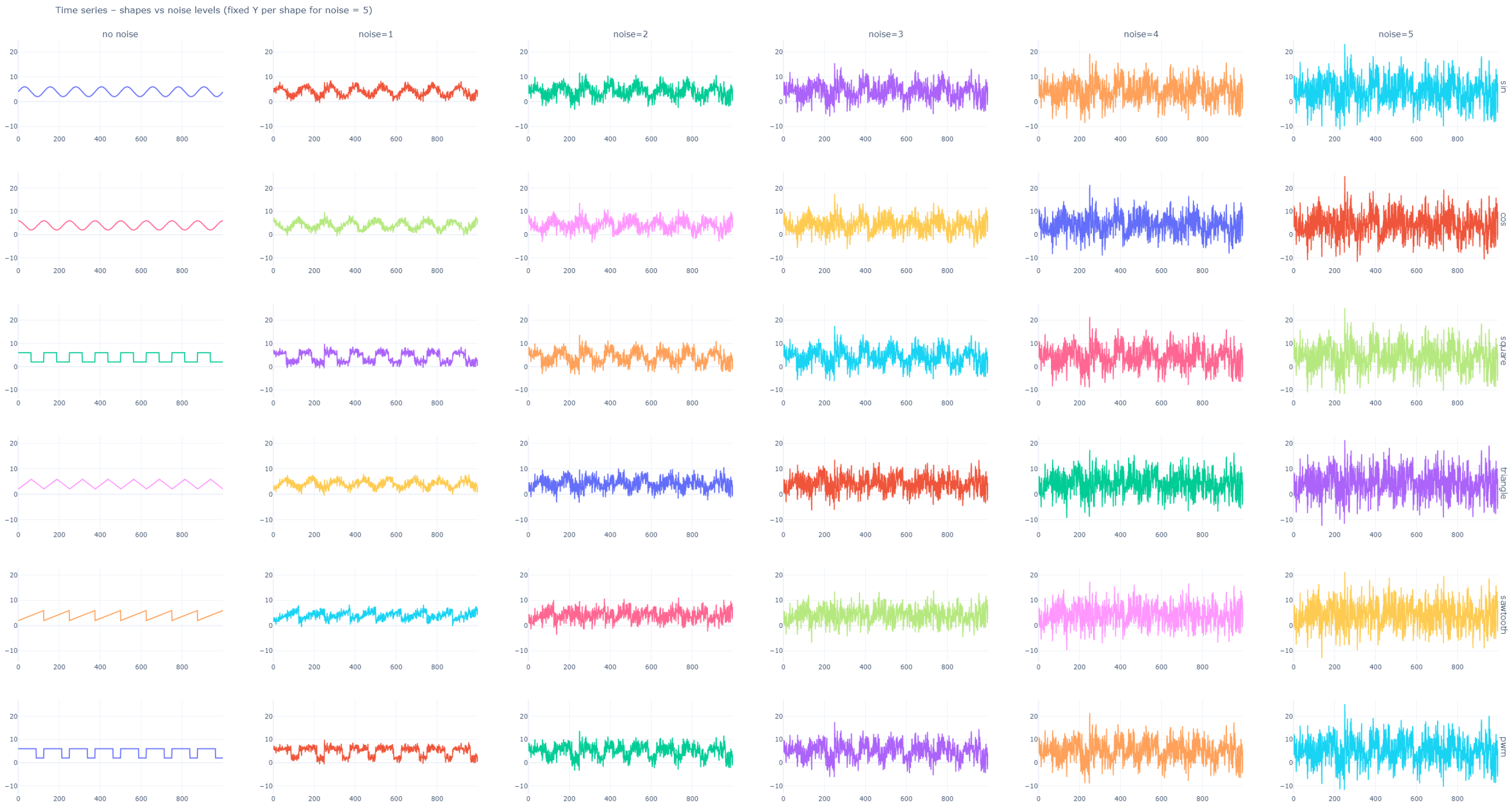
To make the generated data easier to interpret, examples of the used time series are presented in Appendix A. The examples show selected waveform types and illustrate how the signal changes when the noise level increases. These plots are not intended to represent all generated datasets, but they provide a visual example of the data structure used in the experiments.

Table 2. Example rows from the dataset-generation configuration used in the experiment.

Dataset ID	Length	Observations	Classes	Shapes	Noise Max
1	1000	200	2	PWM, cosine	5
2	1000	200	2	PWM, cosine	10
3	1000	200	2	PWM, cosine	15
4	1000	200	2	PWM, cosine	20
5	1000	200	2	PWM, cosine	25

shows an illustrative excerpt from the dataset-generation configuration. The full experiment contained 82 balanced datasets, while the table presents only selected initial rows to show how the datasets were defined. In particular, the table includes the length of the time series, number of observations, number of classes, waveform types, noise distribution, noise level, and cross-validation setup.

The table is included only as an example of the configuration format. The remaining datasets were created in the same way, with different numbers of classes, waveform combinations, and noise levels. The general dataset-generation code and data are available in the project repository, while additional implementation details can be provided upon reasonable request.

5. Experimental Results

This section presents the experimental results of the clustering study and compares them with the classification results obtained in our previous work. First, the performance of the considered clustering methods (including Time Series K-Means, Time Series K-Medoids, AEFCN, AEResNet, Catch22Clusterer, and TSFreshClusterer) is analyzed in detail. Next, a comparative analysis is presented across three groups of models: naive baselines, classification models, and clustering methods.

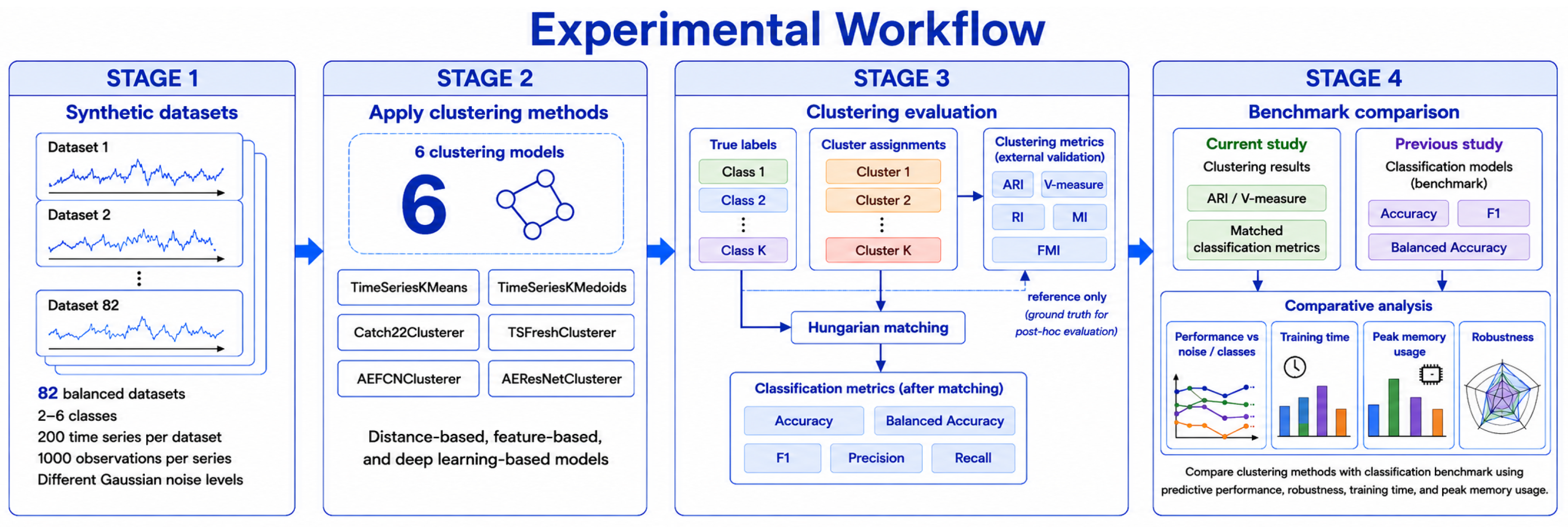
Figure 2 summarizes the main stages of the experimental procedure. The study begins with the generation of synthetic time-series datasets with controlled numbers of classes and different levels of Gaussian noise. These datasets are then used to test six clustering methods, selected to represent distance-based, feature-based, and deep learning-based approaches. After clustering, the obtained cluster assignments are evaluated in two ways. First, external clustering validation measures are computed, with the reference labels used only as post hoc ground truth. Second, cluster labels are aligned with the reference labels using the Hungarian algorithm, which allows auxiliary classification-style metrics to be calculated. In the final stage, the clustering results are compared with the classification-model benchmark from the previous study. This comparison includes not only predictive performance and robustness to noise and class complexity, but also computational aspects such as training time and peak memory usage. To make the current manuscript more self-contained, the full experimental workflow is summarized below, even though the data generation framework and classification benchmark are connected with the previous study [1].

The overall experimental procedure is summarized in Algorithm 1. It should be noted that reference labels were not used during clustering model fitting. They were used only after clustering to evaluate the obtained partitions and to compute auxiliary classification-style metrics after Hungarian label matching.

The training and evaluation process was organized in the same way for all clustering models. For each generated dataset, the selected clustering methods were fitted using the hyperparameter configurations defined in Table 3. The models were trained without using class labels. After fitting, the obtained cluster assignments were evaluated with external clustering metrics. Then, cluster labels were aligned with the reference labels using the Hungarian algorithm, which made it possible to calculate auxiliary classification-style metrics. External clustering metrics included ARI, V-measure, RI, MI, and FMI, while auxiliary classification-style metrics included Accuracy, F1, Precision, and Recall.

After the model had been fitted, the validation time series were assigned to clusters using the fitted model. The validation fold was not used to fit the model again, and the reference labels were not used during this assignment step. The exact assignment procedure depended on the type of clustering method. In distance-based methods, validation series were assigned to the closest learned centroid or medoid using the selected distance measure. In feature-based methods, validation series were first transformed into the same feature space and were then assigned by the fitted clustering estimator. In deep learning-based methods, validation series were first mapped to the learned representation and were then assigned by the clustering component of the model. Thus, the internal assignment step differed between model families, but the evaluation procedure was the same for all methods: the model was fitted on the training folds, clusters were assigned to the validation fold, and reference labels were used only after that for evaluation.

Algorithm 1 Experimental procedure
Require: Synthetic datasets $\mathcal{D}$, clustering methods $\mathcal{M}$, parameter grids ${\mathcal{P}}_m$, reference labels y
Ensure: Aggregated performance, computational cost, and benchmark comparison
1:	Generate synthetic datasets for all class numbers and noise levels
2:	for all  $D\in \mathcal{D}$ do
3:	Split D into 10 folds
4:	for all $m\in \mathcal{M}$ do
5:	for all $p\in {\mathcal{P}}_m$ do
6:	for $r=1$ to 10 do
7:	Use fold r for validation and the remaining folds for training
8:	Fit clustering model m with configuration p on the training time series only
9:	Record training time and peak memory usage
10:	Assign validation time series to clusters using the fitted model and obtain ${\widehat{c}}_r$
11:	Compute external clustering metrics
12:	Apply Hungarian label matching using ${\widehat{c}}_r$ and validation labels
13:	Compute auxiliary classification-style metrics  ▹ Accuracy, F1, Precision, Recall
14:	end for
15:	Aggregate validation metrics across the 10 folds for configuration p
16:	end for
17:	Select the best configuration for m using the highest mean validation ARI
18:	end for
19:	end for
20:	Aggregate results across datasets, noise levels, class numbers, methods, and folds
21:	Compare clustering results with the classification benchmark
22:	Analyze performance, robustness, training time, and peak memory usage

The dataset used in this study should be understood as a controlled experimental dataset. It was not designed to cover all possible real-world time series patterns. Instead, it was created to test the behavior of clustering methods under specific and repeatable conditions. The main aim was to analyze how the methods react when the noise level and the number of classes change separately. For this reason, the generated datasets were suitable for the purpose of this study, because they provided controlled variation in the two factors that were central to the experiment.

At the same time, the size of the dataset was selected with computational feasibility in mind. The full experiment included 82 balanced datasets, several clustering methods, multiple hyperparameter configurations, and a fold-based evaluation procedure. Each dataset contained 200 time series with 1000 observations per time series. This setting provided enough variation to compare the methods under different noise and class-complexity conditions, while still allowing the full experiment to be executed with the available computational resources. The results should therefore be interpreted as a controlled simulation study, not as a claim that the same dataset size is sufficient for every practical clustering problem.

5.1. Computational Resources

The experiments were carried out on the Topola high-performance computing cluster at the University of Warsaw. The cluster is based on Intel Xeon CPUs and NVIDIA Tesla V100 GPUs. The same computational platform was used in the previous classification study [1], which helped to keep the comparison between clustering and classification consistent. In the present paper, the computational analysis focuses on two practical aspects: training time and peak memory usage. Training time was recorded for each model configuration and then summarized across folds and datasets. Peak memory usage was measured to compare the resource requirements of different model families. This was especially important because the analyzed methods differ strongly in computational complexity, from lightweight feature-based methods to deep learning-based clustering models.

The experiments were implemented in Python 3.11.9. The clustering models were run using the aeon [41] package version 1.2.0. Data processing, statistical analysis, and visualization were performed using NumPy 1.24.3, pandas 2.0.3, and matplotlib 3.10.0. The source code and generated datasets are available in the GitHub repository reported in the Data Availability Statement.

5.2. Clustering Models’ Results

To obtain more stable estimates of clustering performance, a 10-fold fold-based evaluation protocol was used. This procedure should be understood as an external validation protocol for a controlled synthetic benchmark, not as classical supervised cross-validation and not as a fully unsupervised model-selection procedure.

For each generated dataset, the time series were divided into ten folds. In each iteration, nine folds were used as the training part and the remaining fold was used as the validation part. The clustering model was fitted only on the training time series. Class labels were not used during model fitting. After the model had been fitted, cluster assignments were obtained for the validation time series. The reference labels of the validation fold were then used only after clustering, in order to compute external clustering metrics and auxiliary classification-style metrics after Hungarian label matching.

The same fold partition was used for all clustering methods and all hyperparameter configurations within a given dataset. For each method, all configurations from the predefined grid reported in Table 3 were evaluated. The best configuration was selected according to the mean validation Adjusted Rand Index obtained across the ten folds.

It is important to emphasize that this ARI-based selection is not a fully unsupervised model-selection procedure. In real-world clustering applications, reference labels are usually unavailable, and hyperparameters would have to be selected using internal criteria, stability analysis, domain knowledge, or other unsupervised procedures. In the present study, the use of ARI for configuration selection is possible only because the datasets are synthetic and labelled. Therefore, the procedure should be interpreted as an external benchmark selection protocol used for controlled comparison, rather than as a general recommendation for practical unsupervised clustering.

The parameter n_clusters was not tuned freely. It was fixed to the known number of classes in each generated dataset. This decision was made because the purpose of the experiment was to evaluate whether the clustering methods could recover the predefined class structure under different noise levels and class-complexity settings. All remaining hyperparameters were selected from the grid shown in Table 3.

For statistical comparison of the methods, non-parametric testing was used, because the metric values were not assumed to be normally distributed. After the global comparison, Dunn’s post hoc test was applied to identify groups of methods with statistically significant differences. The significance level was set to (p < 0.05).

All models were implemented using the aeon package [41] in Python. For each method, several hyperparameter configurations were evaluated, as summarized in Table 3. The hyperparameter grid was prepared in the initial stage using an expert-based approach. The selection was based on the architecture of the models implemented in the aeon package, the values supported by these implementations, and the practical feasibility of running the full experiment. Since the study included many generated datasets, several noise levels, different numbers of classes, and cross-validation folds, the grid was not designed as an exhaustive search over all possible values. Instead, it was selected as a compromise between model coverage, computational cost, and the expected gain in clustering quality.

For TimeSeriesKMeans and TimeSeriesKMedoids, several distance measures were tested. The selected distances were chosen from the measures available in the aeon implementations and from commonly used distances for time series data. Elastic distances, such as DTW, MSM, ERP, EDR, and LCSS, were included because they can compare time series even when similar patterns are slightly shifted or locally distorted. Euclidean distance was included as a simpler baseline distance. In the case of TimeSeriesKMedoids, shift-scale distance was also tested, because it can account for differences in shift and scale between time series. This set of distances made it possible to compare different types of time series similarity without making the experiment too large computationally.

Table 3. Hyperparameter configurations explored for each clustering model.

Model	Hyperparameters
Time Series K-Means	n_init = 10; max_iter = {100, 200}; window = 0.2; n_clusters;
	distance = {“msm”, “dtw”, “edr”, “lcss”, “erp”}.
Time Series K-Medoids	n_init = 10; method = {“alternate”, “pam”};
	max_iter = {300, 500}; n_clusters.
	distance = {“msm”, “dtw”, “edr”, “lcss”, “erp”, “euclidean”, “shift_scale”}.
AEFCN	kernel_size = {[3,3]}; latent_space_dim = {32, 64, 128};
	n_epochs = {500, 2000, 5000}; n_filters = {[64,64]};
	n_layers = 2; n_clusters.
AEResNet	kernel_size = [3,3,3]; n_conv_per_residual_block = 3;
	n_epochs = {500, 2000}; n_filters = {[64,64], [64,64,64,64,64]};
	n_residual_blocks = {2, 5}; n_clusters.
Catch22 Clusterer	catch24 = {True, False}; n_clusters
	features = {“all”,
	[DN_HistogramMode_5, CO_f1ecac, SB_BinaryStats_mean_longstretch1],
	[CO_trev_1_num, CO_HistogramAMI_even_2_5, SB_TransitionMatrix_3ac_sumdiagcov]}.
TSFresh Clusterer	default_fc_parameters = {“minimal”, “efficient”};
	estimator = {200, 500}; n_clusters.

Table 3. Hyperparameter configurations explored for each clustering model.

Model	Hyperparameters
Time Series K-Means	n_init = 10; max_iter = {100, 200}; window = 0.2; n_clusters;
	distance = {“msm”, “dtw”, “edr”, “lcss”, “erp”}.
Time Series K-Medoids	n_init = 10; method = {“alternate”, “pam”};
	max_iter = {300, 500}; n_clusters.
	distance = {“msm”, “dtw”, “edr”, “lcss”, “erp”, “euclidean”, “shift_scale”}.
AEFCN	kernel_size = {[3,3]}; latent_space_dim = {32, 64, 128};
	n_epochs = {500, 2000, 5000}; n_filters = {[64,64]};
	n_layers = 2; n_clusters.
AEResNet	kernel_size = [3,3,3]; n_conv_per_residual_block = 3;
	n_epochs = {500, 2000}; n_filters = {[64,64], [64,64,64,64,64]};
	n_residual_blocks = {2, 5}; n_clusters.
Catch22 Clusterer	catch24 = {True, False}; n_clusters
	features = {“all”,
	[DN_HistogramMode_5, CO_f1ecac, SB_BinaryStats_mean_longstretch1],
	[CO_trev_1_num, CO_HistogramAMI_even_2_5, SB_TransitionMatrix_3ac_sumdiagcov]}.
TSFresh Clusterer	default_fc_parameters = {“minimal”, “efficient”};
	estimator = {200, 500}; n_clusters.

The tested parameter grid should not be interpreted as an exhaustive search over all possible hyperparameter values. In several models, some parameters are connected with each other and changing one of them affects the reasonable range or practical meaning of another one. For example, in deep learning-based models, the number of epochs, latent space dimension, number of layers, and number of filters influence both model complexity and training time. In distance-based methods, the choice of distance measure strongly affects computational cost. For this reason, the final set of configurations was selected as a practical compromise between model coverage, computational feasibility, and the expected improvement in results.

The parameter n_clusters was defined separately for each dataset according to its known number of classes. This was done because the study compares clustering results with the reference structure of the generated data. The remaining parameters were tested using the grid presented in Table 3.

No additional denoising or smoothing preprocessing was applied before clustering. This decision was intentional, because the aim of the experiment was to observe how the selected clustering methods behave when the noise level increases. In this study, noise was treated as a controlled property of the data, not as an artifact removed before modeling. Some tested hyperparameters, such as the distance measure, feature set, latent space dimension, or number of training epochs, may influence the robustness of a model to noisy data. However, a full analysis of noise-mitigation strategies would require a separate experimental design, including preprocessing methods such as smoothing, filtering, or denoising representations.

Because the datasets are synthetic and have known reference labels, ARI-based configuration selection should be interpreted as an external benchmark selection protocol rather than as a fully unsupervised model-selection procedure. In real unsupervised applications, hyperparameters would need to be selected using internal criteria, domain knowledge, or stability analysis.

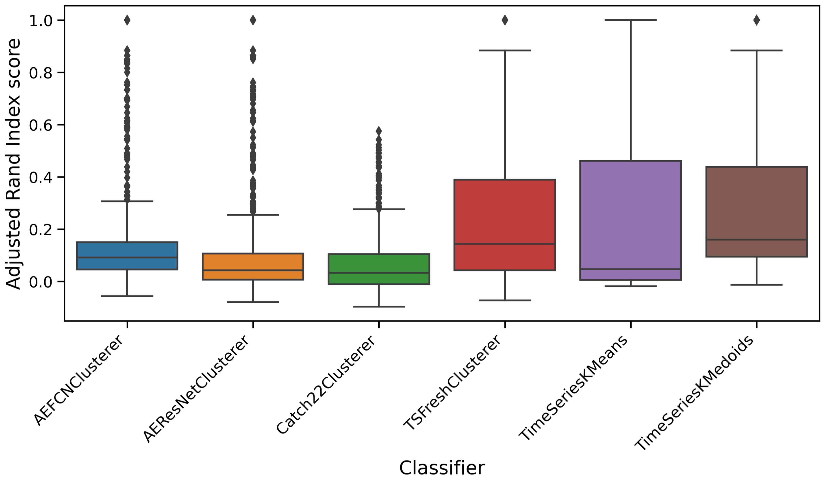
Figure 3 shows a boxplot of the Adjusted Rand Index values obtained across all clustering methods. The distribution of median ARI values indicates that distance-based approaches, and in particular Time Series K-Medoids, achieve the highest clustering quality in typical scenarios. Deep learning–based methods and the Catch22 Clusterer exhibit relatively low variance; however, their overall performance remains limited. The presence of a few high extreme values suggests that some methods are occasionally able to achieve nearly perfect scores, although this behavior is strongly dependent on the characteristics of the data.

Table 4. Results of Dunn’s post hoc test comparing clustering methods based on homogeneity. Different letters indicate statistically significant differences between groups ($p<0.05$).

Method	Measure	Group
Time Series KMedoids	0.3468	a
TSFresh Clusterer	0.3172	a
AEFCN Clusterer	0.2786	a
Catch22 Clusterer	0.2175	b
Time Series KMeans	0.1990	c
AEResNet Clusterer	0.1859	c

presents the results of Dunn’s post hoc test [42] for homogeneity. The analysis shows that TimeSeriesKMedoids, TSFreshClusterer, and AEFCNClusterer belong to the highest-ranked group (‘a’), meaning that no statistically significant differences were found between them. Catch22 Clusterer forms an intermediate group (‘b’). The lowest homogeneity values were obtained by TimeSeries KMeans and AEResNet Clusterer, which are both assigned to group (‘c’).

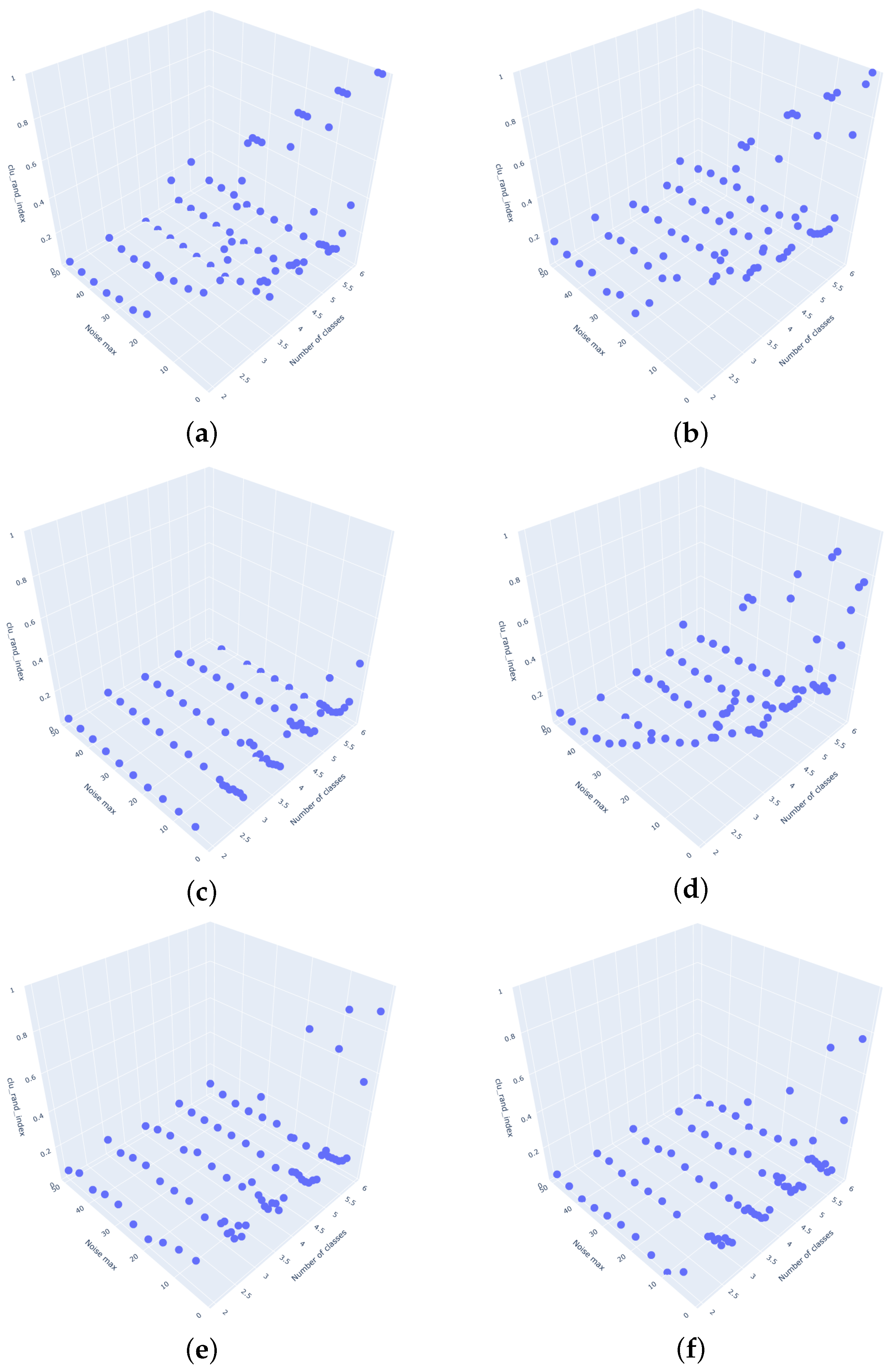
Figure 4 illustrates how the Adjusted Rand Index depends on both the number of classes and the noise level. The corresponding three-dimensional visualizations in the full format are available in the project repository at https://github.com/MariaSadowska/TSC_clustering_article.git (accessed on 20 April 2026). As the number of classes increases, a systematic decrease in clustering quality can be observed for all evaluated methods, reflecting the growing difficulty of the task with increasing class complexity. Across the entire range of class counts, Time Series K-Medoids consistently achieves the highest or near-highest ARI values.

An even stronger effect can be observed for the noise level. Even a moderate increase in noise leads to a noticeable degradation of clustering quality, particularly for feature-based methods and deep learning approaches. Distance-based methods, and especially Time Series K-Medoids, exhibit greater robustness to noise, maintaining relatively higher ARI values even at higher noise levels. This suggests that robustness to signal noise is a key factor influencing the effectiveness of time series clustering.

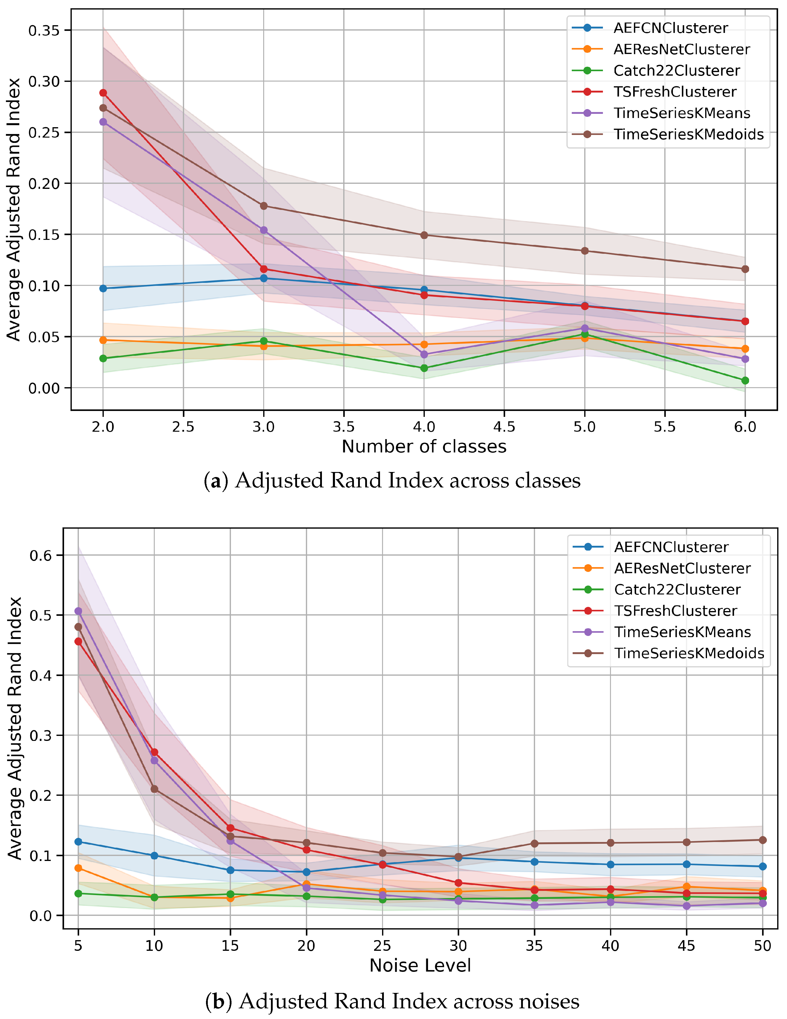
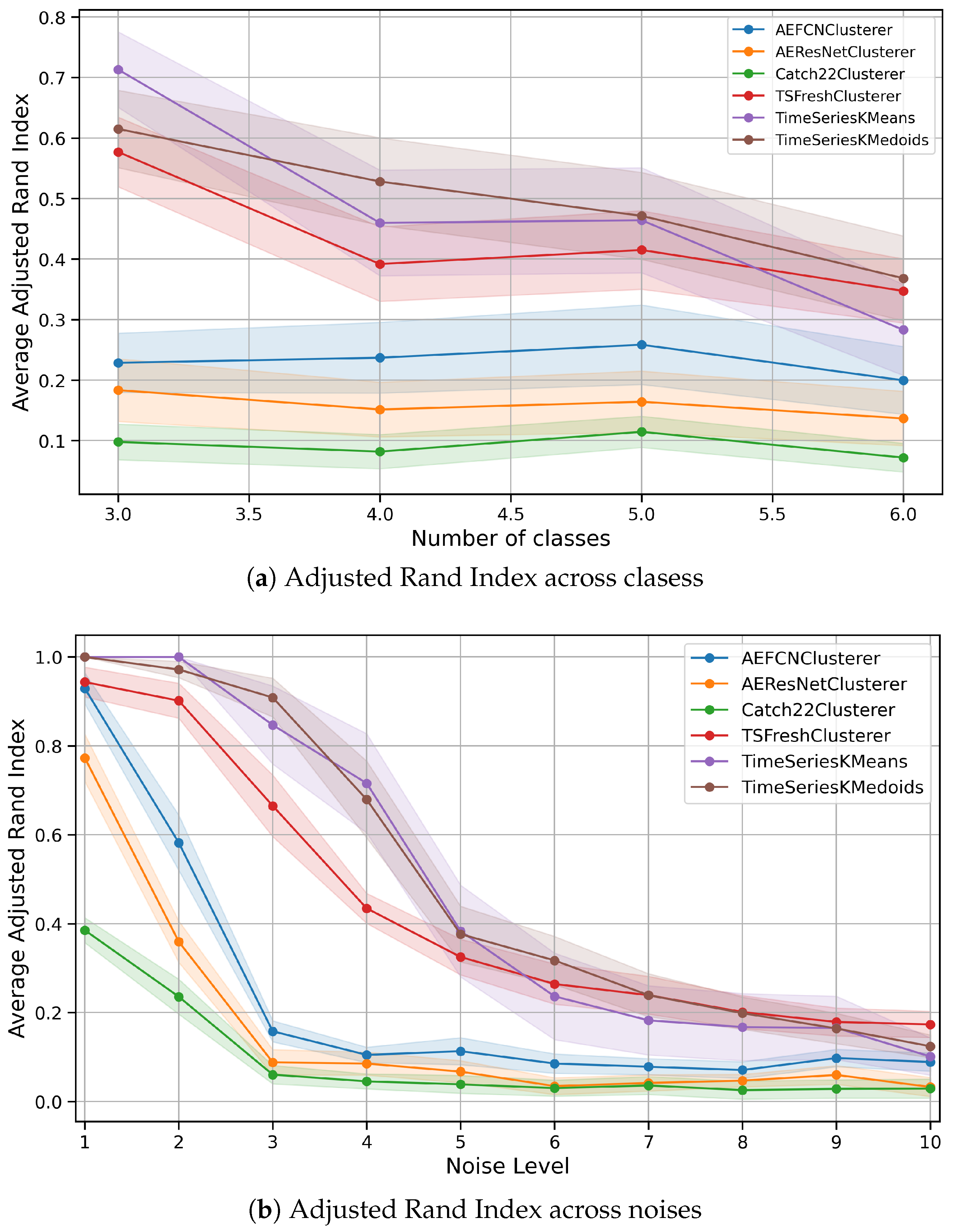
Figure 5 shows how the Adjusted Rand Index changes with the number of classes and with the noise level. In both panels, the lines represent mean ARI values, while the shaded areas show 95% confidence intervals. This makes it possible to assess not only the average trend, but also the variability of the results across the evaluated datasets and folds.

The results show that clustering quality generally decreases when the number of classes increases. This decrease is visible for most methods, although the size of the confidence intervals indicates that the stability of the methods is not the same. TimeSeriesKMedoids remains one of the most stable methods across the analyzed class numbers. TimeSeriesKMeans also performs well for some settings, but its performance becomes less stable when the task becomes more difficult.

The influence of noise is even clearer. When the noise level increases, ARI values decrease rapidly, especially between the lowest and moderate noise levels. The confidence intervals support this interpretation, because the downward trend is visible not only in the mean values, but also in the uncertainty ranges. Distance-based methods, especially TimeSeriesKMedoids, keep higher ARI values than the remaining methods for most noise levels, while feature-based and deep learning-based methods stay at lower values.

Figure 6 presents the same relationship for a narrower and more detailed range of noise levels from 1 to 10 and for datasets with three to six classes. This view is useful because the strongest performance drop occurs at the beginning of the noise scale. The confidence intervals show that the difference between the best distance-based methods and the remaining approaches is most visible for low and moderate noise levels.

For small noise values, TimeSeriesKMeans and TimeSeriesKMedoids obtain the highest ARI scores. However, when the noise increases, their performance also decreases. TimeSeriesKMedoids remains relatively more stable, while TimeSeriesKMeans shows a stronger drop. This supports the interpretation that the medoid-based representation is less sensitive to noisy observations than centroid-based averaging.

The deep learning-based and feature-based clustering methods do not show the same improvement in the low-noise setting. Their confidence intervals are also generally lower on the ARI scale, which suggests that in this experimental setup the learned or extracted representations were not able to preserve the waveform class structure as well as direct distance-based comparison.

Taken together, Figure 5 and Figure 6 indicate that noise level appears to be the dominant factor affecting clustering quality, outweighing the influence of the number of classes. While increasing class complexity leads to a gradual and predictable degradation in performance, noise induces much more abrupt and nonlinear declines that fundamentally challenge clustering effectiveness.

These observations further suggest that robustness to noise should be considered a key criterion when selecting clustering methods for time series data. In this respect, distance-based approaches—especially those relying on medoid representations—offer superior stability compared to centroid-based, feature-based, or deep learning methods.

5.3. Comparison of Clustering and Classification Results

In this section, the performance of clustering methods is compared with the results previously obtained for classification models and naive baselines. All experiments were run on the same datasets and in the same computational environment, so that the results are directly comparable. Since clustering is an unsupervised task, the Adjusted Rand Index (ARI) and V-measure are used as the primary clustering metrics, while accuracy after Hungarian label matching is treated only as a supplementary point of reference.

5.3.1. Accuracy After Label Alignment

After fitting the clustering models, Hungarian matching was applied to align cluster labels with the ground-truth classes. This makes it possible to report classification-style metrics, such as accuracy, for clustering results. However, these values should be interpreted with caution because the alignment procedure explicitly maximizes agreement with the true labels. This metric is useful because it allows clustering results to be compared with classification models on labelled datasets. However, it does not measure clustering quality in the same way as clustering-oriented metrics. The Hungarian algorithm finds the assignment between cluster labels and true labels that gives the best possible agreement. Because of this, the obtained accuracy is already optimized after the clustering step.

This can lead to an overly optimistic interpretation. A clustering method may obtain a relatively stable accuracy after label matching even when the real cluster structure is weak. This happens because the matching procedure can assign dominant clusters to the closest class labels, even if the partition itself does not represent the data structure well. In such a case, accuracy reflects the best post hoc label assignment more than the quality of the discovered clusters.

For this reason, structure-sensitive and chance-corrected measures are more appropriate for the main interpretation of clustering results. Adjusted Rand Index is useful because it compares two partitions at the level of pairs of observations and corrects for agreement that may occur by chance. This makes it more restrictive than simple label-aligned accuracy. V-measure is also important because it combines homogeneity and completeness. It checks not only whether clusters contain mainly one class, but also whether observations from the same class are assigned to the same cluster.

In this study, accuracy after Hungarian matching is therefore treated only as an auxiliary measure. It is reported to make comparison with classification models easier, but the main conclusions about clustering quality are based on Adjusted Rand Index and V-measure.

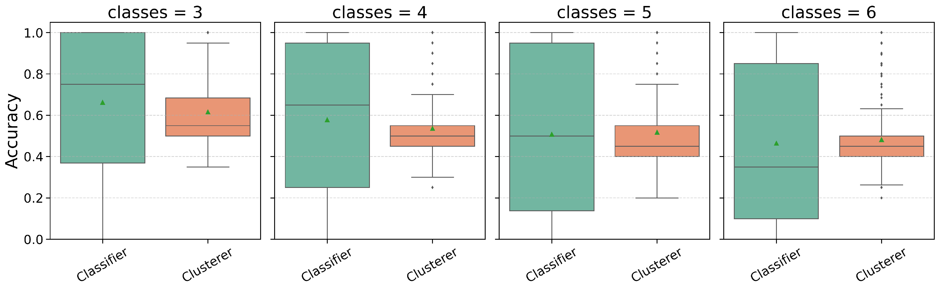
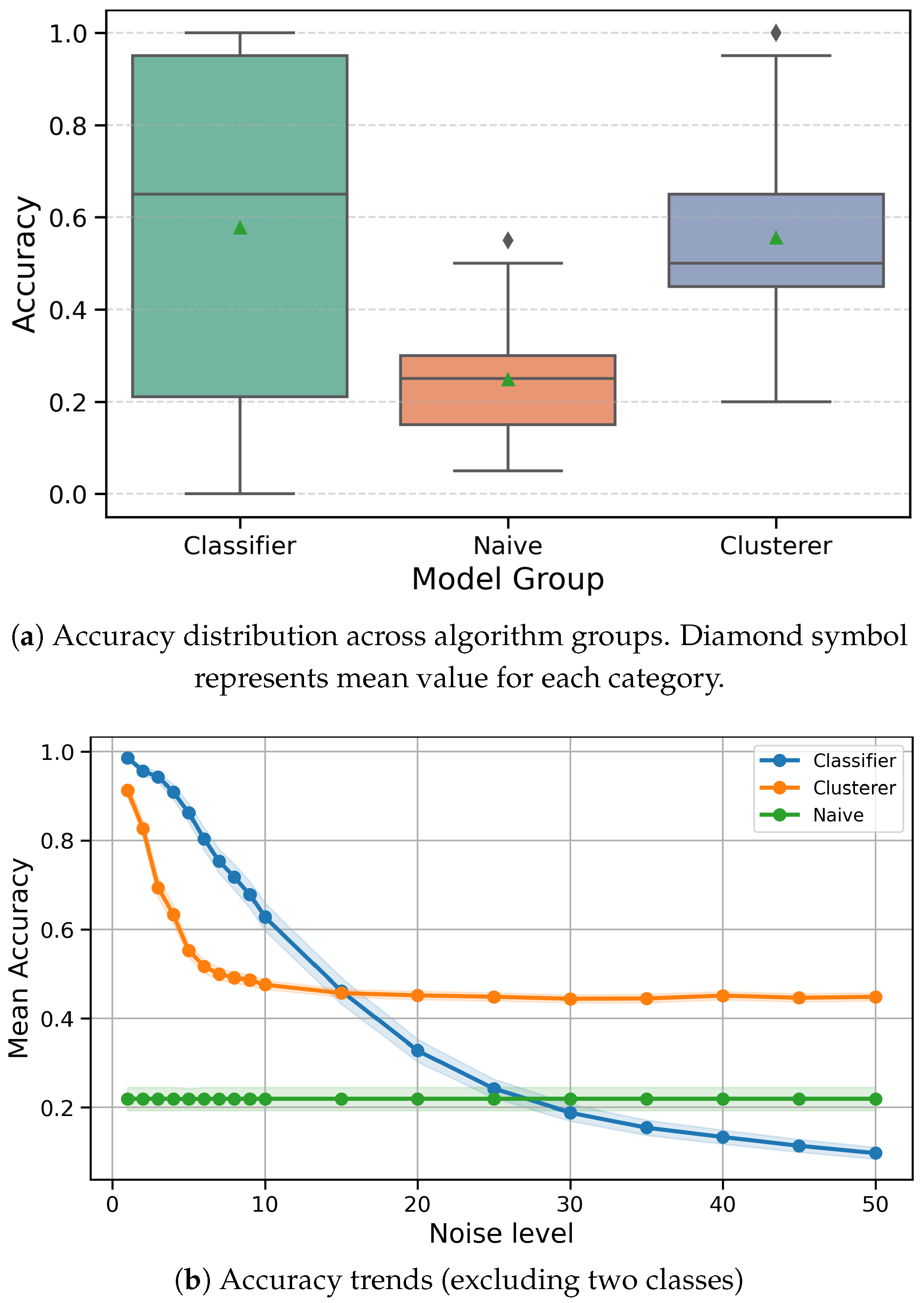
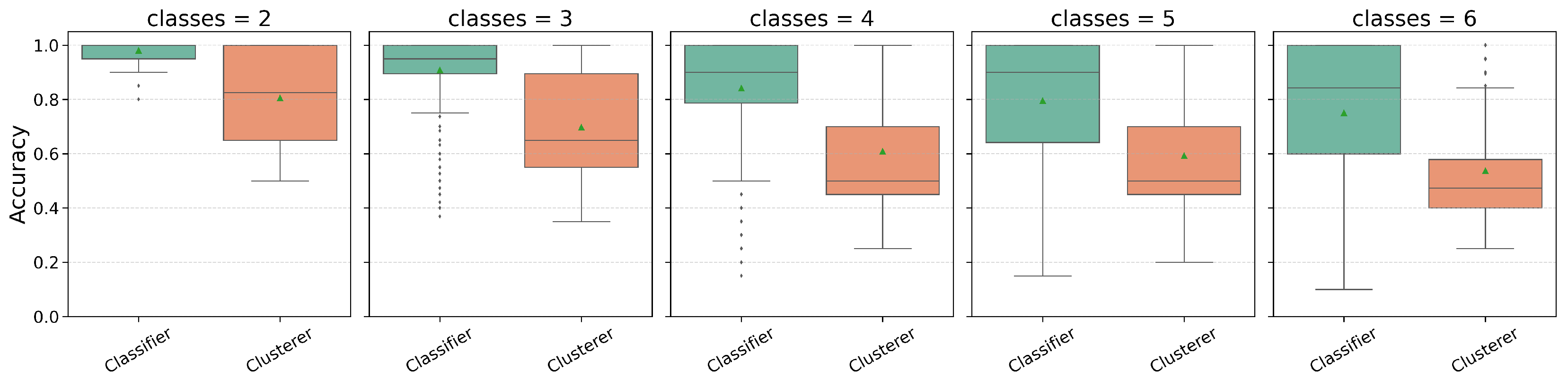
Figure 7a summarizes the distribution of accuracy values obtained after label alignment for both clustering and classification models. As expected, classification models achieve higher median and mean accuracy in this representation. However, the trend analysis shown in Figure 7b indicates that the relative behavior of the two groups changes with increasing noise. In particular, there exist noise regimes in which clustering models reach accuracy values comparable to, or occasionally higher than, those obtained by classification models. At the same time, in this representation, clustering methods consistently remain above naive random baselines. The 90% confidence intervals were added to this plot to make the variability around the mean accuracy trends more visible.

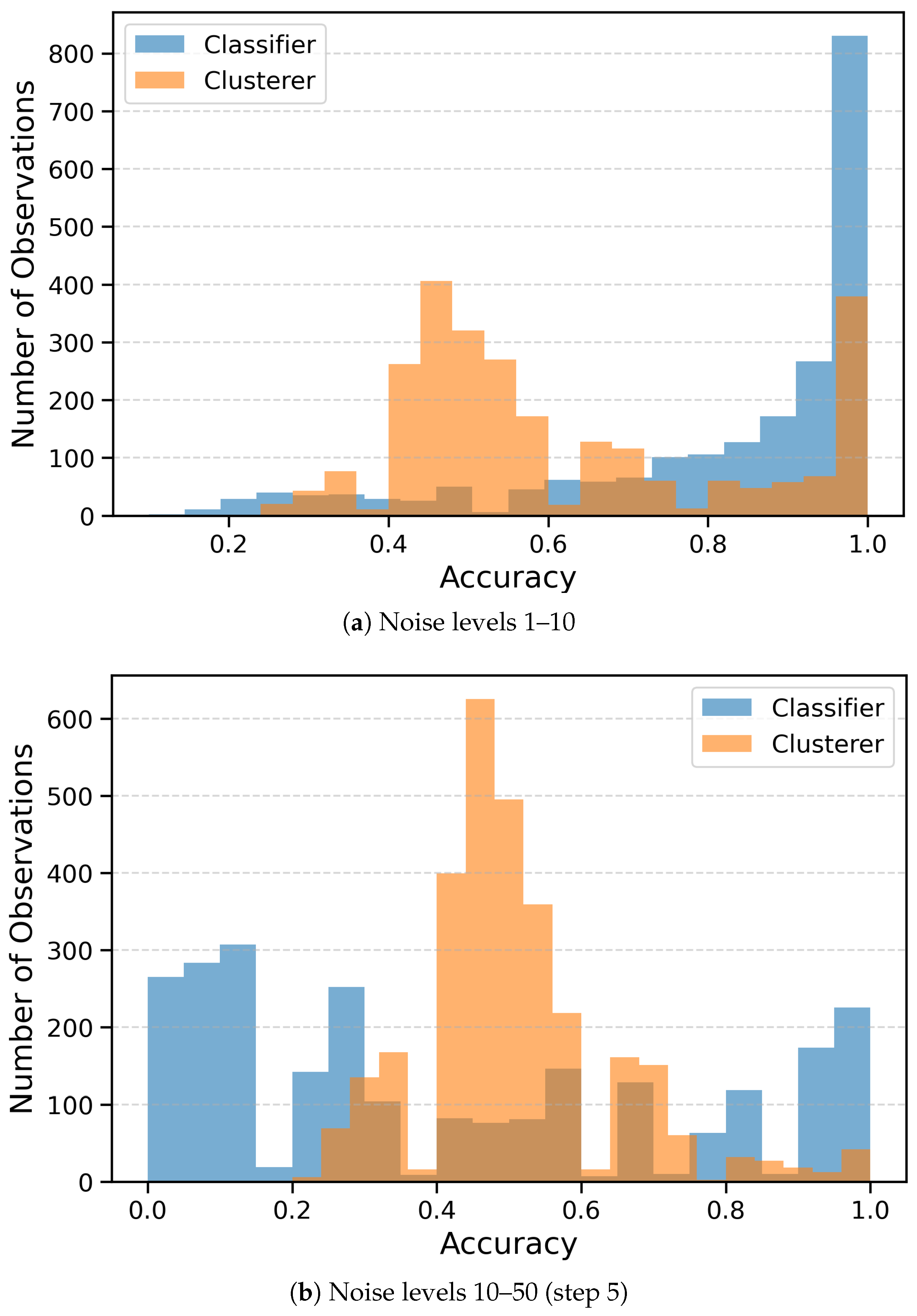
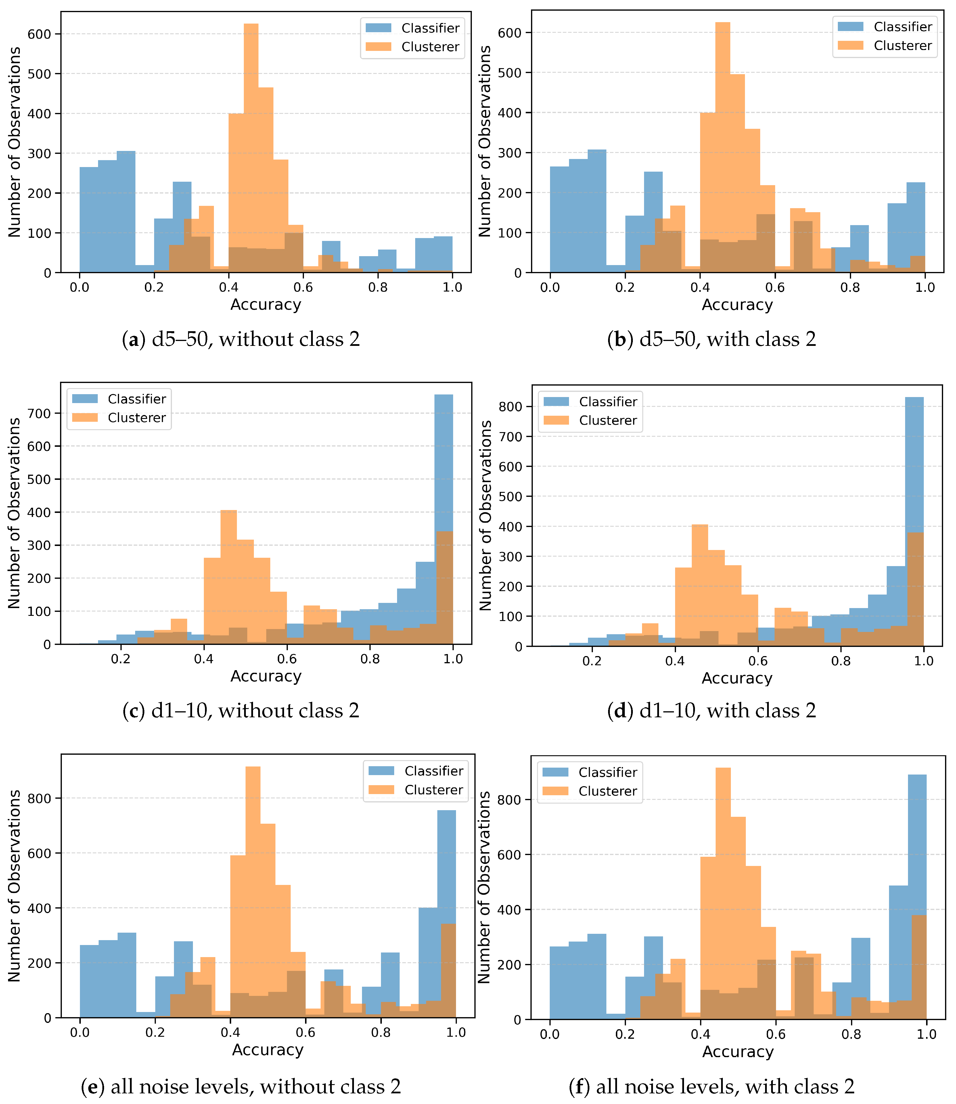
Figure 8 presents the distributions of accuracy values obtained after label alignment for two different noise ranges. For low noise levels, classification models achieve clearly higher values in this representation. With increasing noise, however, the separation between the two groups becomes less distinct and their accuracy distributions start to overlap. The two panels in Figure 8 are representative examples. The complete set of accuracy histograms for all noise ranges and class configurations is provided in Appendix A (Figure A8).

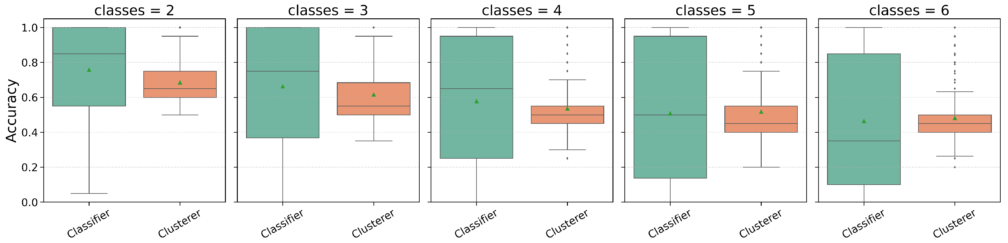
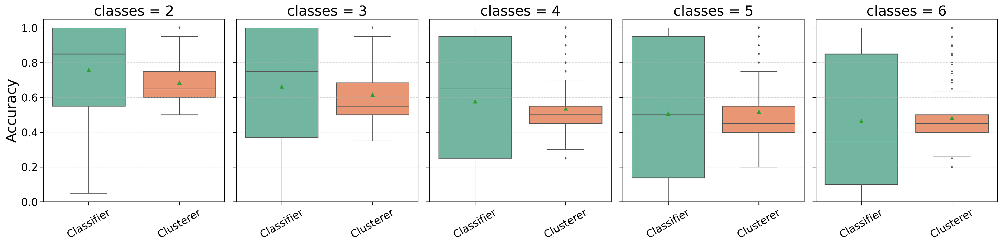
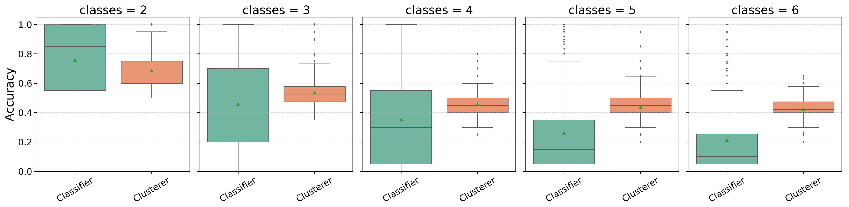
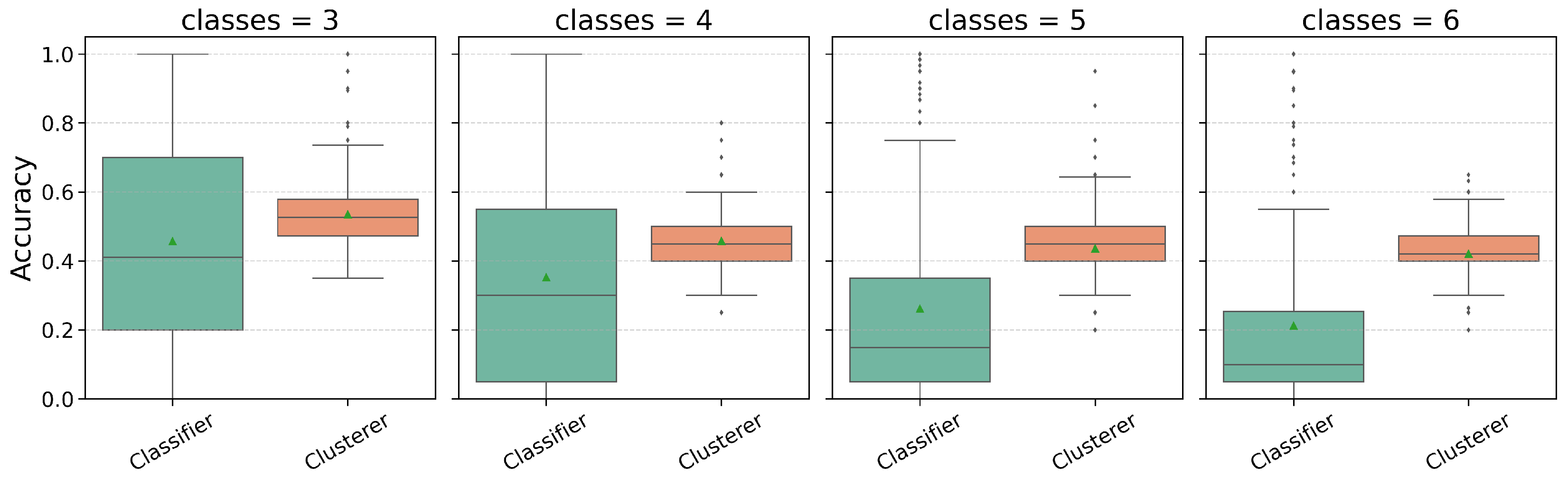
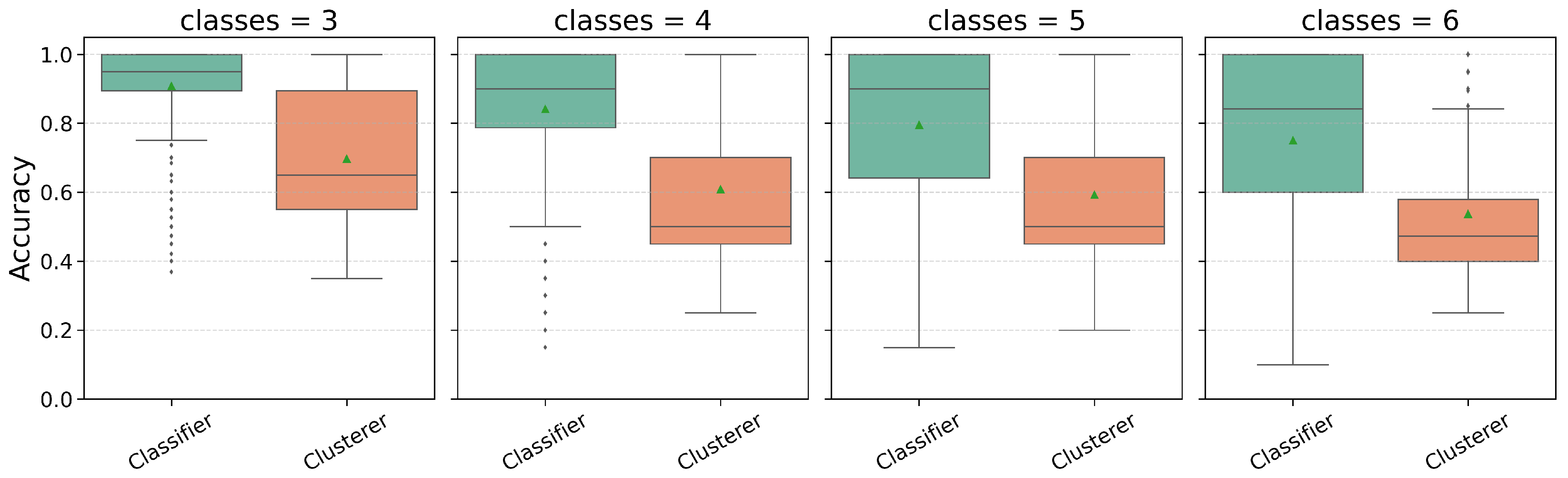
A similar tendency can be observed in Figure 9. The difference between classification and clustering models is most pronounced for a small number of classes and gradually diminishes as the number of classes increases. The full collection of boxplots for all experimental variants is shown in Appendix A (Figure A8).

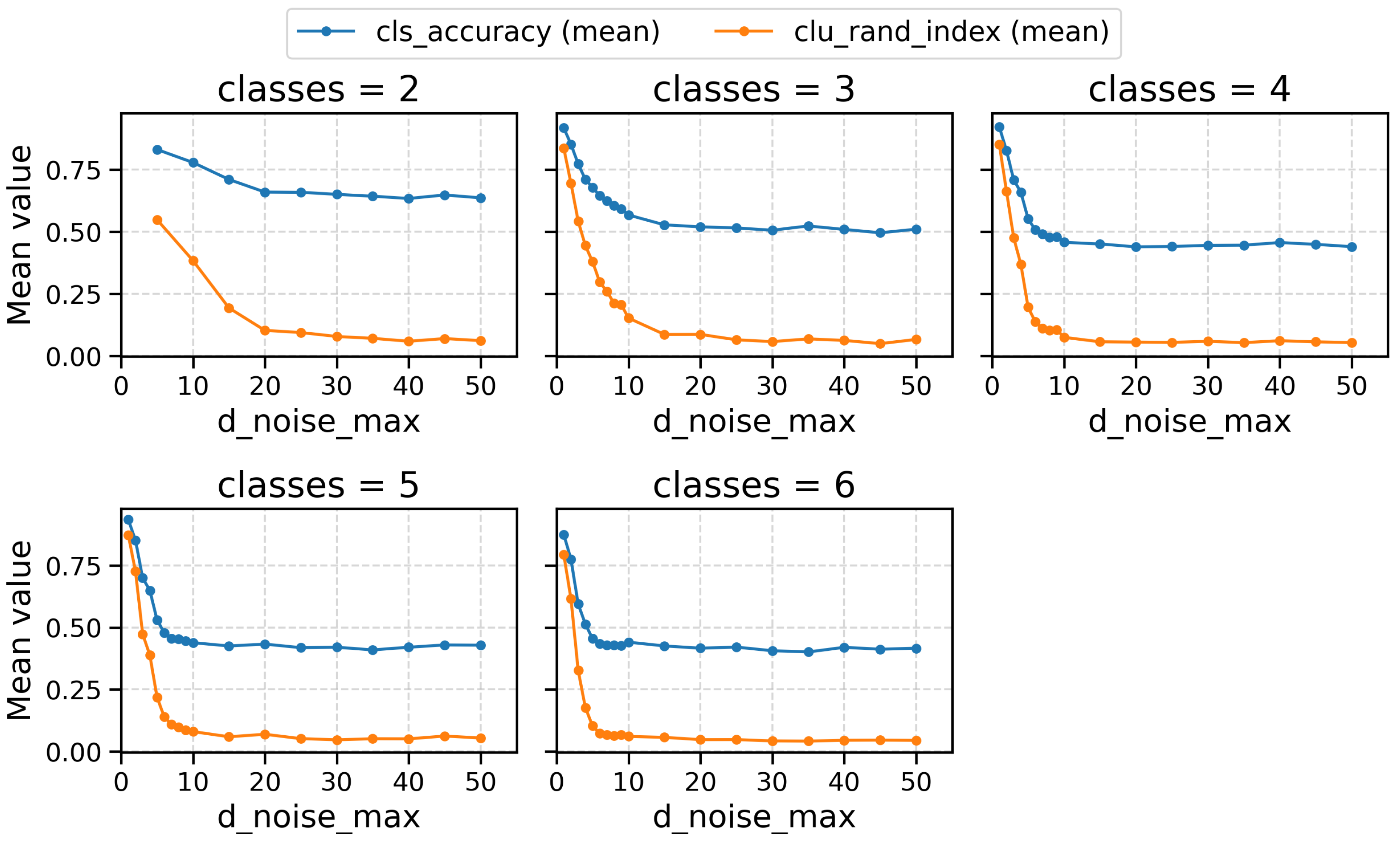
Figure 10 compares label-aligned accuracy with the Adjusted Rand Index. The results make it clear that ARI appears to provide a more restrictive and informative assessment of clustering quality. While accuracy remains relatively stable as the number of classes increases, ARI quickly exposes the degradation of the underlying cluster structure.

This observation shows that accuracy after Hungarian matching can give an overly optimistic picture of clustering performance. In particular, under high noise levels, nearly constant accuracy values may simply reflect the possibility of matching a few dominant clusters to class labels, rather than the presence of any meaningful clustering structure.

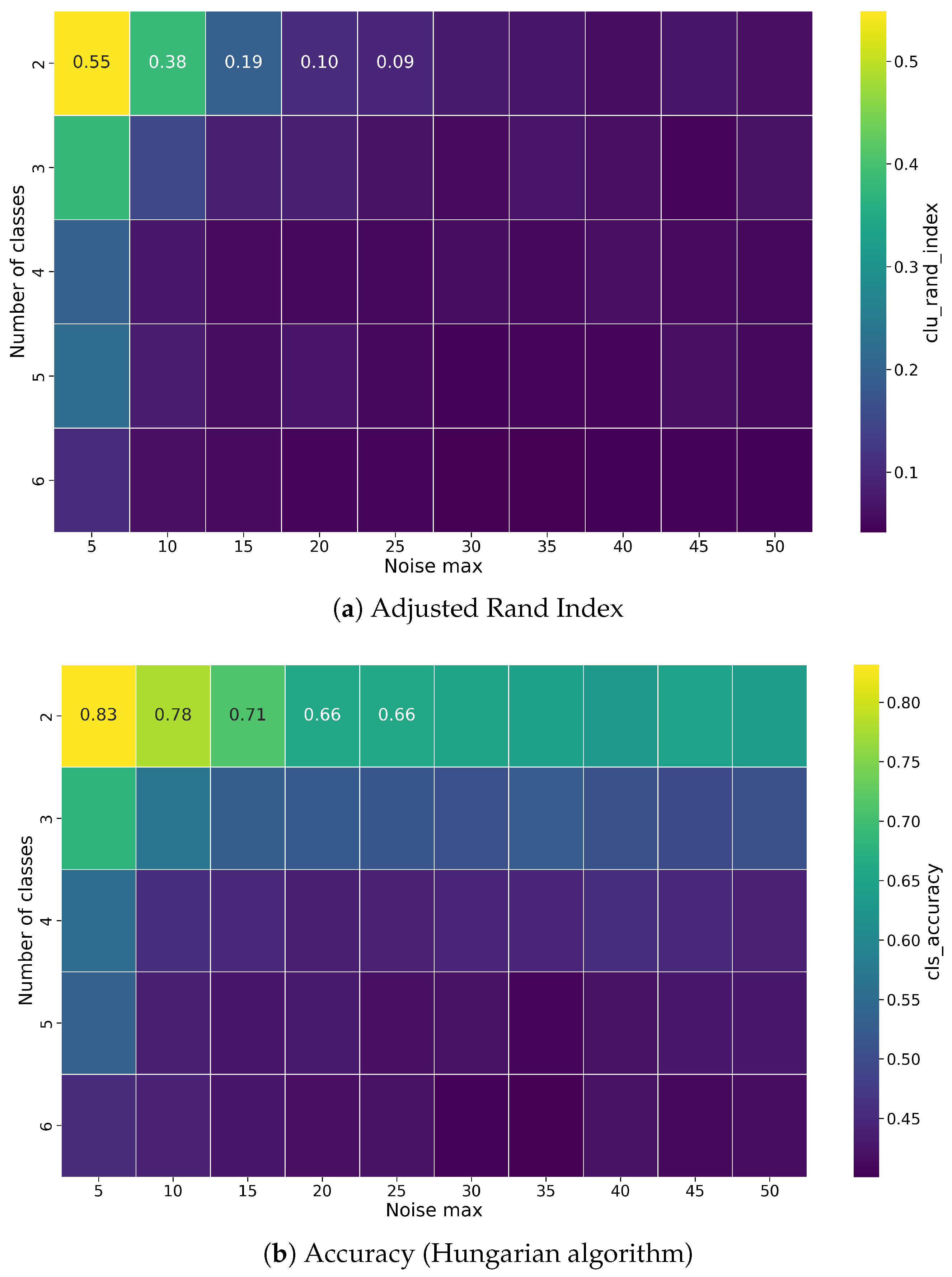
Figure 11 presents heatmaps of the Adjusted Rand Index and alignment-based accuracy for different numbers of classes and noise levels. With increasing noise, ARI values quickly drop toward zero, indicating clustering behavior close to random assignment. In contrast, accuracy after label alignment remains relatively stable, at a level of around 0.45.

This discrepancy shows that label-aligned accuracy does not capture the loss of the global cluster structure and may stay at a seemingly reasonable level even when the actual clustering quality has already deteriorated substantially.

Since cluster labels are arbitrary, Hungarian matching is used only to enable a label-aligned comparison with class labels. However, classification-style metrics computed after this alignment are inherently optimistic, as the matching procedure explicitly maximizes agreement with the ground truth. As illustrated above, this can lead to deceptively stable accuracy values even when chance-corrected measures such as ARI indicate near-random clustering.

For this reason, clustering performance in this study is assessed primarily using ARI and V-measure, while metrics computed after Hungarian matching are reported only as auxiliary indicators of external agreement under optimal label alignment.

The experimental study leads to several clear conclusions regarding time series clustering. Among the considered approaches, distance-based methods consistently achieve the strongest overall results, with Time Series K-Medoids standing out as the most reliable and robust method across a wide range of experimental settings. Feature-based and deep learning-based approaches, in contrast, show noticeably lower performance and greater sensitivity to data perturbations, particularly in the presence of noise. The results further indicate that clustering difficulty increases with both the number of classes and the noise level; however, noise clearly plays the dominant role. Even moderate noise levels result in a rapid deterioration of clustering quality for most methods, whereas the effect of increasing class complexity is more gradual and predictable. From a practical perspective, this highlights robustness to noise as a key factor determining the usefulness of a clustering method for time series data.

Applying Hungarian matching to align cluster labels with class labels makes it possible to compute classification-style metrics such as accuracy, but this procedure changes the nature of the evaluation. Rather than assessing the intrinsic quality of the recovered cluster structure, it primarily reflects how well a limited number of dominant clusters can be optimally assigned to known classes. In practice, the evaluation becomes closer to a post hoc label assignment problem than to a genuine assessment of clustering performance. The results show that accuracy computed after label alignment may remain at a seemingly reasonable level even when chance-corrected measures, such as the Adjusted Rand Index, indicate that the underlying cluster structure has already degraded to near-random. This illustrates that direct comparisons between clustering and classification based on Hungarian-matched accuracy can be misleading and require careful interpretation.

5.3.2. Computational Cost: Training Time and Memory Usage

In addition to predictive performance, computational cost was analyzed to assess the practical applicability of the considered methods. In this section, the models are compared in terms of training time and peak memory usage. Training times were calculated as the average training time across all folds for each model configuration, using the parameter setting that achieved the highest mean validation ARI for a given method. This was done in order to ensure a fair comparison between models under their best-performing setups. Peak memory usage was measured only once per model, since preliminary experiments showed that neither the number of classes nor the level of noise had a noticeable impact on memory consumption, and the observed differences between runs were negligible.

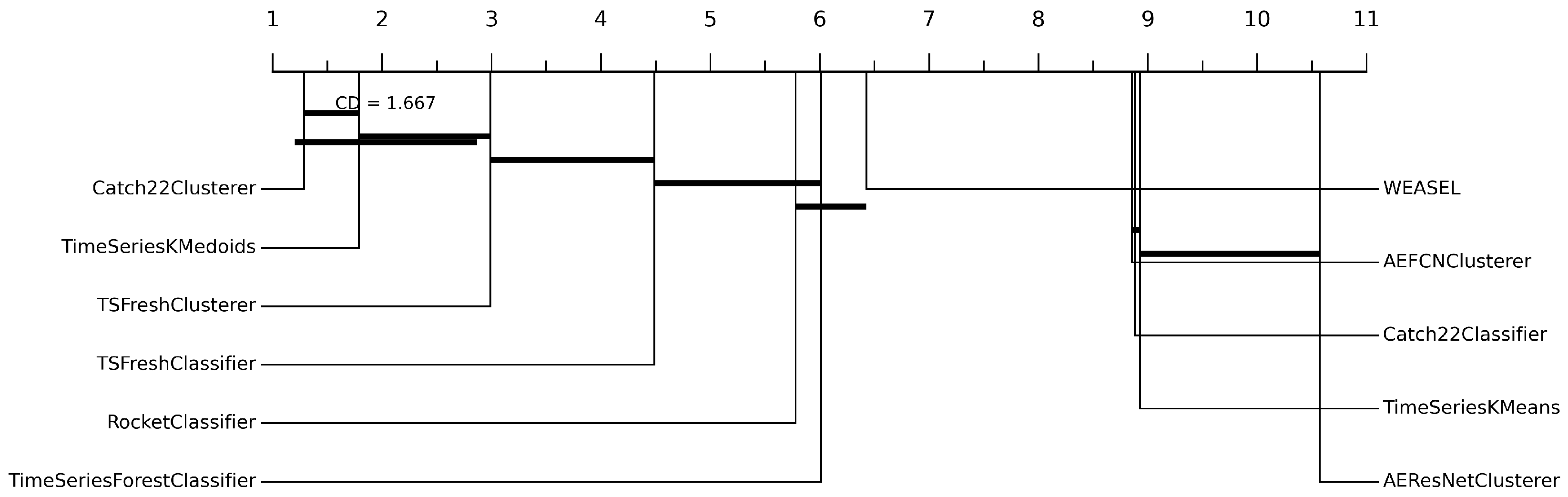
Figure 12 presents the Critical Difference (CD) diagram for training times. The methods were ranked on each dataset, where rank 1 corresponds to the shortest training time. The results indicate that Catch22Clusterer obtained the best average rank, followed by TimeSeriesKMedoids and TSFreshClusterer, which places them among the fastest methods considered in this study. In contrast, AEResNetClusterer, TimeSeriesKMeans, and AEFCNClusterer were ranked among the slowest approaches. The classification models TSFreshClassifier, RocketClassifier, and TimeSeriesForestClassifier formed an intermediate group with moderate computational cost. Importantly, the CD diagram also shows that not all pairwise differences are statistically significant; therefore, the results should be interpreted in terms of groups of methods with comparable training-time behavior rather than as a strict total ordering.

Table 5. Training times summary for clustering and classification models.

Model	Mean	Std	Median	Min	Max
Clustering models
Catch22Clusterer	0.027	0.004	0.027	0.018	0.033
TSFreshClusterer	0.060	0.005	0.058	0.055	0.082
TimeSeriesKMedoids	0.287	2.329	0.030	0.022	21.119
AEFCNClusterer	20.493	3.926	20.389	9.613	34.092
TimeSeriesKMeans	68.981	57.743	90.431	0.850	208.595
AEResNetClusterer	95.835	20.064	95.269	44.260	136.150
Classification models
TSFreshClassifier	3.031	0.963	2.777	0.075	7.128
RocketClassifier	4.201	1.886	4.444	0.620	7.682
TimeSeriesForestClassifier	5.073	0.865	4.912	4.037	10.813
WEASEL	5.861	2.640	6.531	0.633	9.487
Catch22Classifier	21.546	8.875	17.709	11.280	35.885

reports the descriptive statistics of training times for both clustering and classification models for each of the folds, including the mean, standard deviation, median, minimum, and maximum values. The results are consistent with the ranking-based comparison shown in the CD diagram. Among the clustering methods, Catch22Clusterer and TSFreshClusterer exhibited the shortest training times, with mean values of 0.027 and 0.060 min, respectively. TimeSeriesKMedoids also remained computationally efficient on average, although its large standard deviation indicates substantial variability across datasets. In contrast, AEFCNClusterer, TimeSeriesKMeans, and AEResNetClusterer were markedly more computationally demanding, with AEResNetClusterer showing the highest mean training time (95.835 min).

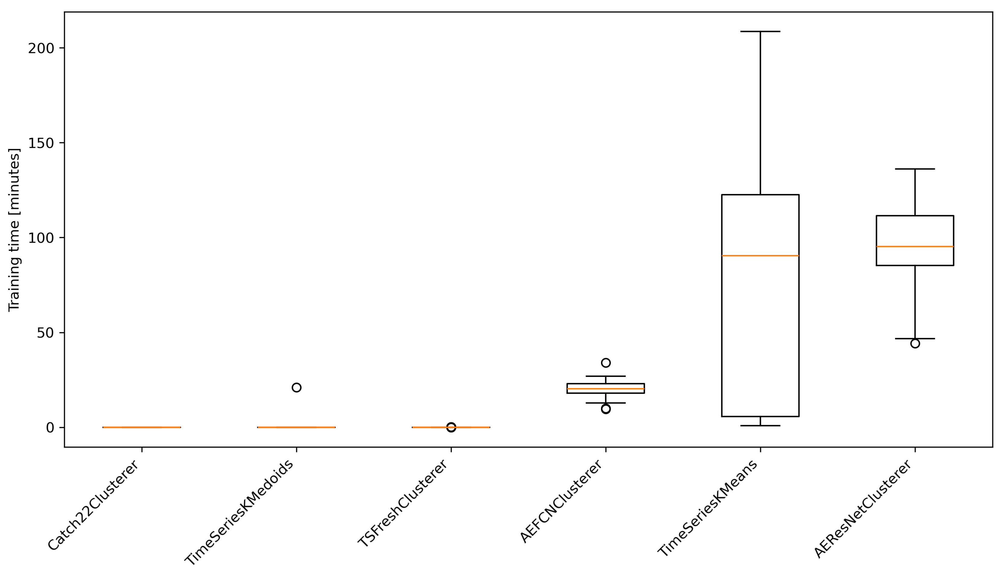
For the classification models, TSFreshClassifier achieved the lowest mean training time (3.031 min), followed by RocketClassifier, TimeSeriesForestClassifier, and WEASEL. Catch22Classifier was clearly the most time-consuming classifier, with a mean training time of 21.546 min. Overall, the descriptive statistics confirm that feature-based approaches were generally associated with lower computational cost, whereas deep learning and some distance-based methods required substantially longer training. A complementary boxplot of training times for the clustering models is provided in Appendix A (Figure A9). This visualization highlights the scale of the differences between methods particularly clearly, showing both the strong contrast in median training times and the substantial variability observed for the most computationally demanding approaches.

Table 6. Peak memory usage of the analyzed models (in MiB).

Group	Model	Peak Memory (MiB)
Clustering models	Catch22Clusterer	10.86
	TSFreshClusterer	46.90
	TimeSeriesKMedoids	47.34
	TimeSeriesKMeans	47.40
	AEFCNClusterer	487.41
	AEResNetClusterer	642.82
Classification models	Catch22Classifier	10.94
	TimeSeriesForestClassifier	17.10
	TSFreshClassifier	66.59
	CNNClassifier	72.02
	RocketClassifier	101.30
	WEASEL	367.38

summarizes the peak memory usage of the analyzed models. Among the clustering models, a clear separation can be observed between lightweight and memory-intensive approaches. Catch22Clusterer, TSFreshClusterer, TimeSeriesKMedoids, and TimeSeriesKMeans required relatively little memory, with peak usage below 50 MiB. In contrast, AEFCNClusterer and AEResNetClusterer were substantially more demanding, reaching 736.15 MiB and 784.81 MiB, respectively. This indicates that deep learning-based clustering methods impose a considerably higher memory cost than feature-based or classical clustering approaches. Notably, the number of clusters had no visible effect on peak memory usage in the clustering models. Across the tested configurations, memory consumption remained largely stable, suggesting that peak memory was determined mainly by the model architecture rather than by the number of clusters.

When compared with the classification models, the lighter clustering methods remain competitive in terms of memory usage and are comparable to the more efficient classifiers. However, AEFCNClusterer and AEResNetClusterer exceed the memory requirements of all classification models, including WEASEL, which was the most memory-intensive classifier. Overall, the results suggest that clustering models can be either highly memory-efficient or extremely memory-demanding, depending on the underlying methodological family, with deep clustering methods representing the most resource-intensive category.

6. Discussion

The results of this study should be interpreted in relation to previous work on time series clustering. Earlier reviews and benchmark studies show that the performance of clustering methods depends strongly on the selected representation, distance measure, and data characteristics. This is also visible in our experiment. However, the present study has a slightly different focus than many benchmark papers. Instead of testing methods mainly on existing real datasets, we used generated datasets where the noise level and the number of classes were changed separately. This makes it possible to observe more directly how selected clustering methods react to specific changes in data difficulty.

In this sense, the results complement previous benchmark studies rather than replace them. Large benchmark studies are useful because they show how clustering methods behave across many real datasets and application domains. Our study is more limited in terms of data diversity, but it gives more control over the source of difficulty. In real datasets, noise, class complexity, signal similarity, trends, seasonality, missing values, and outliers may appear at the same time. Because of this, it is often difficult to say which factor is mainly responsible for the decrease in clustering quality. The synthetic setting used here allowed us to isolate two factors: noise level and number of classes.

The experimental study leads to several important conclusions regarding time series clustering. Among the methods considered in this work, distance-based approaches achieved the most favorable overall results, with TimeSeriesKMedoids emerging as the most reliable and robust method across a broad range of experimental settings. In contrast, feature-based and deep learning–based approaches generally produced weaker results and showed greater sensitivity to data perturbations, especially in the presence of noise. This suggests that, for the type of data considered here, preserving pairwise similarity relationships is more effective than relying only on extracted features or learned latent representations.

A possible explanation for the strong performance of TimeSeriesKMedoids is related to the structure of the method itself. TimeSeriesKMedoids is a distance-based method, but unlike TimeSeriesKMeans, it does not represent clusters by averaged centroids or barycenters. Instead, each cluster is represented by a medoid, which is one real time series from the dataset. This difference is important for noisy data. When a centroid or barycenter is calculated from many noisy series, the representative shape can become blurred or distorted. A medoid is not averaged in this way, so it is less affected by local noisy fluctuations and remains an actually observed signal.

This also explains part of the difference between TimeSeriesKMeans and TimeSeriesKMedoids. Both methods use distances between time series, but the cluster representative is different. In TimeSeriesKMeans, the quality of the result depends not only on the distance measure, but also on how well the barycenter represents the cluster. Under higher noise, this barycenter may no longer describe the clean waveform shape well. In TimeSeriesKMedoids, the representative is selected from the existing time series, so the method is more conservative, but also more stable. In our experiment, where the class structure was based on waveform shapes, this stability was useful.

The performance of TimeSeriesKMedoids can also be connected with the type of data used in this study. The generated datasets were built from clearly defined waveform classes. Therefore, preserving the original shape similarity between whole time series was important. Distance-based methods work directly on the full time series and do not need an intermediate transformation. This is different from feature-based methods, where the signal is first reduced to a set of extracted characteristics, and from deep learning-based methods, where the signal is compressed into a learned latent representation. If this transformation loses part of the waveform information or becomes affected by noise, clustering quality may decrease.

Feature-based methods should be interpreted in this context. Catch22Clusterer and TSFreshClusterer first transform each time series into a vector of extracted features and then perform clustering in this feature space. This can be useful when the selected features describe the most important properties of the signal. It can also reduce computational cost compared with direct comparison of full time series. However, in the present experiment, the main class differences were strongly connected with the full waveform shape. If this shape information is only partly represented by the extracted features, or if noise affects the calculated characteristics, the clustering result may become weaker. This may explain why the feature-based methods did not outperform the best distance-based method.

The weaker performance of AEFCNClusterer and AEResNetClusterer should also be interpreted in this context. Both methods are based on autoencoder-type architectures. Their encoder compresses the input time series into a latent space, and clustering is then performed on this learned representation. Such architecture can be powerful, because it can learn complex features without manual feature design. However, in this study the models were trained in an unsupervised way, without class labels. This means that the encoder was not directly optimized to separate waveform classes. It mainly learned a representation useful for reconstructing or encoding the input signal.

When the noise level increases, this becomes a limitation. The autoencoder receives noisy time series as input, and part of the latent representation may describe noise-related variation instead of the underlying waveform class. In other words, the model may learn both the useful signal shape and the random perturbations. If this happens, the latent space becomes less clearly organized by class structure, and the clustering layer has a more difficult task.

The AEResNetClusterer has an even more complex architecture, because it uses residual blocks. Residual connections are useful in deep networks, because they help train deeper models and allow the network to learn more complex temporal patterns. However, this higher capacity is not always an advantage in small or noisy datasets. Each dataset in this study contained 200 time series, which is enough for a controlled experiment, but it may be limited for deep representation learning. With noisy inputs and limited data, a deeper model can become more sensitive to training settings and may not learn a stable class-separating representation.

AEFCNClusterer is simpler than AEResNetClusterer, because it is based on a fully convolutional autoencoder structure. Still, it has the same general limitation: the clustering depends on the quality of the latent representation. If the encoder does not separate the waveform types well, the later clustering step cannot fully recover this structure. This may explain why deep learning-based clustering methods required more computational resources but did not provide better clustering quality in the present experiment.

Therefore, the results do not mean that deep clustering methods are generally worse. They rather show that, for the controlled waveform datasets used here, direct shape-based comparison was more reliable than learned representation-based clustering. Deep learning methods may still be useful for larger datasets or for real-world time series with more complex patterns. In the present setting, however, robustness to noise and the use of real observed representatives gave TimeSeriesKMedoids an advantage.

The results also indicate that clustering difficulty increases with both the number of classes and the noise level, although the effect of noise is clearly stronger. While increasing the number of classes led to a gradual deterioration in performance, even moderate noise levels caused a rapid decline in clustering quality for most methods. This finding has an important practical implication: robustness to noise appears to be one of the key criteria in selecting clustering methods for time series data. In this respect, the advantage of distance-based methods, and particularly medoid-based approaches, was especially visible.

Another important observation concerns the relationship between predictive performance and computational cost. The methods that achieved the strongest clustering performance were not necessarily the most computationally expensive. In particular, TimeSeriesKMedoids combined strong clustering quality with relatively low peak memory usage, although its training time varied substantially across datasets. By contrast, the deep learning-based clustering models required much higher memory and training cost without providing a corresponding improvement in clustering quality. From a practical point of view, this means that more complex models do not automatically offer a better trade-off between effectiveness and computational efficiency.

The comparison between clustering and classification results should be understood as a benchmark reference, not as an assessment of two methods solving exactly the same problem. Although both groups of methods were evaluated on the same datasets, they solve fundamentally different tasks. Classification is supervised and uses known class labels during training. Clustering is unsupervised and tries to recover structure without access to class labels. Therefore, the comparison used in this paper shows how much of the class structure can be recovered without supervision under the same data conditions. It should not be interpreted as a direct competition between clustering and classification as if both approaches had the same objective.

This issue becomes particularly visible when Hungarian matching is used to align cluster labels with true class labels. Such alignment makes it possible to compute classification-style metrics, such as accuracy, for clustering outputs. However, this procedure changes the interpretation of the evaluation. Instead of measuring the intrinsic quality of the recovered cluster structure, it measures how well the obtained clusters can be optimally reassigned to the known labels after the fact. In this sense, the analysis becomes closer to post hoc label assignment than to a direct evaluation of clustering as an unsupervised learning task.

The results confirm that this distinction is not only theoretical but also practically important. Accuracy computed after label alignment may remain at a seemingly acceptable level even when chance-corrected clustering measures, such as the Adjusted Rand Index, indicate that the actual cluster structure has already deteriorated to near-random. This means that Hungarian-matched accuracy can give an overly optimistic picture of clustering quality, especially under high noise conditions. Therefore, it should be treated only as an auxiliary measure and not as the main basis for comparing clustering with classification.

From a methodological perspective, these findings suggest that clustering and classification should not be directly compared using the same primary evaluation metrics. Clustering is more appropriately assessed using structure-sensitive and chance-corrected measures, such as ARI or V-measure, whereas classification should be evaluated using standard supervised metrics. When a joint analysis of both paradigms is needed, a more informative approach is to compare their behavior under controlled changes in data difficulty, such as increasing noise or class complexity, rather than to compare them solely through label-aligned accuracy.

The results can be translated into several practical recommendations. If the time series have a clear shape-based structure and robustness to noise is important, distance-based methods should be considered first. In this study, TimeSeriesKMedoids was the most stable choice, especially because it uses real observed time series as cluster representatives. TimeSeriesKMeans may also be useful in less noisy settings, but it can be less stable when the barycenter is affected by noise.

Feature-based methods may be useful when the aim is to obtain a fast and compact representation of the time series, especially when direct distance-based comparison is too expensive. However, they should be used carefully when the main differences between classes depend on the full signal shape, because some information can be lost during feature extraction. Deep learning-based clustering methods should be considered mainly when larger datasets are available or when the expected structure is more complex than the waveform patterns analyzed here. In smaller and noisy datasets, their higher computational cost may not lead to better clustering quality.

The choice of evaluation measure is also important in practice. If the goal is to evaluate the recovered clustering structure, measures such as Adjusted Rand Index and V-measure should be preferred. Accuracy after Hungarian matching can be reported when clustering results are compared with a supervised classification benchmark, but it should remain an auxiliary measure. It should not be used alone to judge whether the clustering structure is meaningful.

Several limitations of this study should also be considered. First, all experiments were performed on synthetic datasets. This was useful for the aim of this paper, because the number of classes and the noise level could be controlled separately. At the same time, synthetic data do not fully reflect the complexity of real-world time series. In real applications, time series may contain trends, seasonality, regime changes, missing values, outliers, irregular sampling, and different types of noise. These effects were not fully represented in the present experimental setting.

The generated datasets were also based on a limited set of waveform types, including sinusoidal, cosinusoidal, triangular, sawtooth, inverted sawtooth, and PWM signals. These shapes make the class structure clear and allow controlled comparison, but they are simpler than many real signals. In addition, only additive Gaussian noise was used. Real data may contain non-Gaussian noise, local disturbances, outliers, or changes in variance over time. Because of this, the conclusions should be interpreted mainly as results from a controlled simulation study, not as direct evidence of performance on all real-world datasets.

Another limitation is connected with the choice of models. The study includes selected representative methods from distance-based, feature-based, and deep learning-based clustering, but it is not an exhaustive benchmark of all time series clustering algorithms. The results may also depend on the implementations available in the aeon package, the selected hyperparameter grid, and the available computational resources. A wider hyperparameter search or other implementations could lead to somewhat different results.

It should also be noted that the hyperparameter-selection stage was specific to the controlled synthetic design of this study. Since the datasets were synthetic and labeled, the best hyperparameter configurations were selected using ARI as an external validation criterion. This made the benchmark comparison more controlled, but it does not reflect a typical real-world clustering scenario, where reference labels are usually unavailable and model selection must rely on internal or stability-based criteria.

The experimental setup was also simplified by fixing the number of clusters in advance. In all datasets, the parameter n_clusters was set equal to the known number of synthetic classes. This made it possible to compare clustering results directly with the predefined reference structure, but it also made the task easier than in many practical clustering applications. In real-world scenarios, the true number of clusters is usually unknown and has to be estimated from the data, for example using internal validation criteria, stability analysis, or domain knowledge. Therefore, the results should be interpreted as a controlled assessment of clustering performance under a known-cluster-number setting, rather than as a fully realistic unsupervised clustering scenario.

Finally, the evaluation was based on synthetic datasets with known class labels. This made it possible to calculate external clustering measures and to compare clustering results with classification results. However, in many real unsupervised problems, such labels are not available. Therefore, the use of ground-truth labels should be understood as a tool for controlled evaluation, not as a standard condition of practical clustering.

Future work should validate the observed patterns on real datasets. Possible examples include stock price time series, where one could analyze whether some stocks show similar temporal behavior, and energy consumption data, where clustering could be used to compare demand profiles across regions, buildings, or users. Such experiments would help to check whether the conclusions obtained in the controlled synthetic setting also hold for more complex real-world time series.

Overall, the results show that time series clustering remains considerably more challenging than classification, especially in noisy settings. Among the methods examined here, distance-based approaches, and in particular TimeSeriesKMedoids, offered the most favorable balance between clustering quality, robustness, and computational cost. More broadly, the study shows that apparent agreement with class labels after post hoc alignment should not be confused with genuine recovery of cluster structure. This distinction is essential for a correct interpretation of clustering results and for meaningful comparisons between supervised and unsupervised learning.

7. Conclusions

This study investigated selected methods for time series clustering and compared their behavior with classification models under varying numbers of classes and noise levels. The results showed that distance-based approaches, especially TimeSeriesKMedoids, achieved the most robust and consistent clustering performance. Noise was identified as the main factor affecting clustering quality, with a stronger impact than class complexity.

The findings also demonstrated that accuracy computed after Hungarian label matching may overestimate clustering performance and should be treated only as an auxiliary measure. Therefore, clustering should be evaluated primarily with structure-sensitive and chance-corrected metrics such as ARI and V-measure. Overall, this study highlights the importance of robust distance-based methods and careful evaluation when analyzing time series clustering.

At the same time, several limitations of the present study should be acknowledged. First, the experiments were conducted on generated datasets, which made it possible to control class structure and noise level precisely, but may not fully reflect the complexity of real-world time series. Second, the analysis included a selected group of clustering and classification methods rather than an exhaustive benchmark of all available approaches. Third, the external evaluation of clustering was still performed with reference to known class labels, which is useful for systematic comparison but does not capture all possible goals of unsupervised analysis. For these reasons, the conclusions should be interpreted primarily in the context of controlled experimental settings.

Future work could extend this study in several directions. One natural step would be to validate the observed patterns on real-world datasets with more heterogeneous characteristics. It would also be valuable to examine whether clustering can serve as a useful pre-processing or representation-learning stage for subsequent supervised learning. In addition, further work could investigate alternative evaluation strategies for comparing supervised and unsupervised methods in a way that better respects the distinct objectives of the two paradigms.