Research on Modeling Method of eLoran Signal Propagation Delay Prediction Model: Integrating Path-Weighted Meteorological Data and Propagation Delay Data in Long-Distance Scenarios

Abstract

The enhanced long-range navigation (eLoran) system serves as an important backup method for the global navigation satellite system (GNSS) system. In long-distance transmission scenarios, the signal propagation delay of the eLoran system is affected by fluctuations in meteorological factors along the path. Regarding these issues, such as the potential timing system errors caused by meteorological factors and the limitation on the accuracy of the timing system, in this paper, an innovative prediction model is proposed to predict the propagation delay data by fusing the propagation delay data of multiple differential reference stations on the path and the path-weighted meteorological data. By collecting and processing actual data, four types of prediction tasks were designed. Comparative analyses of the prediction performance of eight common models were conducted on a unified dataset. The results show that the Pucheng–Zhengzhou path-weighted ten-factor back-propagation neural network (PZWT-BPNN) model performs the best, achieving a balance between prediction accuracy and training efficiency. This model effectively suppresses the timing errors caused by meteorological fluctuations and improves the prediction accuracy of the propagation delay of the system, providing corresponding technical support for key fields such as low-altitude economy and transportation.

1. Introduction

Navigation, positioning, and timing (PNT) technologies, as crucial supports for national production practices and national security, have become increasingly important. The proposal of the national comprehensive PNT system indicates that the PNT system construction centered on the Beidou Navigation Satellite System (BDS) has entered a new stage [1,2,3,4]. However, the signals of GNSS have inherent weaknesses, such as being vulnerable to electromagnetic interference and having transmission paths prone to obstruction; the eLoran system, with its advantages of wide coverage by low-frequency ground-wave signals, strong anti-interference ability, and high timing accuracy, has become an important supplement and backup means independent of satellite systems [5,6,7,8,9].

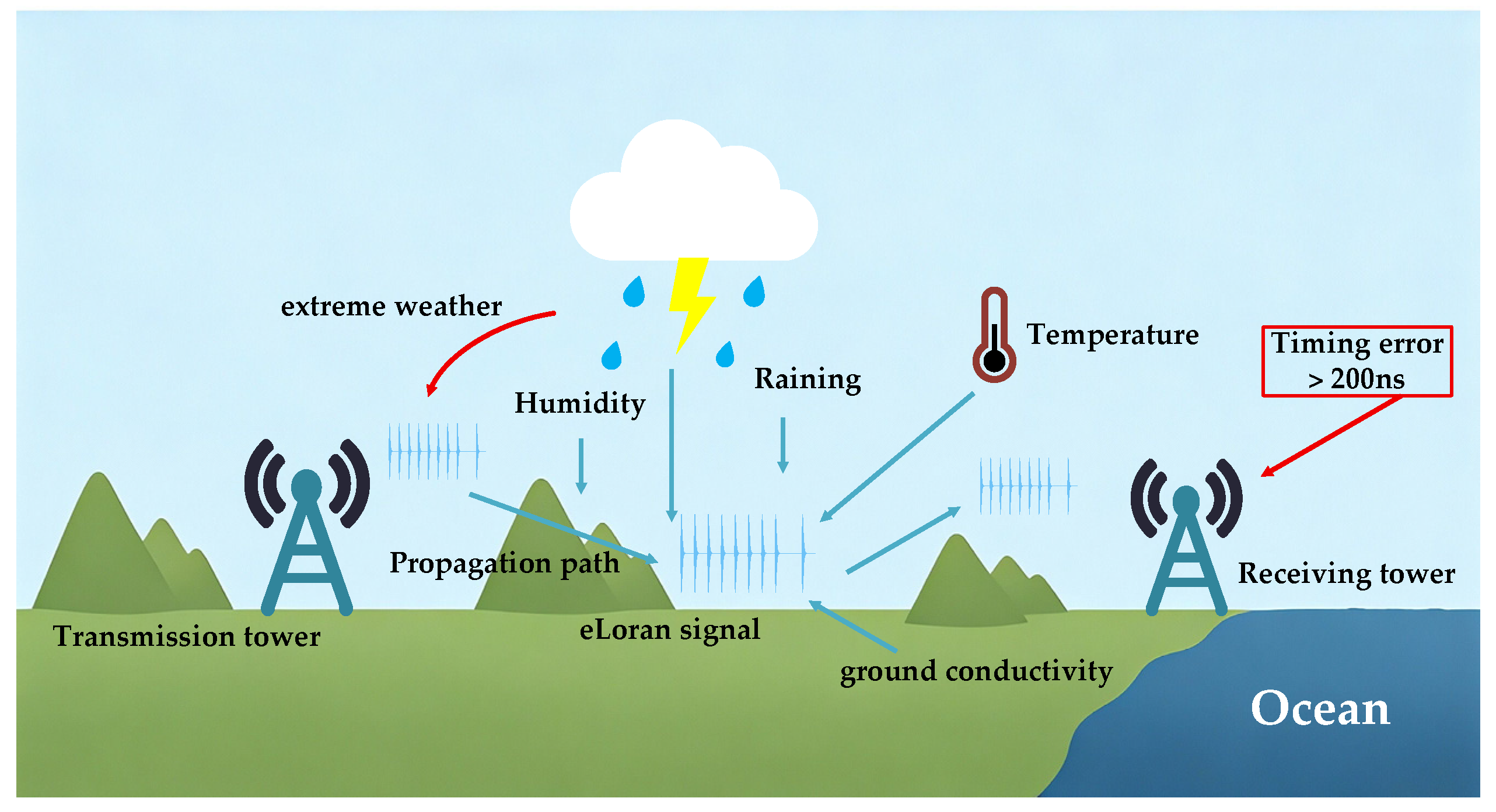
Since the eLoran system uses low-frequency ground-wave signals for timing, changes in meteorological conditions can cause the signal propagation path to shift [10]. Especially in extreme weather conditions, the timing error may exceed 200 nanoseconds, seriously affecting the normal use of users [11]. Currently, the core challenge lies in the fact that the influence of meteorological factors on the signal propagation delay has a highly complex and nonlinear nature. The signal propagation parameters are affected by multiple interrelated and coupled meteorological factors, making it impossible to accurately establish a low-frequency ground-wave signal propagation delay model and accurately estimate the propagation delay [12].

Therefore, a thorough understanding of the influence mechanism of meteorological factors on the eLoran system and the establishment of a signal propagation delay prediction model based on meteorological data are powerful means to currently suppress non-systemic interference caused by meteorological factors and improve the timing accuracy of the eLoran system [11,13]. When the propagation delay data has large errors or cannot be received, this model can be used to monitor and correct the data, improve the service quality of the eLoran system, provide users with more reliable PNT guarantees, and thereby further support its wide application in key fields such as transportation, low-altitude economy, and infrastructure construction. With the development of artificial intelligence (AI) technology, actual engineering problems that were difficult to express using traditional models in previous studies and scientific research have all incorporated new models based on AI. AI, with its powerful nonlinear fitting ability and data mining capabilities, provides new solutions and schemes for multiple complex systems. At the same time, the high-precision ground-based timing system has accumulated a large amount of reliable delay observation data, and the meteorological data collection technology has become increasingly mature [14,15,16]. Together, they have laid a solid data foundation for the application of AI to build prediction models [17].

In this context, the artificial intelligence modeling methods represented by neural networks continue to develop and make significant progress, which provides an efficient and feasible technical path for the correction and prediction of eLoran signal propagation delay. Related research has gradually progressed from basic modeling to high-precision, multi-factor, and scene-based. Xu et al. took the lead in carrying out related research in 2006, and used BPNN to establish an additional second-time-delay factor (ASF) correction model, and realized the accuracy compensation of microsecond level for the first time, which laid a foundation for the subsequent research on time delay correction based on neural network [18]. On this basis, Yang’s team thoroughly explored the association law between meteorological factors and time delay through many experiments in 2017, revealing the synchronization between diurnal temperature variation and long-wave propagation time delay. At the same time, it was found that rainfall would cause a significant decrease in time delay. This research result provides an important theoretical basis for the subsequent integration of multiple meteorological factors into the modeling [19]. In response to the issue that the short-distance propagation delay is affected by the time-varying meteorological factors, Xi’s team further optimized the modeling approach in 2019 and constructed a BPNN model with multiple meteorological factors. Compared with the traditional single-factor least squares model, the accuracy was significantly improved, and the technical framework of multi-factor collaborative modeling was perfected [20]. Based on this multi-factor modeling foundation, Wang et al. continued to deepen their research and proposed a BPNN-ASF correction model that integrates multiple parameters such as earth conductivity, atmospheric refractive index, temperature, and humidity. This model reduced the correction error to within 190 ns, further enhancing the correction accuracy of the model [21]. Meanwhile, Wang Lili’s team proposed a least squares time-varying model based on long-term monitoring data, providing a different technical approach for time delay correction [22]. As the research progressed, the modeling methods became increasingly diverse, and the model accuracy continued to improve. In 2021, Pu’s team innovatively adopted the generalized regression neural network (GRNN) and proposed a prediction method that integrates multiple meteorological factors, reducing the prediction error to the order of 23 ns, achieving a significant improvement in the accuracy of delay prediction [23]. In 2023, Liu Shiyao, based on the modeling of multiple meteorological factors, further expanded the modeling scope and proposed a BPNN model that integrates meteorological factors from multiple regions. Its performance was significantly superior to that of traditional linear and simple neural network models, enriching the modeling schemes in multiple scenarios [11]. In 2025, in response to the problem of time delay fluctuations caused by meteorological fluctuations in the long-distance transmission scenario of eLoran signals, our team proposed a targeted method based on path-weighted Pearson correlation analysis and a BPNN prediction model. This effectively achieved precise prediction of the propagation time delay of eLoran signals in the long-distance transmission scenario, further improving the modeling technology for long-distance scenarios [17]. At the same time, Di et al. focused on the actual needs of resource-constrained scenarios and proposed a dynamic weighted (DW) model that dynamically adjusts the weights of the long short-term memory neural network (LSTM) and the random forest (RF). This model takes into account both the highest prediction accuracy and the optimal computational efficiency, providing a practical solution for real-time navigation prediction [24]. In addition, Kang et al. combined meteorological data with terrain elevation to construct a machine learning model for estimating the propagation delay of eLoran, further improving the timing accuracy of eLoran as a supplementary PNT system. The above research was progressive and focused on different aspects, respectively improving the theoretical system and technical path for correcting and predicting the signal propagation delay of eLoran in terms of modeling methods, influencing factors, and scene adaptation, laying a solid theoretical foundation and practical reference for this study [25].

From the research progress, although artificial intelligence methods have been widely applied and achieved results in the problem of predicting the propagation delay of eLoran signals, their universality and optimality still need to be further explored when dealing with the complex task of predicting the propagation delay of eLoran signals, which involves high-dimensional, nonlinear, and spatiotemporal coupled meteorological-delay relationships. Using different methods to preprocess the input data has a significant impact on the prediction results of the model. Moreover, the performance of different types of models may show significant differences. Currently, there is a lack of systematic comparative studies on multiple models in predicting the propagation delay of eLoran signals using a unified high-quality dataset, and no optimization is conducted. Such systematic comparative research not only helps to select the optimal model for actual system deployment, but also to thoroughly understand the differences in physical mechanisms revealed by different models, providing new directions for future hybrid model design or model optimization innovation.

To fill the gaps in the research, the main contributions of this paper are as follows.

Firstly, for the first time, on a unified high-quality dataset, the performance of various representative models (including traditional machine learning, deep learning models, and neural network models) in predicting the long-distance propagation delay of eLoran signals was systematically compared and evaluated, providing a basis for subsequent model selection and optimization.

Secondly, the feasibility of the meteorological factor algorithm based on path weighting and the use of path propagation delay data to predict the propagation delay data of the target reference station was verified. An eLoran signal propagation delay prediction model that integrates the meteorological factor data weighted by paths and the path propagation delay data was proposed, which enhanced the prediction accuracy of the model for the propagation delay of the eLoran signal.

Finally, based on the model evaluation results and the data optimization plan, a highly accurate propagation delay prediction method was established. This effectively suppressed the propagation delay errors caused by meteorological fluctuations and improved the timing reliability of eLoran in extreme weather conditions. It provides reliable PNT services for low-altitude aircraft in complex weather environments, which is a key fundamental technical support for the safe and efficient operation of low-altitude aircraft.

2. Materials and Methods

In the first chapter, the core issues of eLoran signal propagation delay in long-distance scenarios are proposed, such as the nonlinear influence of meteorological factors and the lack of comparison of multi-model systems in existing studies. This chapter will elaborate on the materials and methods to achieve high-precision time delay prediction. After that, the data are processed, and the validity of the path weighting and differential station data prediction theory is verified, and a variety of models are constructed by combining the four prediction tasks to provide solid support for the subsequent experimental results analysis and optimal model screening.

2.1. Theoretical Basis and Model Algorithm

2.1.1. eLoran Signal System and Sources of Timing Error Fluctuation

The eLoran system is an enhanced version of the Loran-C system, incorporating data modulation, new antenna radiation elements, and fully solid-state transmitters. Its central frequency is 100 kHz, and the bandwidth is 20 kHz. In the spectrum allocation chart of the International Telecommunication Union (ITU), the eLoran signal is a long-wave signal with a standard pulse rise edge [10,26]. The eLoran signal is transmitted in the form of pulse groups, using tri-state pulse position modulation technology or ninth pulse modulation technology to modulate the time information in each pulse. The signal is broadcast via long-wave antennas to users nationwide. Users receive the eLoran signal through an eLoran signal receiver, detecting the standard zero-crossing point 30 μs after the pulse start as the phase tracking point. The receiving device processes and demodulates the received eLoran signal to obtain relevant time information, thereby achieving the timing function. The single pulse form of the eLoran signal is Formula (1):

$$s\left(t\right)=\left\{\begin{array}{c}A{\left({\displaystyle \frac{t-\tau }{t_p}}\right)}^2\mathrm{e}\mathrm{x}\mathrm{p}\left(2-2{\displaystyle \frac{t-\tau }{t_p}}\right)\sin \left(2\pi f_{0}t+P_c\right), \hspace{1em}\hspace{1em}\tau \le t\le t_p+\tau \\ 0 , t<\tau \end{array}\right.$$

(1)

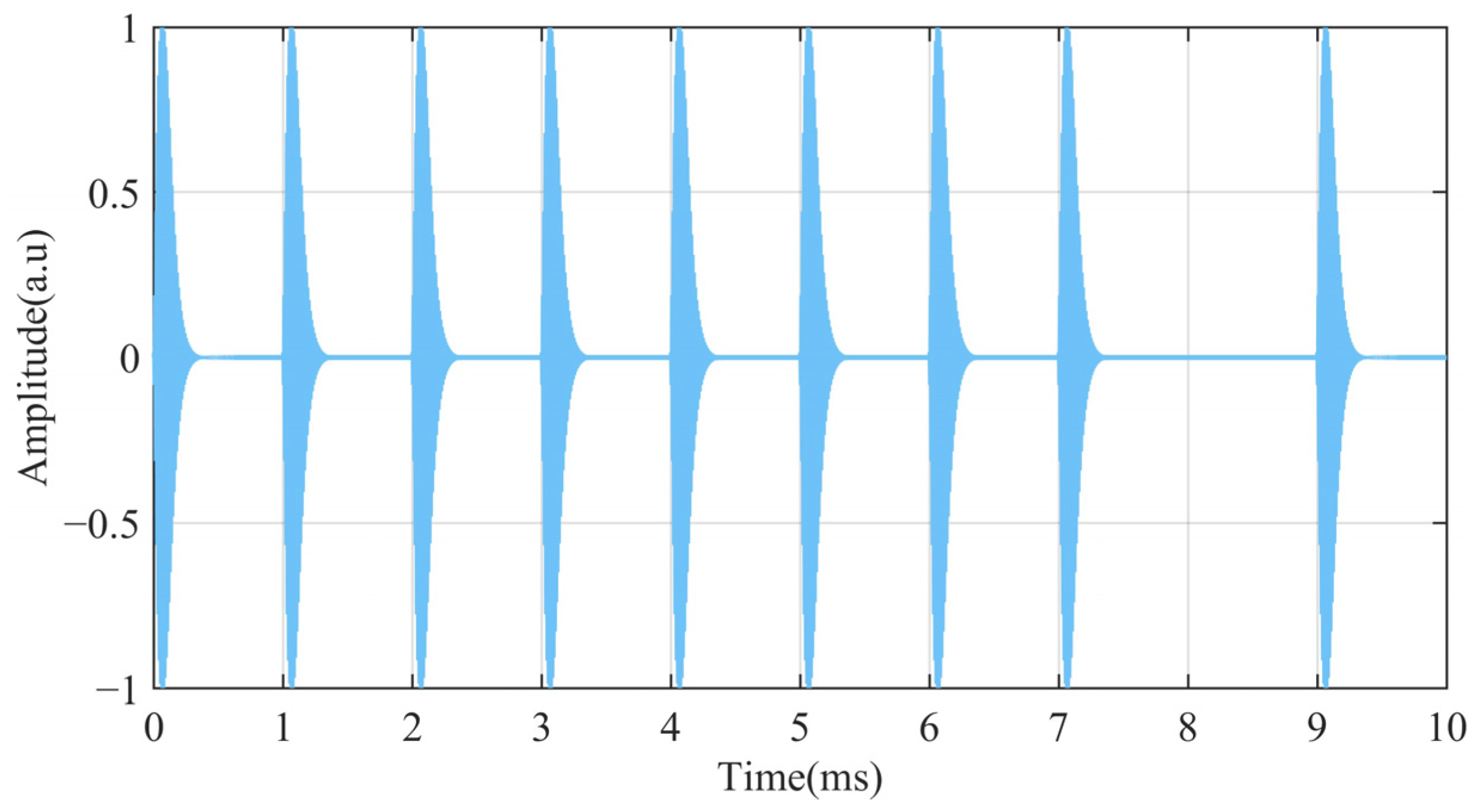
where $A$ is the amplitude parameter; $\tau$ is the envelope period difference; $f_0$ is the carrier frequency of 100 kHz; $P_c$ is the phase encoding, which takes 0 or π; and $t$ is the time in μs. Figure 1 shows the pulse group structure of the main transmitting station of the eLoran signal. The main transmitting station signal group is 9 pulses; the first 8 pulses are separated by 1 ms, the 9th pulse is separated by 2 ms, and the 3–8 pulses use the three-state pulse position modulation (PPM) technology to modulate the time information [27]. The six pulse groups are subjected to pulse position modulation with three states of time modulation values of 0 or ±1 μs to carry time information. The modulated information is encoded using Read-Solomon (RS) and Cyclical Redundancy Check (CRC) coding techniques. During transmission, the signals are broadcast according to a specific Group Repetition Interval (GRI) and the three-state pulse modulation method. GRI refers to the time interval between two adjacent pulse group signals transmitted by the same broadcasting station, and each broadcasting station has a uniquely determined GRI. Upon signal reception, the transmitting station can be identified by judging the GRI, and the received multi-pulse group signals are demodulated and decoded to obtain the time information.

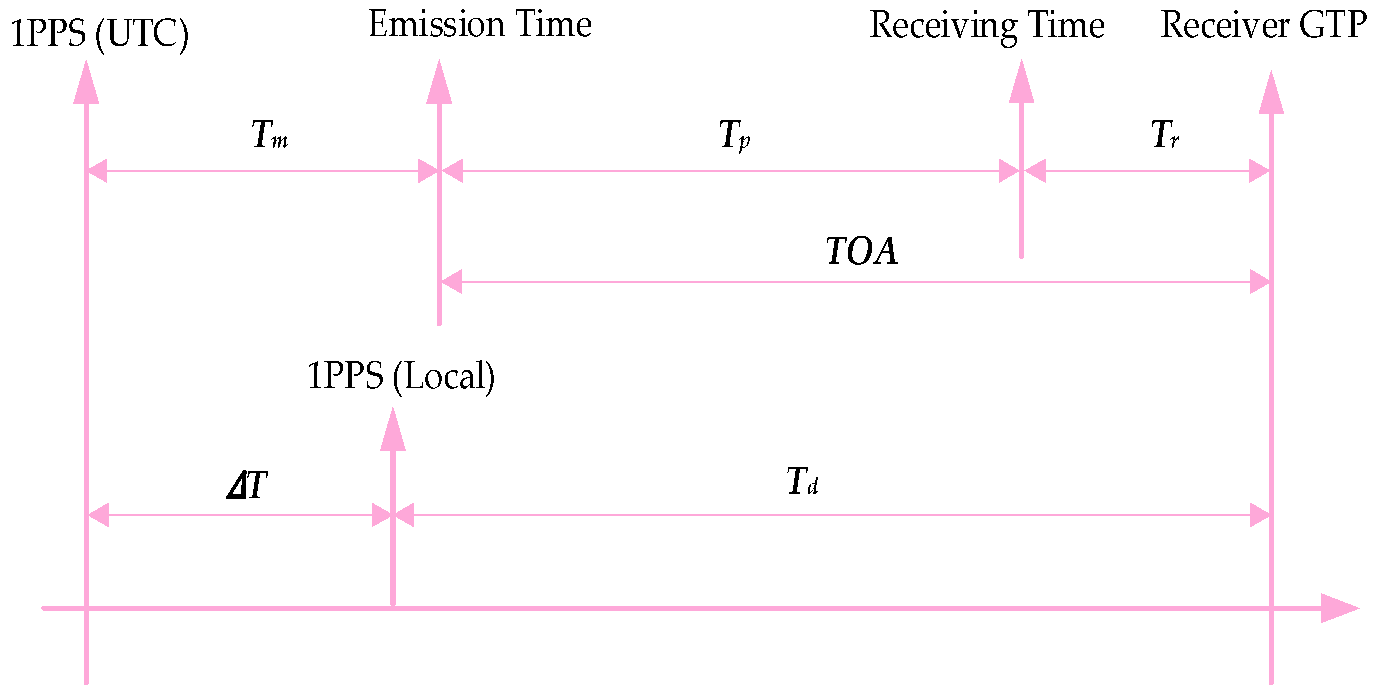
The timing principle of the eLoran signal at the user end is to calibrate the user’s local time by using the received eLoran signal carrying standard time information, and the calculation formula is Formula (2):

$$\Delta T=T_m+TOA-T_d=T_m+T_p+T_r-T_d$$

(2)

where $\Delta T$ represents the time difference between the local user time and the standard time, which is the core calculation result in the time service process. By calculating this parameter, the user’s local time is updated with the time information obtained by decoding and the result, and a time service process is completed. $T_m$ is the time difference between the transmitted signal and the standard time signal, which can be obtained from the demodulation time code information. $T_p$ is the absolute delay of signal propagation in the wireless channel, which is uncertain. It is the core parameter that users pay attention to in the timing process, and it is also an important variable that affects the timing accuracy. $T_r$ is the overall delay of the relevant receiving device, which can be obtained by calibration and is usually a fixed value. $T_d$ is the time deviation between the receiver’s internal 1Pulse Per Second (PPS) signal and the receiver Group Trigger Pulse (GTP) signal can also be measured by the internal counter of the receiver. The GTP time corresponds to the standard zero crossing of the first pulse signal of the eLoran pulse group. Through the period identification process, the eLoran receiver determines the GTP time and tracks the phase of the standard zero-crossing point; then, it accurately measures the time of arrival (TOA) of the ground-wave signal and finally realizes the timing and position service functions. In summary, except $T_p$, the other parameters can be accurately obtained by known methods or equipment. Therefore, the most important thing when using the eLoran signal for timing is to accurately estimate the absolute time delay $T_p$ in the process of the eLoran signal from the transmitting antenna, through the transmission channel, and then to the receiving antenna, the premise of the eLoran signal is that it can accurately transmit time signals. Figure 2 shows the timing method for eLoran signal reception [17,28].

$T_p$ consists of three parts: the primary time-delay factor ($PF$), the second time-delay factor ($SF$), and $ASF$. The definitions of the three are as follows: the $PF$ is defined as the propagation time of the signal from the transmitting antenna to the receiving antenna in the ideal infinite uniform air medium. Both $SF$ and $ASF$ represent the additional effects of the ground and sea media on the propagation delay of eLoran signals, but their subdivision mechanisms are different: the $SF$ is the additional delay caused by the seawater medium alone, and the $ASF$ is the additional propagation delay caused by the difference in the conductivity of the land medium and the sea medium when the signal propagates across the land medium and the sea medium, and the mathematical expression is Formula (3):

$$T_p=PF+SF+ASF={\displaystyle \frac{\int n_{s}dS}{c}}+{\displaystyle \frac{{10}^6}{\omega }}argW\left(f,d,\epsilon ,\sigma \right)$$

(3)

where $S$ represents the signal propagation distance, calculated using the great circle distance calculation formula, $n_s$ represents the atmospheric refraction index on the path through which the signal passes, and $c$ is the speed of light in vacuum. $\omega$ is the center angular frequency of the eLoran signal, $W$ is the equivalent attenuation function, $f$ is the signal propagation frequency, $\epsilon$ is the ground permittivity, and $\sigma$ is the ground equivalent conductivity of $f$ frequency signal propagation [29,30,31,32,33]. Based on the existing research in the paper [11,17], it can be known that in the calculation of propagation delay, not only will the atmospheric refractive index $n_s$ fluctuate due to meteorological factors, but the ground equivalent conductivity will also exhibit significant seasonal and diurnal variations with changes in temperature and humidity. For the same location, when there is heavy precipitation or a sudden change in surface temperature, the temperature and humidity changes in the soil cause fluctuations in the soil’s conductivity characteristics, resulting in fluctuations in $ASF$, and ultimately manifesting in the fluctuation of the absolute propagation delay $T_p$. Sometimes, the propagation delay fluctuation error can reach the order of hundreds of nanoseconds.

Figure 3 shows the schematic of the influence of meteorological factors on the propagation delay of eLoran signals.

2.1.2. Introduction of Propagation Delay Prediction Model Algorithm

Combined with the characteristics of the research data, the application scenarios of the algorithm, and the actual operation requirements of the eLoran system, this study determines the algorithm subset from the three key dimensions of computational complexity, algorithm coverage, and model stability. The selection basis is as follows: considering that the scale of experimental data has not yet reached the adaptation conditions of high-complexity algorithms at this stage, blindly adopting complex algorithms will not only cause a large consumption of computing power resources, but also the improvement of algorithm performance is very limited, which makes it difficult to reflect the practical application value. Therefore, high-complexity algorithms are not included in the scope of research. The selected algorithm subset includes classical machine learning algorithms such as support vector machine and random forest. At the same time, the linear model is introduced to carry out regression comparison experiments, which can fully cover the mainstream regression algorithm types in related research fields and ensure the comprehensiveness, representativeness, and scientific validity of algorithm comparison experiments. In addition, the operational stability of high-complexity models is generally less than that of classical algorithms. As the core backup system of the eLoran system, stability is a key factor in realizing its function. To make the prediction model fit the actual application requirements of the eLoran system, this study preferentially selects the classical algorithm with better operation stability to construct the prediction model.

In this paper, the meteorological factor data on the path and the propagation delay data of the differential reference station on the path are used. And ridge regression (RR) [34], random forest [35], support vector regression (SVR) [36], Gaussian kernel regression (GKR) [37], back propagation neural network [38], generalized regression neural network [39], long short-term memory neural network [40], convolutional neural network–long short-term memory neural network (CNN-LSTM) [41] and other models to establish the propagation delay prediction model of the target differential reference station. The models used in this study cover linear models (LMs), traditional machine learning models (MLs), and deep learning and neural network models (DLs and NNs). The relevant descriptions of the models used in this paper are shown in

Table 1. Description of the modeling approach adopted in this paper [34,35,36,37,38,39,40,41].

Type	Model	Description	Hyperparameters	Advantages	Disadvantages
LM	RR	The L2 regularization term is introduced into the least squares estimation method to improve the numerical stability and calculation accuracy of the regression coefficients by sacrificing unbiasedness.	Regularization strength	The coefficient estimation is stable and simple to calculate	This leads to a biased estimation of the coefficient; variable selection cannot be performed
ML	RF	The ensemble learning algorithm based on decision trees constructs multiple decision trees by sampling the original data with replacement, and then reduces the risk of overfitting of a single decision tree by voting or averaging the results.	The number of decision trees, the maximum depth of each tree, the maximum number of features to consider when splitting, and the minimum number of leaf samples	Strong robustness and ability to handle high-dimensional data	Poor interpretability and high computational cost
	SVR	Based on the insensitive function and kernel function, the data is mapped to a high-dimensional space, and the flat prediction function is determined to make most of the data fall within the allowable range of prediction error.	Penalty coefficient, kernel function type, insensitive band width, and kernel function parameter	Can deal with nonlinear high-dimensional problems	Large-scale data is slow to train, sensitive to hyperparameters, and has poor interpretability
	GKR	The Gaussian kernel function is used to measure the similarity between the input samples and the training samples, and the predicted value is obtained by a weighted summation of the similarity.	Kernel width and regularization coefficient	No assumptions about the data distribution; the local features are captured well	Sensitive to hyperparameters; low computational efficiency
DL&NN	BPNN	In the forward propagation stage, the input signal was transmitted to the hidden layer and the output layer through the weight matrix, and the activation function was used to realize the nonlinear transformation. In the back propagation stage, the chain rule is used to calculate the error gradient of the parameters of each layer, and the weights and biases are updated according to the principle of gradient descent.	Number of hidden layers, number of neurons, learning rate, activation function, number of iterations, and batch size	Adaptable to complex data relationships; learns features adaptively	Easy to overfit; slow convergence
	GRNN	It is assumed that the input variables and output variables obey the joint probability density function, and the density function is estimated through the training samples.	Smoothness factor	Fast training speed; excellent nonlinear fitting ability	Low efficiency under large-scale data
	LSTM	The gated mechanism is used to solve the problem of gradient disappearance or explosion of the recurrent neural network, which can effectively capture the dependencies in long sequence data.	Number of hidden layer neurons, learning rate, sequence length, discard rate, number of iterations, and batch size	The fitting effect of the time series data is excellent	The structure is complex, the training speed is slow, and the computational cost is high
	CNN-LSTM	CNN: The convolution kernel sliding and pooling operation were used to extract the local spatial features of the data and reduce the data dimension. LSTM: It takes the feature sequence output by CNN as input to capture the time dependence between features. These enable end-to-end learning of spatiotemporal data.	Hyperparameters for CNN and LSTM	It captures both spatial features and temporal dependence, which is suitable for spatiotemporal fusion tasks	Complex structure; hyperparameter tuning is difficult; it is easy to overfit small data

.

There are many modeling methods for data regression prediction. Due to the space limitation of this paper, this paper only lists some common data regression prediction methods. We can use these methods to establish the corresponding propagation delay prediction model, as well as use different data construction methods to complete the corresponding prediction tasks and compare them.

2.2. Data Acquisition and Processing Methods

2.2.1. Data Acquisition

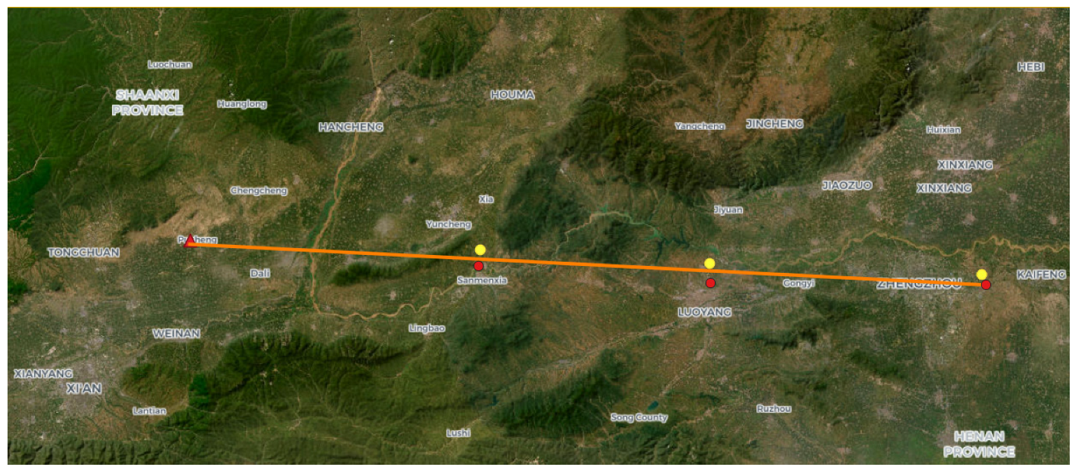
In this study, multi-source data were comprehensively used for analysis. The eLoran signal propagation delay data were derived from the eLoran signal transmitted by the BPL long-wave time service station in Pucheng County, Weinan City, Shaanxi Province, China. The data is transmitted through an eLoran signal long-wave timing receiver (KTL-202A-F, Xi’an Air-space Electronic technology Co., Ltd., Xi’An, China; The equipment was sourced from Xi’An Air-space Electronic technology Co., Ltd.), long-wave receiving antenna (KTL-606B-DF14, Xi’an Air-space Electronic technology Co., Ltd., Xi’an, China; The equipment was sourced from Xi’an Air-space Electronic technology.Co., Ltd.), high-precision GNSS timing receiver (IME-GNSS200T-2, Xi’an Air-space Electronic technology Co., Ltd., Xi’an, China; The equipment was sourced from Xi’an Air-space Electronic technology Co., Ltd.), GNSS receiving antenna, and time interval counter (MTIM712, Xi’an Air-space Electronic technology Co., Ltd., Xi’an, China; The equipment was sourced from Xi’an Air-space Electronic technology Co., Ltd.), among other equipment. Three differential reference stations in Sanmenxia, Luoyang and Zhengzhou were collected from 12 October 2024 to 1 January 2025. The collection duration was 82 days, the valid data duration was 67 days, and the data acquisition resolution was once per second. Meteorological data are from the data center of China Meteorological Administration, collected from four national weather stations in Pucheng, Sanmenxia, Luoyang and Zhengzhou. The collection period is from 1 October 2024 to 8 January 2025, with a total of 100 days. The valid data duration is 67 days, and the data resolution is 1 time per minute. It covers temperature, relative humidity, saturated vapor pressure, precipitation, vapor pressure, ground temperature, average wind direction, average wind speed, visibility and other types. Due to the relevant safety regulations of meteorological data, the acquisition equipment and specific details are not disclosed in the paper. Path data were calculated by computer based on the actual coordinates of the BPL long-wave timing station in Pucheng and differential reference stations in Sanmenxia, Luoyang and Zhengzhou, with reference to [39].

Figure 4 shows the relative spatial positions and correspondences of the differential stations and weather stations along the path described by the above data from the BPL longwave time service station in Pucheng to the differential reference station in Zhengzhou, where the yellow dot represents the relative position of each meteorological observation station, the red triangleis the BPL longwave time service station in Pucheng, and the red dot represents the position of each differential reference station. The orange solid lines represent the schematic diagram of the propagation path.

2.2.2. Data Processing Methods

The raw data collected above is processed through the following steps:

• Data cleaning

The overall goal of data cleaning is to eliminate the outliers in the original data (propagation delay data, meteorological data), fill the missing data, discard the invalid data that cannot be repaired, ensure the integrity, accuracy and effectiveness of the data, lay a foundation for subsequent data smoothing, down-sampling, time alignment and normalization processing, and ensure the reliability of subsequent model input data.

(a) Review and complete the data

Specific role: Solve the problem of missing and discontinuous sampling in the original data, avoid the interference of missing data and discontinuous data on the subsequent processing results, ensure the integrity of the data, and provide complete basic data for the elimination of outliers and subsequent steps.

Specific operations: Firstly, for the propagation delay data, it checked whether the number of sampling points per day met 86,400, and whether the data collection time was continuous. For the missing data, according to the noise of the correct data in the previous period, the change trend of the correct data before and after was combined to complete the missing data. If the amount of data missing on a day is too large to restore the validity of the data by completion, the propagation delay data of that day will be discarded. For meteorological data, the same continuity and integrity verification criteria were used to check whether the number of sampling points per day met 1440 and whether the collection time was continuous. Because the meteorological data has the characteristics of stable change and no mutation, the linear interpolation method was used to complete the missing data. If the missing amount of meteorological data on a given day is too large, the meteorological data of that day is also discarded.

(b) Remove outliers

Specific functions: eliminate extreme values and abnormal fluctuation data existing in the original data, avoid abnormal data distorting the change trend of the data itself, ensure the accuracy of the data, and reduce the negative impact of abnormal values on subsequent data processing and model training.

2.

Specific operation: the method of combining the 3σ rule with the soft and hard threshold was adopted, and the outliers were removed from the completed propagation delay data and meteorological data. The specific steps are as follows: Take 10 min as a time window, and calculate the standard deviation of the data in the previous 10 min corresponding to each data point to be detected; according to the 3σ rule, the value of the point to be detected is compared with 3 times the standard deviation of the data in the first 10 min. If the value of the point exceeds this range, it is determined to be an outlier value, and it needs to be removed. Set double thresholds for auxiliary screening: the first is the threshold of the number of continuous repair data, which is used to deal with large-scale continuous data anomalies. If a certain segment of data has large-scale continuous anomalies and the number of continuous repairs exceeds the set threshold, this segment of data will be discarded. The other is the threshold of data extreme value, which directly eliminates the extreme outliers beyond the reasonable range, and uses the average value of the data 10 min before the point to add the corresponding noise value for replacement repair. Carry out smoothing and down-sampling.

Specific functions: remove all kinds of noise carried in the propagation delay data, and restore the real change trend of the data itself. The sampling resolution of time delay data and meteorological data was unified to reduce data redundancy and improve the efficiency of subsequent data processing. At the same time, the sampling frequency matching of the two types of data was ensured to facilitate subsequent time alignment.

Specific operation: For the propagation delay data, due to all kinds of noise in the collection process, there are invalid fluctuations in the data. The average filtering method is used to remove noise. After many experiments, the optimal filtering window size is determined as 1800 sampling points, which can remove the noise to the greatest extent and restore the real change trend of propagation delay data clearly. Considering that the sampling resolution of propagation delay data is one point in one second, while the sampling resolution of meteorological data is one point in one minute, and the sampling frequency difference between them is large, the propagation delay data is down-sampled, and the down-sampling rate is set to 60, and the sampling resolution of propagation delay data is adjusted to one point in one minute, which is consistent with the sampling resolution of meteorological data.

3.

Align the time scales

Specific functions: to solve the problems of inconsistent timestamps between propagation delay data and meteorological data, and the time mismatch caused by early rejection of some data, to ensure that the two types of data are strictly corresponding in the time dimension, and to provide a time-unified data basis for subsequent data fusion and model input.

Specific operations: Firstly, the problem of time stamp time zone difference was solved: UTC time stamp was used in the propagation delay data collection, while Beijing time stamp was used in the meteorological data collection, and there was a time difference of 8 h between the two. The UTC time stamp of the propagation delay data was adjusted to the Beijing time stamp to realize the unification of time zones. Secondly, for part of the propagation delay data and meteorological data discarded in the first step of data cleaning, another type of data in the corresponding time range was discarded synchronously, that is, when the propagation delay data at a certain time was discarded, the meteorological data corresponding to the time was discarded synchronously, and vice versa, to ensure that the time range of the two types of data was completely consistent and the timestamps were strictly aligned.

4.

Normalization

Specific functions: eliminate the numerical differences caused by different dimensions between propagation delay data and various types of meteorological data, avoid the imbalance of model weight distribution caused by dimension differences, make all types of data in the same order of magnitude, and improve the convergence speed and training effect of subsequent model training.

Specific operations: Before the data was input into the model, the z-score method was used to normalize the propagation delay data and various meteorological data. After normalization, all the data meet the statistical characteristics of a mean of 0 and a standard deviation of 1, which ensures that the dimensions of all kinds of data are unified. The normalization formula is given in Formula (4):

$$\mathrm{y}={\displaystyle \frac{\mathrm{x}-\mu }{\sigma }}$$

(4)

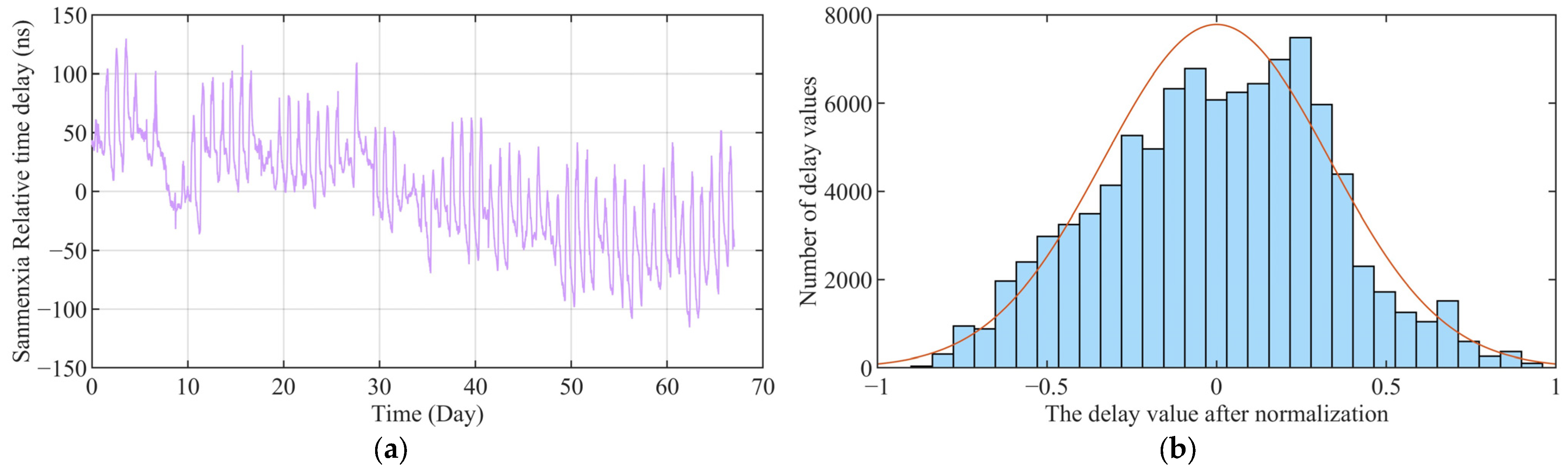
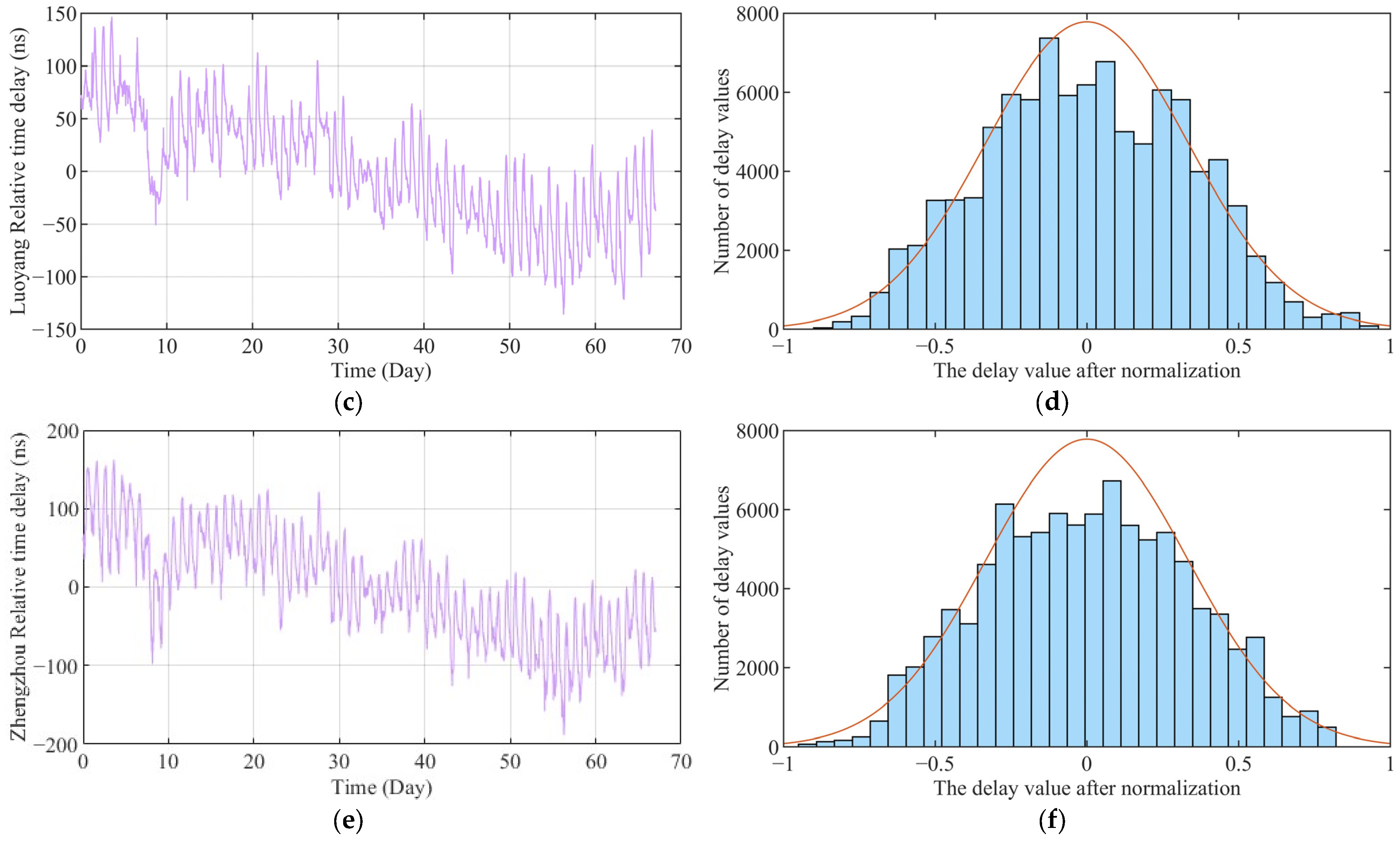
where $\mathrm{x}$ is the original data, $\mu$ is the mean of the whole data, $\sigma$ is the standard deviation of the whole data set, $\mathrm{y}$ is the data after normalization, Figure 5 is the curve of the propagation delay change after processing, and the distribution histogram of the propagation delay data after normalization.

2.3. Path-Related Analysis Method

According to the theory proposed by literature [14,21], in the long-distance transmission scenario, the meteorological conditions on the path are complex and changeable, so it is one-sided to analyze the correlation between propagation delay and meteorological factors by only using the single meteorological data of the receiving weather station on the path. Literature [21] proposes the Pearson correlation coefficient analysis method based on path weighting. By analyzing the measured data using this weighting method, it is verified that the method is effective in analyzing the short-term propagation delay. However, the literature does not analyze the long-term delay, nor does it consider whether the propagation delay data obtained by the differential reference station on the path can help to improve the propagation delay estimation accuracy of the target differential reference station. The related research in this paper complements the shortcomings in the above literature research and proposes a method to improve the propagation delay prediction accuracy of the target differential reference station by using the propagation delay data of the differential reference station on the path. At the same time, it is analyzed from the theoretical point of view and verified by using the measured data.

2.3.1. Theoretical Basis for Correlation Analysis of Propagation Delay Data

eLoran signal propagation is affected by meteorological factors, resulting in changes in signal propagation speed and delay. These changes are mainly reflected in the SF and ASF of the propagation delay. Considering that the eLoran signal is transmitted from the BPL longwave time service station in Pucheng (point A), the signal arrives at the receiver of the differential reference station in Luoyang (point B) and the receiver of the differential reference station in Zhengzhou (point C) respectively. On this propagation path, we consider that the sum of the quadratic delay and the additional quadratic delay of the two paths are $\Delta {\tau }_B$ and $\Delta {\tau }_C$, respectively. If most of the path points A to point B and point A to point C overlap and pass through the middle point D, then:

$$\Delta {\tau }_B={\displaystyle \frac{{10}^6}{\omega }}\left({\int }_A^{D}argW\left(f,\epsilon ,\sigma \right)dS+{\int }_D^{B}argW\left(f,\epsilon ,\sigma \right)dS\right)$$

(5)

$$\Delta {\tau }_C={\displaystyle \frac{{10}^6}{\omega }}\left({\int }_A^{D}argW\left(f,\epsilon ,\sigma \right)dS+{\int }_D^{C}argW\left(f,\epsilon ,\sigma \right)dS\right)$$

(6)

$$\Delta {\tau }_B-\Delta {\tau }_C={\displaystyle \frac{{10}^6}{\omega }}\left({\int }_D^{B}argW\left(f,\epsilon ,\sigma \right)dS-{\int }_D^{C}argW\left(f,\epsilon ,\sigma \right)dS\right)$$

(7)

If the same segment path point A to point D is much longer than the unique segment path point D to point B and point D to point C, then the value of $\Delta {\tau }_B$ and $\Delta {\tau }_C$ is mainly determined by the integral ${\int }_A^{D}argW\left(f,\epsilon ,\sigma \right)dS$ on the same path. A meteorological factor usually has the same property on the scale of tens of kilometers, that is, high spatial autocorrelation. And point B and point C are not far from point D; that is, in the short distance interval,

$${\int }_D^{B}argW\left(f,\epsilon ,\sigma \right)dS\approx {\int }_D^{C}argW\left(f,\epsilon ,\sigma \right)dS$$

(8)

Therefore, the difference on the right side of Formula (9) will be a small amount, so that $\Delta {\tau }_B\approx \Delta {\tau }_C$. That is, the SF of both and the ASF show a strong correlation. Based on the above analysis, it can be considered that the propagation delay data of the differential reference station on the path contains the meteorological information after path integration, which can be used as a predictor of the propagation delay data of the target differential station.

The research core of this paper focuses on the prediction of long-distance path propagation delay in the Loran system. Combined with the signal propagation characteristics of the Loran system and research scenarios, we define different propagation distances: Less than or equal to 70 km is defined as short distance, 70–150 km is medium distance, and more than 150 km is long distance. Through data verification, the assumptions of Equations (5)–(8) are all valid based on the medium and long-distance propagation scenario of 70–150 km, that is, the maximum applicable distance of this model is 150 km.

In addition, it can be known from literature [21] that due to the changeable meteorological factors on the long-distance propagation path of eLoran signals, the total propagation delay is comprehensively determined by the changes in meteorological factors on each path. It is not accurate to predict or calculate the total propagation delay by only using a single meteorological data point at the receiving place, and the calculation method of the Pearson correlation coefficient based on path weighting should be adopted. Please refer to [21] for the specific calculation method. The calculation method of the Kendall and Spearman correlation coefficient based on path weighting is similar to the calculation method of the weighted Pearson correlation coefficient, which will not be described here.

2.3.2. Analysis of Measured Data

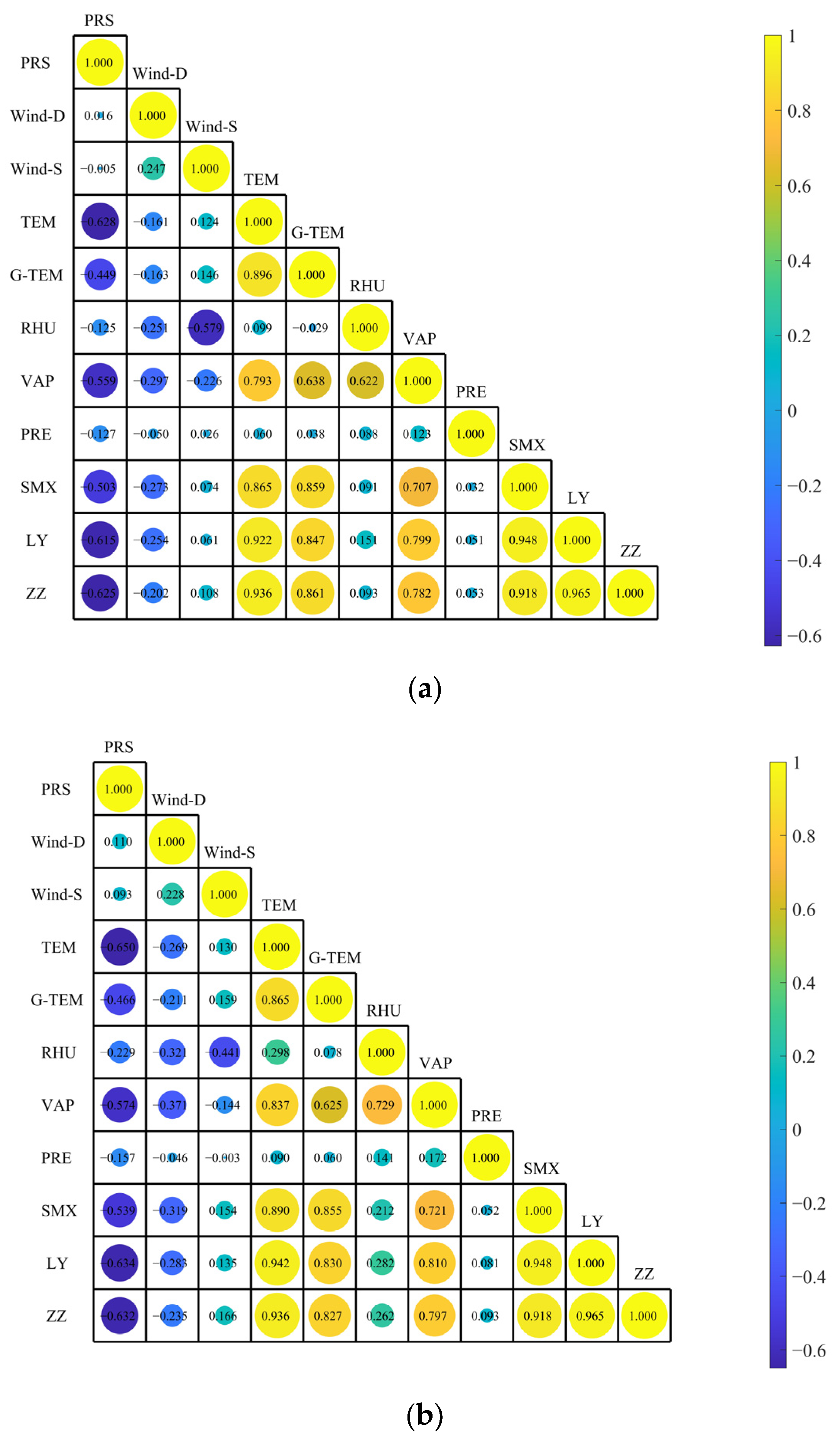
After theoretical analysis, in order to verify our conclusion, taking the Zhengzhou differential reference station as an example, the measured data of propagation delay processed above and the measured data of meteorological elements of multiple national weather stations on the path are used to calculate the long-term Pearson, Kendall and Spearman correlation coefficient matrix without path weighting and the three correlation coefficients after path weighting respectively. Due to the large amount of data, only the Pearson correlation coefficient is listed in the figure, while the other two types of correlation values that are not listed are not much different. The analysis results are detailed in Figure 6:

The size of the point in the box represents the degree of correlation; the larger the point, the higher the degree of correlation. It can be seen from the above results that the propagation time delay data of the Zhengzhou differential reference station have a strong correlation with the propagation time delay data of Sanmenxia and Luoyang differential reference stations, and the Pearson correlation coefficients are all above 0.9, indicating a strong correlation. This proves the conclusion that the propagation delay data of the differential reference station on the path can be used as a predictor of the propagation delay data of the target differential reference station. At the same time, by comparing the calculation results of the three correlation coefficients before and after weighting, it can be found that compared with the calculation results of only using the weather station data of the target location, the weighted correlation coefficient values are improved, especially the two meteorological factors of relative humidity and precipitation. Their Pearson correlation coefficients changed from unweighted 0.093 and 0.053 to weighted 0.262 and 0.093. However, the Pearson correlation coefficient of the ground temperature meteorological factor decreases after weighting, indicating that the comprehensive influence of the meteorological factor on the whole path is smaller than that only on the target site after path weighting, which reflects that the correlation coefficient calculation results based on path weighting are more scientific. At the same time, it is proven that the data after path weighting is more suitable for predicting the propagation delay of the target station.

2.4. Prediction Task Design

In order to prove that using the path weighting method for meteorological data and the propagation delay data of the differential reference station on the path can improve the prediction accuracy of the propagation delay data of the target station. At the same time, in order to compare the propagation delay prediction ability of different modeling methods for the target station under the same high-quality data set, the following four prediction tasks are designed, and the relevant data sets are constructed.

Task 1: Establish a variety of propagation delay data prediction models for the target station using a variety of meteorological factors from multiple weather stations on the path in the long-distance propagation scenario. The specific process is as follows: eight different meteorological factors, including temperature, humidity, vapor pressure, relative humidity, precipitation, wind speed, wind direction and ground temperature in Pucheng, Sanmenxia, Luoyang and Zhengzhou, without path weighting, were used as input data, and multiple prediction models covering linear models, traditional machine learning models, deep learning models and neural networks were established. It is used to predict the propagation delay data of the Zhengzhou differential reference station, and the prediction ability of the model is compared with the relevant data indicators.

Task 2: Establish a variety of propagation delay data prediction models for target stations by using multiple weather stations on the path in the long-distance propagation scenario after path weighting of a variety of meteorological factors. The specific process is as follows: The path weighting method is used to weight eight different meteorological factors, such as temperature, humidity, vapor pressure, relative humidity, precipitation, wind speed, wind direction, and ground temperature, in Pucheng, Sanmenxia, Luoyang, and Zhengzhou, respectively. The weighted meteorological factors are used as input data to establish a variety of prediction models covering linear models, traditional machine learning models, deep learning, and neural networks. It is used to predict the propagation delay data of the Zhengzhou differential reference station, and the prediction ability of the model is compared with the relevant data indicators.

Task 3: Establish a variety of propagation delay data prediction models for the target station using multiple meteorological factors of multiple weather stations on the path and propagation delay prediction data received by differential reference stations on the path in the long-distance propagation scenario. The specific process is as follows: eight different meteorological factors, such as temperature, humidity, vapor pressure, relative humidity, precipitation, wind speed, wind direction, and ground temperature, in Pucheng, Sanmenxia, Luoyang, and Zhengzhou, without path weighting, and the propagation delay data received in Sanmenxia and Luoyang, were used as the input data of the model. A variety of prediction models covering linear models, traditional machine learning models, as well as deep learning and neural networks, are established to predict the propagation delay data of the Zhengzhou differential reference station, and the prediction ability of the model is compared with the relevant data indicators.

Task 4: Establish a variety of propagation delay data prediction models for the target station by using the propagation delay prediction data received by multiple weather stations on the path after path weighting and various meteorological factors, and differential reference stations on the path in the long-distance propagation scenario. The specific process is as follows: the path weighting method is used to weight eight different meteorological factors, such as temperature, humidity, vapor pressure, relative humidity, precipitation, wind speed, wind direction, and ground temperature, in Pucheng, Sanmenxia, Luoyang, and Zhengzhou, respectively, and the propagation delay data received in Sanmenxia and Luoyang are combined as the input data of the model. A variety of prediction models covering linear models, traditional machine learning models, as well as deep learning and neural networks, are established to predict the propagation delay data of the Zhengzhou differential reference station, and the prediction ability of the model is compared with the relevant data indicators.

2.5. Model Building Method and Hyperparameter Settings

This subsection will use the eLoran signal propagation delay data from Pucheng to Zhengzhou and the corresponding meteorological data on the propagation path. The four prediction tasks described in the above subsection will be used as the basis to divide the training set, establish different eLoran signal propagation delay prediction models, and use the method of multiple experiments to set the hyperparameters of the model until the model performance reaches its best. After the best model is successfully trained, the test set data is used as the model input according to the task type to obtain the predicted value of the eLoran signal propagation delay of the Zhengzhou differential reference station, and the real value is compared and analyzed to test the performance of the best model.

2.5.1. Task 1: Unweighted Meteorological Factor Prediction Model

Firstly, eight kinds of meteorological data of 60 days are selected from the four observation points of Pucheng, Sanmenxia, Luoyang, and Zhengzhou, as the training set of model input, and the eLoran signal propagation delay data of the Zhengzhou differential reference station at the corresponding time are selected as the training set of model output. These data account for about 90% of the total data. The remaining 7 days of each data set (about 10% of the total data) were used as the test set of the model, and the optimal model was found by constantly adjusting each hyperparameter. The established optimal model and its hyperparameters are shown in

Table 2. Each optimal model and hyperparameters for task 1.

Task	Model	Input	Output	Hyperparameters
Task 1	PZNE-RR	unweighted meteorological data for Pucheng, Sanmenxia, Luoyang, and Zhengzhou	eLoran signal propagation delay data of Zhengzhou	regularization strength = 0.01
	PZNE-RF			number of decision trees = 100; type of decision tree = regression
	PZNE-SVR			kernel function type = linear; cache size = 1000 optimization routine = SMO
	PZNE-GKR			regularization term strength = auto; kernel scale parameter = auto; maximum number of optimization iterations = 1000
	PZNE-BPNN			number of hidden layers = 2; number of neurons = [16, 16], learning rate = 0.001; activation function = RELU, number of iterations = 1000; batch size = 50
	PZNE-GRNN			hyperparameters = default
	PZNE-LSTM			number of hidden = 2; layer neurons = [13, 15]; learning rate = 0.001; discard rate = 0.2; number of iterations = 4000; batch size = 50
	PZNE-CNN-LSTM			learning rate = 0.001; number of iterations = 4000; batch size = 50

. In order to facilitate the expression, RF and BPNN models are taken as examples, and the optimal parameter models in task 1 are named as: Pucheng–Zhengzhou unweighted eight-factor RF model (PZNE-RF) and Pucheng–Zhengzhou unweighted eight-factor BPNN model (PZNE-BPNN).

2.5.2. Task 2: Path-Weighted Meteorological Factor Prediction Model

Firstly, eight kinds of meteorological data of 60 days are selected from the four observation points of Pucheng, Sanmenxia, Luoyang, and Zhengzhou, and these meteorological data are path-weighted by using the path weighting method. Then, the weighted meteorological data is used as the training set of the model input, and the eLoran signal propagation delay data of the Zhengzhou differential reference station at the corresponding time is selected. As the training set of the model output, these data accounted for about 90% of the total data. The remaining 7 days of meteorological data of each meteorological data set were weighted (about 10% of the total data), and the remaining 7 days of eLoran signal propagation delay data of the Zhengzhou differential reference station were used as the test set of the model. The established optimal model and its hyperparameters are shown in

Table 3. Each optimal model and hyperparameters for task 2.

Task	Model	Input	Output	Hyperparameters
Task 2	PZWE-RR	weighted meteorological data for Pucheng, Sanmenxia, Luoyang, and Zhengzhou	eLoran signal propagation delay data of Zhengzhou	regularization strength = 0.01
	PZWE-RF			the number of decision trees = 100; type of decision tree is regression
	PZWE-SVR			kernel function type = linear; cache size = 1000 optimization routine = SMO
	PZWE-GKR			regularization term strength = auto; kernel scale parameter = auto; maximum number of optimization iterations = 1000
	PZWE-BPNN			number of hidden layers = 2; number of neurons = [16, 17], learning rate = 0.001; activation function = RELU, number of iterations = 1000; batch size = 50
	PZWE-GRNN			hyperparameters = default
	PZWE-LSTM			number of hidden = 2; layer neurons = [14, 13]; learning rate = 0.001; discard rate = 0.2; number of iterations = 4000; batch size = 50
	PZWE-CNN-LSTM			learning rate = 0.001; number of iterations = 4000; batch size = 50

. For ease of expression, the optimal parameter model in task 2 is named as: Pucheng–Zhengzhou path-weighted eight-factor RF model (PZWE-RF), Pucheng–Zhengzhou path-weighted eight-factor BPNN model (PZWE-BPNN).

2.5.3. Task 3: Unweighted Meteorological + Path Delay Prediction Model

Firstly, the 60-day meteorological data and the eLoran signal propagation delay data received by the Sanmenxia and Luoyang differential reference stations at the corresponding time are selected from the four observation points in Pucheng, Sanmenxia, Luoyang and Zhengzhou, respectively, as the training set of the model input, and the eLoran signal propagation delay data of the Zhengzhou differential reference station at the corresponding time are selected. As the training set of the model output, these data account for about 90% of the total data, and the remaining 7 days of each data set (about 10% of the total data) are used as the test set of the model. The optimal model is found by constantly adjusting each hyperparameter, and the optimal model and its hyperparameters are shown in

Table 4. Each optimal model and hyperparameters for task 3.

Task	Model	Input	Output	Hyperparameters
Task 3	PZNT-RR	unweighted meteorological data for Pucheng, Sanmenxia, Luoyang, and Zhengzhou, and eLoran signal propagation delay data for Sanmenxia and Luoyang	eLoran signal propagation delay data of Zhengzhou	regularization strength = 0.01
	PZNT-RF			the number of decision trees = 100; Type of decision tree is regression
	PZNT-SVR			kernel function type = linear; cache size = 1000 optimization routine = SMO
	PZNT-GKR			regularization term strength = auto; kernel scale parameter = auto; maximum number of optimization iterations = 1000
	PZNT-BPNN			number of hidden layers = 2; number of neurons = [15, 14], learning rate = 0.001; activation function = RELU, number of iterations = 1000; batch size = 50
	PZNT-GRNN			hyperparameters = default
	PZNT-LSTM			number of hidden = 2; layer neurons = [14, 14]; learning rate = 0.001; discard rate = 0.2; number of iterations = 4000; batch size = 50
	PZNT-CNN-LSTM			learning rate = 0.001; number of iterations = 4000; batch size = 50

. For ease of presentation, the optimal parameter models in task 3 are named as: Pucheng–Zhengzhou unweighted ten-factor RF Model (PZNT-RF), Pucheng–Zhengzhou unweighted ten-factor BPNN model (PZNT-BPNN).

2.5.4. Task 4: Weighted Meteorological + Path Delay Prediction Model

Firstly, 60 days of meteorological data are selected from the four observation points of Pucheng, Sanmenxia, Luoyang, and Zhengzhou, respectively, and these meteorological data are weighted by using the path weighting method. The eLoran signal propagation delay data received by Sanmenxia and Luoyang differential reference stations at the same time are selected. The eLoran signal propagation delay data of the Zhengzhou differential reference station at the corresponding time is selected as the training set of the model output, which accounts for about 90% of the total data. The remaining 7 days of meteorological data are weighted, combined with the remaining 7 days of propagation delay data (about 10% of the total data), as the input data of the model test set. The eLoran signal propagation delay data of the Zhengzhou differential reference station for the remaining 7 days were used as the output data of the model test set, and the optimal model was found by constantly adjusting each hyperparameter. The established optimal model and its hyperparameters are shown in

Table 5. Each optimal model and hyperparameters for task 4.

Task	Model	Input	Output	Hyperparameters
Task 4	PZWT-RR	weighted meteorological data for Pucheng, Sanmenxia, Luoyang, and Zhengzhou and eLoran signal propagation delay data for Sanmenxia, Luoyang	eLoran signal propagation delay data of Zhengzhou	regularization strength = 0.01
	PZWT-RF			the number of decision trees = 100; Type of decision tree is regression
	PZWT-SVR			kernel function type = linear; cache size = 1000 optimization routine = SMO
	PZWT-GKR			regularization term strength = auto; kernel scale parameter = auto; maximum number of optimization iterations = 1000
	PZWT-BPNN			number of hidden layers = 2; number of neurons = [17, 16], learning rate = 0.001; activation function = RELU, number of iterations = 1000; batch size = 50
	PZWT-GRNN			hyperparameters = default
	PZWT-LSTM			number of hidden = 2; layer neurons = [16, 16]; learning rate = 0.001; discard rate = 0.2; number of iterations = 4000; batch size = 50
	PZWT-CNN-LSTM			learning rate = 0.001; number of iterations = 4000; batch size = 50

. For ease of presentation, the optimal parameter models in task 4 are named as: Pucheng–Zhengzhou path-weighted ten-factor RF model (PZWT-RF), Pucheng–Zhengzhou path-weighted ten-factor BPNN model (PZWT-BPNN).

2.6. Summary

This chapter provides support for the establishment of the eLoran signal propagation delay prediction model from three perspectives of theory, data and method. Firstly, the eLoran signal system, error sources and prediction model algorithm are clarified to lay a theoretical foundation. Secondly, through the acquisition and processing of the measured data, the data quality is guaranteed, and the validity of the path weighting method and the propagation delay data is verified, and the analysis basis is provided. Finally, the comparison task is designed, and the optimal model is established, which lays a solid theoretical, data and method foundation for the performance evaluation of subsequent models.

3. Results

In Chapter 2, a theoretical basis for using the eLoran signal propagation delay data to improve the accuracy of propagation delay prediction is proposed. Four kinds of prediction tasks are described, and the corresponding eLoran signal propagation delay prediction model is established by using the path weighting method and the differential reference station data on the path. The propagation delay is predicted based on the test set data. In this chapter, the prediction results of the 32 models established are analyzed, and the corresponding indicators are used to evaluate the prediction models.

3.1. Model Evaluation Metrics

In this work, we will use a variety of evaluation indicators, such as mean squared error (MSE), mean absolute error (MAE), mean absolute percentage error (MAPE), root mean square error (RMSE), and coefficient of determination ($R^2$), as well as training time to evaluate the model, so as to build a performance evaluation system of the propagation delay prediction model with diverse dimensions. The core definition and calculation formula of each evaluation indicator are as follows.

The MSE is the average of the squared differences between the predicted values of the model and the true data, and is calculated as follows:

$$MSE={\displaystyle \frac{1}{n}}\sum _{i=1}^n{\left(y_i-\widehat{y_i}\right)}^2$$

(9)

This index magnifies the prediction error by squaring and is sensitive to outliers; the smaller the value is, the better the model fits.

The MAE is the average of the absolute differences between the predicted values of the model and the true data, which is calculated as follows:

$$MAE={\displaystyle \frac{1}{n}}\sum _{i=1}^n\left|y_i-\widehat{y_i}\right|$$

(10)

In this paper, the unit is nanoseconds (ns). MAE avoids the problem of sensitivity to outliers caused by the square error, and it can better reflect the actual average level of prediction error and has stronger stability. The smaller its value is, the better the fitting effect of the model is.

The MAPE is calculated by dividing each term of MAE by the true value of the sample and measuring the prediction error in the form of a percentage:

$$MAPE={\displaystyle \frac{1}{n}}\sum _{i=1}^n\left|{\displaystyle \frac{y_i-\widehat{y_i}}{y_i}}\right|\times 100\%$$

(11)

This index eliminates the influence of the data magnitude on the results, facilitates the horizontal comparison between different models, and is suitable for prediction tasks that need to clarify the relative degree of error. The smaller the value is, the better the fitting effect of the model is.

The RMSE is the square root of MSE and can be calculated as follows:

$$RMSE=\sqrt{{\displaystyle \frac{1}{n}}\sum _{i=1}^n{\left(y_i-\widehat{y_i}\right)}^2}$$

(12)

In this paper, the unit is nanoseconds (ns), and its advantage is that the dimension is consistent with the original data, which makes the error result practical. The smaller the value is, the better the fitting effect of the model is.

The $R^2$ is used to show the degree of agreement between the predicted values of the model and the actual observed values, and its calculation formula is as follows:

$$R^2=1-{\displaystyle \frac{{\sum }_{i=1}^n{\left(y_i-\widehat{y_i}\right)}^2}{{\sum }_{i=1}^n{\left(y_i-\overline{y}\right)}^2}}$$

(13)

The closer the value is to 1, the better the model fits the data. If $R^2=0$, the prediction effect of the model is equivalent to that of directly using the mean of the real value. If $R^2<0$, the performance of the model is lower than that of simple mean prediction, and the model prediction method needs to be re-examined. In the above formula, $y_i$ is the true value of the $i$th sample, $\widehat{y_i}$ is the predicted value of the $i$th sample, $n$ is the total number of samples, and $\overline{y}$ is the average of the true values.

Training time is the core index to measure the computational efficiency of the model. The training time of the model in this paper is measured in seconds, and the time from the beginning of training to the end of training is recorded. In order to ensure the accuracy of the training time statistics, all the models in this paper are in the same hardware environment (CPU: Intel Core i9-14900HX (2.20 GHz), Memory: 32 GB, GPU: NVIDIA GeForce RTX 4070 Laptop GPU) and software configuration (MATLAB 2024b) to eliminate the interference of hardware performance differences on training time.

3.2. Analysis of Experimental Results

Various propagation delay prediction models are trained on the above hardware systems and software. After model training, the test set data was used as input and tested. The propagation delay prediction data obtained from the test and the real data obtained were used to calculate the above evaluation indicators, and a series of model test results were obtained, as shown in

Table 6. Model test results of task 1.

Task	Model	MAE	MAPE	MSE	RMSE	${\mathit{R}}^2$	Time
Task 1	PZNE-RR	15.279	1.316%	534.655	23.123	0.640	0.122
	PZNE-RF	13.621	1.175%	570.163	23.878	0.617	11.763
	PZNE-SVR	16.395	1.411%	557.787	23.618	0.625	322.932
	PZNE-GKR	34.860	2.959%	1922.926	43.851	−0.293	7.071
	PZNE-BPNN	10.427	0.887%	194.619	13.951	0.869	17.034
	PZNE-GRNN	19.692	1.676%	652.174	25.538	0.561	113.373
	PZNE-LSTM	11.909	1.017%	245.613	15.672	0.835	220.733
	PZNE-CNN-LSTM	13.668	1.165%	355.583	18.857	0.761	280.141

,

Table 7. Model test results of task 2.

Task	Model	MAE	MAPE	MSE	RMSE	${\mathit{R}}^2$	Time
Task 2	PZWE-RR	19.126	1.653%	812.180	28.499	0.454	0.009
	PZWE-RF	16.065	1.384%	702.477	26.504	0.528	9.858
	PZWE-SVR	20.073	1.737%	896.593	29.943	0.397	205.867
	PZWE-GKR	15.286	1.304%	420.636	20.509	0.717	4.791
	PZWE-BPNN	9.813	0.834%	167.824	12.955	0.887	13.295
	PZWE-GRNN	22.858	1.967%	952.718	30.866	0.359	69.801
	PZWE-LSTM	12.626	1.080%	276.929	16.641	0.814	200.995
	PZWE-CNN-LSTM	13.072	1.116%	367.037	19.158	0.753	195.165

,

Table 8. Model test results of task 3.

Task	Model	MAE	MAPE	MSE	RMSE	${\mathit{R}}^2$	Time
Task 3	PZNT-RR	10.103	0.859%	166.678	12.910	0.888	0.041
	PZNT-RF	12.195	1.045%	367.963	19.182	0.753	13.822
	PZNT-SVR	9.449	0.798%	151.560	12.311	0.898	347.937
	PZNT-GKR	21.691	1.834%	739.050	27.185	0.503	27.176
	PZNT-BPNN	9.393	0.795%	142.830	11.951	0.904	18.131
	PZNT-GRNN	17.006	1.444%	454.701	21.324	0.694	129.985
	PZNT-LSTM	10.936	0.925%	179.955	13.415	0.879	224.523
	PZNT-CNN-LSTM	11.566	0.982%	235.130	15.334	0.842	204.500

and

Table 9. Model test results of task 4.

Task	Model	MAE	MAPE	MSE	RMSE	${\mathit{R}}^2$	Time
Task 4	PZWT-RR	12.999	1.111%	282.620	16.811	0.810	0.043
	PZWT-RF	13.565	1.164%	477.985	21.863	0.679	10.197
	PZWT-SVR	12.900	1.103%	273.678	16.543	0.816	311.992
	PZWT-GKR	16.461	1.397%	462.597	21.508	0.689	8.194
	PZWT-BPNN	9.168	0.780%	150.667	12.275	0.899	15.576
	PZWT-GRNN	15.481	1.324%	381.569	19.534	0.743	78.793
	PZWT-LSTM	11.959	1.012%	203.564	14.268	0.863	203.440
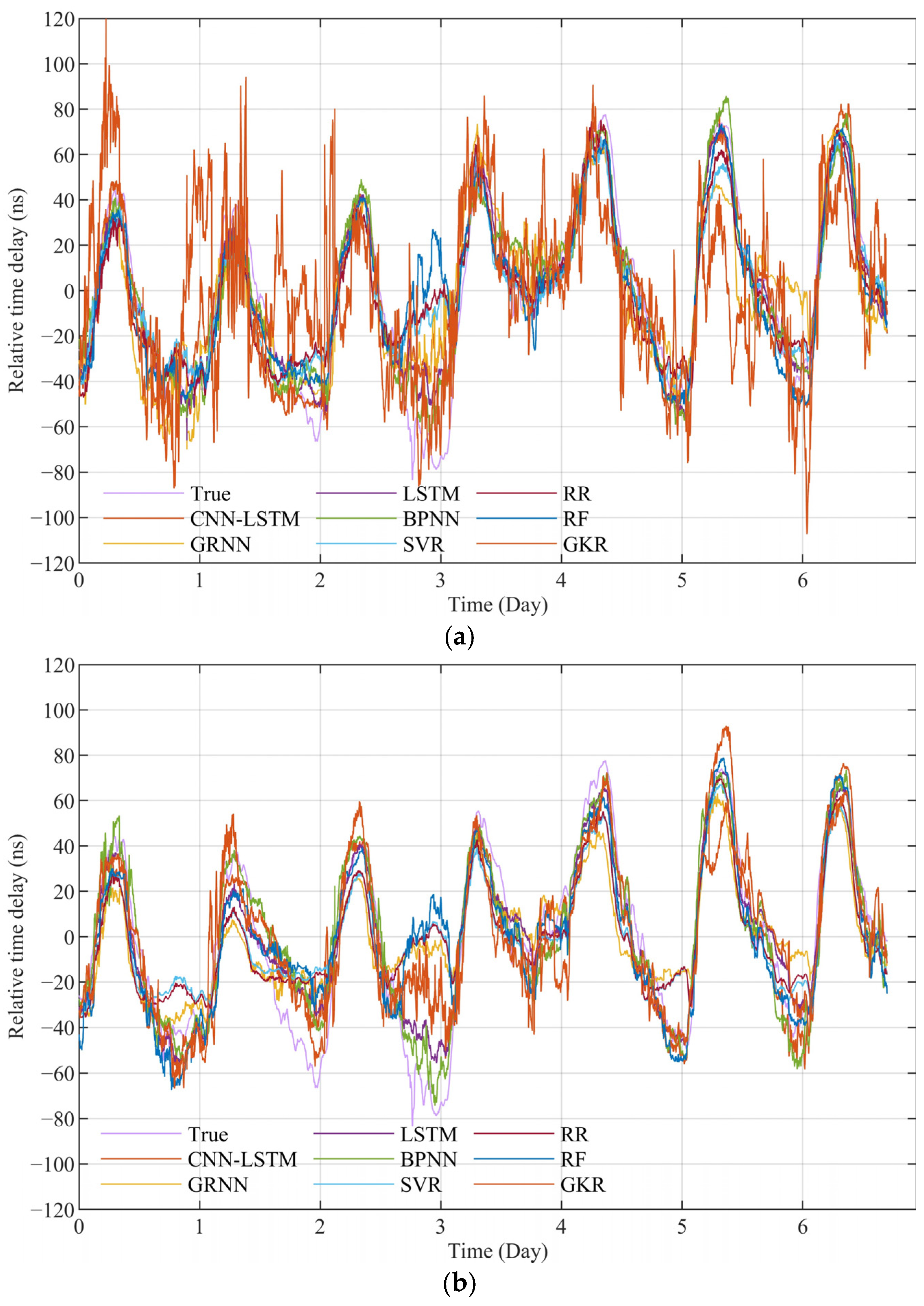
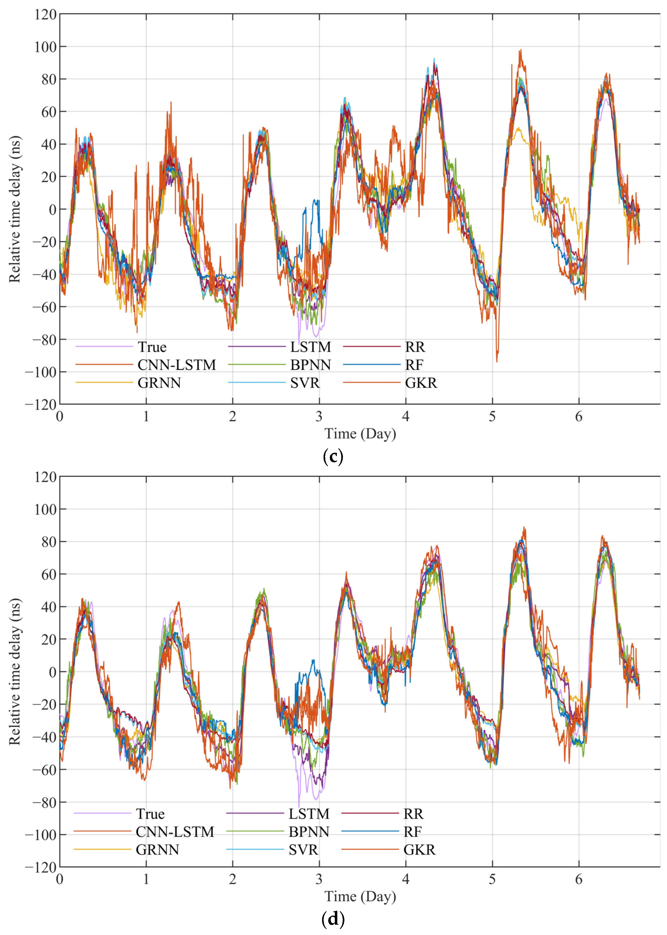
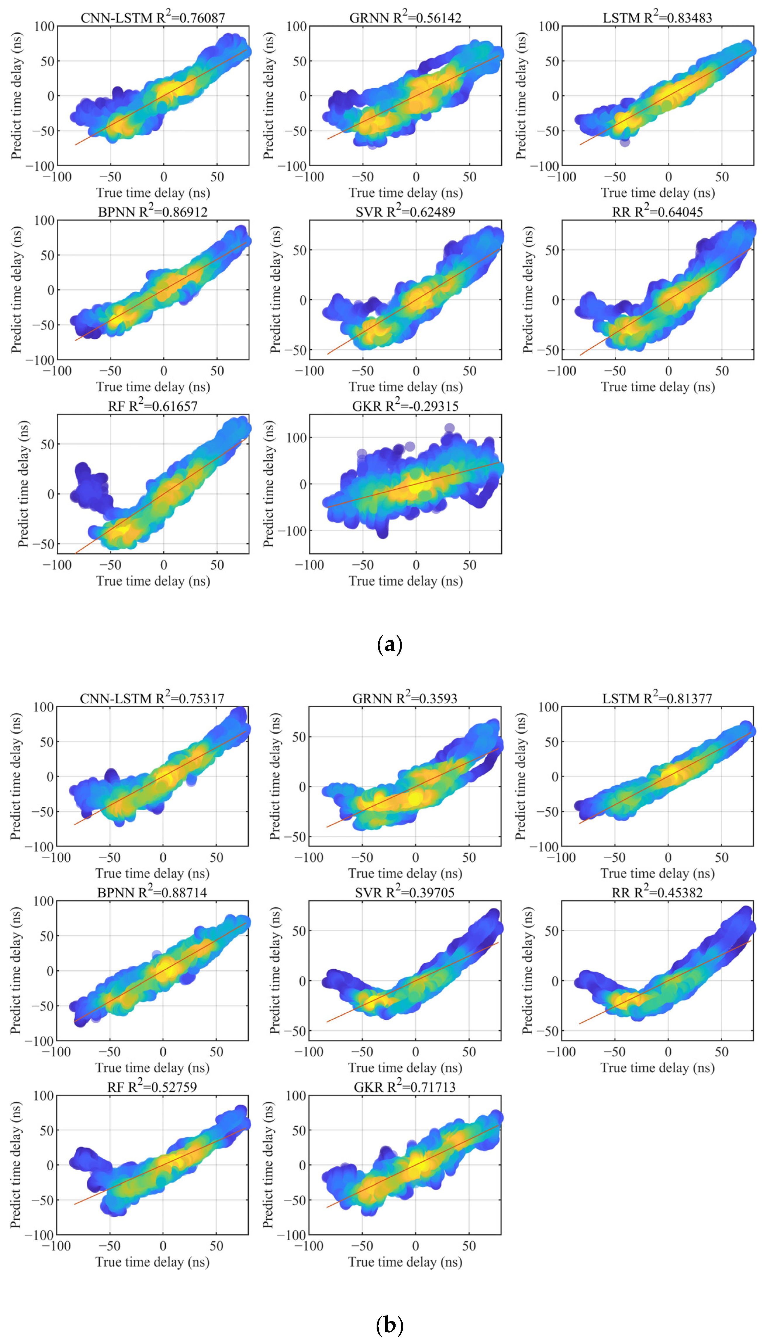
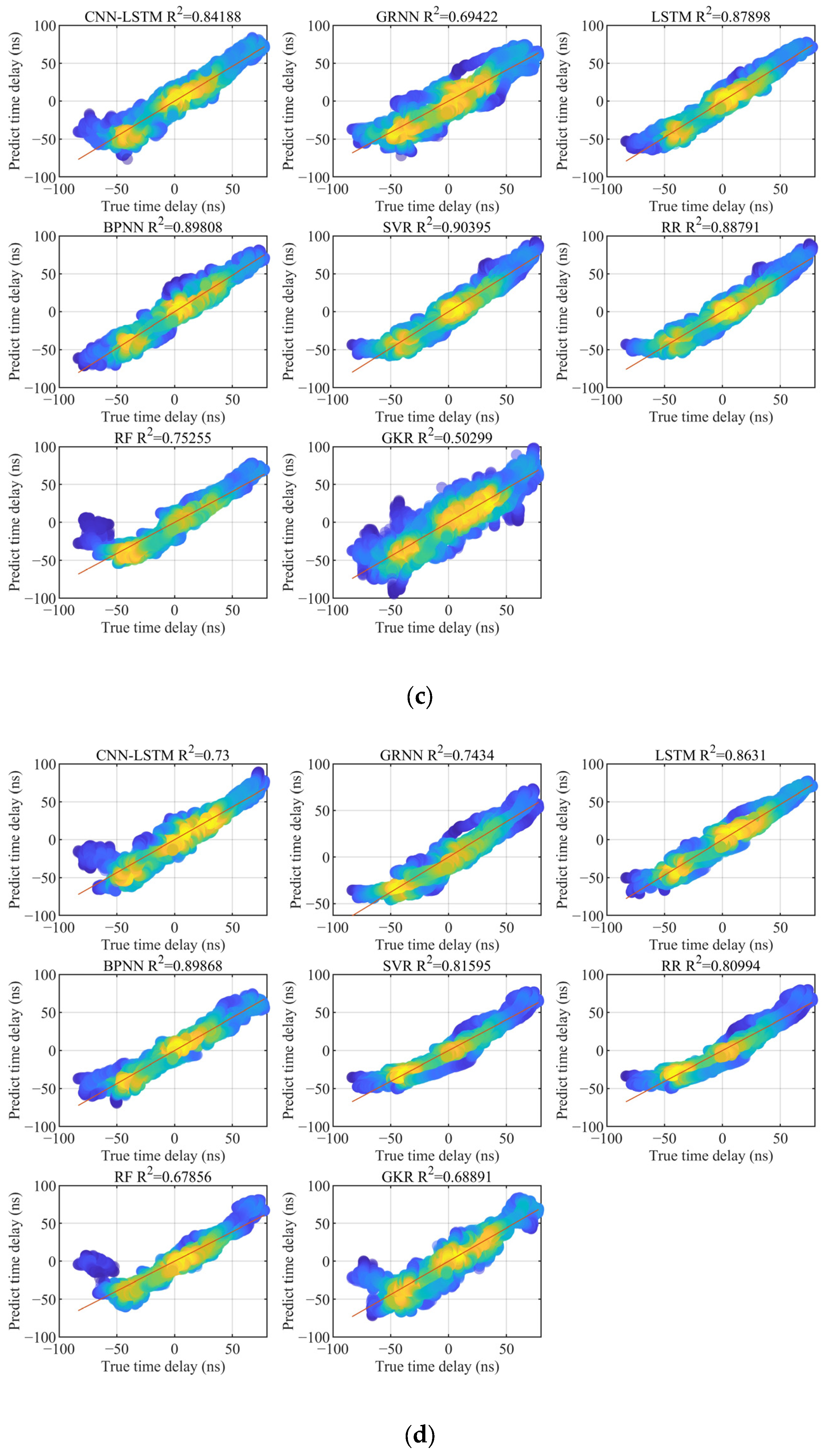
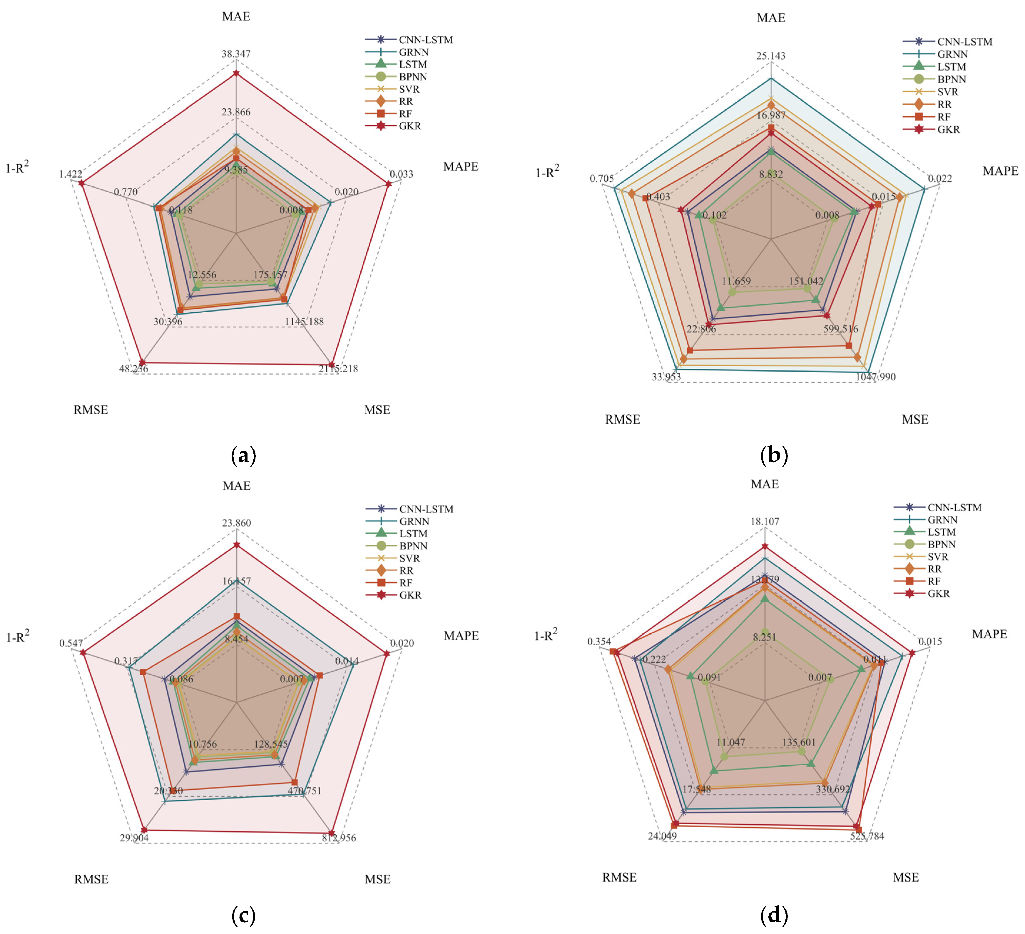
	PZWT-CNN-LSTM	13.999	1.192%	401.496	20.037	0.730	199.842

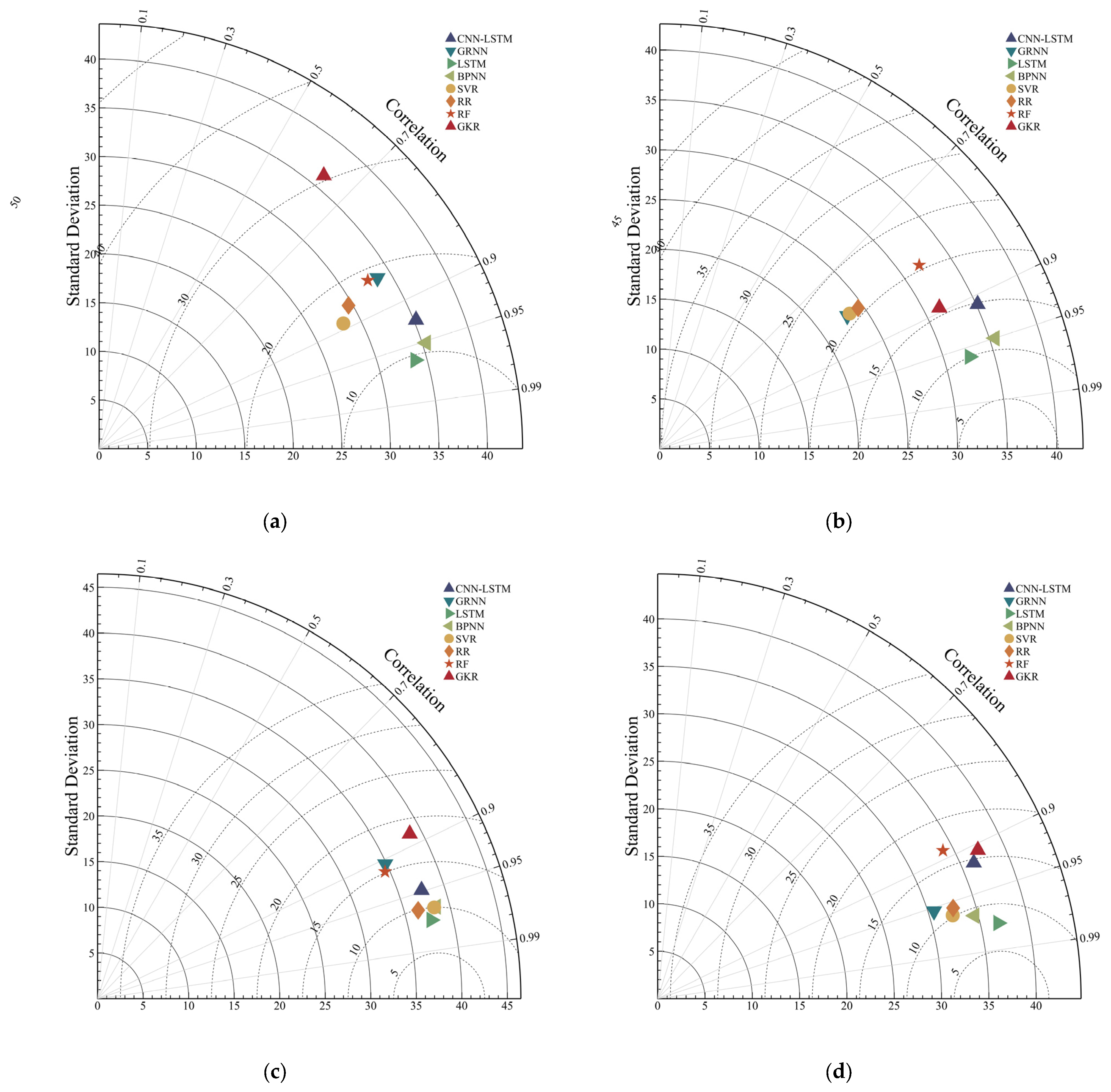
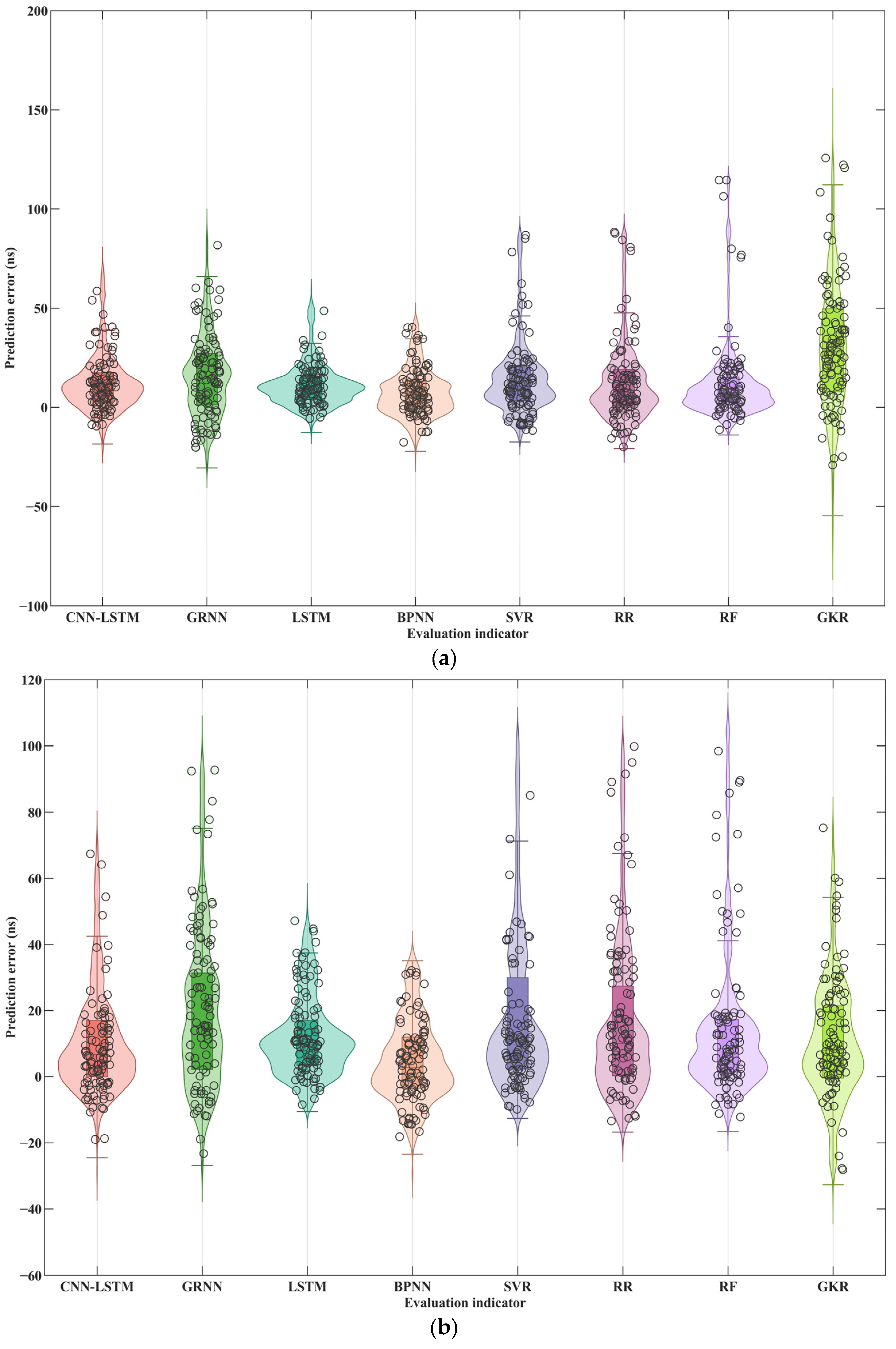
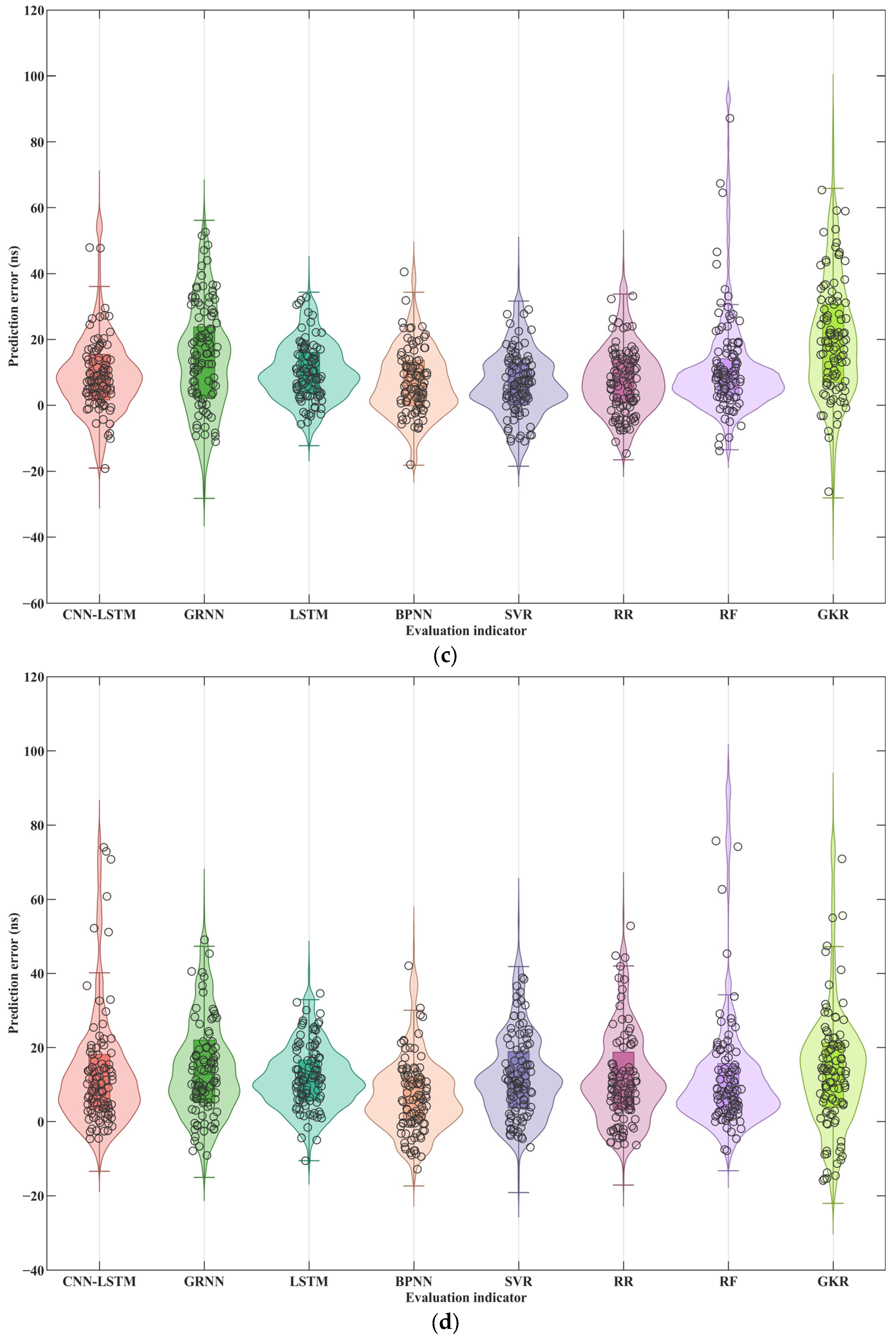
. In order to more intuitively reflect the comparison effect of data prediction, we draw the data curve diagram of the propagation delay prediction result of the Zhengzhou differential reference station, the $R^2$ diagram of the propagation delay prediction result data of the Zhengzhou differential reference station, the radar diagram of the propagation delay prediction result data of the Zhengzhou differential reference station, and the Taylor diagram of the propagation delay prediction result data of the Zhengzhou differential reference station. A violin plot of the station propagation delay prediction result data of the Zhengzhou differential reference station is shown in Figure 7, Figure 8, Figure 9, Figure 10 and Figure 11.

The multi-dimensional evaluation indicators of 32 models in the above table clearly show the influence of different input data and modeling methods on the prediction accuracy of eLoran propagation delay data of the target station. Comparing the same model of task 1 and task 2, the MAE of BPNN is reduced from 10.427 ns to 9.813 ns. RMSE decreased from 13.951 ns to 12.955 ns, $R^2$ increased from 0.869 to 0.887; Comparing the same model of task 3 and task 4, the MAE of the GKR method is reduced from 21.691 ns to 16.461 ns, the RMSE is reduced from 27.185 ns to 21.508 ns, and the $R^2$ is increased from 0.503 to 0.689. This shows that the path-based weighted processing of meteorological data integrates the spatial cumulative effect of meteorological factors on the path, corrects the one-sidedness of using the received weather station data for prediction, and shows that the path-based weighted meteorological data can improve the prediction accuracy of the propagation delay data of the target station.

Comparing the same model of task 1 and task 3, the MAE of RR decreased from 15.279 ns to 10.103 ns, the RMSE decreased from 23.123 ns to 12.910 ns, and the $R^2$ increased from 0.640 to 0.888. Comparing the same model of task 2 and task 4, the MAE of the RF method is reduced from 16.065 ns to 13.565 ns, the RMSE is reduced from 26.504 ns to 21.863 ns, and the $R^2$ is increased from 0.528 to 0.679. It shows that the delay data of the differential reference station on the path contains the meteorological information on the path, which can be used as an effective predictor to supplement the input data dimension and improve the prediction accuracy of the propagation delay of the target station.

Comparing various models in the four tasks, it is found that the BPNN model has the best comprehensive performance in the four tasks. Especially in task 4, the PZWT-BPNN model has an MAE of 9.168 ns, RMSE of 12.275 ns, $R^2$ of 0.899, and model training time of 15.576 s. Its performance is significantly better than that of linear models, traditional machine learning models, and other deep learning models and neural network models, which achieves a balance between prediction accuracy and prediction efficiency. It indicates that BPNN can achieve the best prediction performance under this specific task.

The curve of eLoran signal propagation delay prediction results of the Zhengzhou differential reference station intuitively shows the fitting degree between the prediction results of various prediction models and the true value under various prediction tasks. It is observed that the prediction curve of BPNN has the best fitting degree with the true value, especially in task 4. It can still accurately capture the change trend of propagation delay when the propagation delay fluctuates, and the prediction curve of the model without path weighting and differential reference station data on the path, such as PZNE-GKR, has a large deviation from the real value. The comparison shows that the prediction curve of task 2 and the task 2 model have a higher degree of fit than that of task 1, which verifies that the use of the path weighting method and differential reference station data on the path can improve the prediction accuracy of propagation delay. In addition, BPNN has no obvious over-fitting and under-fitting phenomenon, while LSTM, CNN-LSTM, and other models can capture part of the trend, but there are local prediction errors.

The closer the $R^2$ is to 1, the better the fitting effect of the model is. It is observed that the scatter distribution of BPNN is concentrated near the diagonal, especially when the $R^2$ of the PZNT-BPNN model is 0.904, which can be considered as a linear correlation. However, the scatter of the PZNE-GKR model deviated from the diagonal a lot, and its $R^2$ value was negative, indicating that the prediction of the model had little reference value. From the perspective of the input combination, the scatter of the model of task 2 was closer to the diagonal than that of task 1, and the scatter distribution of the model of task 3 was better than that of task 1. This intuitively proves that the use of the path weighting method and differential station propagation delay data on the path can enhance the prediction ability of the model. At the same time, in the same task, the $R^2$ scatter of BPNN is the most concentrated among all models, which again confirms the modeling advantage of BPNN in the task of predicting the propagation delay of the differential reference station on this path.

The radar map integrates MAE, MAPE, MSE, RMSE, 1-$R^2$ and other indicators. A smaller radar area indicates better comprehensive performance. In all tasks, the radar map of PZWT-BPNN shows the smallest area, which is better than other models in all indicators, while the radar map of the PZNE-RR model has a larger area. It shows that there are errors in multiple indicators. At the same time, the radar area of task 2 and task 3 is smaller than that of the corresponding model of task 1. For example, the radar map of the PZWE-GKR model has obvious shrinkage in MSE and RMSE indicators, and the MAE and MAPE indicators of the PZNT-SVR model are significantly better than those of the PZNE-SVR model. In addition, the radar map of BPNN has the smallest area among all the models for the same task, and each index is balanced.

Taylor plot evaluates the performance of the model by how well the correlation coefficient and standard deviation match the true value. The closer the correlation coefficient is to 1, and the closer the standard deviation is to the true value, the better the performance of the model. The correlation coefficient of the PZNE-GKR model is low, and the standard deviation is more deviated from the true value. The data of the task 2 and task 3 models are closer to the true value than the model in task 1. Among all modeling methods for the same task, the data points of the Taylor plot of the BPNN are always in the optimal region.

The violin plot shows the distribution density and range of prediction errors; the more concentrated the error is around 0 and the narrower the distribution range is, the better the stability of the model is. It is observed that the error distribution of the model in task 2 and task 3 is more concentrated than that of the model corresponding to task 1, and the error distribution of BPNN shows the characteristics of “narrow peak concentration”, indicating that its error is small and fluctuates stably. However, other models for the same task have relatively wide error distribution ranges, scattered peaks, and insufficient stability.

3.3. Summary

In this chapter, a multi-dimensional evaluation system covering MSE, MAE, MAPE, RMSE, $R^2$ and training time is constructed, which quantifies the prediction accuracy and computational efficiency of the model from multiple perspectives, and provides a scientific basis for the horizontal comparison of different models. In addition, by comparing the test results of 32 models of four kinds of prediction tasks, the key role of input data optimization is clarified. The use of the path weighting method and differential reference station propagation delay data on the path improves the performance of the model, that is, the prediction accuracy of eLoran signal propagation delay, which verifies the comprehensive optimal performance of BPNN in this prediction task.

4. Discussion

When the eLoran signal is propagated in long-distance scenes, the dynamic fluctuation of complex meteorological factors on the propagation path is an important factor restricting the improvement of the eLoran system timing accuracy. There is a complex nonlinear relationship between meteorological factors, and the traditional model is difficult to capture the complex nonlinear relationship due to its linear nature. Focusing on the key issue of meteorological factors in long-distance scenarios, this paper conducts research from four aspects: physical mechanism analysis, measured data optimization, prediction model construction, and model performance verification. A prediction model of eLoran signal propagation delay based on path-weighted meteorological data and propagation delay data of multiple differential reference stations is proposed, which provides a new idea for improving the timing accuracy in long-distance scenarios.

Firstly, through theoretical modeling and measured data analysis, this study reveals that the time delay data of the differential reference station on the path contains the meteorological information on the path, which can be used as an effective factor for the propagation delay prediction of the target differential reference station. This finding verifies the rationality of introducing differential reference station delay data into the prediction model, which is different from the traditional method that only relies on meteorological station data, and provides a new data source for improving the prediction accuracy. Meanwhile, through the measured data verification, it is found that the path weighting method can effectively improve the correlation between meteorological factors and eLoran signal propagation delay, and effectively correct the prediction error caused by using a single weather station’s data at the signal receiving site. This indicates that the path weighting method can make full use of the meteorological information along the propagation path, avoid the one-sidedness of single-point data, and lay a foundation for improving the model performance.

By designing four different comparison propagation delay prediction tasks, the modeling methods, such as the linear model and traditional machine learning model, as well as deep learning and neural network models, are systematically compared and verified on a unified high-quality data set. The experimental results show that, among the 32 models of the four tasks established, the BPNN model PZWT-BPNN using the weather data of the path weighting method and the propagation delay data of the differential reference station on the path performed best, with the MAE of the model prediction reaching 9.168 ns, RMSE 12.275 ns, and R² 0.899, while maintaining the efficient training speed of 15.576 s. This result fully demonstrates the superiority of the proposed PZWT-BPNN model in balancing prediction accuracy and computational efficiency. Compared with linear models, the model can better capture the complex nonlinear relationship between meteorological factors and propagation delay; compared with other traditional machine learning and deep learning models, it achieves higher prediction accuracy while ensuring training efficiency, which is more suitable for practical application scenarios of the eLoran system.

However, the research in this paper still has certain limitations, which need to be further improved in future research. In terms of data, the time span of data collection is short, which cannot cover the complete characteristics of four seasons; the sample size of extreme weather is insufficient, and the spatial resolution of data is insufficient, so it is difficult to completely and accurately describe the continuous dynamic changes in meteorological factors on the path. In addition, the study only involves a single transmission path from Pucheng to Zhengzhou and does not involve different scenarios, which may affect the generalization ability of the model. In terms of model design, the model does not explore the hybrid model or advanced ensemble learning model, fails to leverage the complementary advantages of different models, does not consider the priority of key meteorological factors in long-distance transmission scenarios, and the feature selection method is not clear. At the same time, the model does not consider the comprehensive influence of non-inherent factors such as electromagnetic interference, ground medium mutation, and spatial terrain change, which may limit the adaptability of the model in complex practical environments. In terms of engineering implementation, the current model is not designed for lightweight engineering practice. Although the training and reasoning efficiency can meet the experimental requirements, it is difficult to deploy in the resource-constrained receiver terminal, and the dynamic update mechanism is not built, so the model parameters cannot be adaptively adjusted according to new meteorological environmental data.

In view of the above shortcomings, corresponding improvement directions are proposed for future research, which are expected to further improve the research results and promote the practical application of the model. The specific future research directions are as follows: Firstly, collect a wider range of relevant data to make up for the deficiencies of current data; secondly, optimize the model structure and study new feature engineering methods to improve the model’s accuracy and adaptability; finally, promote the engineering implementation of the model to realize the application value of the research results in the actual eLoran system.

5. Conclusions

Focusing on the key problem that the dynamic fluctuation of meteorological factors in long-distance scenarios restricts the timing accuracy of eLoran system, and targeting the defect of traditional linear models being difficult regarding the understanding of the complex nonlinear relationship between meteorological factors and propagation delay, this paper conducts systematic research from four aspects: physical mechanism analysis, measured data optimization, prediction model construction and model performance verification. This study obtains the following core conclusions.

Firstly, the time delay data of the differential reference station on the eLoran signal propagation path contains the meteorological information of the path, which can be used as an effective factor for predicting the propagation delay of the target differential reference station; the path weighting method can effectively improve the correlation between meteorological factors and eLoran signal propagation delay, and correct the prediction error caused by using single-point weather station data at the receiving end.

Secondly, a prediction model of eLoran signal propagation delay (PZWT-BPNN model), based on path-weighted meteorological data and propagation delay data of multiple differential reference stations, is proposed. The experimental results show that among the 32 models established in four comparative tasks, the PZWT-BPNN model has the best performance, with the prediction MAE of 9.168 ns, RMSE of 12.275 ns, R² of 0.899, and training speed of 15.576 s, achieving a good balance between prediction accuracy and computational efficiency.

Third, the proposed model and research method provide a new idea for improving the timing accuracy of the eLoran system in long-distance scenarios, and lay a theoretical and experimental foundation for the subsequent optimization and engineering application of the propagation delay prediction model.

Finally, this study also clarifies the limitations in data, model design and engineering implementation, and puts forward clear future research directions, which are of great significance for further improving the research results and promoting the practical application of the model in the eLoran system.