Uncoupled CFD-FEA Methods for the Thermo-Structural Analysis of Turbochargers ^†

Abstract

In turbocharger design, the accurate determination of thermally induced stresses is of particular importance for life cycle predictions. An accurate, transient, thermal finite element analysis (FEA) of turbocharger components requires transient conjugate heat transfer (CHT) analysis. However, due to the vastly different timescales of the heat transfer mechanisms in fluid and in solid states, unsteady CHT simulations are burdened by high computational costs. Hence, for design iterations, uncoupled CFD and FEA approaches are needed. The quality of the uncoupled thermal analysis depends on the local heat transfer coefficients (HTC) and reference fluid temperatures. In this paper, multiple CFD-FEA methods known from literature are implemented in a numerical model of a turbocharger. In order to describe the heat transfer and thermal boundary layer of the fluid, different definitions of heat transfer coefficients and reference fluid temperatures are investigated with regard to calculation time and accuracy. For the transient simulation of a long heating process, the combination of the CFD-FEA methods with the interpolation FEA approach is examined. Additionally, a structural-mechanical analysis is conducted. The results of the developed methods are evaluated against experimental data and the results of the extensive unsteady CHT numerical method.

1. Introduction

The growing competition, challenging requirements for an efficiency, and rigorous restrictions on exhaust emissions in a transportation sector are forcing the companies involved to deploy time and cost improved design procedures to increase the quality of individual vehicle components. The further development of turbochargers, which significantly enhance the performance of the whole engine, perfectly conforms with the leading trends in automotive industry.

In pursuit of improved engine performance, exhaust gas temperatures are being continuously increased. However, a high temperature of a flow at the inlet to the turbine, together with the transient operating conditions, unavoidably leads to high thermal stresses in the turbine housing and turbine wheel [1]. Thus, in order to account for the thermal stresses as part of the standard design process, fast calculation methods are required to determine transient temperature fields in a turbocharger.

Several methods to conduct thermo-structural analysis of a turbocharger are reported in literature. However, most of the published research focuses on the turbine housing. Heuer et al. [2] applied 3D transient conjugate heat transfer (CHT) simulations to twin-entry turbine housing with an integrated manifold designed for an application within trucks. The research revealed the locations of highest stress in the turbine housing, which occur during transient operation. Ahdad et al. [3] developed a FE model of a turbine housing for the complex duty cycle. The semi-empirical approach utilizes empirical correlations to describe the thermal boundary conditions applied to the model. Other thermo-structural investigations of turbine housing are presented by Oberste-Brandenburg et al. [4] and Guo et al. [5].

In contrast to the turbine housing, the turbine wheel has only rarely been a subject of thermo-mechanical research. Heuer et al. [6] extended his research to the turbine wheel of a turbocharger. The investigation enabled an identification of the critical zones on a turbine wheel—where the stresses reached the highest values. Moreover, it was proven that the thermal stresses play an important role in the development of stress peaks in the fillets on the back of the turbine wheel and on the blade roots. Similar results were reported by Makarenko et al. [7]. Diefenthal et al. [8,9,10] increased the accuracy of the simulation approach of Heuer et al. [6]. Their numerical calculations were validated by transient experimental data. Furthermore, the 3D thermo-structural analysis has proven that one-dimensional approaches are not sufficient to capture the transient temperature fields with regard to thermo-mechanical fatigue. Hence, three-dimensional or empirical methods have to be used.

Furthermore, most of the above research is based on CHT methods. These approaches are firstly, burdened by high computing times, and secondly, have low potential for an automatisation of the design process. The high requirements for mesh resolution frequently involve creating conforming interfaces between fluid and solid domains. This implies a high user effort in investigations of multiple fully-modeled geometries. Against this background, the main objective of the present work was the development of fast CFD-finite element analysis (FEA) simulation methods in order to model transient solid/fluid heat transfer in turbine wheel and turbine housing of a turbocharger. Depending on their accuracy, these CFD-FEA calculation schemes can be applied both in automatized, early stage investigations of various turbine designs and in high quality evaluations of the final turbocharger designs tested under time-dependent operating conditions. Hence, in following analysis, four different CFD-FEA approaches, as described in literature, are further investigated. This paper creates also a link between setup of individual numerical methods, their theoretical background, and the results. The methods were validated against test data and against the results of the extended CHT numerical method described in Diefenthal et al. [8].

2. Thermal Shock Test

In the operation of a turbocharger, the highest thermal stress of the turbine components occurs during transient heating processes. Typical engine operation conditions result in abrupt changes to exhaust gas temperatures of several hundred Kelvin [9]. Therefore, it is assumed that the maximum thermal stress in the real driving cycle arises when the turbine inlet temperature is changed abruptly. Hence, in this work, a simplified, equivalent process called thermal shockwais used for the purpose of thermo-mechanical analysis.

In the thermal shock procedure the fluid inlet temperature to a turbocharger is rapidly changed in a step function at time point $t_0$ from $T_{FL,-\infty }$ to $T_{FL,\infty }$, as graphically depicted in Figure 1. The resulting time-dependent, logarithmic growth of solid body temperatures during thermal shock is situated between the cold turbine state at operating point 1 (OP1) and the hot turbine state at operating point 2 (OP2).

The thermal shock procedure was applied to a commercial vehicle turbocharger with a scalloped turbine wheel of approximately 90 mm diameter. For this purpose, a test rig which was able to impose both rapid changes in turbine inlet temperatures and monitor the transient temperatures on the turbine wheel (TW) and turbine housing (TH) was designed. The temperatures measured are accurate to within +/− $3.2$ $\mathrm{K}$ at 600 ${}^{\circ }\mathrm{C}$. The positions of four and six K-Type thermocouples on TW and TH respectively, are presented in Figure 1. A detailed description of the test rig and measurement setup is given in Tadesse et al. [11].

3. Calculation Methods and Methodology

Generally, two main calculation approaches to transient fluid/solid heat transfer are described in literature: conjugate heat transfer (CHT) (or fully coupled) methods and uncoupled (or loosely coupled) CFD-FEA methods.

In CHT approaches, a direct coupling of the fluid and solid body using the same discretization and numerical principle for both zones is used. The fluid equations and solid heat conduction equation are solved simultaneously in one solver. Furthermore, continuity of the temperatures and the heat fluxes at the fluid/solid interfaces is ensured by solving the energy equation at the coupled boundaries, which results in a high accuracy of the numerical simulation. The examples of the CHT approach are presented in Han et al. [12], Rigby and Lepicovsky [13], and Bohn et al. [14]. The CHT methods, however, are mainly confined to steady state simulations. An unsteady CHT calculation demands very high computing capacities, since the timescales of convective and conductive heat transfer differ by a factor of about ${10}^4$ [15]. However, there are some transient applications of CHT methods presented in Okita [16], Okita and Oldfield [15], and Diefenthal et al. [9,10].

A possible solution to the problem of different timescales in the conduction and convection processes is a separate calculation of fluid and solid states by two independent solvers. Hence, in contrast to CHT methods, different fluid and solid codes can be flexibly used. The uncoupled CFD-FEA approaches are primarily based on the four main iteration schemes between CFD and FEA solvers: flux forward temperature back (FFTB) [17,18], temperature forward flux back (TFFB) [19], heat transfer coefficient forward temperature back (hFTB) [17,20], and heat transfer coefficient forward flux back (hFFB) [21] methods. The hFTB scheme deserves special attention, since—in this particular calculation scheme—the number of iterations between CFD and FEA solvers, which are required for satisfying the accuracy of the results, may be significantly reduced. The typical hFTB approach uses the convective heat transfer equation (Equation (1)) to generate the thermal boundary conditions (heat transfer coefficient h and reference fluid temperature $T_{FL,ref}$) for a subsequent FEA calculation:

$$h=q_w/(T_w-T_{FL,ref}).$$

(1)

During the iteration process, the resulting wall temperature is returned from the FEA solver to the CFD simulation, which gives the hFTB method its name. The main drawback of the uncoupled CFD-FEA procedure is the iterative invocation of the CFD solver, which inevitably increases the computing time. Hence, fast calculation methods have to reduce the number of necessary iterations to a minimum. In each iteration, the locally determined wall temperature values $T_w$ approach those of the converged solution. Interestingly, under the assumption of a linear relationship between convective heat flux across the boundary layer and the driving temperature difference, the heat transfer coefficient (HTC) in the ideal case is properly described by the ratio of $q_w$ to $(T_w-T_{FL,ref})$, and hence, independent of the thermal boundary conditions (or independent of the different values of $T_w$). On the contrary, the reference fluid temperature $T_{FL,ref}$ strongly depends on those thermal boundary conditions. Therefore, the accuracy of the entire loosely coupled CFD-FEA calculation relies on the formulation of $T_{FL,ref}$. According to the literature, the definition of the reference fluid temperature should capture the local changes in the thickness of the thermal boundary layer. For the simplified case of laminar flow, Schlichting [22] suggests defining the displacement thickness of a fluid thermal boundary layer at about 99% of its respective freestream value. In this context, a brief analysis of boundary layer simulation methodology is presented.

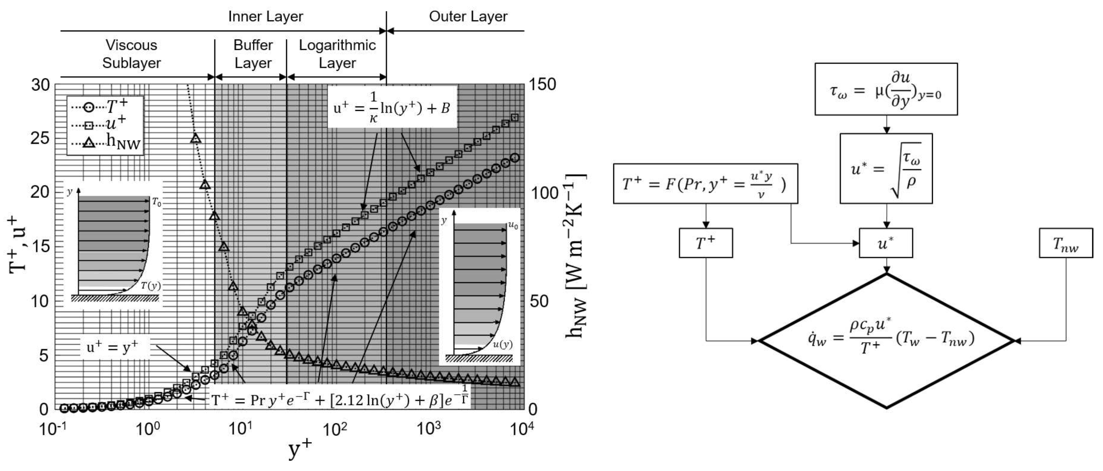
Based on the analysis of Tennekes and Lumley [23], the flow near the wall is divided into three layers, as given in Figure 2—the inner layer, the logarithmic layer, and the outer layer. The dimensionless velocity profile $u^{+}$ in the first two layers, which are of particular importance for numerical modeling, are described by:

$$u^{+}=y^{+}for0<y^{+}<5;u^{+}=\frac{1}{\kappa }ln\left(y^{+}\right)-Bfor30<y^{+}<350;$$

(2)

where for kinematic viscosity $\nu$, vertical distance to the wall y, wall shear stress ${\tau }_{\omega }$, and density $\rho$, the dimensionless wall distance $y^{+}$ together with friction velocity $u^{*}$ are defined as:

$$y^{+}=\frac{u^{*}y}{\nu }for{u}^{*}=\sqrt{\frac{{\tau }_{\omega }}{\rho }}.$$

(3)

Similarly, the non-dimensional temperature profile is described by [24]

$$T^{+}(y^{+},Pr)=Pr{y}^{+}{e}^{-\mathsf{\Gamma }}+[2.12ln\left(y^{+}\right)+\beta ]e^{-1/\mathsf{\Gamma }}forPr=\frac{\mu C_p}{\lambda },$$

(4)

where $Pr$ is the Prandtl number, $\beta \left(Pr\right)$ and $\mathsf{\Gamma }(Pr,y^{+})$ are the coefficients, $\mu$ is the dynamic viscosity, $C_p$ the heat capacity, and $\lambda$ the thermal conductivity of the fluid. Finally, based on the above considerations, the heat flux through the wall $q_w$ is defined. Due to the benefits regarding the stability of the numerical scheme, in several commercial flow solvers, the following formulation of heat flux $q_w$ is proposed:

$$q_w=\frac{\rho C_p{u}^{*}}{T^{+}(y^{+},Pr)}(T_w-T_{nw})=h_{nw}(T_w-T_{nw})for{h}_{nw}=\frac{\rho C_p{u}^{*}}{T^{+}(y^{+},Pr)},$$

(5)

In Equation (5), the value of $q_w$ is calculated based on the near-wall heat transfer coefficient $h_{nw}$ and corresponding fluid reference temperature $T_{nw}$. In addition, $h_{nw}$ depends on the value of $T^{+}$ at the first element nodes next to the wall. The profiles of $T^{+}$, $y^{+}$, and $h_{nw}$ over $y^{+}$, which are calculated for regular operating conditions of the investigated turbocharger, are presented in Figure 2. The similarity between the temperature and velocity profiles results from a Prandtl-number close to unity (valid for gases), and corresponds with the Reynolds analogy. Moreover, the small difference $T_w-T_{nw}$ leads to high values of $h_{nw}$ at the first nodal element from the wall. The plot of $h_{nw}$ logarithmically declines for increasing values of $y^{+}$. Thus, between $y^{+}=1$ and the logarithmic layer, $h_{nw}$ decreases by 93.4%, compared to its value at $y^{+}=1$, while the changes within the logarithmic layer remain under 2.2%.

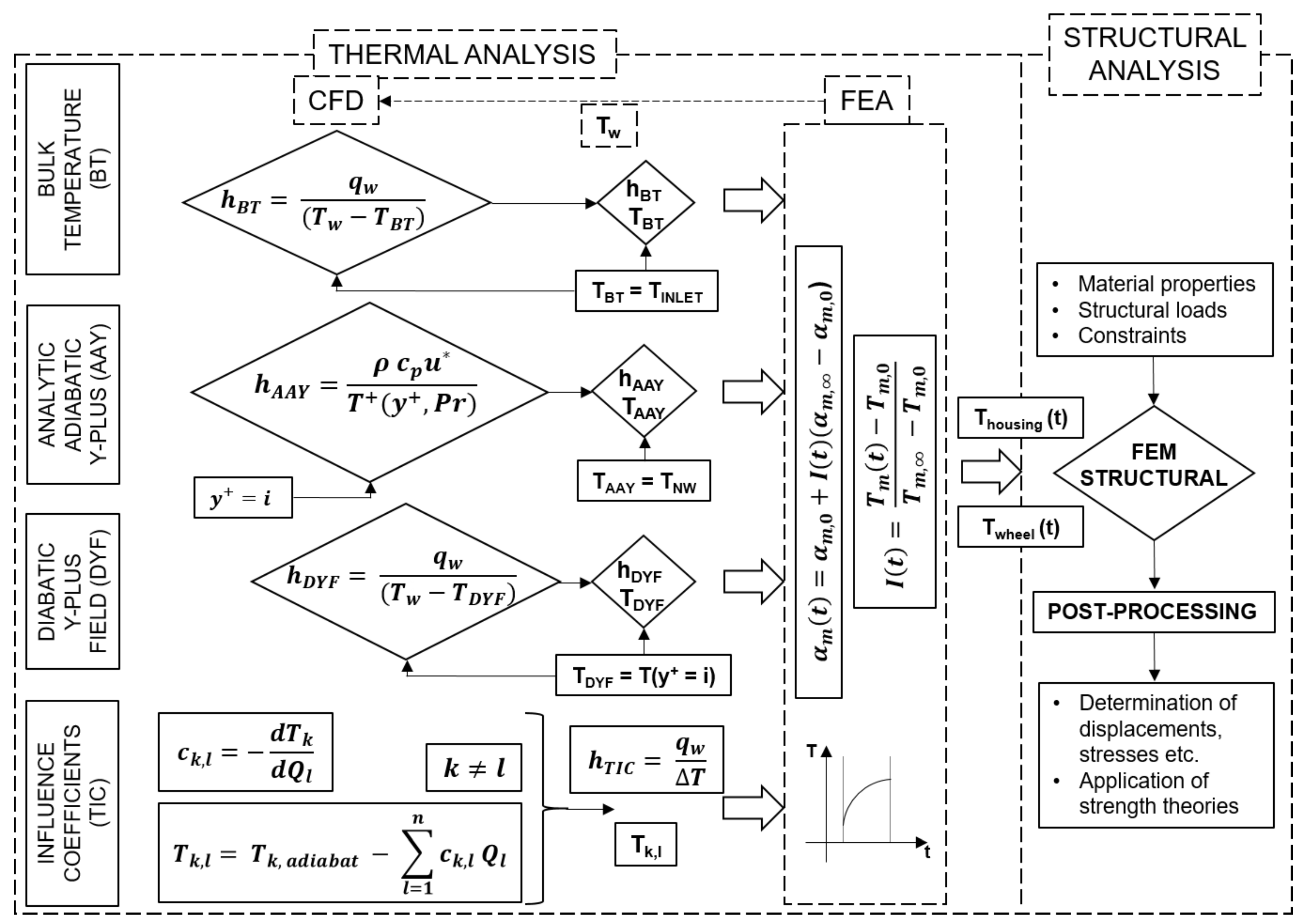
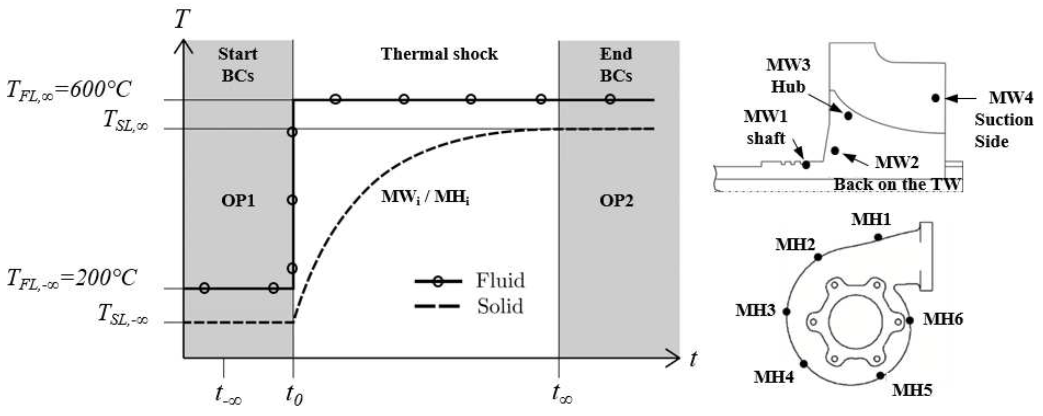
In this paper, the main CFD-FEA methods found in the literature are investigated with regard to thermo-structural analysis: the simple bulk temperature (BT) method, the analytic adiabatic Y-plus (AAY) method [25], the diabatic Y-plus field (DYF) method [26], and the temperature influence coefficient (TIC) method [27,28]. These approaches were applied to the numerical model of the turbocharger in order to calculate the heat transfer and temperature distribution in the volute and turbine wheel at operating points OP1 and OP2 (cf. Figure 1). Additionally, the set-up of these methods was investigated to identify the simulation settings, which led to the highest quality of results. For the thermal shock calculations, all four approaches were integrated with the TFEA-EXPO interpolation method [9]. In the subsequent step, structural analysis of the volute and turbine wheel was conducted, as presented in Figure 3.

In the BT approach, an arbitrarily chosen, constant bulk temperature $T_{BT}$ is used as the fluid reference temperature. In the investigated case, $T_{BT}$ is set equal to the fluid temperature at the inlet of the turbocharger. However, the definition of $T_{ref}$ in the BT method leads to inaccuracies in the description of local heat transfer through the thermal boundary layer. Hence, in order to achieve higher accuracy in this approach, additional hFTB iteration loops are required. The thermal boundary conditions for diabatic CFD simulations are estimated to be about 90%–99% of the inlet air temperature.

The AAY method utilizes a simple adiabatic CFD calculation and employs the previously discussed analytical definition of the HTC from dimensionless boundary layer equations. Corresponding to the plot of $h_{nw}$ in Figure 2, the heat transfer coefficients do not significantly change for higher values of $y^{+}$. Hence, in the AAY approach, the heat transfer coefficients are determined using a non-dimensional temperature $T^{+}(y^{+},Pr)$ evaluated further away from the viscous sub-layer region at $y^{+}$-values of 5, 60, and 250, in order to reduce the deviations of $h_{AAY}$ in the case of inaccurate thermal boundary conditions. The near-wall temperature $T_{nw}$ is used as a fluid reference temperature, due to the assumption that in adiabatic simulations the difference between the $T_{nw}$ and fluid temperatures at the edge of thermal boundary layer is negligible [25]. Therefore, hFTB iterations for the AAY method are not useful.

In the DYF approach, the HTC is defined based on Equation (1). The $T_{FL,ref}$ are obtained based on the local fluid temperatures on the surface at fixed dimensionless distances of $y^{+}=5$, 60, and 250 to the diabatic wall. This procedure also exploits the aforementioned similarity between velocity and temperature profiles in turbochargers in order to describe the thickness of the thermal boundary layer [26]. Analogous to the BT method, the wall temperatures for CFD calculations were estimated to be about 90% to 99% of the inlet air temperature. Furthermore, additional hFTB iterations loops are possible.

The TIC approach was originally developed for investigations of windage and heat transfer in rotor-stator cavities [27,28]. In this method, the relevant surfaces for heat transfer are divided into k zones. For determination of the heat transfer coefficients and reference fluid temperatures, several adiabatic and diabatic CFD simulations are conducted. The main objective of the method is to capture the interaction in heat transfer between individual surfaces by means of influence coefficients $c_{k,l}$. Subsequently, the values of $c_{k,l}$ are utilized to obtain the reference fluid temperatures. The exact description of the TIC method is given by [27,28].

All four CFD-FEA approaches provide the subsequent TFEA-EXPO method with necessary start and end boundary conditions. This interpolation approach assumes a linear change of HTCs over the wall temperatures for every cell m of the housing and turbine wheel. Due to the exponential behavior of the wall temperatures, the TFEA-EXPO approach results in an exponential behavior of HTCs over time. More information on the TFEA-EXPO method can be found in Diefenthal et al. [9]. In the final step of analysis, the transient temperature fields are exported to a structural FEM model, as presented in Figure 3.

4. Thermal Analysis

In this section the combined, uncoupled CFD-FEA/TFEA-EXPO approaches are compared with experimental data and a reference coupled approach—known as the frozen flow (FF) method. Due to the different timescales in fluid and solid states, the FF method assumes the pressure and velocity distributions to be constant over certain time periods. Hence, the equations of mass, momentum, and turbulence are not solved, and consequently, larger time steps can be applied. The numerical model of the investigated turbocharger was simulated in Ansys CFX and comprises the turbine housing, turbine wheel and inlet and outlet pipes. As presented in Figure 4, the bearing housing and the compressor were not considered in the model. Under the assumption of circumferential periodicity in turbine wheel, a single rotor passage was simulated by using a mixing plane at the rotor/stator interfaces. The defined thermal boundary conditions at the outer surfaces of the shaft, which describe the heat fluxes to the gas cavity ($h_1+T_{ref,1}$), to the lubricant oil ($h_2+T_{ref,2}$) and to the compressor side (q), were based on the experimental data. Moreover, assuming that the radiative heat fluxes to the bearing housing are small, the heat shield at the back of the turbine wheel was set as adiabatic. The mesh of the whole turbine model was discretized by approximately 3.7 million nodes in the fluid state and 2.5 million nodes in the solid body. In the fluid boundary layer, $y^{+}$ was lower than one. A mesh study proved the independence of the results regarding spatial resolution. The low-Reynolds $k\omega -SST$ turbulence model was applied. Variable time steps were used during the calculation, as detailed above. A more detailed description of the FF method is given in [8].

The comparison of the individual CFD-FEA approaches at stationary OP1 and OP2 without further hFTB iterations is presented in Figure 5. Fundamentally, the considered methods achieve higher accuracy in the turbine housing than in the turbine wheel. Furthermore, more intense heat transfer through the fluid/solid boundaries in OP2 negatively influences the accuracy of the results. However, in both OPs, very good agreement with experimental data is obtained by means of the AAY and DYF approaches. These methods are further investigated with regard to the value of $y^{+}$. In the case of AAY simulations, the highest accuracy was observed for simulations with $y^{+}$ equal to 250–0.54% and 2.44% of averaged relative error over MH1-MH6/OP1 and MW1-MW4/OP1 respectively, and 1.31% and 4.88% of averaged relative error over MH1-MH6/OP2 and MW1-MW4/OP2 respectively. These results correspond with the values reported by Karamavruc et al. (2016). Analogously, in the case of the DYF approach, the overall highest accuracy in OP1 and OP2 was also achieved in simulations where $y^{+}$ was set to 250. However, slightly smaller relative errors were identified for $y^{+}$ equal to 60, especially at measuring points at TW. This is mainly attributable to a locally thinner boundary layer at TW than at TH for diabatic calculations. For $y^{+}=250$ the resulting temperature distributions inside the turbine wheel are displayed as a cross-section in Figure 6. For reference the Frozen Flow results are displayed in the middle with OP1 on the left and OP2 on the right. It can be seen that the deviations of the AAY method generally trend towards increased temperatures. Examples for this are the increased temperature at the back of the turbine wheel in OP1 and the increased temperatures at inlet and turbine wheel back in OP2. Conversely, the DYF slightly underestimates the resulting temperatures. This can be seen at the leading edges in OP1 and OP2, and a section towards the trailing edge on both operating points.

The two other approaches—BT and TIC—lead to higher deviations at individual measuring positions. For the BT approach, the main drawback of the method remains the previously mentioned lack of physical correlation between fluid reference temperature and local heat transfer. In contrast, the TIC method provides very promising results. However, this approach requires experience of the user in order to identify the walls characterized by similar heat transfer conditions a priori, and to define the individual surfaces with respective temperature influence coefficients accordingly.

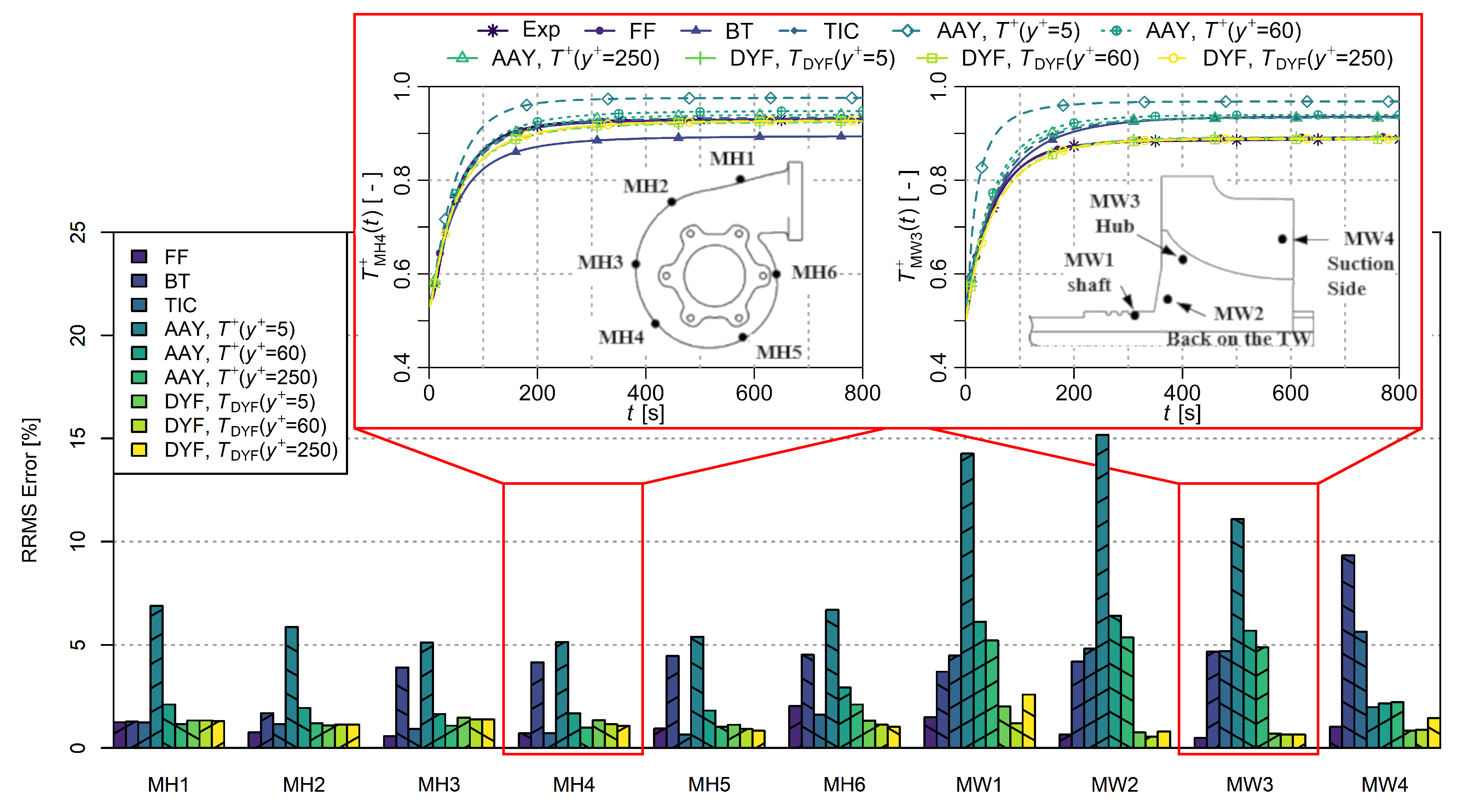
The accuracy of the individual approaches in OP1 and OP2 is reflected in transient temperature plots, which are obtained by the TFEA-EXPO method. In particular, the deviations in OP2 prove a noticeable influence on values of relative root mean square (RRMS) error. In Figure 7, the plots of temperature for the considered CFD-FEA methods and the (computationally expensive) reference CHT method—the FF approach—are compared with experimental data. The values of RRMS errors at all measuring positions for the first 800 $\mathrm{s}$ of the thermal shock procedure are depicted in Figure 7. As expected, the highest accuracy in TH and TW was achieved by the DYF approach—under 3% of RRMS error. That was followed by the AAY method, although this simulation approach resulted in relatively higher RRMS values at TW—under 7% for calculations with $y^{+}$ equal to 60 and 250. As in the case of OP1 and OP2, and consistent with theory, the AAY approach provided significantly better agreement with experimental data for higher values of $y^{+}$. Moreover, the previous comments on the accuracy of the BT and TIC methods remain valid. However, it must be emphasized that, in case of the TIC approach, the additional division of walls to smaller surfaces would increase the quality of the results. The methods achieved reductions in calculation time in reference to the FF method by factors of: $0.77$ (BT), $0.52$ (AAY), $0.74$ (DYF), and $0.94$ (TIC), as shown in

Table 1. Computational Time required for the various methods.

Method	FF	AAY	DYF	TIC	BT
Stationary CHT [h]	60 + 60	-	-	-	-
Stationary CFD (adiabatic) [h]	-	70+70	-	70 + 70	-
Stationary CFD (diabatic) [h]	-	-	144 + 144	192 + 96	144 + 144
Stationary FEA [h]	-	25 + 25	25 + 25	25 + 25	36 + 36
Stationary CFD (cold) [h]	-	130	130	130	130
Transient Temperature	572	40	40	40	40
Total [h]	692	360	508	648	530
Total [%]	100	52	73.4	93.6	76.6

. A short calculation time of AAY method is explained by a fast convergence of adiabatic CFD simulations, which are required for a determination of thermal boundary conditions at subsequent FEA simulations. Conversely, the TIC method requires several CFD simulations, which is reflected in the computational effort.

5. Structural Analysis

Structural-mechanical models of the turbine wheel and turbine housing were developed to conduct thermo-mechanical analysis. The main objective of this investigation was to compare different CFD-FEA calculation methods with regard to the total stress.

Accounting for slow solid temperature changes in the heating process, a steady-state model was utilized for the structural-mechanical calculations. The same mesh was used as in the thermal CFD-FEA simulations. Based on Heuer et al. [6], Ibaraki et al. [29], and Ohri and Shoghi [30], the deformations in the turbine wheel were considered to be isotropic and linear elastic. In contrast, the FEM model of the turbine housing accounted for plastic deformations [31] and stiffening of the material. The thermal expansion coefficient, the Young’s modulus, and the density changed as part of a function of temperature. The thermal and mechanical loads (due to the rotational speed) were applied to the structural FEM model. The pressure and gravitational forces were neglected.

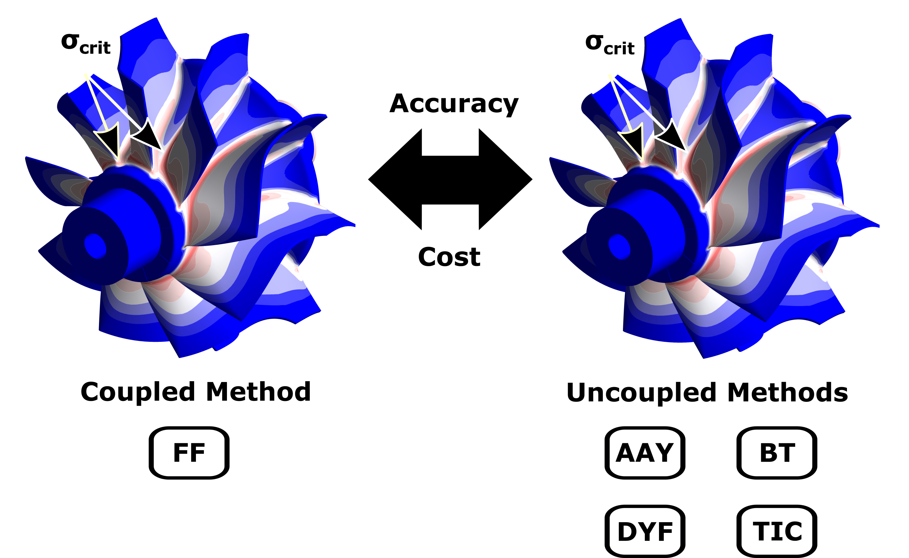
In order to compare the accuracy of individual CFD-FEM methods with regard to structural analysis, the transient plots of the von Mises stress at chosen critical zones on turbine wheel ZW (Zone Wheel) and turbine housing ZH (Zone Housing) are presented in Figure 8. The locations of zones were originally determined based on the transient temperature fields obtained using the FF method, and they correspond with the results reported by Diefenthal et al. [10], Heuer et al. [6], and Ibaraki et al. [29]. The high values of stress at both zones are caused by locally varying fluid/solid heat transfer and the resulting inhomogeneous temperature distribution. Interestingly, ZW all approaches led to satisfying results, with the highest deviation of the maximum von Mises stress equal to 4.59% for DYF method (in reference to structural analysis based on the temperature fields determined by FF-method). When considering ZH, the highest accuracy was achieved by the TIC and AAY methods, with −4.91% and −5.22% deviations from the maximum von Mises stresses respectively. As expected, the AAY and DYF methods display better agreement with the reference calculation for higher values of $y^{+}$.

Thus, considering the results of the thermal and structural analysis, both AAY and DYF are suitable to calculate transient fields of temperature by means of only one CFD-FEA iteration. Therefore, these methods are an interesting choice for the thermo-structural investigations due to their good accuracy and short computational time. Furthermore, the quality of the results provided by the TIC approach depends on the user experience and setup of the method. In principle, the application of this method for thermo-structural analysis is possible. In contrast, although the BT method leads to satisfying results in the case of the considered values of stress, investigation of local heat transfer at different locations at TW and TH revealed higher calculation errors. Hence, this method is not recommended as a numerical tool for the calculation of fluid/solid heat transfer. To conclude, the choice of the optimal calculation method for the considered numerical problems is a matter of requirements for calculation times, user input and accuracy.

6. Conclusions

In this paper, four uncoupled CFD-FEA approaches are combined with the interpolation FEA method in order to calculate transient fluid/solid heat transfer in the turbine wheel and turbine housing during a thermal shock test. The main advantages of these simulation schemes is an computationally-efficient calculation method of long transient heat transfer processes and a high potential for process automatization. The presented methods differ from each other by the definition of the heat transfer coefficients h and fluid reference temperatures $T_{FL,ref}$.

The “classical” formulation of the heat transfer coefficients is based on the artificially introduced definition of bulk temperature. This bulk temperature method is unable to capture the local heat transfer through the thermal boundary layer, which results in lower accuracy of heat transfer predictions. In the case of the turbocharger, the averaged RRMS error of the BT method between the measured and simulated values of temperatures amounted to 3.33% in the turbine wheel, and to 5.48% in the turbine housing. On the contrary, the analytic adiabatic Y-plus and Diabatic Y-plus Field methods consider the local displacement thickness of the thermal boundary layer. The setup of both approaches depends on the value of the dimensionless wall distance $y^{+}$. Consistent with theory, the simulations with higher $y^{+}$ values lead to higher accuracy. The averaged RRMS errors in TH were equal to 1.26% (AAY, $y^{+}=250$) and 1.13% (DYF, $y^{+}=250$). In TW, the averaged RRMS errors amounted to 4.42% (AAY, $y^{+}=250$) and 1.37% (DYF, $y^{+}=250$).

The accuracy of the last CFD-FEA approach—the temperature influence coefficient method—strongly depends on the experience of the user. However, good agreement with experimental data was achieved—averaged RRMS error of 1.05% in TH and of 4.90% in TW. All thermal analysis methods resulted in proper qualitative prediction of critical zones, in which the highest total stresses occur. However, only AAY, DYF, and TIC approaches also led to quantitatively satisfying results. The application of CFD-FEA methods allows the reduction of calculation times by up to 60% in reference to a coupled simulation.

Overall, the AAY method yielded the best trade-off in terms of accuracy and calculation time required. As an alternative, the DYF method required slightly more computational resources than the AAY method, but showed improved results in a number of cases.