Simulation of a Radial Pump Fast Startup and Analysis of the Loop Response Using a Transient 1D Mean Stream Line Based Model ^†

Abstract

A predictive transient two-phase flow rotodynamic pump model has been developed in the Code for Analysis of THermalhydraulics during an Accident of Reactor and safety Evaluation (CATHARE-3). Flow inside parts of the pump (suction, impeller, diffuser and volute) is computed according to a one-dimensional discretisation following a mean flow path. Transient governing equations of the model are solved using an implicit resolution method and integrated along the curvilinear abscissa of the element. This model has been previously qualified at the component scale by comparison to an existing experimental database. The present study aims at extending the validation at the system scale: a whole experimental test loop is modelled. The ability of the transient pump model to predict flow rate, head and torque as a function of time during a 1-s pump fast start-up is evaluated. The transient evolution of the pressure upstream and downstream from the centrifugal pump is well predicted by the simulation compared to the measurements. Local quantities such as pressure and velocity inside elements of the circuit are analysed. In the considered case, inertial effects of the global circuit are dominant when compared to pump inertial effects due to the high characteristic lengths of the pipes. The main perspective of this work consists in the simulation of similar pump transients, in cavitating conditions.

1. Introduction

Hydraulic systems containing rotodynamic pumps often involve complex flow transients, especially in the context of nuclear power plant safety evaluations where accidental scenarios are investigated (Chenaud et al. [1]). The purpose of the present paper is to develop a predictive rotodynamic pump model to be integrated in a thermal-hydraulic system simulation computational code. The corresponding scientific system scale software is the Code for Analysis of THermalhydraulics during an Accident of Reactor and safety Evaluation (CATHARE-3), which is used as a reference for nuclear safety analyses in France. The rotodynamic pump model to be integrated in the system code needs to be able to predict the performance of hydraulic machines coupled to a global system composed of pipes and capacities in fast transient operation. In addition to the nuclear area, other industrial applications are targeted by this work such as space launcher motors, in which pumps are started very quickly, or hydraulic power plants, in which turbines can be rapidly reversed as pumps. The model has also to be able to simulate two-phase flows in the pump and the global system, because the aimed applications can also lead to such kind of situations.

The main project which supports this work is the Generation IV (Gen-IV) nuclear reactor program of the French alternative energies and Atomic Energy Commission (CEA). Gen-IV reactors are designed to optimise the nuclear fuel cycle and minimise waste generation compared to Generation II and III Pressurised light Water Reactors (PWR) (see Bouchard et al. [2]). In France, the Gen-IV Sodium cooled Fast Reactor concept (SFR) is studied (Varaine et al. [3]). Safety studies of such reactors lead to the necessity of simulating long time (hours, even day) two-phase flow system transients with a computational (CPU) time smaller or equal to the real time of the transient (Tenchine et al. [4], Miettinen [5]). This constraint imposes that the pump model to be developed in the CATHARE-3 code respects a low CPU time cost.

The first and traditional method to model rotodynamic pumps with this code consists in a 0D approach, in which the pump is located at a point of the circuit and non-dimensional head and torque performance curves are provided as input data (Mauger et al. [6,7]). Associated momentum and energy contributions are taken into account via source terms in the balance equations. This traditional model is not predictive and cannot be used for Generation IV two-phase flow applications. For this reason, it was decided to implement a predictive transient, two-phase flow rotodynamic pump model in the CATHARE code and qualify results at component scale (pump) and system scale (reactor) with respect to available experimental data (Matteo et al. [8,9,10,11,12,13]). The global strategy of the CATHARE-3 one-dimensional pump model development project and the first pump-scale verification and validation results were presented by Matteo et al. [8,9]. The associated main aims are:

• To predict reliably the performance of the pump (the detailed features of the flow are not of primary importance as the objective of a system simulation software is to predict the global behaviour and performance of a global system and the interaction and adaptation of the operations of the different components of the system).
• To estimate the performance very quickly: the model has to be integrated in a system simulation software in which the performance of all the components of the system has to be estimated. A too high computational time for a single component would penalise the whole computation.
• To be able to take into account the transient effects affecting the performance of the pump as the systems aimed in the study can encountered very fast transients.

To predict the pump performance, two main methods can basically be used. 3D CFD computations exist, but they are not adapted to the context of this project because the associated computational time is definitively too long for a system application, especially in transient operations and even more for two-phase flows. On the other hand, a 0D approach based on the Euler equation for turbomachinery associated to correlations for the slip factor and the losses (Kara-Omar [14]) also exists. The 0D method is not adapted to our goals as it is completely steady and will fail to predict the transient effects (fluid inertia for example) which could affect the performance of the machine.

The approach proposed in the paper is an intermediate level between the two previous ones. The approach is one-dimensional (1D), in the sense that the flow is discretised only in one direction of the flow streamlines. The computations are then very rapid (it takes only 15 s on a desktop computer to compute the whole transient presented in Figures 11–14) but are able to capture the transient effects affecting the performance of the machine. This mean streamline approach is an originality of the model, as well as its ability to predict the performance of radial and mixed flow pumps in purely liquid or gas/liquid, off-design and transient operations, coupled to a system analysis.

The ability of the model to predict reliably the pump performance in steady operation has been proven in a previous work (Matteo et al. [8,9]). The objective of the present work is to extend the work to transient operations. Thus, the paper first presents the methodology developed and then validates the approach by using existing experimental data available for a pump fast transient (from 0 to nominal speed in approximately 1 s) in a simple hydraulic system. As the whole loop is modelled, interaction between the pump and the system can be analysed. The evolution of the rotational speed as a function of time is the only imposed boundary condition. The loop support of this study is the DEmarrage-RAPide (DERAP) test bench installed at the Fluid Mechanics Laboratory of Lille (LMFL), see Duplaa [15].

2. Facility and Previous Associated Research

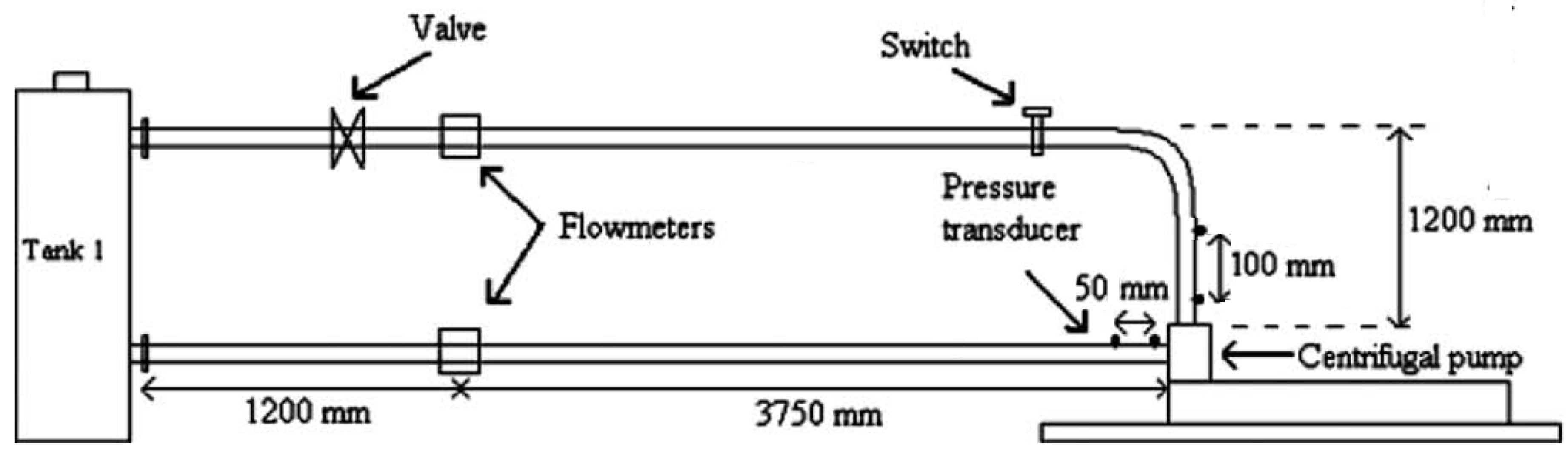
2.1. Description of the Facility

The DERAP test loop set at the LMFL allows two configurations: a closed circuit with the suction and delivery pipes connected to a single tank and an open circuit with two separate tanks, whose pressures can be set independently. A valve is used to switch from one to the other. The closed configuration has been used for the startup experiments simulated here. Pressure is imposed at the top of the tank (see Figure 1). A control valve is located on the delivery pipe, whose purpose is to control the flow rate by changing the global circuit pressure loss.

Two pressure transducers are used on the test rig: one 50 mm upstream of the impeller on the suction pipe and another 100 mm downstream on the delivery pipe. Duplaa [15] conducted single-phase and two-phase cavitating fast startups. Single-phase conditions were obtained by imposing a sufficient pressure in the tank to avoid cavitation (2.8 bars). Results of the simulation of this single-phase test are presented in the following sections.

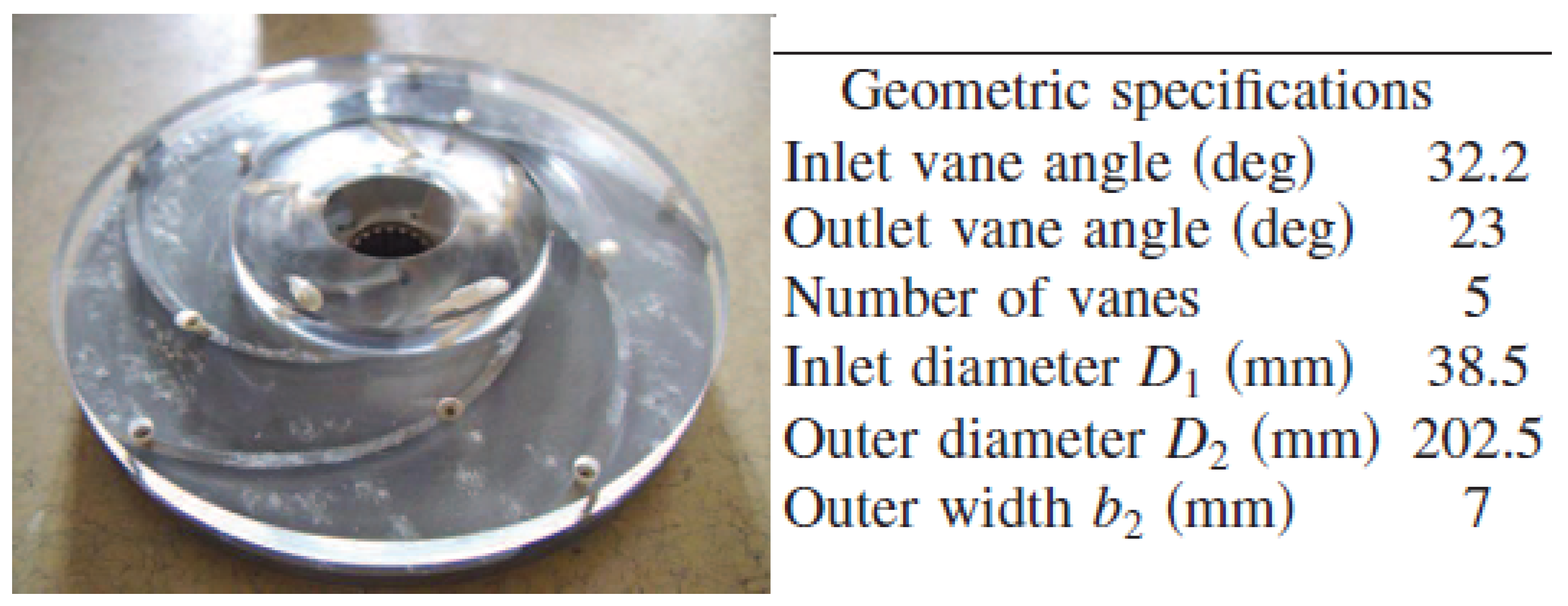
2.2. Description of the Centrifugal Pump of the DERAP Loop

The centrifugal pump—called DERAP—has been set at the LMFL to study the pump behaviour in cavitating and non-cavitating operating conditions during fast startups. It was the support of the successive works of Ghelici [16,17], Picavet [18,19,20], Bolpaire [21,22,23] and Duplaa [15,24,25]. Measurements have been conducted in single-phase and two-phase cavitating conditions in steady and transient regimes. The pump has been operated only in the first quadrant (positive rotational speed and flow rate).

The DERAP impeller is shown in Figure 2 and Figure 3. The expected nominal point of the DERAP centrifugal pump at the design stage was $Q_N=23$ m³/h, $H_N=50$ m and $N_N=2900$ rpm, which led to a specific speed of $12.3$ according to the common European definition of specific speed $N_q=\frac{N\sqrt{Q}}{H^{3/4}}$ (Gülich [26]). Experimentation of the pump led to a reconsideration of the nominal point as $Q_N=23$ m³/h, $H_N=42.8$ m and $N_N=2900$ rpm, which is used in the following simulations.

A vaneless diffuser of constant width (7 mm), whose inlet and outlet diameters are, respectively, 206 and 240 mm, is located downstream the impeller. A simple diverging volute is located downstream the diffuser, as shown in Figure 4, and is then connected to the discharge pipe. More information on DERAP pump geometric data is available in the work of Duplaa [15]. In the present study, only single-phase characteristics are used to qualify the predictive 1D-pump model. The two-phase measurements will be used in a further study dedicated to two-phase qualification of the model.

3. Modelling of the Pump and the Complete Circuit

3.1. The CATHARE-3 Code and Its Governing Equations

CATHARE-3 is a French two-phase flow modular system code. It has been owned and developed since 1979 by CEA and its partners EDF, Framatome and Institut de Radioprotection et de Sûreté Nucléaire (IRSN). Barre and Bernard [27] reported more details on the code development and validation strategy.

One-dimensional (1D), three-dimensional (3D) or point (0D) hydraulic elements can be associated together to represent a whole facility. They, respectively, correspond to one or three directions allowed for the fluid, and to components where fluid velocity is negligible such as capacities. Thermal and hydraulic submodules (e.g., warming walls, valves, pumps and turbines) can be added to main hydraulic elements to, respectively, take into account thermal transfer, flow limitation, pressure rise or pressure drop. Six local and instantaneous balance equations (mass, momentum and energy for each phase) make possible liquid and gas representation for transient calculations. Mechanical and thermal disequilibria between phases can thus be represented (cf. Faydide and Rousseau [28]). Time and space phase average induces the use of physical closure laws in the balance equations system (Bestion [29]).

Resolution is made using a implicit scheme which allows large variations of the time step during the computation and low CPU time cost. The governing equations discretised for the 1D module are given below. The 1D mesh allows one direction for liquid and gas velocities but two possible ways (positive or negative). z and k, respectively, correspond to the curvilinear abscissa and the phase index (k = L for the liquid and k = G for the gas).

Phase mass balance:

$$\frac{\partial }{\partial t}A{\alpha }_k{\rho }_k + \frac{\partial }{\partial z}A{\alpha }_k{\rho }_k{V}_k = {ϵ}_{k}A\Gamma + S_k$$

(1)

Phase momentum balance:

$$\begin{array}{r}\frac{\partial }{\partial t}A{\alpha }_k{\rho }_k{V}_k+{\displaystyle \frac{\partial }{\partial z}}A{\alpha }_k{\rho }_k{V}_k^2+A{\alpha }_k{\displaystyle \frac{\partial P}{\partial z}}+A{p}_i{\displaystyle \frac{\partial {\alpha }_k}{\partial z}}\\ +A{ϵ}_k\beta \alpha (1-\alpha ){\rho }_m\left[{\displaystyle \frac{\partial V_G}{\partial t}}-{\displaystyle \frac{\partial V_L}{\partial t}}+V_G{\displaystyle \frac{\partial V_G}{\partial z}}-V_L{\displaystyle \frac{\partial V_L}{\partial z}}\right]\\ =A{ϵ}_k\Gamma W_i-A{ϵ}_k{\tau }_i-(C_k{\chi }_f+{\displaystyle \frac{AK{\alpha }_k}{\Delta z}}){\tau }_k\\ +A{\alpha }_k{\rho }_k{g}_z+{\displaystyle \frac{R(1-{\alpha }_k)}{4}}{p}_i{\displaystyle \frac{\partial A}{\partial z}}+S{M}_k\end{array}$$

(2)

Phase energy balance:

$$\begin{array}{r}\frac{\partial }{\partial t}\left[A{\alpha }_k{\rho }_k(h_k+\frac{V_k^2}{2})\right]+{\displaystyle \frac{\partial }{\partial z}}\left[A{\alpha }_k{\rho }_k{V}_k(h_k+\frac{V_k^2}{2})\right]-A{\alpha }_k{\displaystyle \frac{\partial P}{\partial t}}\\ =+A{\alpha }_k{\rho }_k{V}_k{g}_z+{\chi }_c{q}_{w,k}+A{q}_{k,E}+A{ϵ}_k\Gamma (h_k+\frac{W_i^2}{2})+S{E}_k\end{array}$$

(3)

Mass transfer term:

$$\Gamma =\frac{{\chi }_c/A{q}_{w,i}-q_{L,i}-q_{V,i}}{h_V-h_L}$$

(4)

Equations (1)–(3) are solved for each phase (liquid and gas) in classical CATHARE-3 computations. A six-equation local instantaneous system is thus obtained to represent two-phase flows in experimental loops or whole nuclear reactors. See the work of Bestion [29] for the description of each source term of the balance equations.

3.2. The One-Dimensional Pump Model Implemented into the CATHARE-3 Code

3.2.1. Principle

Flow inside parts of the pump (suction, impeller, diffuser and volute) is computed according to a one-dimensional discretisation following a mean flow path, as represented, respectively, in Figure 5 and Figure 6 for the case of the impeller and the diffuser parts.

In the impeller, the mean flow path is defined by the evolution of the mean relative angle $\beta$ from the impeller inlet to the outlet. The local relative angle $\beta$ of the cell is calculated assuming that $\sin \left(\beta \right(I\left)\right)$ is a linear function of the cell number I.

The mean flow path supposed to be followed by the fluid in the vaneless diffuser is a logarithmic spiral. This assumption corresponds to constant absolute angle $\alpha$ in the vaneless diffuser (Dou [30], Stanitz [31]).

3.2.2. Source Terms and Implementation

Adapting the CATHARE-3 bi-fluid model to a rotating frame resolution in order to simulate a rotodynamic pump resulted in significant code developments. The following adjunctions or modifications to the standard CATHARE-3 1D-elements have been introduced to create a 1D-pump model, and especially to take into account the rotation effects, fluid deviation and losses:

• Inside the impeller, resolution is made with respect to the rotating frame ($W_k$ relative velocity replaces $V_k$ absolute velocity in each balance equation).
• A centrifugal acceleration term has been added to the right side of momentum balance equation of the impeller part. Its expression is the following:

  $$+A{\alpha }_k{\rho }_k{\omega }^{2}R\frac{\partial R}{\partial z}$$

  (5)
  It has also been introduced on the right side of energy balance equation as follows:

  $$+A{\alpha }_k{\rho }_k{W}_k{\omega }^2\frac{\partial R}{\partial z}$$

  (6)
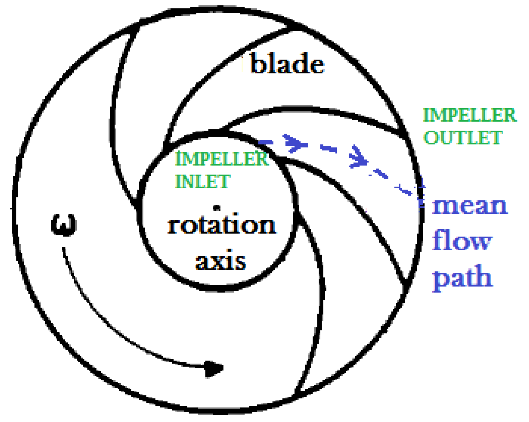
• Changes of frame are made at impeller and diffuser inlets using velocity triangles according to a mean velocity of the two-phase mixture. In the case of single-phase computations, this means velocity is simply the phase velocity.
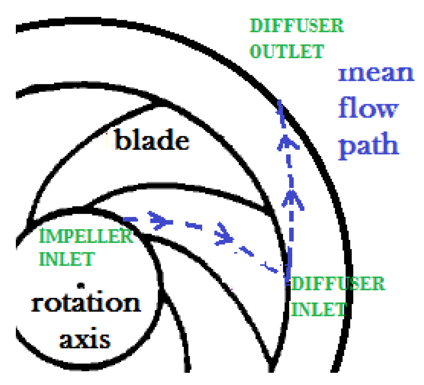
• Flow section is modified inside impeller, diffuser and volute parts in order to solve equations with the appropriate velocity (relative or absolute two-component velocity) and ensure mass flow rate conservation. Taking the example of the impeller part, the face number 1 is shared between suction and impeller. This correspond to the last point calculated in the absolute frame, as a face is the interface between two cells of the mesh. I is the face number, S the modified flow section and A the meridian flow section.

  $$S_{imp}(I=1)=A\left(1\right)$$

  (7)
  The change of frame is made on face number 2, owned only by the impeller part. The relative velocity at the impeller inlet $W\left(1\right)$ is estimated according to the inlet velocity triangle, which allows calculating a modified section, which replaces the initial meridian flow section in the balance equations.

  $$S_{imp}(I=2)=A\left(2\right)\frac{V_1}{W_1}$$

  (8)

  $$S_{imp}(I>2)=A\left(I\right)\sin \left(\beta \left(I\right)\right)$$

  (9)
  The same procedure is conducted for the change of frame from the relative to the absolute one. Thus, the flow section of the first face of the vaneless diffuser is the one of the impeller outlet.

  $$S_{dif}(I=1)=S_{imp}\left(I_{impeller outlet}\right)=S_{imp}\left(I_{io}\right)$$

  (10)
  The change of frame is made on face number 2, owned only by the diffuser-volute element part (see Figure 7 for the representation of this element). The two-component absolute velocity at the diffuser inlet $\overrightarrow{V\left(1\right)}=\overrightarrow{V_T\left(1\right)}+\overrightarrow{V_m\left(1\right)}$ is estimated according to the outlet velocity triangle, which allows calculating a modified flow section as follows:

  $$S_{dif}(I=2)=S_{imp}\left(I_{io}\right)\frac{W_2}{V_2}$$

  (11)

  $$S_{dif}(I>2)=A\left(I\right)\sin \left(\alpha \left(I\right)\right)$$

  (12)
• Flow direction in the vaneless diffuser is modelled considering a constant absolute angle along the diffuser mesh. This corresponds to a logarithmic spiral path.

  $$\alpha \left(I\right)={\alpha }_2$$

  (13)
• Direction of the fluid along the volute is given by the evolution of the absolute angle $\alpha$. The flow is straightened in this component, which is essential to return to a one-component velocity in the downstream elements of the circuit (the discharge pipe in particular). The following relation defines the local absolute angle for each cell of the mesh:

  $$\sin \left(\alpha \left(I\right)\right)=\sin \left({\alpha }_2\right)+(\sin (\pi /2)-\sin \left({\alpha }_2\right))\frac{{(z\left(I\right)-z_4)}^2}{{(z_6-z_4)}^2}$$

  (14)
• Conservation of the static pressure and static enthalpies is ensured at frame interfaces. This allows working with the relative total pressure and enthalpies in the rotating frame.
• Fluid deviation at impeller outlet is taken into account by a slip factor model. It represents Coriolis acceleration effects in particular. Several correlations have been implemented, including those of Stodola [32], Stanitz [33], Wiesner [34] and Qiu [35] as well as the one developed in the frame of this project (Matteo et al [13]) activated by default and used for qualification of the pump model. These correlations are presented in the next section. After making the choice of the slip factor model (i.e., a correlation for $\sigma$), the deviated angle is calculated as follows:

  $$F_{dev}=\frac{\alpha }{\max (\nu ,{\nu }_{lim})}{\displaystyle \frac{{\omega }_N}{Q_N}}{R}_2{A}_2(1-\sigma )$$

  (15)

  with ${\nu }_{lim}=5.{10}^{-2}$

  $${\beta }_2^{\prime }=arctan\left({\displaystyle \frac{1}{\frac{\cos \left({\beta }_2\right)}{\sin \left({\beta }_2\right)}+F_{dev}}}\right)$$

  (16)
• A desadaptation (shock) head loss source term has been added to the right side of momentum equations. It is concentrated at the impeller inlet using the repartition function $r_i$.

  $$-A{\alpha }_k{\rho }_{k}g{\Delta H}_{shock}\frac{r_i}{\Delta z}$$

  (17)
• A diffusion head loss source term has been added to the right side of momentum equations of the volute part. It is spread all along the volute mesh using the repartition function $r_i$.

  $$-A{\alpha }_k{\rho }_{k}g{\Delta H}_{diffusion}\frac{r_i}{\Delta z}$$

  (18)
• Power dissipation in the fluid due to low flow rate recirculations has been introduced into energy balance equations. It is spread all along the impeller mesh using the repartition function $r_i$.

  $$+{\alpha }_k{\rho }_k{\Gamma }_{dissipation}.\left|\omega \right|\frac{r_i}{\Delta z}$$

  (19)

Friction losses are already taken into account by the standard 1D pipe model of the CATHARE-3 code. They are calculated according to the Zigrang and Sylvester correlation [36] in each mesh cell. The friction perimeter and the absolute rugosity of the pump parts have to be provided to compute correctly these losses.

3.2.3. Deviation and Loss Models

Several slip factor correlations have been implemented in the 1D pump model in order to make sensitivity studies and evaluate qualities and defaults of each (those of Stodola [32], Stanitz [33], Wiesner [34] and Qiu [35] as well as the one developed in the frame of this project). These correlations have been tested on four centrifugal pumps, two mixed flow pumps and one radial compressor (Matteo et al. [8,9,10,11,12,13]). The correlations are described here after.

Stodola’s slip factor model [32]:

$${\sigma }_{Stodola}=1-\frac{\pi \sin \left({\beta }_2\right)}{Z}$$

(20)

Stanitz’s slip factor model [33]:

$${\sigma }_{Stanitz}=1-\frac{0.63\pi }{Z}$$

(21)

Wiesner’s slip factor model [34]:

$${\sigma }_{Wiesner}=1-\frac{\sqrt{\sin \left({\beta }_2\right)}}{Z^{0.7}}\hspace{1em}if\hspace{1em}\frac{R_1}{R_2}\le {ϵ}_{lim}$$

(22)

$${\sigma }_{Wiesner}=\left(1-\frac{\sqrt{\sin \left({\beta }_2\right)}}{Z^{0.7}}\right)\left(1-{\left(\frac{\frac{R_1}{R_2}-{ϵ}_{lim}}{1-{ϵ}_{lim}}\right)}^3\right)\hspace{1em}else$$

(23)

$$with {ϵ}_{lim}=exp(-\frac{8.16.\sin \left({\beta }_2\right)}{Z})$$

(24)

Qiu’s slip factor model [35]:

$${\sigma }_{Qiu}=1-\frac{F\pi \sin \left({\beta }_2\right)\cos \left({\gamma }_2\right)}{Z_2}-\frac{F{s}_2{\Phi }_2}{4\sin \left({\beta }_2\right)}{\left(\frac{d\beta }{dm}\right)}_2+\frac{F{\Phi }_2{s}_2\cos \left({\beta }_2\right)}{4{\rho }_2{b}_2}{\left(\frac{d\rho b}{dm}\right)}_2$$

(25)

which can be expressed as a sum of several terms:

$${\sigma }_{Qiu}=1-\Delta {\sigma }_{radial}-\Delta {\sigma }_{turn}-\Delta {\sigma }_{passage}$$

(26)

F function, which is involved in ${\sigma }_{Qiu}$, is written as follows:

$$F=1-\sin \frac{\pi }{Z_2}\sin \left(\frac{\pi }{Z_2}+(\frac{\pi }{2}-{\beta }_2)\right)\sin \left({\beta }_2\right)\cos \left({\gamma }_2\right)-\frac{t_2}{s_2\sin \left({\beta }_2\right)}$$

(27)

Qiu’s model [35] is valid while $\frac{R_1}{R_2}<F$.

Slip factor model developed in the frame of this work (Matteo et al. [13]):

$${\sigma }_{present work}=1-\frac{\pi \sin \left({\beta }_2\right)\cos \left({\gamma }_2\right)}{Z}$$

(28)

Stodola’s and Wiesner’s slip factor models are both references in the domain. Stodola’s model [32] is a reference because it is the oldest (1927) and first mechanistic model that still gives reasonably satisfactory results. Wiesner’s model [34] (1967), which is an empirical model, is a reference because it has been developed according to a large range of pump geometries and often gives good results. Other authors investigated the slip factor modelling, more or less recently, such as Stanitz [33] in 1952, Pfleiderer [37] in 1961, Eck [38] in 1972, Paeng and Chung [39] in 2001 and Qiu [35] in 2011. Qiu’s model seems to give good results according to the literature (Dixon and Hall [40]), even if its expression is more complicated and asking for more geometrical input data. The necessity to propose a slip factor correlation in the frame of this work appeared when trying to model mixed flow pumps (Matteo et al. [13]). To answer this need, a generalisation of Stodola’s correlation in the case of mixed-flow pumps has been proposed. The corresponding correlation is called “present work” in the following. For a simple radial pump such as the one modelled in the present paper, both Stodola’s and “present work” correlations are equivalent (see Figures 9 and 10).

Loss models specific to a pump geometry (shock and diffusion head losses, and power dissipation due to recirculations) are implemented as described hereafter.

First, the desadaptation coefficient D is calculated as:

$$D=\frac{Q}{Q_N.\max (\frac{\omega }{{\omega }_N},{\alpha }_{lim})}$$

(29)

with ${\alpha }_{lim}=7.{10}^{-7}$

Then, the shock head loss model for the low flow rates ($D<1$) is expressed as:

$${\Delta H}_{shock}={\Delta H}_{shock,0} {(D-1)}^2$$

(30)

with ${\Delta H}_{shock,0}=H_{Euler,0}-H_0$. The choice that is made here consists in modelling the difference between the homologous head at zero flow rate estimated by the Euler equation taking into account the deviation $H_{Euler,0}$ and the real value $H_0$. Shock losses are assumed to be the only phenomenon explaining this difference near the zero flow rate.

$H_{Euler,0}$ is estimated as $75\%.{U_2}^2/g$.

$H_0$ depends on the specific speed $N_q$ and is expressed as:

$$H_0=(K_1.N_q+K_2){\left(\max (\frac{\omega }{{\omega }_N},{\alpha }_{lim})\right)}^2{H}_N$$

(31)

with $K_1=7.{10}^{-3}$ and $K_2=1.0092$. These coefficients have been defined by studying four-quadrant characteristics of several rotodynamic pumps.

The flow direction is assumed to be adapted to the blades at $D=1$, and consequently ${\Delta H}_{shock}=0$. Continuity between low and high flow rate conditions is ensured by the correlations.

The shock head loss model for the high flow rates ($D>1$) is expressed as:

$${\Delta H}_{shock}={\Delta H}_{shock,\infty } {(D-1)}^2$$

(32)

$${\Delta H}_{shock,\infty }=K_3.\max (\frac{N_q}{70},1){\left(\max (\frac{\omega }{{\omega }_N},{\alpha }_{lim})\right)}^2{H}_N$$

(33)

with $K_3=7.5.{10}^{-1}$.

The diffusion head loss model, representing losses due to the diverging flow section in the volute, is expressed as follows:

$${\Delta H}_{diffusion}=K_{4}D{\left(\max (\frac{\omega }{{\omega }_N},{\alpha }_{lim})\right)}^2\frac{{(V_{T,3}-V_6)}^2}{2}$$

(34)

with $K_4=0.65$

Finally, the power losses due to recirculations at low flow rate are expressed as follows:

$${\Gamma }_{dissipation}={\beta }_0{\Gamma }_N{\left(\max (\frac{\omega }{{\omega }_N},{\alpha }_{lim})\right)}^2{\left(\frac{D-b_3}{b_3}\right)}^2$$

(35)

for $D\le b_3=\frac{1}{2}$, and 0 otherwise. ${\beta }_0=b_1.N_q+b_2$ with $b_1=6.6.{10}^{-3}$ and $b_2=2.055.{10}^{-1}$.

These losses specific to a pump geometry are located along the mesh of the impeller and the volute elements. To make the developed pump model general, non-dimensional quantities, such as the specific speed and the rotational speed ratio, have been introduced into the coefficients of the loss models. A limit of the rotational speed ratio $\frac{\omega }{{\omega }_N}$ has been introduced in relation with the work conducted on locked rotor situations (Matteo et al. [12,13]).

3.2.4. Required Input Data

Required input data can be separated into three types: general, geometric and hydraulic data.

General Data

The nominal point of the pump ($Q_N$, $H_N$ and $N_N$) has to be defined. If the rotational speed has to be computed with the turning mass equation, then inertia, friction torque and synchronism velocity have to be provided. Otherwise, a time-dependent law has to be imposed.

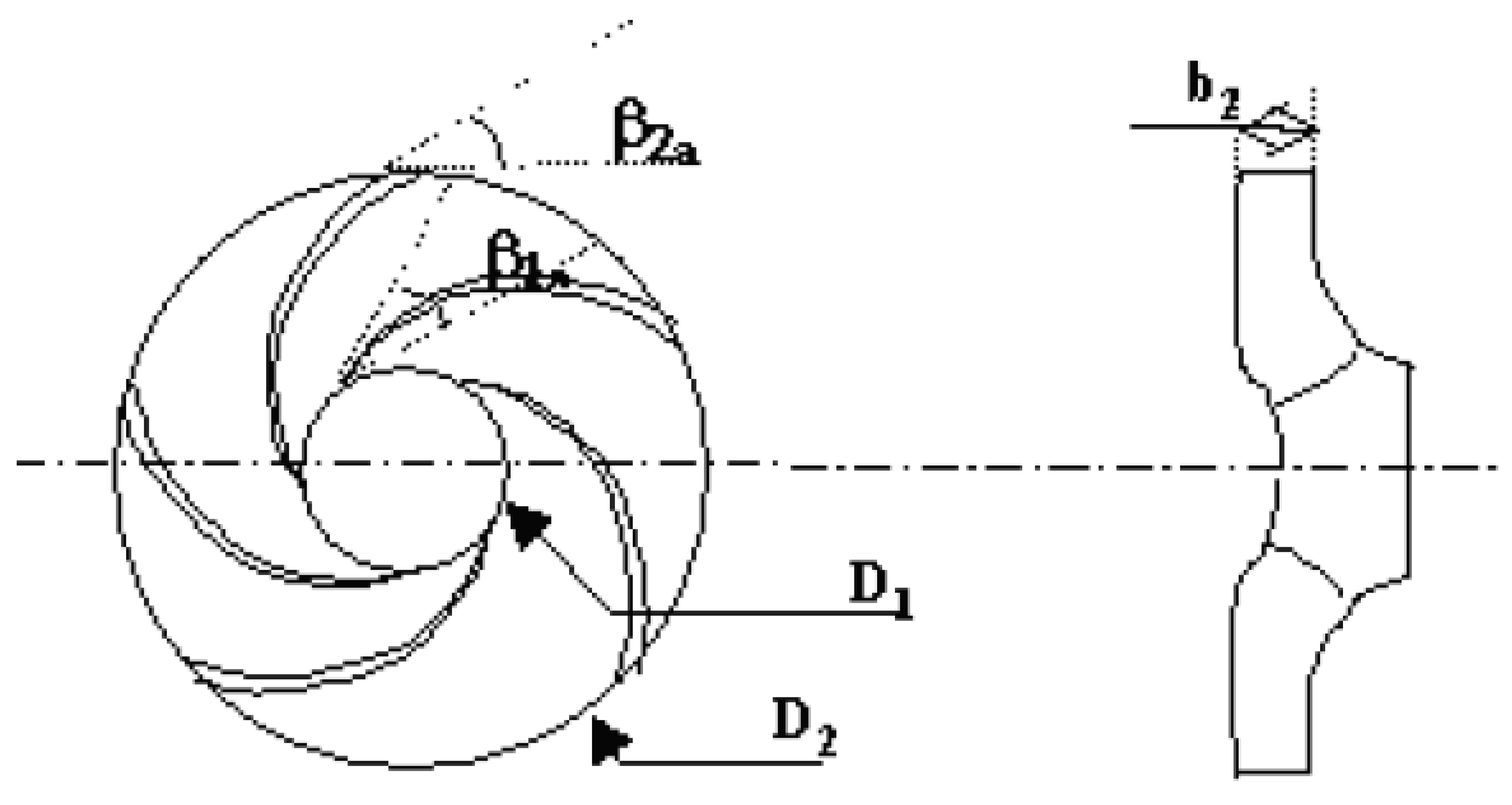
Geometric Data

For the impeller part only: hub and tip radius and blade angles ($\beta$) at inlet and outlet have to be introduced, and also the number of blades.

The length of each element (following the curvilinear abscissa) and their orientation have to be provided. The impeller length is determined in relation with the computed outlet radius (via integration of $\frac{\partial R}{\partial z}=cos\left(\gamma \right)sin\left(\beta \right)$ along the impeller). The diffuser length corresponds to the logarithmic spiral path. The volute length corresponds to a calculated mean length. These lengths do not change during the computation. They correspond to the adapted flow situation. Off-design distortion of the path is taken into account by global effects in loss models. The meridian flow section, the friction perimeter and the rugosity along fixed and mobile elements have to be defined.

Hydraulic Data

In the case of pump-only computations, pressure (at the outlet boundary condition), temperature, flow rate and void fraction (at the inlet boundary condition) have to be imposed. For whole circuit modelling, these quantities are calculated with respect to the interaction between elements.

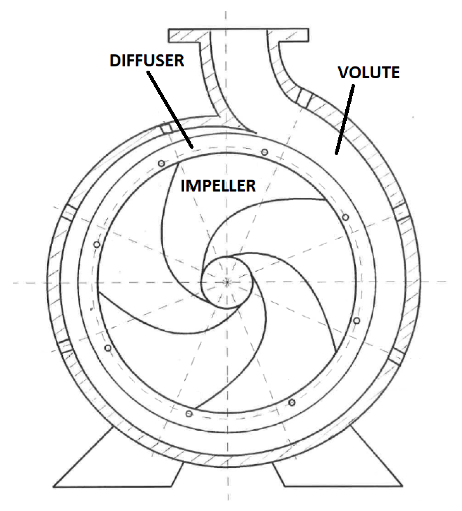
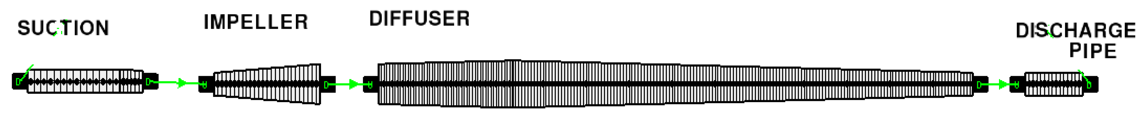
3.3. Graphic Representation of the Modelling

3.3.1. Centrifugal Pump

When modelling the DERAP low specific speed centrifugal pump using the CATHARE-3 1D-pump developed model, the representation shown in Figure 7 is obtained. Meridian flow sections are represented in this figure. Each part of the pump (suction, impeller, diffuser, volute and discharge pipe) is modelled using a one-dimensional element.

It is recommended to use comparable cell sizes along elements (ratio between cell length should not exceed 1.2 to avoid inappropriate averages in computations). Convergence of results has been tested by equally refining the pump mesh. The mesh that has been finally chosen corresponds to the coarser mesh allowing to obtain convergence of results (respectively, 20, 26, 200 and 15 cells for the suction pipe, the impeller, the diffuser + volute and the discharge pipe).

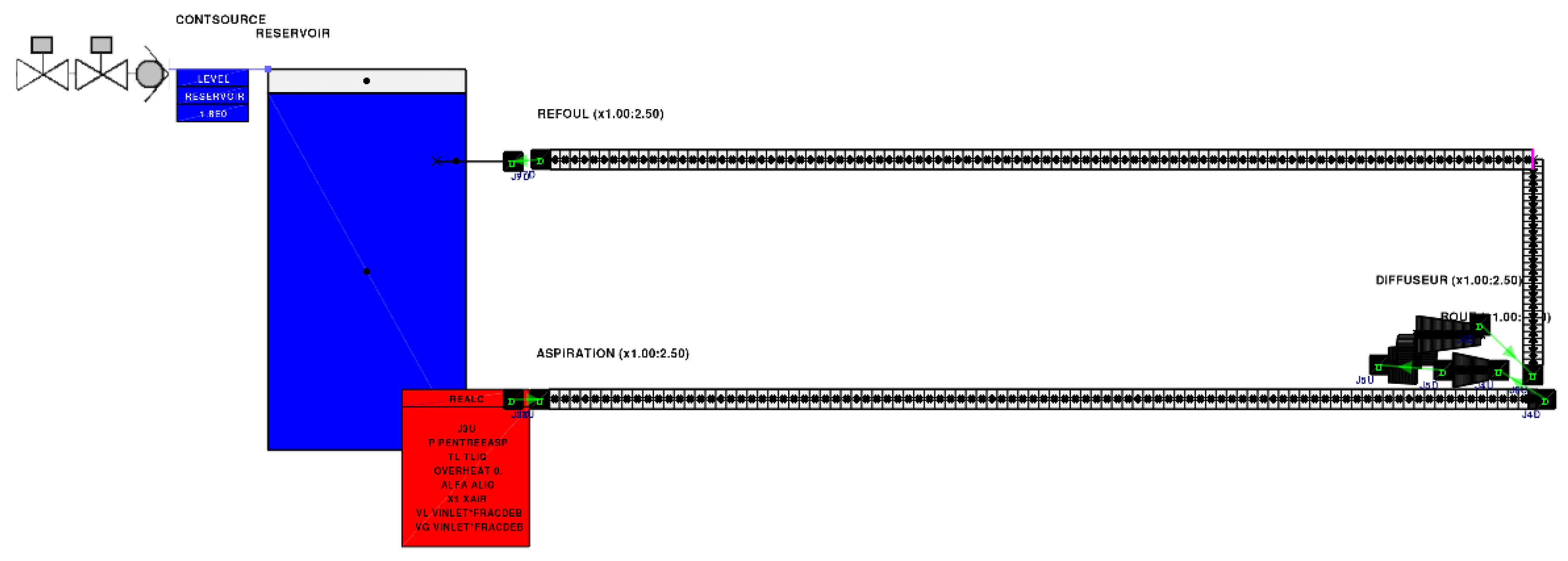
3.3.2. Whole Facility

The CATHARE-3 modelling of the circuit was done using 1D and 0D elements. Compared to Figure 7, the suction and delivery elements have been extended to represent the whole pipes of the DERAP loop. Two singular pressure loss coefficients are defined on the delivery pipe to take into account the elbow and the flow rate control valve, respectively.

The tank is a large fluid capacity with several connections, thus a 0D element has been used to represent it. Its two junctions are linked to the suction and delivery pipes (Figure 8).

The same geometry as the one used in the component scale data deck (Figure 7) is used for the impeller, diffuser and volute parts. Only the orientation of elements has been adapted. In particular, the volute outlet height of the experimental setup is respected in the simulation. These 1D elements are placed on the bottom right of Figure 8.

4. Results

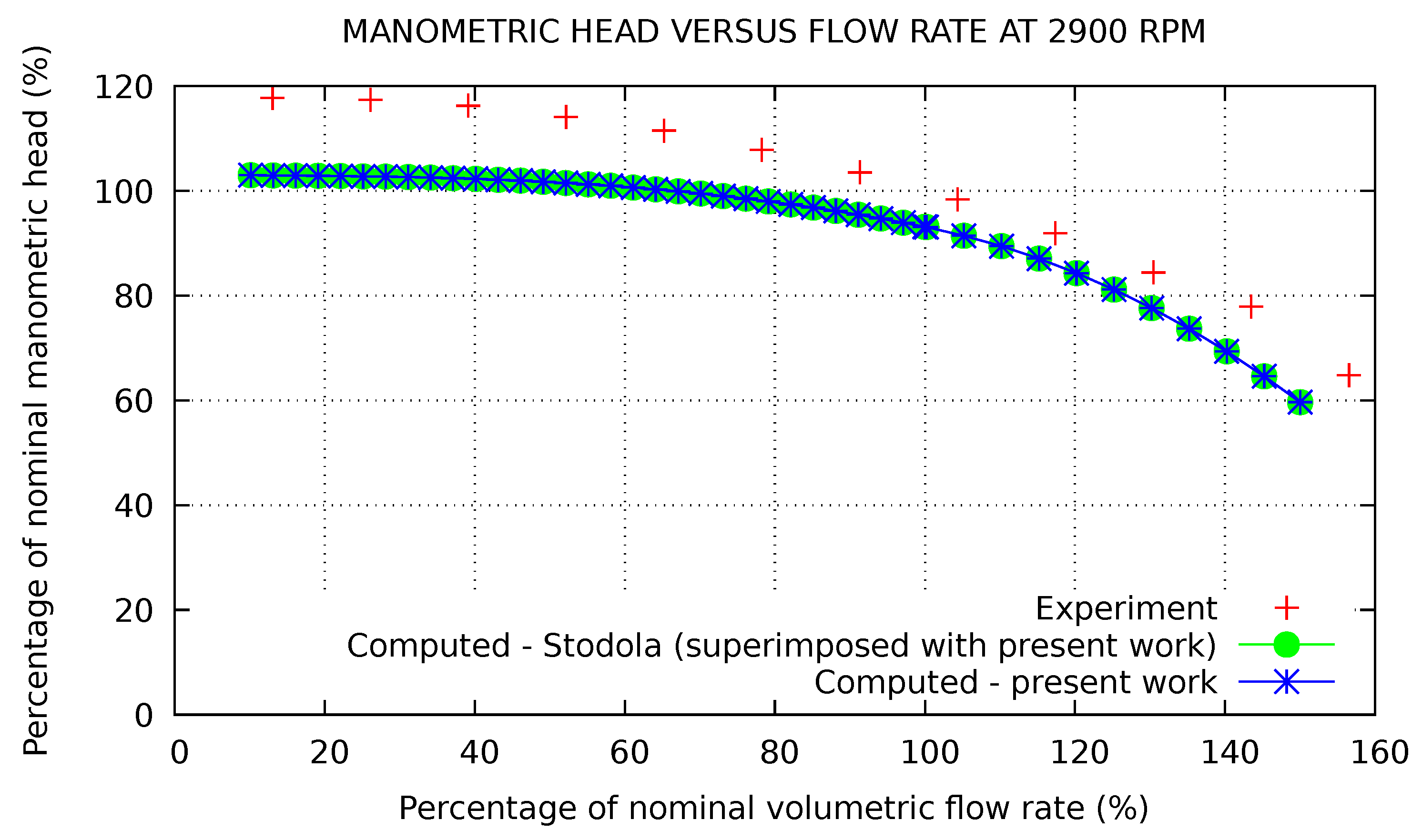
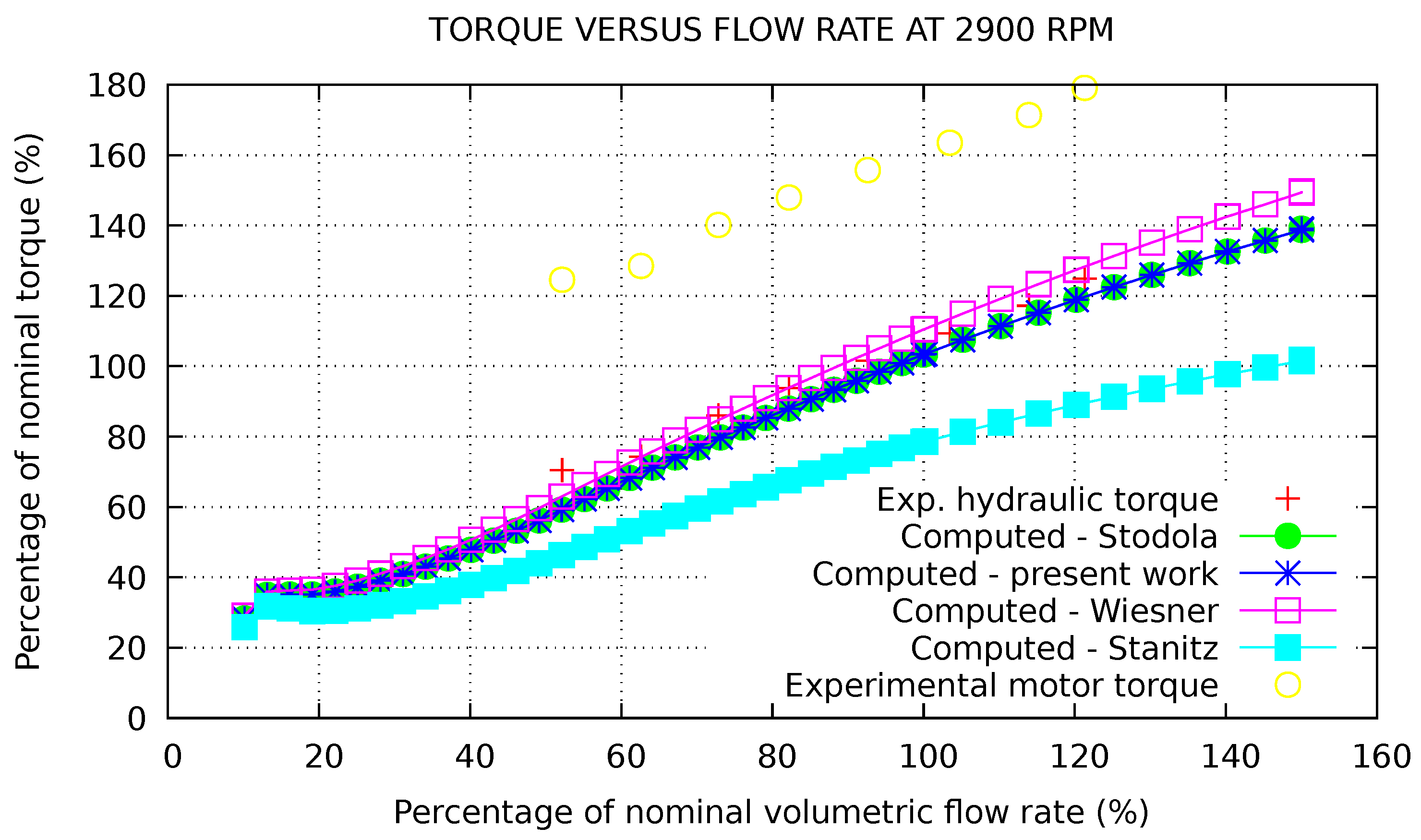
4.1. Prediction of DERAP Steady Performance Curves (Pump Only)

First, the prediction of steady performance curves of the DERAP centrifugal pump using the developed model is presented in the following. This is done to analyse the validity of the slip factor and loss models presented before. For this first step, the -pump-only modelling is used involving hydraulic boundary conditions.

To produce head and torque performance curves of the DERAP pump, a slow evolution (400-second long) of the flow rate (from $10\%$ to $150\%$) is imposed at the inlet boundary condition of the modelled pump while keeping a constant nominal rotational speed. Total CPU time of the computation is 6 s using one core of a classic desk machine, which is 67 times faster than the simulated time. Head and torque performance curves can be observed in Figure 9 and Figure 10.

In Figure 9, it can be seen that the total head of the pump is correctly predicted. The relative error (defined as the difference between the experimental and the computed head values, and divided by the experimental one $\frac{H_{exp}-H_{calc}}{H_{exp}}$) is less than 5% at the nominal operating point and does not exceed $13.6\%$ in the whole operating range. The maximal relative error is reached at a very low flow rate close to $30\%Q_N$. The strengths of the model are, first, to ensure such an order of error for very different geometries from radial to mixed flow machines ($10<N_q<120$) and from little to very large components (20 cm $<D_{impeller}<$150 cm), and, second, to predict these presented performance curves with a very low computation cost (6 s on one core of a standard computer) (see Matteo et al. [9,10,11,12,13]). Probabilistic studies can complete such a model by changing randomly parameters of the model and analysing the impact of uncertainties on the final results.

As mentioned above, as the slip factor correlation called ““present work”’ is a generalisation of Stodola’s one for mixed-flow pumps, both are superimposed in Figure 9 and Figure 10. It was expected in the case of the DERAP radial pump.

Experimental measurements provide a mechanical torque measured on the shaft, whereas the model predicts a hydraulic torque. Thus, the two values cannot be directly compared. However, assuming the friction torque as independent of flow rate (Duplaa [24]), they can be estimated at the nominal flow rate and removed on the whole flow rate range. It can be seen as an efficiency applied on the motor torque data to obtain an estimated experimental hydraulic torque, plotted in red cross in Figure 10, and which is very close to the value predicted by the model.

In the following, the modelling of the fast startup transient using the CATHARE-3 code is presented. Simulation results are compared to available transient experimental measurements.

4.2. Fast Startup Transient (Whole Circuit)

4.2.1. Description of the Transient

The experimental procedure conducted by Duplaa [15] was the following:

• The pump was started slowly to reach its nominal speed and then the flow control valve was adjusted to obtain the desired final flow rate.
• The pump was stopped and, after stabilisation of the circuit, the fast startup was launched.

In the computation, the flow control valve is modelled by a singular pressure drop, which is chosen to obtain the desired flow rate at the end of the startup transient. The experimental position of the flow control valve in the circuit is respected.

Similar to what was done in the experiment, pressure at the top of the tank is regulated at 2.8 bars to avoid cavitating conditions. The tank is full of liquid except at the very top where there is a free surface with compressed air above it. The pressure regulation in the simulation is done in the same way as in the experiment, using a gas injection/extraction valve. Injected gas is non-condensable air gas.

In the first 100 s of the CATHARE computation, the circuit is stabilised with a pump almost stopped. This means that a residual rotational speed ($2\%{\omega }_N$) is defined in order to initialise the circuit with a small flow rate, as $0\%$ flow rate computations are to be avoided for numerical resolution reasons.

The fast startup begins at 100 s and finishes at 101.5 s. Rotational speed evolution is imposed by a time dependent law. The aim of this validation work is to predict the flow rate, head (pressure difference) and torque evolutions and to compare it to available experimental data.

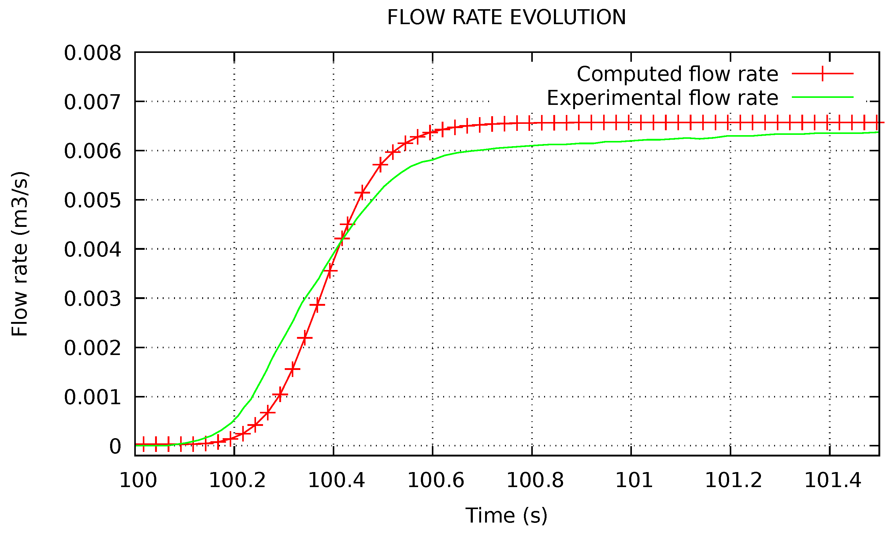
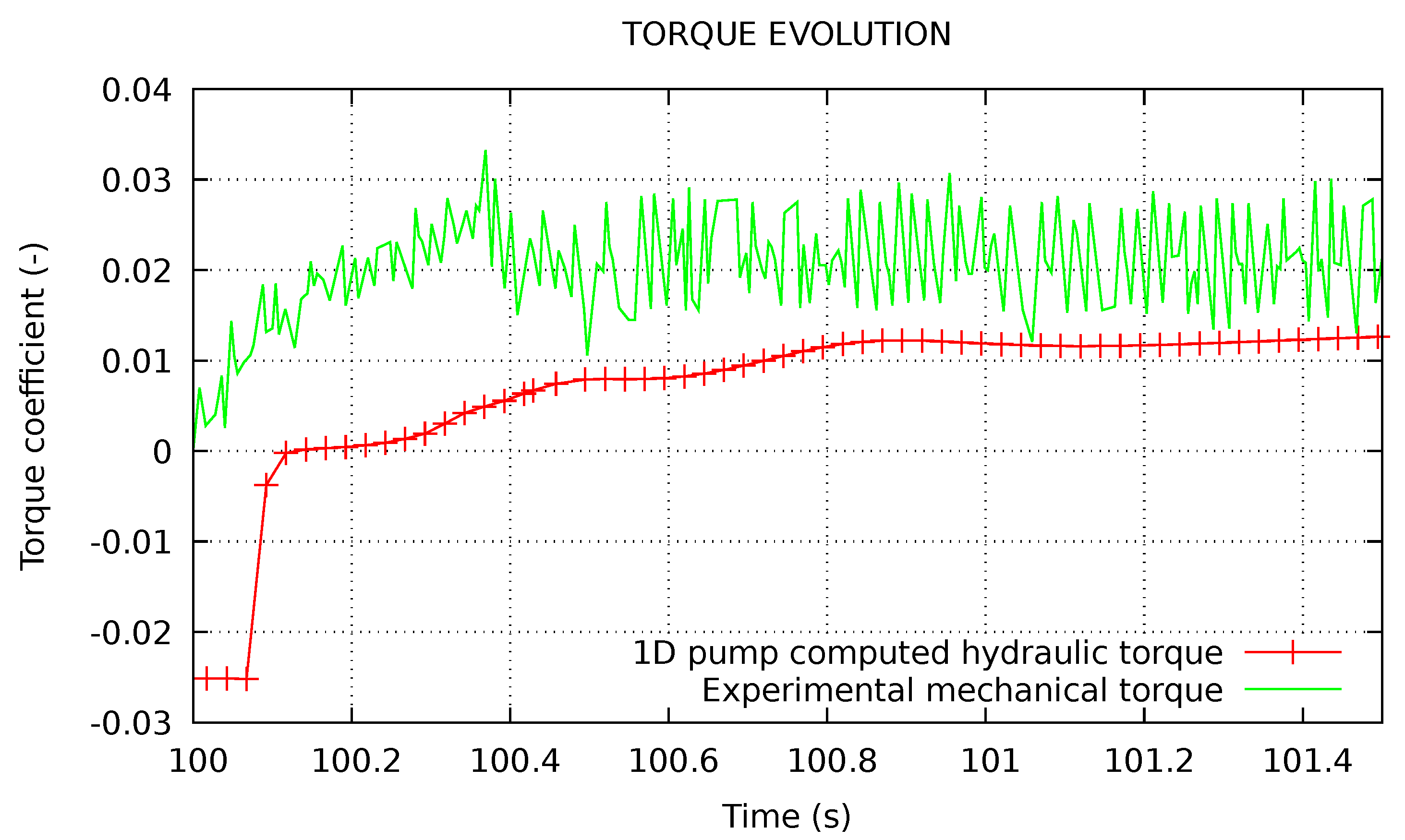
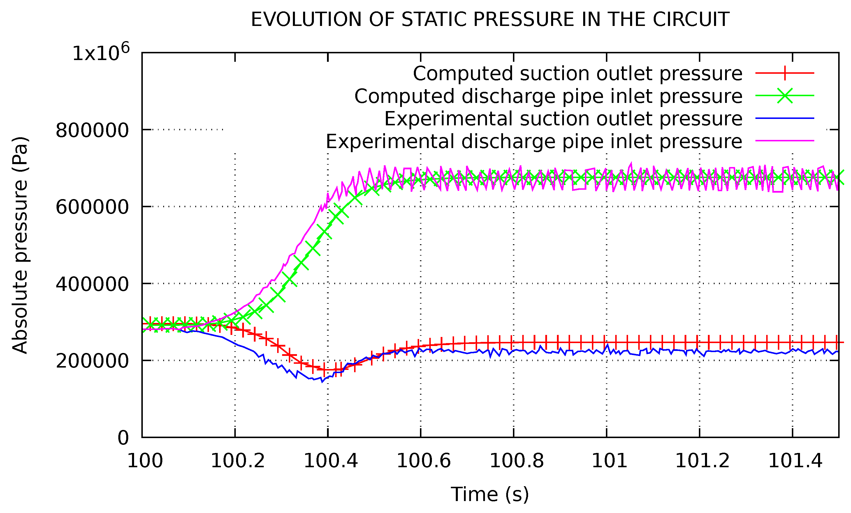
4.2.2. Evolution of Main Quantities During the Fast Startup

Predicted flow rate and pressure difference evolutions are, respectively, presented in Figure 11 and Figure 12. A good agreement is obtained when comparing predictions of the model to experimental data (a relative error less than 8% for flow rates higher than 50%$Q_N$ and increasing for low values of flow rate). Flow rate measurement uncertainties in such fast startup conditions are huge as the flow evolution is very difficult to capture and needs specific sensors. As a consequence, the differences observed between the predicted and the experimental flow rate evolutions are not significant.

Torque evolution is shown in Figure 13. Observable discrepancies are mostly due to the fact that the plotted experimental torque is a mechanical torque measured on the shaft, whereas the computed torque is a hydraulic torque. A peak of the measured motor torque can be observed before 100.4 s. This is due to the mechanical inertia of the motor, which is not taken into account in the model. Moreover, it can be seen that the hydraulic torque computed by the model before the startup (t = 100 s) is negative. This is due to the initial flow rate and rotational speed conditions that are not completely set to zero.

With the complete loop modelling, pressures can be analysed at different points in the circuit. In Figure 14, computed and experimental suction outlet pressure and discharge pipe inlet pressure are shown. It can be seen that pressure is rising at the discharge pipe inlet (this corresponds to the pump pressure rise) while it is dropping at the suction pipe outlet. The pressure dip before 100.6 s is caused by the flow inertia effects in the pipe. These two pressure evolutions are well predicted by the model by comparison to experimental pressure evolutions from Duplaa et al. [15].

The CATHARE code method seems to be adapted to simulate fast transients such as this startup. The robustness of the code was shown previously by simulating a transient affecting a High Temperature Gas Reactor turbine by Saez et al. [41] (but using another turbomachinery model of the CATHARE code).

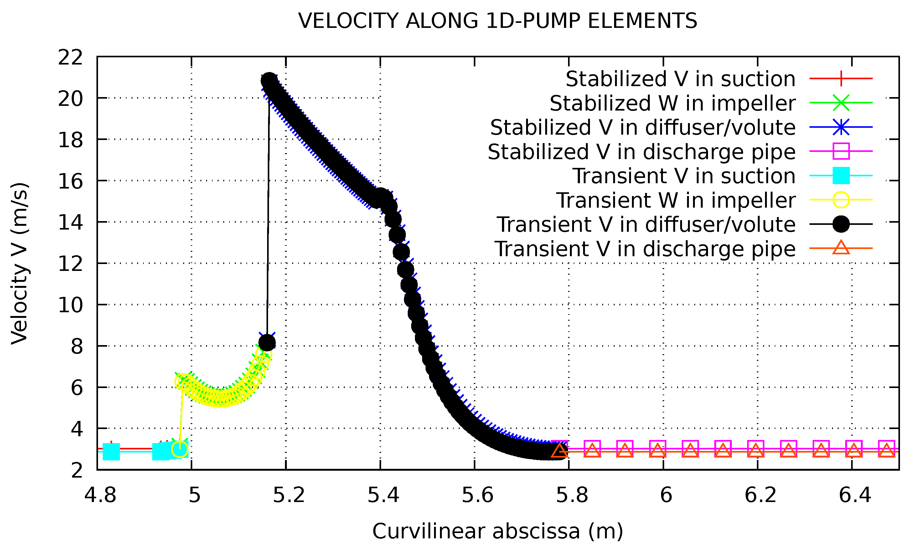
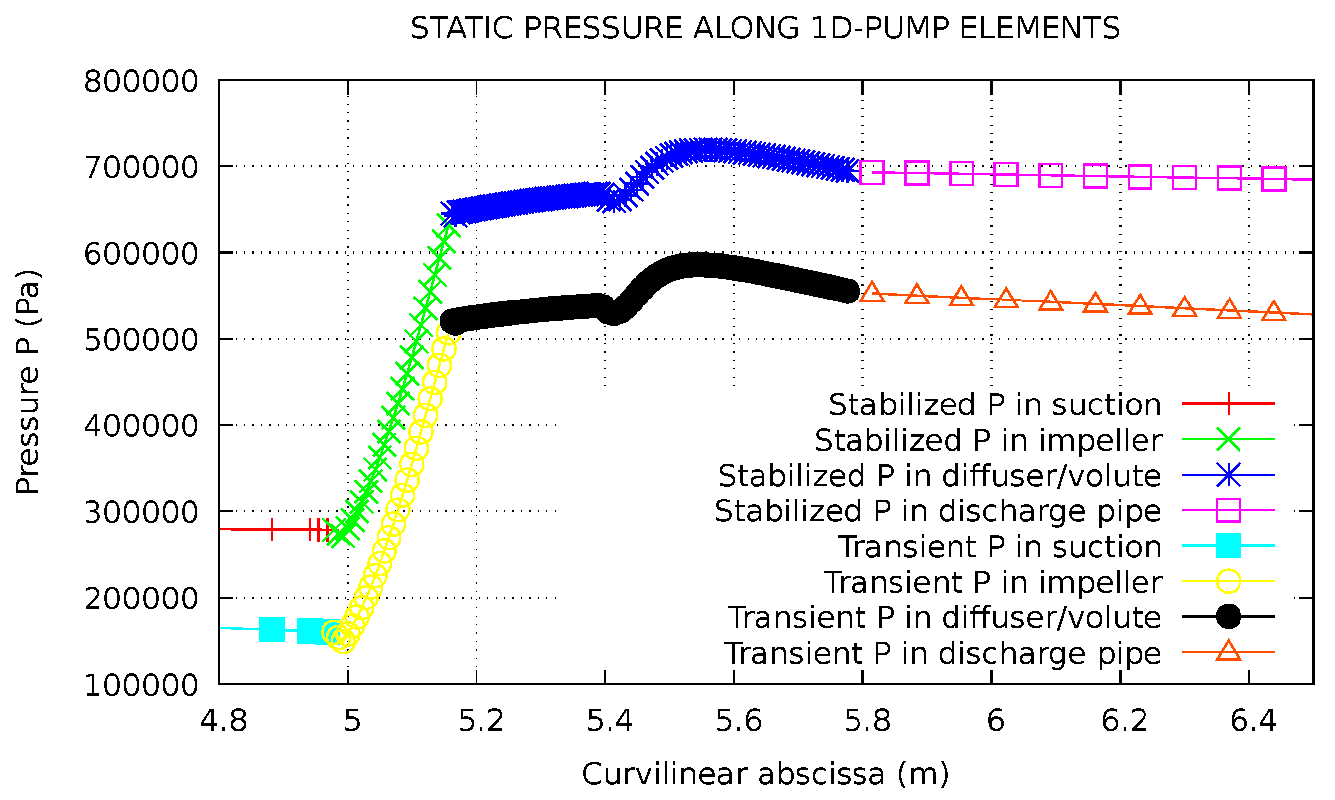
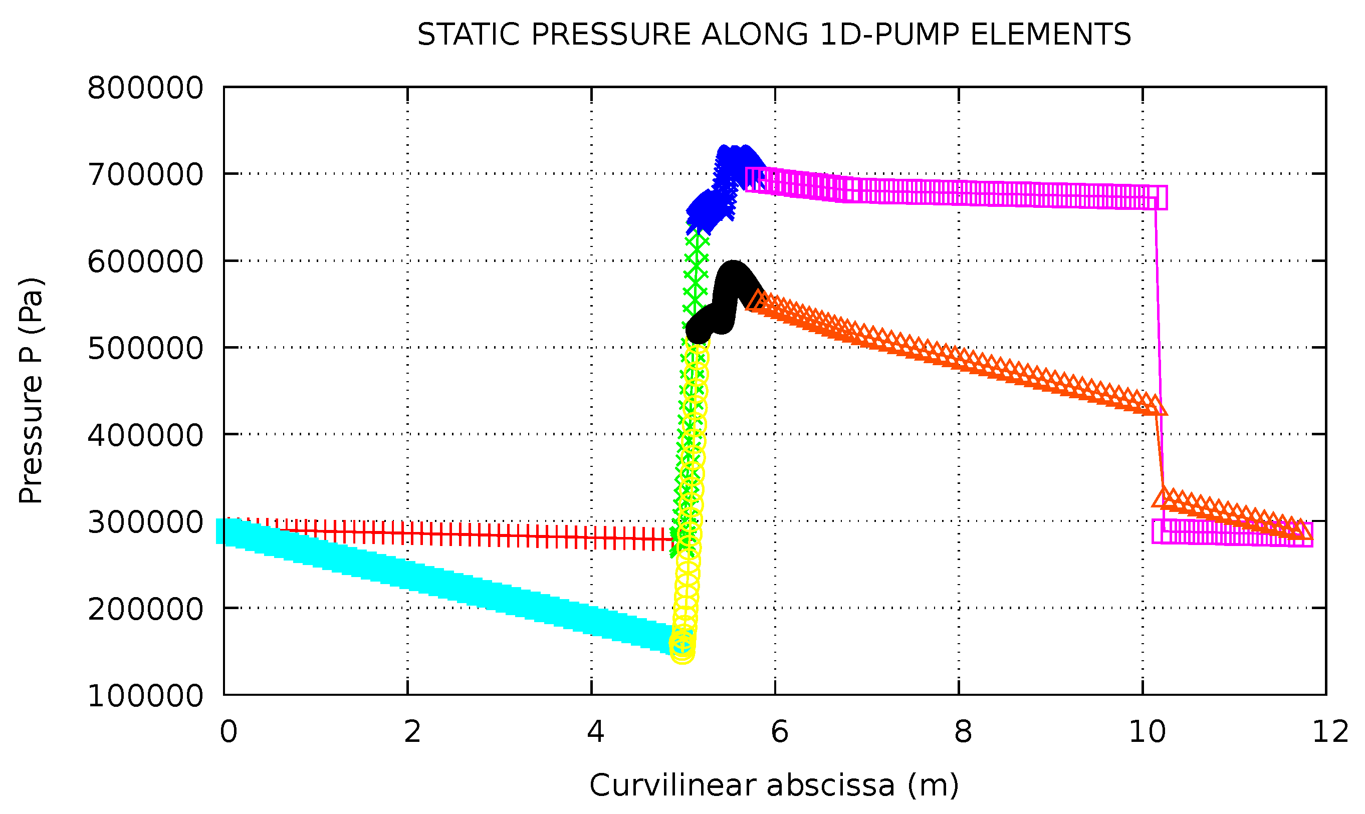
4.2.3. Pressure and Velocity Profiles Inside the Pump in Steady and Transient Conditions

One of the interests of the CATHARE-3 1D pump model is that profiles inside pump elements can be obtained during the computation. The aim of this part is to study the pressure and the velocity profiles inside the pump during the startup and in the equivalent steady regime (same flow rate and rotational speed but in stabilised conditions). To do this, quantities of interest are extracted at a chosen time during the startup. The time $t=100.4$ s is selected as it corresponds to a state where rotational speed and flow rate are still evolving ($\omega =90\%{\omega }_{end}$ and $Q=60\%Q_{end}$) and also where pressure at the suction outlet reaches its minimal value (see Figure 14).

At $t=100.4$ s of the startup, the rotational speed and the flow rate in the loop are, respectively, equal to 286 rad/s and $0.0038$ m³/s. To compare the behaviour of the circuit and of the pump in transient versus steady conditions, another simulation is conducted. The aim of this computation is to reach the same operating point and to stabilise the circuit in these conditions. To do this, the flow rate is regulated at the desired value by adapting the singular pressure drop representing the valve located on the discharge pipe. The pump is started slowly to reach the rotational speed equal to 286 rad/s.

In Figure 15 and Figure 16, velocity and static pressure profiles can be observed. It has to be noted that inside the rotating part (impeller) the velocity is the relative one, whereas it is the absolute one in the fixed parts (with only one axial component in the suction part, and with two components -axial and tangential- in the diffuser and volute parts). High velocities in the diffuser part can be observed, which cause friction losses. The flow direction evolves in the diffuser and volute parts. The absolute flow angle $\alpha$ (calculated towards the tangential direction) is gradually increased from its value at the diffuser outlet to $\frac{\pi }{2}$ according to a fitting as previously explained.

As explained above, the flow section is calculated depending on the local absolute angle along the diffuser and the volute according to the following relation: $S=S_m.\sin \left(\alpha \right)$.

The gap between the two pressure profiles of Figure 16 is due to the decrease of the suction outlet pressure during the startup, and especially observable at time $t=100.4$ s (see Figure 14). It can be seen, either in Figure 14 or in Figure 16, that a pressure of approximately 1.7 bars is reached at the suction outlet at this time. On the contrary, in the stabilised computation, inertial effects are no more observable and pressure is equal to 2.8 bars (situation comparable to the stabilised state after the startup in Figure 14).

These two different states of the circuit can be even better compared in Figure 17 where pressure profiles are plotted along the whole circuit. It can be seen that the tank is correctly regulating the pressure at 2.9 bars (it is located between the outlet of the discharge pipe at $z=12$ m and the suction inlet at $z=0$ m. However, pressure profiles in the long elements such as the suction and the discharge pipes are significantly different between steady and transient conditions.

Concerning the profiles inside the pump (Figure 16), they are very similar. It is also true concerning the velocity profiles inside the pump (Figure 15). No significant different behaviour of the machine is observed between steady and transient conditions. This shows clearly that transient effects of the whole circuit are dominant compared to transient effects of the pump. In the present case, this is due to the characteristic length of pipes, which is huge compared to the length of pump components. Using a shorter loop would certainly lead to reconsidering these conclusions.

5. Discussion

This paper presents a whole loop modelled with the CATHARE-3 thermal-hydraulic code. First, an original turbomachinery one-dimensional modelling approach following a mean flow path is presented. Correlations of the model are described and commented. The 1D modelling of the DERAP low specific speed centrifugal pump “alone” is then presented as well as the modelling of the complete circuit. Head and torque performances of the pump are compared to experimental ones. The agreement is satisfactory using this 1D approach as the relative error on the whole flow rate range tested is less than 10% for the total head and for a large range of operating points. Then, results obtained during a 1-s fast startup transient are analysed. With the complete loop modelling, it is possible to follow the evolution of several physical quantities of interest at different points of the circuit. This is done in the present study to analyse the evolution of pressure upstream and downstream from the pump, which allows observing the flow inertia effects in the loop. Finally, pressure and velocity profiles inside the pump and along the whole circuit are compared between transient and steady conditions. In the considered case of study, inertial effects of the global circuit are dominant when compared to pump inertial effects due to the high characteristic lengths of the pipes located around the machine.

This first validation at a loop system scale is a step bringing to analysis of reactor system scale response during hypothetical accidental transients of interest (pump seizure, pump stop on inertia, pump restart, cavitation occurring in working pumps, inverse flow rate and/or rotation speed, etc.). An additional validation using 1D/3D coupling, allowed by the CATHARE environment in which the model has been developed (Baviere et al. [42]), is considered in the future of this project. The objective would be to obtain some additional information about the flow characteristics in the pump to validate the evolution given in Figure 16. Moreover, one-phase computations are presented in this paper, but two-phase computations have started recently and another prospect is to validate the fast startup transient with cavitation occurring in the pump (see Duplaa [15] for experimental description of the two-phase tests).

References

- Chenaud, M.; Li, S.; Anderhuber, M.; Matteo, L.; Gerschenfeld, A. Computational thermal hydraulic schemes for SFR transient studies. In Proceedings of the NURETH-16, Chicago, IL, USA, 30 August–4 September 2015. [Google Scholar]
- Bouchard, J. GenIV International Forum 2007; Annual Report; OECD Nuclear Energy Agency: Paris, France, 2007. [Google Scholar]
- Varaine, F.; Marsault, P.; Chenaud, M.S.; Bernardin, B.; Conti, A.; Sciora, P.; Venard, C.; Fontaine, B.; Devictor, N.; Martin, L.; et al. Pre-conceptual design of ASTRID core. In Proceedings of the 2012 International Congress on Advances in Nuclear Power Plants-ICAPP’12, Chicago, IL, USA, 24–28 June 2012. [Google Scholar]
- Tenchine, D.; Pialla, D.; Gauthé, P.; Vasile, A. Natural convection test in Phenix reactor and associated CATHARE calculation. Nucl. Eng. Des. 2012, 253, 23–31. [Google Scholar] [CrossRef]
- Miettinen, J. Nuclear power plant simulators: Goals and evolution. In Proceedings of the Seminar on Transfer of Competence, Knowledge and Experience Gained through CSNI Activities in the Field of Thermal-Hydraulics (THICKET), Pisa, Italy, 5–9 May 2008. [Google Scholar]
- Mauger, G.; Bentivoglio, F.; Tauveron, N. Description of an improved turbomachinery model to be developed in the CATHARE-3 code for ASTRID power conversion system application. In Proceedings of the 16th International Topical Meeting on Nuclear Reactor Thermal Hydraulics (NURETH-16), Chicago, IL, USA, 30 August–4 September 2015. [Google Scholar]
- Mauger, G.; Tauveron, N.; Bentivoglio, F.; Ruby, A. On the dynamic modeling of Brayton cycle power conversion systems with the CATHARE-3 code. Energy 2019, 168, 1002–1016. [Google Scholar] [CrossRef]
- Matteo, L.; Dazin, A.; Tauveron, N. Development and validation of a one-dimensional transient rotodynamic pump model at component scale. In Proceedings of the 29th IAHR Symposium on Hydraulic Machinery and Systems, Kyoto, Japan, 17–21 September 2018. [Google Scholar]
- Matteo, L.; Dazin, A.; Tauveron, N. Modelling of a centrifugal pump using the CATHARE-3 one-dimensional transient rotodynamic pump model. Int. J. Fluid Mach. Syst. 2019, 12, 147–158. [Google Scholar] [CrossRef]
- Matteo, L.; Moral, R.; Dazin, A.; Tauveron, N. Modelling of a radial pump fast startup with the CATHARE-3 code and analyse of the loop response. In Proceedings of the 13th European Conference on Turbomachinery Fluid dynamics & Thermodynamics, Lausanne, Switzerland, 8–12 April 2019. [Google Scholar]
- Matteo, L.; Dazin, A.; Tauveron, N. Qualification of the CATHARE-3 one-dimensional transient rotodynamic pump model on DERAP two-phase cavitating tests. In Proceedings of the ICAPP 2019—International Congress on Advances in Nuclear Power Plants, Juan-les-Pins, France, 12–15 May 2019. [Google Scholar]
- Matteo, L.; Cerru, F.; Dazin, A.; Tauveron, N. Investigation of the pump, dissipation and inverse turbine operating modes using the CATHARE-3 one-dimensional rotodynamic pump model. In Proceedings of the AJKFLUIDS, San Francisco, CA, USA, 28 July–1 August 2019. [Google Scholar]
- Matteo, L.; Gyomlai, P.; Dazin, A.; Tauveron, N. A rotodynamic pump seizure transient simulated using the CATHARE-3 one-dimensional pump model. In Proceedings of the NURETH-18, Portland, OR, USA, 18–22 August 2019. [Google Scholar]
- Kara-Omar, A.; Khaldi, A.; Ladouani, A. Prediction of centrifugal pump performance using energy loss analysis. Aust. J. Mech. Eng. 2017, 15, 210–221. [Google Scholar] [CrossRef]
- Duplaa, S.; Coutier-Delgosha, O.; Dazin, A.; Roussette, O.; Bois, G.; Caignaert, G. Experimental Study of a Cavitating Centrifugal Pump During Fast Startups. J. Fluids Eng. 2010, 132, 021301. [Google Scholar] [CrossRef]
- Barrand, J.P.; Ghelici, N.; Caignaert, G. Unsteady flow during fast start up of a centrifugal pump. ASME FED Pump. Mach. 1993, 154, 143–150. [Google Scholar]
- Ghelici, N. Etude du régime Transitoire de Démarrage Rapide D’une Pompe Centrifuge. Ph.D. Thesis, Université des Sciences et Technologies de Lille, Lille, France, 1993. [Google Scholar]
- Picavet, A. Etude de Phénomenes Hydrauliques Transitoires Lors du Démarrage Rapide D’une Pompe Centrifuge. Ph.D. Thesis, Ecole Nationale Supérieure d’Arts et Métiers, Paris, France, 1996. [Google Scholar]
- Picavet, A.; Barrand, J.P. Fast start up of a centrifugal pump-experimental study. In Proceedings of the Pump Congress, Karlsruhe, Germany, 30 September–2 October 1996; pp. 3–11. [Google Scholar]
- Barrand, J.P.; Picavet, A. Qualitative flow visualizations during fast start up of centrifugal pumps. In Proceedings of the XVIII IAHR Symposium on Hydraulic Machinery and Cavitation, Valencia, Spain, 16–19 September 1996; Volume 2, pp. 671–675. [Google Scholar]
- Bolpaire, S.; Barrand, J.P. Experimental study of the flow in the suction pipe of a centrifugal pump at partial flow rates in unsteady conditions. ASME J. Press. Vessel Technol. 1999, 121, 291–295. [Google Scholar] [CrossRef]
- Bolpaire, S. Etude des Écoulements Instationnaires Dans une Pompe en Régime de Démarrage ou Régime établi. Ph.D. Thesis, Ecole Nationale Supérieure d’Arts et Métiers, Paris, France, 2000. [Google Scholar]
- Bolpaire, S.; Barrand, J.P.; Caignaert, G. Experimental study of the flow in the suction pipe of a centrifugal impeller: Steady conditions compared with fast start-up. Int. J. Rotating Mach. 2002, 8, 215–222. [Google Scholar] [CrossRef]
- Duplaa, S. Etude expérimentale du fonctionnement cavitant d’une pompe lors de séquences de démarrage rapide. Ph.D. Thesis, Arts et Métiers ParisTech, Paris, France, 2008. [Google Scholar]
- Duplaa, S.; Coutier-Delgosha, O.; Dazin, A.; Bois, G. X-ray Measurements in a Cavitating Centrifugal Pump During Fast Start-Ups. J. Fluids Eng. 2013, 135, 041204. [Google Scholar] [CrossRef]
- Gulich, J.F. Centrifugal Pumps; Springer: Cham, Switzerland, 2014. [Google Scholar]
- Barre, F.; Bernard, M. The CATHARE code strategy and assessment. Nucl. Eng. Des. 1990, 124, 257–284. [Google Scholar] [CrossRef]
- Faydide, B.; Rousseau, J. Two-phase flow modeling with thermal and mechanical non equilibrium. In Proceedings of the European Two Phase Flow Group Meeting, Glasgow, UK, 3–6 June 1980. [Google Scholar]
- Bestion, D. The physical closure laws in the CATHARE code. Nucl. Eng. Des. 1990, 124, 229–245. [Google Scholar] [CrossRef]
- Dou, H. A Method of Predicting the Energy Losses in Vaneless Diffusers of Centrifugal Compressors. In Gas Turbine and Aeroengine Congress and Exposition; American Society of Mechanical Engineers Digital Collection: Toronto, ON, Canada, 1989. [Google Scholar]
- Stanitz, J.D. One-Dimensional Compressible Flow in Vaneless Diffusers of Radial- and Mixed-Flow Centrifugal Compressors, Including Effects of Friction, Heat Transfer and Area Change; National Advisory Committee for Aeronautics: Washington, DC, USA, 1952. [Google Scholar]
- Stodola, A. Steam and Gas Turbines; McGraw-Hill New York: New York, NY, USA, 1927. [Google Scholar]
- Stanitz, J.D. Some theoretical aerodynamic investigations of impellers in radial and mixed-flow centrifugal compressors. Trans. ASME 1952, 74, 473–497. [Google Scholar]
- Wiesner, F.J. A Review of Slip Factors for Centrifugal Impellers. J. Eng. Power 1967, 89, 558–572. [Google Scholar] [CrossRef]
- Qiu, X.; Japikse, D.; Zhao, J.; Anderson, M.R. Analysis and Validation of a Unified Slip Factor Model for Impellers at Design and Off-design Conditions. J. Turbomach. 2011, 133, 1–10. [Google Scholar] [CrossRef]
- Zigrang, D.; Sylvester, N. Explicit approximations to the solution of Colebrook’s friction factor equation. AIChE J. 1982, 28, 514–515. [Google Scholar] [CrossRef]
- Pfleiderer, C. Die Kreiselpumpen; Springer: Berlin/Heidelberg, Germany, 1961. [Google Scholar]
- Eck, B. Ventilatoren; Springer: Berlin/Heidelberg, Germany; New York, NY, USA, 1972. [Google Scholar]
- Paeng, K.; Chung, M. A new slip factor for centrifugal impellers. Proc. Inst. Mech. Eng. Part A 2001, 215, 645–649. [Google Scholar] [CrossRef]
- Dixon, S.L.; Hall, C.A. Fluid Mechanics and Thermodynamics of Turbomachinery; BH Elsevier: Oxford, UK, 2014. [Google Scholar]
- Saez, M.; Tauveron, N.; Chataing, T.; Geffraye, G.; Briottet, L.; Alborghetti, N. Analysis of the turbine deblading in a HTGR with the CATHARE code. Nuclear Eng. Des. 2006, 236, 574–586. [Google Scholar] [CrossRef]
- Baviere, R.; Tauveron, N.; Perdu, F.; Garré, E.; Li, S. A first system/CFD coupled simulation of a complete nuclear reactor transient using CATHARE2 and TRIO U. Preliminary validation on the Phénix Reactor Natural Circulation Test. Nucl. Eng. Des. 2014, 277, 124–137. [Google Scholar] [CrossRef]
© 2019 by the authors. Licensee MDPI, Basel, Switzerland. This article is an open access article distributed under the terms and conditions of the Creative Commons Attribution (CC BY-NC-ND) license (https://creativecommons.org/licenses/by-nc-nd/4.0/).
Share and Cite
Matteo, L.; Mauger, G.; Dazin, A.; Tauveron, N. Simulation of a Radial Pump Fast Startup and Analysis of the Loop Response Using a Transient 1D Mean Stream Line Based Model. Int. J. Turbomach. Propuls. Power 2019, 4, 38. https://doi.org/10.3390/ijtpp4040038
Matteo L, Mauger G, Dazin A, Tauveron N. Simulation of a Radial Pump Fast Startup and Analysis of the Loop Response Using a Transient 1D Mean Stream Line Based Model. International Journal of Turbomachinery, Propulsion and Power. 2019; 4(4):38. https://doi.org/10.3390/ijtpp4040038
Chicago/Turabian StyleMatteo, Laura, Gédéon Mauger, Antoine Dazin, and Nicolas Tauveron. 2019. "Simulation of a Radial Pump Fast Startup and Analysis of the Loop Response Using a Transient 1D Mean Stream Line Based Model" International Journal of Turbomachinery, Propulsion and Power 4, no. 4: 38. https://doi.org/10.3390/ijtpp4040038
APA StyleMatteo, L., Mauger, G., Dazin, A., & Tauveron, N. (2019). Simulation of a Radial Pump Fast Startup and Analysis of the Loop Response Using a Transient 1D Mean Stream Line Based Model. International Journal of Turbomachinery, Propulsion and Power, 4(4), 38. https://doi.org/10.3390/ijtpp4040038