Abstract
The steady-state aerodynamics and the aeroelastic response have been analyzed in an oscillating linear transonic cascade at the KTH Royal Institute of Technology. The investigated operating points ( and ) represent an open-source virtual compressor (VINK) operating at a part speed line. At these conditions, a shock-induced separation mechanism is present on the suction side. In the cascade, the central blade vibrates in its first natural modeshape with a 0.69 reduced frequency, and the reference measurement span is 85%. The numerical results are computed from the commercial software Ansys CFX with an SST turbulence model, including a reattachment modification (RM). Steady-state results consist of a Laser-2-Focus anemometer (L2F), pressure taps, and flow visualization. Steady-state numerical results indicate good agreement with experimental data, including the reattachment line length, at both operating points, while discrepancies are observed at low-momentum regions within the passage. Experimental unsteady pressure coefficients at the oscillating blade display a fast amplitude decrease downstream, while numerical results overpredict the amplitude response. Numerical results indicate that, at the measurement plane, for both operating points, the harmonic amplitude is dominated by the shock location. At midspan, there is an interaction between the shock and the separation onset, where large pressure gradients are located. Experimental and numerical responses at blades adjacent to the oscillating blade are in good agreement at both operating points.
1. Introduction
Aeromechanics validation becomes of higher relevance as current turbomachinery designs focus on transonic operating points, leading to higher-pressure ratios, as well as lighter and slender blades, as noted by Biollo and Benini [1]. These components tend to have low reduced frequencies for the first modes, making them susceptible to stall flutter, and numerical validation is required, as shown by Thermann and Niehuis [2], as well as Srinivasan [3]. Nowadays, it is possible to find a wide spectrum of aeromechanical predictions, such as flutter onset, for the same test case as shown by Holzinger et al. [4]. Representative and controlled validation of a fluid–structure interaction has been analyzed in greater detail since the release of the standard configurations by Bölcs and Fransson [5] where the central blade has a controlled motion. This method is known as the influence coefficient, Hanamura [6], which is vastly used in the literature where linearity between pressure and vibration is assumed under small vibration amplitudes. At near stall operating points in linear oscillating cascades, most methods rely on rigid body modes. Ellenberger et al. [7] show that at a high incidence (10°), a high subsonic Mach number for a torsional mode, the harmonic amplitudes are well correlated with separation onset regions on the suction side. Buffum et al. [8] highlight that, for large angles (10°), a large separated region, an ≈40% chord, has a destabilizing influence in a torsion mode, while attached flow has a stabilizing effect. Downstream of the reattachment, the amplitudes remain fairly constant. Yang and He [9] investigated, in a low-speed linear compressor cascade, the tip gap influence towards the aeroelastic response in a representative bending mode with a laminar flow separation bubble. It is reported that the tip gap generates a spanwise interaction affecting the unsteady behavior. Furthermore, Wantanabe and Aotsuka [10] report that for a pitching mode in high subsonic flow at incidence, incidence angles from 3 to 5 degrees produce a separation bubble length up to a 9% chord. It is highlighted that the separation bubble motion contributes to the unsteady blade forcing. Numerical results show that the leading edge region dominates the response, and the harmonic amplitude is associated with the separation bubble oscillation. The range of high amplitudes at the leading edge widens as the incidence angle increases. Validation of local flow features is normally performed via an intrusive experimental method, with miniature Kulite unsteady pressure transducers. These transducers tend to be directly mounted on the blades or at the casings. The low mass added to the system, the fast sampling frequency, and high natural frequencies (>240 kHz) of the transducer make it a reliable and desired instrument. The approach to measuring unsteady data with these sensors can be divided into two categories: recessed-mounted and flush-mounted. In recessed-mounted approaches, the transducer is located at another region from where the pressure tap is located. Between the transducer and the measurement location, there is a volume of air inside a connecting cavity. This cavity can lead to changes in phase and amplitude, depending on the signal frequency. Dynamic calibration is required to correct the measured data via a transfer function to recompute the true signal, as described by Vogt and Fransson [11]. Alternatively, the flush-mounted approach consists of placing the transducer directly at the desired measurement location, with no need to apply a dynamic calibration. However, it usually requires a machined slot for the transducer and its corresponding wiring. This condition can jeopardize the aerodynamic properties of the test case. In addition, an unsteady pressure transducer output signal is usually in the order of mV, making it susceptible to noise and electromagnetic influence. A set of sanity signal checks and methodologies is provided by Lepicovsky et al. [12] to perform a reliable measurement.
In order to perform a reliable flutter analysis with the influence coefficient method, high-spatial-resolution instrumentation and strong periodicity must be achieved. Even in highly controlled test cases, slight variations in the operating point can lead to different aerodynamic damping, largely driven by the phase due to its non-linear nature, as noted by Fransson et al. [13]. Due to facility constraints and bounded by the amount of acquired instrumentation, the presented transonic linear cascade was conceived as a rig for validating purposes. This paper aims to analyze and compare, numerically and experimentally, the steady-state and aeroelastic responses by reproducing the whole experimental test rig at the first flex mode at an 85% span where experimental data are measured. The paper measures the aeroelastic response using an influence coefficient method but does not aim to implement the influence coefficient superposition to obtain the traveling wave mode stability line due to the previously mentioned limitations.
The presented results correspond to representative peak efficiency and near stall operating points at the part speed of an open-source transonic compressor. In both operating points, there is a shock-induced separation mechanism. Numerical results are computed from the commercial software Ansys CFX with an SST turbulence model with a reattachment modification. This manuscript is an extended version of our paper published in the Proceedings of the 16th International Symposium on Unsteady Aerodynamics, Aeroacoustics and Aeroelasticity of Turbomachines, Toledo, Spain, 19–23 September 2022, paper No. 034.
2. Materials and Methodology
2.1. Test Case
The reference test object is the first-stage rotor of an open-source multidisciplinary conceptual three-stage, high-speed, high-efficiency booster (VINK LPC R1) at a 95% span. The rotor details, along with its geometry and boundary conditions, can be found at https://github.com/nikander/VINK, accessed on 15 March 2025, as described by Lejon et al. [14]. A transonic linear cascade (TLC) was recently built in the Heat and Power Technology department at the KTH Royal Institute of Technology. The contour walls were designed using a CFD-aided method for aeroelastic measurements, aiming to produce periodic blade loadings adjacent to the central oscillating blade (B0) at a nominal speed (N100) peak efficiency of VINK LPC R1, which was described by Tian et al. [15]. Adjustments to the design are performed due to feasibility and instrumentation purposes. In the presented work, the operating line of interest is at a 70% speed (N70) at peak efficiency (PE) and under near stall (NS) conditions. At these operating points (OP), the inlet flow Mach number is ≈0.81, which is above the airfoil critical number, and the incidence angles range from ≈5.6 to 7°, producing a transonic flow. These inlet conditions can lead to a shock-induced laminar separation bubble and turbulent reattachment in the nearby region of the leading edge (LE) suction side (SS), which is typically observed in compressors under near stall conditions. These representative operating points are set in the TLC by a total-to-static pressure ratio (). Table 1 summarizes the operating point in terms of incidence angle (), inlet Mach number (), and Reynolds number (Re) and at the TLC.

Table 1.
Operating point inlet properties.
The test object inside the TLC consists of five blades mounted on a rotating disk. The number of blades is constrained by the air supply limit of 4.5 kg/s. Each blade is a prismatic extrusion of VINK LPC R1 airfoil at a 95% span to investigate transonic operating points. The airfoil chord () is 104.58 mm with a maximum thickness of 2.04 mm. The prismatic blades have a 70 mm span, 65° stagger angle, 75.3 mm pitch, and ≈1% tip gap based on the span height. Figure 1 displays the TLC domains, blade indexing, and acronyms. The inlet starts downstream of a stagnation chamber, followed by two contractions, one convergent–divergent nozzle, and the test section. The adjacent passages from B0 are labeled as Passage Plus 1 (PP1) between B0 SS and BP1 pressure side (PS), and Passage Minus 1 (PM1) formed between the B0 PS and BM1 SS. Finally, the bypass between BM2 and the contoured wall is referred to as the bottom bypass. The experimental configuration at both steady and unsteady results obtained for is 2.0° disk rotation, 2.0° top tailboard (TTB), and 1.0° bottom tailboard (BTB). And at , the configuration is 3.5° disk rotation, 3.5° TTB, and 2.5° BTB.
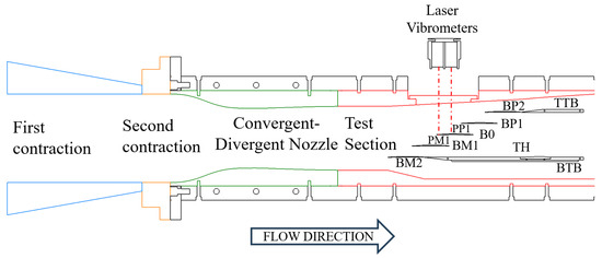
Figure 1.
TLC cross-section at 50% span.
2.2. Experimental Setup
The experimental approach is divided into two sections: steady-state and aeroelastic responses. A steady-state operational point is mapped in regions upstream of the blades, at the passage, and downstream of the blades. Figure 2 displays key location points where different methods are implemented. Red circle markers represent pressure taps located a quarter chord upstream from the blades along the pitch direction. Blue squares show pressure taps located half a chord downstream of the blade trailing edge. Circle and square markers are referred to as upstream and downstream locations, respectively. The velocity and flow angle are measured between the inlet (green triangles) and the upstream regions, as well as in both adjacent passages to B0 via a non-intrusive Laser-2-Focus (L2F) anemometer consisting of 570 measurement locations, at a operating point. The blade loading is mapped by swapping a set of blades with 15 pressure taps each, located at an 85% span. The closest tap to the leading edge on the suction side is located at a 13.6% chord due to manufacturing constraints. This location is downstream of the shock location and the separated bubble, with no direct measurements produced at these locations. A flow visualization technique was applied on the blades to confirm a separation bubble and to quantify its reattachment length. This method consists of a mix of pigment powder and a silicon-based oil, Rhodorsil 47-V1000, with a ratio of approximately 1 mL to 0.3 g. It was observed that the ratio depended on the location of the paint and the operational point. Further details regarding instrumentation and operating points can be found in Tavera Guerrero et al. [16,17].
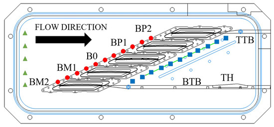
Figure 2.
Test section measurement regions. Inlet (green triangles), upstream (red circles), and downstream (blue squares) locations.
Aeroelastic measurements are performed by imposing a frequency-controlled oscillation to the central blade (B0), referred to as an oscillating blade that is either instrumented on the PS or SS. An oscillating blade is instrumented with a set of two piezo-electric actuators (MFC P1 type—M-2814-P1). An elastic filler is applied over the piezo-actuators to preserve its aerodynamic properties and ensure a smooth surface. A signal generator controls the excitation frequency and phase in order to match the test object eigen-frequency (), where n represents the mode number. The blade RMS displacement amplitude () is calculated via a laser vibrometer Keyence LKG-152 coupled to the data acquisition system DTS Slice Pro Slim. Multiple chord and span locations are measured to experimentally map the first seven modeshapes with similar mounting boundary conditions as in the TLC. The first and second modeshape correspond to the first flex and first torsion, respectively. Further details can be found in Glodic et al. [18]. In the TLC, the vibrometers are located at an 85% span along 4.8% and 41.4% of the chord. The elastic filler produced a decreased amplitude of the first flex mode from 1.2 mm to 0.74 mm at a 4.8% chord location. A decrease in vibration amplitude is accepted as a trade-off in order to not jeopardize the aerodynamic geometry and the modeshape is assumed to not be affected.
The unsteady pressure is quantified by a set of miniature surface-mounted pressure transducers, Kulite LQ-160, located at 85% span. An absolute pressure steady calibration is performed on all transducers. Each oscillating blade has eight transducers either on the PS or SS, due to geometry constraints. Each transducer is back-mounted into the blades in a representative flush-mounted configuration, as shown in Figure 3, to not influence the aerodynamic airfoil characteristics. A small volume, ≈13.3 mm3, exists between the pressure tap and the Kulite membrane. Dynamic calibration is performed due to the existing volume of air, but negligible pressure damping and phase shift are found for the frequency range of interest, up to 500 Hz.
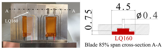
Figure 3.
Back-mounted LQ-160 Kulites in an oscillating blade. Dimensions in millimeters.
Multiple experiments are performed to ensure that the instrumented oscillating blade has a minimum electromagnetic influence, which is tested up to 3 kHz. The unsteady pressure of the two adjacent passages from B0 is reconstructed by switching instrumented blades, producing two independent experiments in the passages of interest. These locations are of relevance because the unsteady pressure is the highest due to the oscillating blade. Unsteady data are recorded after achieving a steady-state operating point. At each experiment, a frequency sweep is performed to identify the structural resonance of the oscillating blade. For each excitation frequency, multiple recording time lengths are assessed to guarantee statistically independent results, resulting in a 5 s acquisition time at a sampling frequency of 20 kHz. Each Kulite unsteady pressure is assumed to be fully independent from one another leading to a linear single-input single-output (SISO) system. Figure 4 displays a characteristic system between the blade vibration and a transducer, where capital letters represent the frequency domain. The supply voltage V is controlled, whereas the flow F produces pressure fluctuations inherent to the flow field. These produce a blade vibration X response that is measured and subjected to a noise N. The blade vibration is the input of a measured unsteady pressure response P subjected to a noise M from the data acquisition system when it excites the pressure transducers.
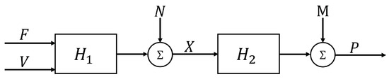
Figure 4.
Single-input–single-output system characterization.
The unsteady pressure and B0 amplitude at the first eigen-frequency () are obtained by the Welch method, performing a Hanning-windowed overlapped averaged power-spectral density (PSD) based on Equation (1), as described by Solomon [19].
Here, denotes the input signal, the Hanning window signal, and and are amplitude correction factors for the Hanning window and noise band correction, respectively. The Welch method was used with 4096 FFT points with a 50% overlap, generating a frequency resolution of Hz. This method shows a higher degree of consistency in computing RMS amplitudes when the recorded signal contains broad bandwidth content. In this case, a standard FFT predicts amplitude fluctuations from experiment to experiment due to signal leakage. The post-processing methodology starts by removing low-pass filters and zero offsets from the data acquisition system to collect the raw signal. A steady-state calibration is applied to the Kulite transducers. An FFT identifies the actual excitation frequency (). Afterward, the PSD is calculated, and the PSD is integrated around .
A correction of an induced unsteady pressure due to the transducer membrane acceleration was performed in an in-house vacuum chamber, , as shown in Figure 5. The induced pressure was measured at the experimental vibration amplitude in the flow and mapped by the vibrometers at the same location as in the TLC. The corrected magnitudes are in the order of 50 Pa.
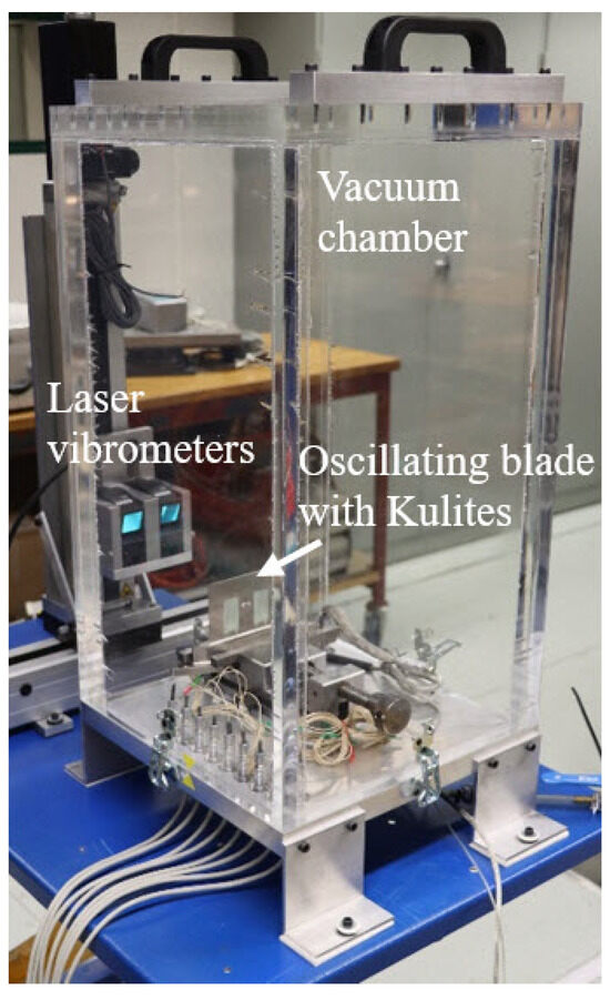
Figure 5.
Vacuum chamber for Kulite-induced pressure calibration.
The phase lag between B0 displacement and the unsteady pressure was calculated using two methods for post-processing validating purposes. The first is in the frequency domain, where an FFT at both signals is performed, and the phase difference between signals is calculated at the excitation frequency. The second is in the time domain using a cross-correlation function of both signals and computing the time lag where the signals have the highest correlation. This fraction of the time lag with respect to the oscillating period allows a phase angle calculation for unit consistency between methods. Both methods show similar phase lags with an average difference of ≈0.6°, gaining confidence in the processing method. The phase calculation using FFT is the selected method due to its fast computation compared to a cross-correlation.
Attempts to evaluate the aeroelastic response at the second mode (1st torsion) were made. However, the mode showed strong aerodynamic damping, leading to a frequency response function where no structural resonance peak was observed. It is assumed that non-linear mechanisms at the fixing hub might dominate the response. Thus, this paper presents only the results of the 1st flex. The first mode has a reduced frequency of 0.69 based on the blade chord. The piezo-electric actuator is excited from 1200 V to −500 V. Several tests were performed to identify if the asymmetric excitation would affect the test case response. It is observed that the harmonic blade response is symmetric, producing higher vibration amplitudes, and is not affected by an asymmetric input.
2.3. Numerical Setup
Due to instrumentation and inflow mass flow constraints, emphasis was placed on reproducing the whole experimental test rig setup in the numerical domain. The TLC was meshed in ICEM CFD. Figure 6 displays the domains for numerical analysis. The mesh consists of ≈12.8 million elements according to a mesh independence study. The test section contains ≈95% of the total elements. The test section has two high-refinement regions, the first of which is near the LE of each blade to capture the separation bubble. The second is along the blade tip in the spanwise direction to capture the tip gap effect over the plane of interest. The blades, including the tip, have a maximum . Steady and unsteady numerical results are obtained by an Ansys CFX solver with an SST turbulence model with a reattachment modification (RM) [20]. This turbulence modification showed a similar qualitative agreement to SST with a turbulence transition for induced separation , without solving two additional transport equations. Further details can be found in Tavera Guerrero et al. [16]. The inlet boundary conditions are imposed at the first contraction, where the stagnation chamber is located, and experimental total pressure and total temperature are measured. The outlet boundary condition is controlled by a total-to-static pressure ratio, where a static pressure at the test section outlet is imposed. Steady-state flow properties such as Mach number, pressure, and total pressure showed fluctuations of 0.6% where convergence is assumed at upstream and downstream locations at an 85% span.

Figure 6.
Numerical domain of the transonic linear cascade.
The modeshapes are computed through Ansys Mechanical, where a fixed boundary condition is imposed on the blade root. The left side of Figure 7 presents the projected first flex onto the CFD B0 mesh, and the right side is the mapped experimental modeshape. There is a qualitative agreement where the highest displacement is observed at the LE tip with an amplitude gradient towards the trailing edge. At the top of the figure, the reference airfoil at an 85% span is shown with its representative maximum and minimum displacements from the first mode. The displacement in the bending direction is approximately two orders of magnitude larger than the other directions, indicating that this mode is representative of a first flex. The modeshape was scaled to match the experimental vibration amplitude ( = 0.14 mm) with the experimental eigen-frequency ( Hz). The time step was chosen to be a 40th of the oscillation period () for an accurate amplitude resolution. Convergence is assumed when the properties of interest display less than 1% variation in mean and harmonic amplitudes of at least the last two periods. Some of the main properties of interest are the blade loading and pressure monitor points at the same locations as the experimental configuration. Finally, the time history of the unsteady pressure and blade motion is processed via an FFT.
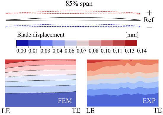
Figure 7.
Numerical and experimental qualitative comparison of the first flex.
3. Results and Discussion
3.1. Steady-State Aerodynamics
The numerical Mach number field at 85% is displayed for both operating points in Figure 8. The zero coordinate represents the rotation axis at B0. The x-axis is normalized by the chord while the y-axis displays the test section height. The axes do not have the same scale for better visualization. This figure displays local flow features upstream, at the blade passages, and downstream of the test section. The supersonic pockets are localized at the leading edge for both operating points. These regions are small, with respect to the chord, and downstream, it is assumed that the flow reattaches. At both operating points, the supersonic pocket size increases towards BP1. This local acceleration is associated with the end-wall interaction with BP2. At , a key difference occurs at the passages of interest (PM1 and PP1). The low-momentum regions appear to be influenced by the separated flow along BM2 SS, which might be driven by the bottom bypass. At the upstream location between the passages of interest, the numerical results predict an incidence angle of and at and , respectively.
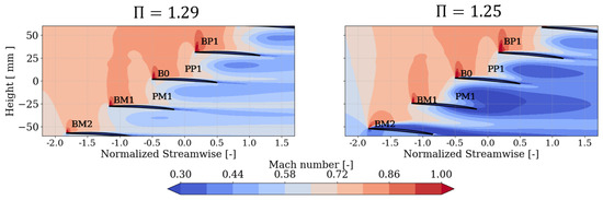
Figure 8.
Numerical Mach number comparison at 85% span for and .
At , experimental data were measured to identify numerical discrepancies. The mapped regions are upstream of the blades, and at the adjacent passages of B0, they are up to 1.5 mm away from the blade surface due to reflections. The velocity field is measured by an L2F anemometer, while the Mach number is calculated by assuming a calorically perfect gas. Under this assumption, the static temperature T is computed from the total enthalpy definition, Equation (2), as the total temperature = 303 K ± 0.5 K is measured at the stagnation chamber. Finally, the Mach number is calculated by the ratio of velocity and local speed of sound. The measured upstream average incidence angle by L2F is , displaying a difference between numerical and experimental data with a qualitative agreement.
Figure 9 shows the experimental and numerical Mach number comparison at . The upstream region displays an acceleration trend towards the BP1 index that is captured by both methods, leading to a stronger supersonic pocket in B0 compared to BM1, inferring that the local flow features can differ between those blades. L2F data show that the flow is subsonic downstream of the supersonic pocket due to the presence of a shock wave, indicating that the flow had reattached. These supersonic pocket regions are in agreement between the two methods. At the adjacent passages from B0, both cases predict that PM1 contains a wider low-momentum region associated with higher losses that are dominated by three-dimensional effects. As the measurement plane is 85% of the span, it is assumed that the tip leakage vortex is the main driver of losses. CFD displays a qualitative agreement with experimental data, but quantitative differences are observed in low-momentum regions, potentially driven by the bottom bypass blockage.
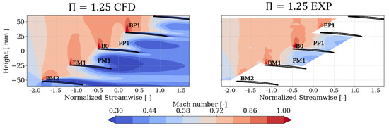
Figure 9.
Experimental and numerical Mach number comparison at 85% span for .
Under a calorically perfect fluid assumption, the isentropic Mach number is calculated from the isentropic flow relationships, Equation (3), with a constant specific heat ratio . The total reference pressure is measured at the stagnation chamber. Figure 10 displays the experimental and numerical isentropic Mach number () for both operating points. This figure represents data from the upstream and downstream locations in red and blue, respectively. Experimental and numerical data are denoted by markers and lines, respectively. PM1 and PP1 are represented with colored backgrounds for spatial localization purposes with respect to the normalized pitch. The experimental data error bars correspond to a 95% confidence interval over ≈15 min. At both operating points, the acceleration gradient towards BP1 is observed as well as the local acceleration regions due to the supersonic pocket. The upstream and downstream CFD trends are in good agreement with the experimental data. The strongest discrepancy is observed at NS between −1.5 and −1.0 normalized pitch, where the BM2 separation might be over-estimated by CFD.
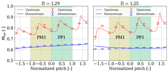
Figure 10.
Experimental and numerical upstream and downstream location comparisons at and at 85% span.
The steady-state blade loading is measured by swapping the different instrumented blades, producing three independent experiments. Figure 11 shows, in the y-axis, the isentropic Mach number of the experimental data (markers) and CFD (lines) along the normalized chord in the x-axis. At both operating points, the blade loading results do not show a pressure plateau due to the separation region, inferring that the separation is small and local. At , B0 and BM1 show differences in incidence angle as BM1 has a higher front-loaded characteristic. It is observed that the pressure sides are distinct from one another, but the numerical setup can capture this trend. Similarly, CFD predicts that within the first 15% chord, the shock-induced separation mechanism acts similarly among the blades, assuming a similar reattachment length. The first pressure tap along SS at both operating points shows that CFD overpredicts the pressure recovery gradient where the highest discrepancies are observed. At , numerical results show a qualitative difference at BM1, predicting a lower incidence angle with respect to the other blades, indicating a smaller supersonic pocket and smaller reattachment length. It is assumed that this qualitative difference might arise from the interaction between the bottom bypass and the separated flow from BM2 SS. In both cases, both experimental and numerical results show that the flow-field characteristics of the adjacent passages from B0 are slightly different, with the highest differences observed on the pressure side. The numerical results are able to predict the experimental data with good qualitative agreement, except at the first pressure tap.
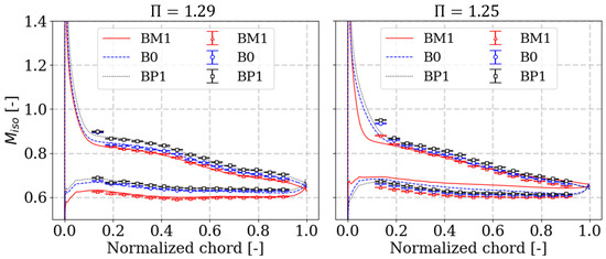
Figure 11.
Experimental and numerical blade loading comparisons at and at 85% span.
Flow visualizations are performed at the suction side of BM1, B0, and BP1, confirming a separation bubble near the leading edge. A ramp-up to the desired operating points takes ≈50 s due to facility capabilities. After the operating point is set, the flow conditions are kept for ≈10 min for the pigment to dry. When ramping down, transient effects can potentially affect the predicted separation bubbles depending on the paint placement. An iterative procedure showed that the paint should be placed in the nearby region of the separation line and close to the leading edge to trace the separation line. The streamlines show a spanwise component, shifting the excess of paint toward the mid chord. Care was focused on applying enough paint to visualize the bubble while minimizing the concentrated paint moving downstream when ramping down. The experimental reattachment line is measured digitally by a pixel-to-mm correlation and compared to a physical known measurement, showing ±0.2 mm fluctuations. Numerical results are computed from the two nodes, along the chord, at which the shear stress changes its sign. It is assumed that there is a linear shear variation between these points, where a line equation is calculated, as well as its shear zero intersection. This method minimizes the influence of mesh spatial resolution over the calculated reattachment line length. Figure 12 displays B0 surface streamlines of both operating points with the same zoom-in area towards the leading edge tip. In this region, a reattachment line is observed (orange line). Three-dimensional effects are observed at the blade tip, up to an ≈80% span, leading to reattachment length fluctuations within this region.
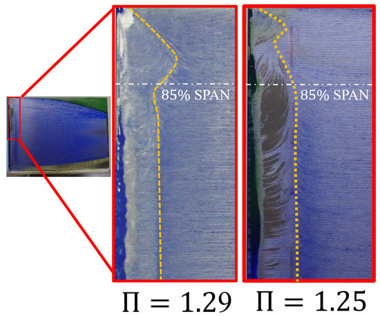
Figure 12.
B0 reattachment line at and .
At the reference span, qualitative differences among blades and numerical predictions were observed. Table 2 summarizes the predicted reattachment length for both methods at 50% to avoid three-dimensional influence for comparative purposes. At , where a higher incidence angle takes place, the reattachment line is further downstream for each blade compared to . These results are consistent with a shock-induced separation mechanism. Numerical predictions have a standard deviation of 0.7 mm with respect to experimental data. The differences in reattachment length among the blades are attributed to the observed different inlet upstream isentropic Mach numbers. BM1 shows the maximum deviation, 1 mm, at both operating points, which is assumed to occur due to BM2 interaction. These results are in agreement with the qualitative differences observed at BM1 blade loading at .
Table 2.
Experimental and numerical reattachment line length at 50% span at and .
3.2. Aeroelastic Response
The eigen-frequency of the first flex mode () is compared for two configurations, with and without flow, as shown in Table 3. The experimental blade vibration and unsteady pressure from the representative flush-mounted transducers are measured by a frequency sweep; at each excitation frequency, a measurement is taken. For both with-/without-flow configurations, a resonance peak is measured experimentally. At the operating points, the oscillating blade is subjected to a static deformation of around 1.9 mm. This steady-state pre-stress produces an increase in the blade stiffness leading to a shift in the natural frequency of 2 Hz. Laser vibrometer data at two different locations showed an in-phase motion, and thus the modeshape is assumed to not be modified. The most significant difference lies in the vibration amplitude showing that with the flow, the amplitude is damped by ≈5.7 times due to the aerodynamic damping.
Table 3.
Modal property comparisons with and without flow.
An analysis of the first system is performed for two configurations when the voltage (V) is either active or not, where the blade vibration is measured for both configurations. By performing a PSD over B0 at these configurations, it is possible to have an insight into which mode dominates and, by extension, an idea of the energy content of the flow. It is assumed that the flow inside the TLC presents a random nature, similar to a broad bandwidth excitation source. The PSD of the blade for both configurations is shown in Figure 13. When there is no controlled oscillation (voltage OFF), the first three modes contain a similar contribution to the blade motion with a slight dominance of mode 1. This observation suggests that the inherent energy content of the flow is indeed a broad bandwidth case. When the first mode is excited (voltage ON), mode 1 response increases by almost four orders of magnitude, and it is higher than the other modes by two orders of magnitude. These measurements infer that a single-mode excitation assumption is valid.
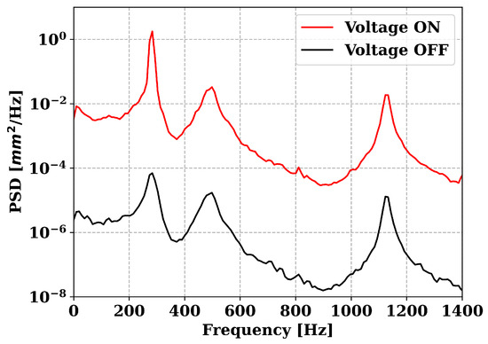
Figure 13.
B0 PSD difference with and without input voltage excitation.
B0 harmonic pressure magnitudes are corrected by a vacuum unsteady pressure, . The modulus of the harmonic unsteady pressure coefficient, , is defined in Equation (4), where the corrected harmonic pressure is normalized by the vibration amplitude, , with a reference pressure being the dynamic head between the total pressure and the static isentropic pressure for Mach 0.81, and the chord .
Figure 14 shows the distribution of the unsteady pressure coefficient amplitude, , in the TLC over a period. The reference plane is 85%, and the operating point is . The black arrows point out the location of each blade near its leading edge, where the shock-induced mechanism takes place. The maximum amplitude is observed in the oscillating blade with a clear decay at BP1 and BM1. In the oscillating blade, the unsteadiness combines the blade motion, the leading edge high-pressure gradient, and the shock. This suggests that the pressure field of these components will dominate the harmonic amplitudes on the suction side. The unsteady pressure propagates upstream and downstream of the cascade with no apparent reflection from the surrounding walls.
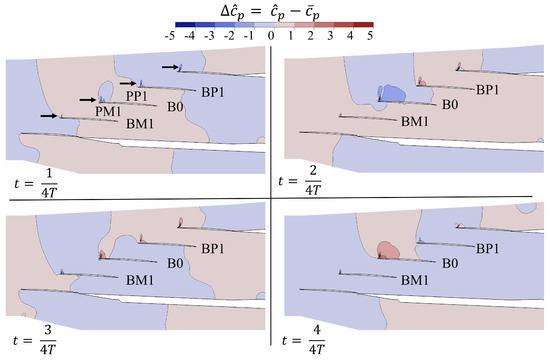
Figure 14.
Numerical unsteady pressure coefficient, , and its distribution over a period at 85% span for .
Figure 15 displays the experimental (markers) and numerical (lines) unsteady pressure coefficient amplitude, , against the normalized chord at 85% and 50% spans. Numerically, the reattachment length is denoted by a shaded background, and its normal shock location is denoted by a diamond marker on B0. For all cases, the highest amplitude is observed on B0 near the leading edge on the suction side. The adjacent blades show a clear amplitude decay with respect to the oscillating blade. From steady-state blade loading, there is no clear indication that the small separation bubble affects the pressure field. Figure 14 also shows that the unsteady pressure field is dominated by the large pressure gradient near the blade’s LE. At an 85% span in both operating points, it is shown that the highest harmonic amplitude occurs at the shock location with no direct correlation between and at the reattachment line. The first two Kulites are located at 13% and 24% chords, limiting a direct measurement in the separated area and the shock. At the first Kulite, both methods agree in amplitude while the harmonic amplitude decays at , possibly from the near-wall effects as shown by flow visualizations. However, between the first and second Kulite, the experimental B0 SS response shows a fast decrease in that is not observed numerically. At both operating points, downstream of the second Kulite, an ≈30% chord, the amplitudes are of the same order as , but this trend is not observed numerically. Numerically, there is a smooth amplitude decrease towards the trailing edge, highlighting a clear qualitative difference between methods at B0. The numerical amplitudes at a 50% span are included to isolate three-dimensional effects that might occur on the suction side aft region. However, the smooth decay towards the trailing edge is also present at both operating points. It is also observed that the shock location no longer matches the maximum response amplitude. The presented numerical trends agree with Wantanabe and Aotsuka [10] for at different incidence angles, where the turbulence model has been used. This indicates that a qualitative agreement might be possible without a refined mesh . However, based on the experimental data, it is hypothesized that CFD overpredicts the response downstream of the shock wave, but more experimental data at different spans are required to falsify or support this statement. Due to the challenging flow features, the usage of local point-wise measurements shows its limitations. On the other hand, these results indicate that there is an agreement between the numerical and experimental data at the adjacent passages (BM1 SS and BP1 PS) from B0 at both operating points. Experimental confirmation at different spans would be required to gain a higher degree of confidence in the numerical predictions. This can be explored in future work, as it could not be presented here due to instrumentation limitations.
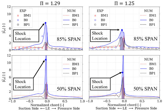
Figure 15.
Aeroelastic response amplitude vs. normalized chord at 50% and 85% spans for and . Numerical reattachment locations (colored background). Numerical shock location (blue diamond).
Figure 16 shows the comparison between experimental and numerical local phase angles at an 85% span for both operating points. The phases from B0 were calculated before correcting by the induced pressure in vacuum to enhance the signal quality. At BM1 and B0, there is a qualitative agreement on the suction side with similar trends at both operating points. On the pressure side, B0 shows a qualitative agreement with the numerical trend prediction but shifted by , with no clear root cause. The highest qualitative difference takes place on the pressure side of BP1. It is acknowledged that some level of uncertainty might come from a low signal amplitude. However, this post-processing method has shown a good quantitative agreement at high reduced frequencies, as shown in Glodic et al. [21].
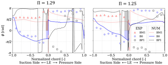
Figure 16.
Aeroelastic response phase vs. normalized chord at 85% span for and .
Figure 17 shows the unsteady pressure coefficient distribution on B0 SS at 85% and 50% for both operating points. At each span, a small normal plane adjacent to the blade covers 20% of the chord where the supersonic pocket (green), separation, and reattachment lines (yellow) are highlighted. It is observed that there is a correct prediction of an increase in supersonic pocket size at , as the incidence angle increases. In both operating points at 85% span, it is clear that the supersonic pocket size and unsteady pressure amplitude are reduced with respect to 50% span. However, shows a stronger unsteady pressure where the supersonic shock ends, while shows a lower unsteady pressure. This indicates that in the measurement plane, at , the unsteady pressure amplitude is driven by a combination of the shock and near-wall effects, with no direct correlation to the separated area. Downstream of the blade at 85% span, there is a smooth decrease in amplitude towards the trailing edge without a clear driving mechanism that could explain the amplitude overprediction with respect to experimental data. At a 50% span of both operating points, the perpendicular plane shows that the highest unsteady pressure amplitude occurs at the end of the supersonic pocket, which finishes with a shock wave, with a clear phase shift. It is also shown that on B0 SS, from the leading edge towards the separation line, there is an amplitude increase. This interaction is assumed to come from the large pressure gradient due to the high incidence.
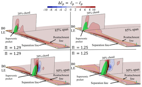
Figure 17.
Numerical unsteady pressure coefficient, , at B0 at a time step at 50% and 85% spans with a zoom-in of the shock-induced separation mechanism for and .
Figure 18 displays the distribution of the harmonic pressure coefficient amplitude, , on the central blade suction side up to 50% chord for both operating points. The figure shows the separation onset as a dashed white line, the reattachment line in dotted black, and the shock location in magenta, along with three different spans for spatial location purposes. In the midspan region, the maximum harmonic amplitude is located at the separation onset and not directly under the shock. Figure 17 shows that the shock is the main driver for the harmonic response that appears to be impinging on the separation line. At , this interaction is stronger as the supersonic pocket is smaller and closer to the separation line. On the other hand, at , the shock is larger and further downstream from the separation line, showing a lower amplitude downstream of the separation line. In either case, the reattachment line does not show an influence on the harmonic amplitude. Towards the tip, at 85% and 95% spans, the harmonic amplitude is affected by near-wall effects and tip leakage. In these regions, the largest harmonic magnitude is not at the separation onset but at the shock location, as shown before in Figure 15. At the measurement span, it is shown that downstream of the reattachment line, there is no mechanism that can explain the CFD overprediction with respect to the experiments. Further experimental campaigns at several spans can help to bring clarity for validation purposes; however, due to experimental instrumentation constraints, this could not be performed in the current study, but it should be studied in future research.
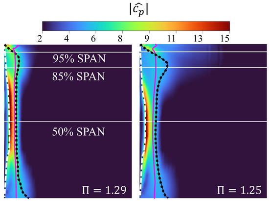
Figure 18.
Distribution of the aeroelastic response amplitude on the central blade suction size up to 50% chord. Separation line (white dashed line), reattachment line (dotted black line), and shock location (continuous magenta line).
4. Conclusions
The numerical and experimental aeroelastic response of the first flex modeshape was compared at the oscillating transonic linear compressor cascade. Focus was placed on reproducing the whole experimental test rig to compare experimental data at two operating points. The operating points, and , represent a transonic compressor’s peak efficiency and near stall at part speed, respectively.
The main outcomes are summarized as follows:
- The central (B0) and adjacent blades (BP1 and BM1) are subjected to slightly different upstream conditions that modify the blade loadings at each operating point. However, the numerical model can predict such differences with a quantitative agreement.
- A small separation bubble was confirmed experimentally. At an 85% span, near-wall effects are visible, and reattachment length measurements are carried out at 50% to avoid three-dimensional influence. The numerical reattachment length is within a 0.7 mm standard deviation from experimental data for both operating points.
- At both operating points, the numerical harmonic pressure amplitude coefficient at midspan shows that the shock is the main contributor. The shock interacts with the separation onset, where its maximum amplitude is located. The amplitude from this interaction decreases between and , as the shock location is further downstream from the separation line at .
- At both operating points, the numerical harmonic pressure amplitude is affected by near-wall effects. At the measurement plane, the shock dominates the response with an agreement between the maximum amplitude and the shock location.
- Experimental and numerical data at an 85% span display a qualitative agreement in the harmonic pressure at the adjacent blades BM1 and BP1. However, on the suction side of the oscillating blade, there is a qualitative difference between both methods downstream from an ≈30% chord, where CFD appears to be overpredicting the harmonic amplitude with no clear root cause. The phase showed larger qualitative variations on the Blade Plus 1 pressure side, which was attributed to a low signal amplitude.
Author Contributions
Conceptualization, N.G. and H.M.; methodology, C.A.T.G., N.G. and M.G.S.; software, C.A.T.G. and M.G.S.; validation, C.A.T.G., N.G. and M.G.S.; formal analysis, C.A.T.G. and N.G.; investigation, C.A.T.G. and N.G.; resources, N.G. and M.G.S.; data curation, C.A.T.G.; writing—original draft preparation, C.A.T.G.; writing—review and editing, N.G., M.G.S. and H.M.; visualization, C.A.T.G.; supervision, N.G. and M.G.S.; project administration, N.G.; funding acquisition, N.G. and H.M. All authors have read and agreed to the published version of the manuscript.
Funding
This research was funded by VINNOVA (Swedish Agency for Innovation Systems), grant number 2019-02748. The APC was also funded by the same VINNOVA grant.
Institutional Review Board Statement
Not applicable.
Informed Consent Statement
Not applicable.
Data Availability Statement
Data are fully available for sharing upon direct request to the main author of this paper.
Acknowledgments
The authors highly appreciate the work carried out by KTH technicians Emil Lindström and Leif Petterson. Without their support and input, these experimental studies would have not been possible.
Conflicts of Interest
Author Hans Mårtensson was employed by the company GKN Aerospace Engines. The remaining authors declare that the research was conducted in the absence of any commercial or financial relationships that could be construed as a potential conflict of interest.
Nomenclature
The following nomenclature is used in this manuscript:
| Abbreviations | |
| A | Amplitude of vibration |
| BM1 | Blade Minus 1 |
| BM2 | Blade Minus 2 |
| BP1 | Blade Plus 1 |
| BP2 | Blade Plus 2 |
| B0 | Blade Zero |
| LE | Leading edge |
| PS | Pressure side |
| PSD | Power-spectral density |
| RM | Reattachment modification |
| PM1 | Passage Minus 1 |
| PP1 | Passage Plus 1 |
| SS | Suction side |
| TE | Trailing edge |
| TLC | Transonic linear cascade |
| VINK | Virtual Integrated Compressor |
| Subscripts | |
| iso | Isentropic |
| ref | Reference value |
| rms | Root-mean-squared |
| tot | Total flow property at stagnation chamber |
| 0 | Total local flow property |
| vacuum | Vacuum conditions |
| Latin | |
| M | Mach number |
| Complex unsteady pressure coefficient | |
| P | Pressure |
| T | Temperature |
| V | Voltage |
| Geek | |
| Total-to-static pressure ratio | |
| Eigen-frequency | |
| Phase lag between blade motion and pressure |
References
- Biollo, R.; Benini, E. Recent advances in transonic axial compressor aerodynamics. Prog. Aerosp. Sci. 2013, 56, 1–18. [Google Scholar] [CrossRef]
- Thermann, H.; Niehuis, R. Unsteady Navier-Stokes Simulation of a Transonic Flutter Cascade Near-Stall Conditions Applying Algebraic Transition Models. J. Turbomach. 2005, 128, 474–483. [Google Scholar] [CrossRef]
- Srinivasan, A.V. Flutter and Resonant Vibration Characteristics of Engine Blades. J. Eng. Gas Turbines Power 1997, 119, 742–775. [Google Scholar] [CrossRef]
- Holzinger, F.; Wartzek, F.; Schiffer, H.P.; Leichtfuss, S.; Nestle, M. Self-Excited Blade Vibration Experimentally Investigated in Transonic Compressors: Acoustic Resonance. J. Turbomach. 2015, 138, 041001. [Google Scholar] [CrossRef]
- Bölcs, A.; Fransson, T.H. Aeroelasticity in Turbomachines. Comparison of Theoretical and Experimental Cascade Results; Technical Report; Ecole Polytechnique Federale de Lausanne (Switzerland) lab de Thermique: Lausanne, Switzerland, 1986. [Google Scholar]
- Hanamura, Y.; Tanaka, H.; Yamaguchi, K. A Simplified Method to Measure Unsteady Forces Acting on the Vibrating Blades in Cascade. Bull. JSME 1980, 23, 880–887. [Google Scholar] [CrossRef]
- Ellenberger, K.; Gallus, H.E. Experimental Investigations of Stall Flutter in a Transonic Cascade. In Turbo Expo: Power for Land, Sea, and Air; American Society of Mechanical Engineers: New York, NY, USA, 1999; p. V004T03A047. [Google Scholar] [CrossRef]
- Buffum, D.H.; Capece, V.R.; King, A.J.; EL-Aini, Y.M. Oscillating Cascade Aerodynamics at Large Mean Incidence. J. Turbomach. 1998, 120, 122–130. [Google Scholar] [CrossRef]
- Yang, H.; He, L. Experimental Study on Linear Compressor Cascade with Three-Dimensional Blade Oscillation. J. Propuls. Power 2004, 20, 180–188. [Google Scholar] [CrossRef]
- Watanabe, T.; Aotsuka, M. Unsteady Aerodynamic Characteristics of Oscillating Cascade With Separation Bubble in High Subsonic Flow. In Volume 4: Turbo Expo 2005; American Society of Mechanical Engineers: New York, NY, USA, 2005; pp. 625–633. [Google Scholar] [CrossRef]
- Vogt, D.; Fransson, T. A Technique for Using Recessed-Mounted Pressure Transducers to Measure Unsteady Pressure. In Proceedings of the 17th Symposium on Measuring Techniques in Transonic and Supersonic Flows in Cascades and Turbo machines, Stockholm, Sweden, 9–10 September 2004. [Google Scholar]
- Lepicovsky, J.; McFarland, E.; Capece, V.; Jett, T.; Senyitko, R. Methodology of Blade Unsteady Pressure Measurement in the NASA Transonic Flutter Cascade; Technical Report No. NASA/TM-2002-211894; NASA Center for Aerospace Information: Hanover, MD, USA, 2002.
- Fransson, T.H.; Jöcker, M.; Bölcs, A.; Ott, P. Viscous and Inviscid Linear/Nonlinear Calculations Versus Quasi-Three-Dimensional Experimental Cascade Data for a New Aeroelastic Turbine Standard Configuration. J. Turbomach. 1999, 121, 717–725. [Google Scholar] [CrossRef]
- Lejon, M.; Grönstedt, T.; Glodic, N.; Petrie-Repar, P.; Genrup, M.; Mann, A. Multidisciplinary Design of a Three Stage High Speed Booster. In Turbo Expo: Power for Land, Sea, and Air. Volume 2B: Turbomachinery; American Society of Mechanical Engineers: New York, NY, USA, 2017; p. V02BT41A037. [Google Scholar] [CrossRef]
- Tian, S.; Petrie-Repar, P.; Glodic, N.; Sun, T. CFD-Aided Design of a Transonic Aeroelastic Compressor Rig. J. Turbomach. 2019, 141, 101003. [Google Scholar] [CrossRef]
- Tavera Guerrero, C.; Glodic, N.; Groth, P. Validation of Steady-State Aerodynamics in a Transonic Linear Cascade at Near Stall Conditions. In Turbo Expo: Power for Land, Sea, and Air. Volume 10A: Turbomachinery—Axial Flow Fan and Compressor Aerodynamics; American Society of Mechanical Engineers: New York, NY, USA, 2022; p. V10AT29A013. [Google Scholar] [CrossRef]
- Tavera Guerrero, C.; Glodic, N.; Mårtensson, H. Steady-state aerodynamics tip gap influence in a transonic linear cascade at near stall. In Proceedings of the International Council of the Aeronautical Sciences (ICAS), Stockholm, Sweden, 4–9 September 2022. [Google Scholar]
- Glodic, N.; Guerrero, C.T.; Salas, M.G. Blade oscillation mechanism for aerodynamic damping measurements at high reduced frequencies. E3S Web Conf. 2022, 345, 03002. [Google Scholar]
- Solomon, O.M., Jr. PSD Computations Using Welch’s Method. [Power Spectral Density (PSD)]; USDOE: Washington, DC, USA, 1991. [CrossRef]
- Ansys. CFX-Solver Solver Theory Guide Section: 2.2.2.4.4; R2; Ansys: Canonsburg, PA, USA, 2021. [Google Scholar]
- Glodic, N.; Tavera Guerrero, C.; Gutierrez, M. Aeroelastic Response of a Transonic Compressor Cascade at High Reduced Fequencies. In Proceedings of the ISUAAAT16, Toledo, Spain, 19–23 September 2022. [Google Scholar]
Disclaimer/Publisher’s Note: The statements, opinions and data contained in all publications are solely those of the individual author(s) and contributor(s) and not of MDPI and/or the editor(s). MDPI and/or the editor(s) disclaim responsibility for any injury to people or property resulting from any ideas, methods, instructions or products referred to in the content. |
© 2025 by the authors. Published by MDPI on behalf of the EUROTURBO. Licensee MDPI, Basel, Switzerland. This article is an open access article distributed under the terms and conditions of the Creative Commons Attribution (CC BY-NC-ND) license (https://creativecommons.org/licenses/by-nc-nd/4.0/).