Preliminary Assessment of Geometric Variability Effects Through a Viscous Through-Flow Model Applied to Modern Axial-Flow Compressor Blades ^†

Abstract

An important question for turbomachine designers is how to deal with blade and flowpath geometric variabilities stemming from the manufacturing process or erosion during the component lifetime. The challenge consists of identifying where stringent manufacturing tolerances are absolutely necessary and where looser tolerances can be used as some geometric variations have little or no effects on performance while others do have a significant impact. Because numerical simulations based on Reynolds-averaged Navier–Stokes (RANS) equations are computationally expensive for a stochastic analysis, an alternative approach is proposed in which these simulations are complemented by cheaper through-flow simulations to provide a finer exploration of the range of variations, in particular in the context of robust design. The overall goal of the present study is to evaluate the adequacy of a viscous time-marching through-flow solver to predict geometric variability effects on compressor performance and, in particular, to capture the main trends. Although the computational efficiency of such a low-fidelity solver is useful for parametric studies, it is known that the involved assumptions and approximations associated with the through-flow (TF) approach introduce errors in the performance prediction. Thus, we first evaluate the model with respect to its underlying assumptions and correlations. To accomplish this, TF simulations are compared to RANS simulations applied to a modern low-pressure compressor designed by Safran Aero Boosters. On the one hand, the TF simulations are fed with the exact radial distribution of the correlation parameters using RANS input data in order to isolate the modeling error from correlation empiricism. Moreover, in the context of multi-fidelity optimization, such distributions can be predicted using the more detailed RANS simulations that are performed on selected operating points. On the other hand, correlations from the literature are assessed and improved. It is shown that the solver provides realistic predictions of performance but is highly sensitive to the underlying correlations. Then, two modeling aspects linked to the blade leading edge, namely incidence correction and camber line computation, are discussed. As geometric variability precisely at the blade leading edge has a significant impact on the performance, we assess how these two aspects influence the variability propagation in this region. Moreover, we propose a strategy to mitigate these model uncertainties, and geometric variabilities are introduced at the blade leading edge in order to quantify the resulting variation in performance. Finally, within the scope of this preliminary study, perturbations of the three-dimensional position of undeformed stator blades and deformations of the hub and shroud contours are introduced one factor at a time per simulation. Their range is defined based on the tolerance limits typically imposed in the industry and on observed manufacturing variability. It is found that the through-flow model broadly provides realistic predictions of performance variations resulting from the imposed geometric variations. These results are a promising first step towards the use of the through-flow modeling approach for geometric uncertainty quantification.

1. Introduction

The axial-flow compressor design is characterized by a constant search for the best compromise between performance and manufacturing cost. The manufacturing tolerance of the blade, and in particular of its leading edge, is a good example: its shape has a high impact on aerodynamic performance whilst ensuring that the high geometric accuracy entails a severe manufacturing cost. Most modern compressor blades have traditionally been designed without considering geometric variations, although manufactured blades inevitably differ from the nominal geometry due to imperfections. Nonetheless, the impact of geometric variations can induce unacceptable performance variability and a degradation of the mean performance due to a lack of design robustness [1,2]. Owing to the increasing computational power combined with powerful new numerical techniques for optimization and uncertainty propagation, questions related to design robustness with respect to manufacturing variability can now be tackled during the design process [3]. The challenge is to find the optimal balance between performance and manufacturing cost by identifying where stringent manufacturing tolerances are absolutely necessary and where looser tolerances can be used. This can alleviate the manufacturing process and simplify the treatment of poorly constructed parts during quality control.

Recent works [4,5,6] on this topic rely on Computational Fluid Dynamics (CFD) simulations to propagate the variability in geometry to that of performance. This approach is computationally expensive as the already non-negligible cost of a single simulation, generally based on the Reynolds-averaged Navier–Stokes (RANS) equations, is further compounded by the large number of simulations required. However, it is of utmost importance to be able to predict the effects of tolerances on the performance dispersion within a time scale that is compatible with the design process. In this context, the computational efficiency of through-flow (TF) solvers is useful for parametric studies during the design improvement phases in which many parameters or geometric variabilities are involved and robust design is targeted. It is, however, known that such an averaged two-dimensional CFD modeling approach is fundamentally limited in its ability to represent turbomachinery flow features due to the intrinsic limitations of the through-flow equations and the approximations and assumptions made in the closure models [7]. It is thus unclear a priori whether the low computational cost of through-flow models can be leveraged for the practical quantification and propagation of geometric variability.

Specifically, a through-flow model, even based on Navier–Stokes (N–S) equations, cannot predict the prerotation of the flow upstream of a blade row due to the axisymmetry assumption on which the model is based [8]. In the analysis mode, the flow angles in the bladed region are imposed by a blade flow deflection force. Therefore, a discontinuity occurs at the leading edge if the flow is not aligned with the mean blade camber. This discontinuity leads to a sudden and non-physical increase in entropy and a spurious loss. A common fix consists of modifying the blade angle in the leading-edge region so that it adapts to the incident flow. As a result, the blade geometry is locally modified by this numerical artifact. Consequently, this modification will actually interfere with the correct estimation of the impact of manufacturing tolerance on the blade LE on performance.

Furthermore, modern optimized airfoils are not part of a blade family but designed to provide a certain loading distribution. Therefore, the classical camber line/thickness distribution on which TF computations rely is not readily available, nor are estimates of blade section performance. The section outline, which is split into the mean camber line and thickness distribution, must thus be obtained through an inverse computation algorithm. However, in the vicinity of the leading edge (LE) and trailing edge (TE), algorithms determining a mean camber line can be unreliable [9]. This epistemic uncertainty, although usually having a small impact, can still completely mask geometric variability in the leading edge region.

The objective of the present work is thus to evaluate the ability of the through-flow modeling approach to quantify the impact of geometric variabilities on global performance. The approach consists of a sensitivity analysis of the mass-flow rate, pressure ratio, and isentropic efficiency of a modern highly loaded multi-stage axial low-pressure compressor at nominal conditions to several types of geometric variations in the blades and endwall sections. In particular, the predictions of a tuned viscous through-flow model are compared to those of steady 3D RANS simulations. In the scope of the present work, only geometric variabilities based on the leading edge angle, the three-dimensional position of undeformed stator blades, and the deformation of the hub/shroud geometry are introduced. Each variation is considered independently of the others, one at a time. The variability range is defined based on the tolerance limits typically used in the industry.

This paper is organized as follows. First, the underlying equations of the TF solver are described, with a particular focus on the modeling aspects of its unclosed terms and correlations and the associated sources of error. The through-flow solver is also assessed based on the compressor test-case. In this context, we also propose several modifications of the correlations to improve the prediction. Then, the two modeling aspects related to the blade leading edge are discussed and strategies to mitigate these model uncertainties are proposed. Finally, geometric variations in the blade are introduced based on a simple parametrization. The results obtained with the TF model are then presented and compared to those from 3D RANS simulations. Finally, the ability of the TF model to capture the major trends and the sensitivity of the correlation outputs with respect to the geometric variabilities are discussed. The present analysis represents a first preliminary step in the overall study of geometric variabilities.

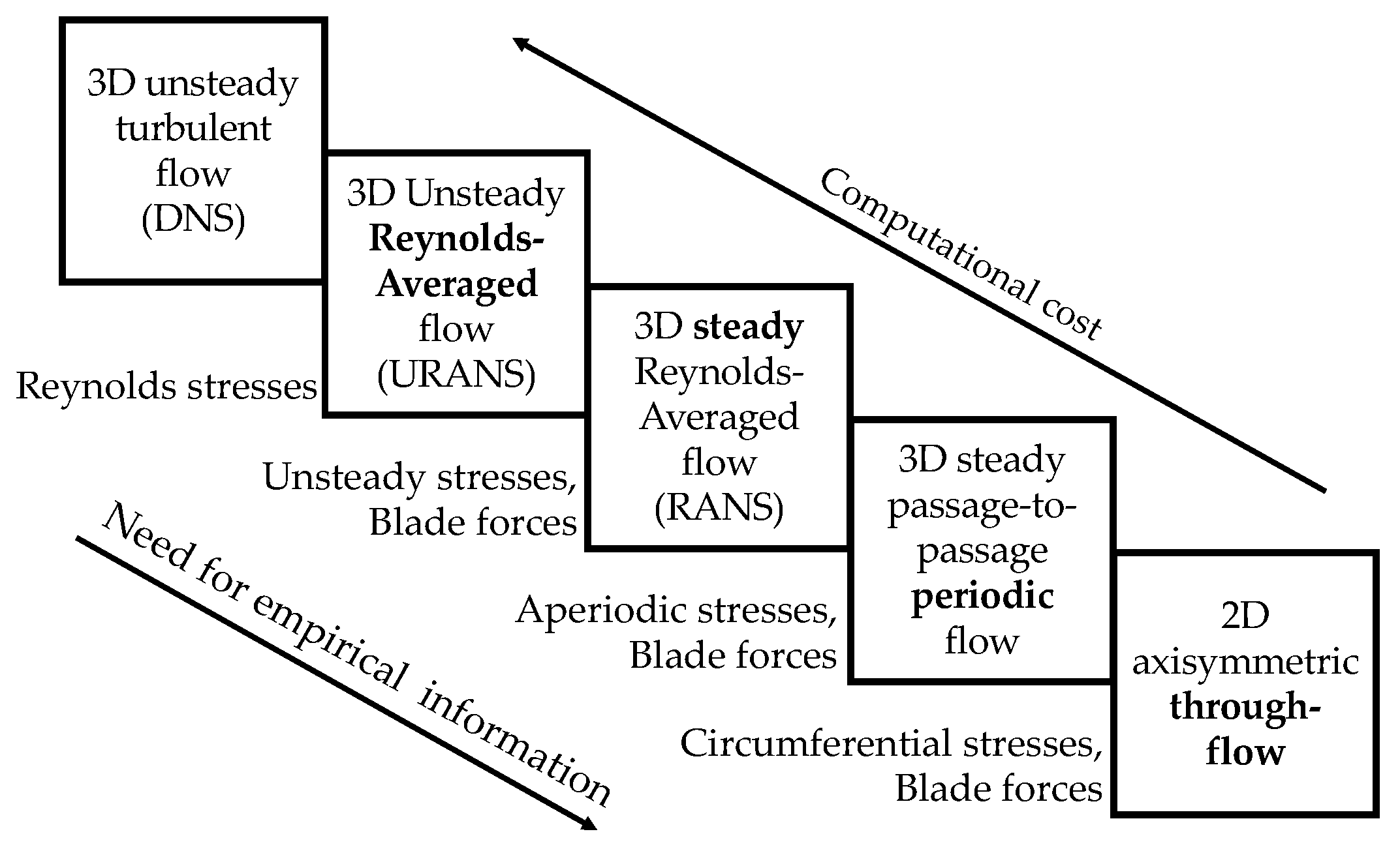
2. Through-Flow Model

The computational efficiency of through-flow methodologies stems from the pitch-wise averaged representation of the three-dimensional (3D) flow field in the meridional stream surface. However, this averaging process includes additional terms that are unclosed. Such a modeling approach has been used for decades in axial turbomachines, and many different models with various levels of approximation have been developed over the years. They can be divided into two groups. The first one is known as the streamline curvature (SLC) method [10] and remains the backbone of the industrial compressor and turbine design process. The second type of through-flow model has been driven by the growth in computing power over the years. This approach, borrowed from traditional CFD methods, is mostly based on the pitch-wise averaged inviscid Euler equations [11,12,13]. Navier–Stokes-based through-flow models, such as the one used in the present study, have also been proposed occasionally [7,14]. Because all these models are based on different governing equations and closure models, which influence the level of empiricism and error, it is important for users and developers to know the underlying assumptions in order to characterize the associated modeling error. The Adamczyk’s averaging cascade approach [7,15] formalizes the different levels of CFD modeling encountered in numerical simulations by rigorously deriving a set of equations through a cascade of averages.

2.1. Adamczyk’s Cascade

Adamczyk’s averaging cascade relies on a succession of four averages that link the three-dimensional unsteady turbulent flow to a stationary axisymmetric meridional flow, thus defining the hierarchy of modeling levels, as shown in Figure 1. Specifically, it consists of an ensemble Reynolds averaging, a time-averaging, a passage-to-passage averaging, and a circumferential averaging. The equations that are obtained for the averaged quantities are thus mathematically exact and help identifying, in a rigorous and exhaustive manner, the unclosed source terms.

These source terms can be divided into two categories. On the one hand, blade forces and blockage terms explicitly appear during the averaging process because the integration bounds of the averaging are not constant over the domain. These terms represent the forces exerted on the flow by the implicit presence of the blade in the two-dimensional meridional flow. They only apply in the region of the domain corresponding to the fictitious presence of the blade in the meridional plane. On the other hand, stresses appear due to the non-linearity of the Navier–Stokes equations. These terms represent the mean effects of the flow features that are eliminated by the averaging in the whole meridional plane. Simon [7] showed that the results of through-flow simulations fed with the exact values of source terms from corresponding high-fidelity computations lead to quasi-perfect match of performance prediction. However, these exact values are often elusive because the mathematical expressions of unclosed terms depend on quantities that are not resolved by the through-flow solver. In practice, these terms are obtained from closure models or, for some, simply neglected. These simplifications and approximations inevitably result in errors.

2.2. Viscous Through-Flow Equations

The viscous time-marching through-flow model used in the present analysis is based on the averaged Navier–Stokes equations [7]. The blade body forces are implemented in the ASTEC code developed by Safran Tech and the authors. This software is used as an add-on to the 2D version of Onera’s CFD solver elsA to provide it with the complementary source terms to ultimately solve the meridional flow. In this paper, the meridional problem is solved in the analysis mode as the performance for a known geometry is sought. The complete set of averaged equations reads in cylindrical coordinates $(x,r,\theta )$

$${\displaystyle \frac{\partial \mathbf{U}}{\partial t}}+{\displaystyle \frac{\partial \left({\mathbf{F}}_{\mathbf{i}}-{\mathbf{F}}_{\mathbf{v}}\right)}{\partial x}}+{\displaystyle \frac{\partial \left({\mathbf{G}}_{\mathbf{i}}-{\mathbf{G}}_{\mathbf{v}}\right)}{\partial r}}=\mathbf{S},$$

(1)

where x, r, $\theta$ are the stream-wise, span-wise, and pitch-wise coordinates, $\mathbf{U}$ is the vector of transported variables, ${\mathbf{F}}_{\mathbf{i}}$ and ${\mathbf{G}}_{\mathbf{i}}$ the inviscid fluxes, ${\mathbf{F}}_{\mathbf{v}}$ and ${\mathbf{G}}_{\mathbf{v}}$ the viscous fluxes, and $\mathbf{S}$ the sum of the source terms, respectively. The source terms contain the inviscid blade force ${\mathbf{S}}_{\mathbf{bi}}$, the viscous blade force ${\mathbf{S}}_{\mathbf{bv}}$, stresses ${\mathbf{S}}_{\mathbf{s}}$, and miscellaneous terms originating in the evaluation of the flux divergence in cylindrical coordinates. Finally, blockage-factor-dependent terms are also included in $\mathbf{S}$. They stem from the expansion of the partial derivatives of the left-hand side to eliminate the blockage factor b from the fluxes. As a reminder, the blockage factor accounts for the blade thickness inside the channel in the definition of the averaging operator. Note that the aforementioned miscellaneous and blockage factor terms do not require closure. The detailed set of equations associated with Equation (1) can be found in Ref. [17].

2.2.1. Closure Models

The importance of the different source terms can be evaluated based on their relative contribution to the flow field. The terms of major importance are the blade forces and the Reynolds stress [7], the circumferential and unsteady stresses having a lower influence. Finally, the aperiodic stress is often neglected if the operating conditions are stable. On the other hand, it should be included if mistuning ought to be analyzed. In the present case, the aperiodic and unsteady stresses are neglected since the result comparison is based on steady periodic RANS computations with uniform boundary conditions, in which these stresses vanish due to the underlying assumptions. Note that the neglected stresses correspond to error sources in RANS prediction. (The use of RANS simulations for result comparison is questionable as the reliability is still low according to Adamczyk’s cascade. However, these simulations are widely used in the industry because higher levels of fidelity are almost inaccessible during the design process in view of their computational cost. RANS is thus considered the highest level of reliability used for design. Additionally, the reference simulations have been calibrated to best fit the test bench experimental results. Hence, we do not need to outperform RANS, and therefore it is more relevant to compare TF simulations to RANS rather than to more precise simulations such as LES.) Finally, the circumferential stress is also neglected.

The Reynolds stress is closed by the $k-l$ Smith model [18]. Strictly speaking, the turbulence model should be averaged in time, from passage to passage, and circumferentially according to Adamczyk’s cascade. However, RANS turbulence models are already based upon rather strong assumptions, and the use of a turbulence model “as is” provides reasonable results. It resolves the boundary layer on the annulus endwalls and enables capturing the high flow gradient in these regions. The inviscid blade force ${\mathbf{S}}_{\mathbf{bi}}$ is split into two contributions based on the blade surface description using the camber line $cl$ and blade thickness $t\left(s\right)$ distributions. The resulting two terms, ${\mathbf{S}}_{{\mathbf{bi}}_{\mathbf{1}}}$ and ${\mathbf{S}}_{{\mathbf{bi}}_{\mathbf{2}}}$, represent the effect of the blade blockage and the flow deflection in the blade row passage, respectively. However, the inviscid blade force contributions and the viscous blade force require the pressure and shear stress values on both sides of the blade, which are unfortunately unknown due to the axisymmetric averaging. Therefore, the blade forces have to be approximated from known averaged quantities.

For the blade blockage force, the average of the lower and upper blade surface pressure coming into play in the force expression is imposed to be equal to the averaged pressure p computed by the through-flow solver and

$${\mathbf{S}}_{\mathbf{bi}\mathbf{1}}={\left[0,{\displaystyle \frac{p}{b}}{\displaystyle \frac{\partial b}{\partial x}},{\displaystyle \frac{p}{b}}{\displaystyle \frac{\partial b}{\partial r}},0,0\right]}^T.$$

(2)

Note that only a circumferential blockage factor is incorporated. The second part of the inviscid blade force and the viscous blade force are modeled through body forces as

$${\mathbf{S}}_{\mathbf{bi}\mathbf{2}}={\left[0f_{b,x}{f}_{b,r}{f}_{b,\theta }{f}_{b,\theta }\Omega r\right]}^T\mathrm{and}{\mathbf{S}}_{\mathbf{bv}}={\left[0f_{v,x}{f}_{v,r}{f}_{v,\theta }{f}_{v,\theta }\Omega r\right]}^T,$$

(3)

where $\Omega$ is the rotation velocity of the shaft. The blade deflection force ${\mathit{f}}_{\mathit{b}}$ is assumed to be perpendicular to the mean flow surface through the orthogonality condition

$${\mathit{f}}_{\mathit{b}}·(\mathit{V}-\Omega r{\mathbf{e}}_{\theta })=0,$$

(4)

where $\mathit{V}$ and ${\mathbf{e}}_{\theta }$ are the velocity vector in the absolute frame of reference and the unit vector in the circumferential direction. This body force is intended to produce flow turning without any generation of work in the relative frame of reference and thus without generating entropy. Additionally, the blade force magnitude is determined by assuming that the meridional stream surface followed by the flow is provided by the mean flow path represented by the mean surface of the blade modified by the deviation angle $\delta$. This deviation angle accounts for the fact that the actual flow does not exactly follow the camber line because of the presence of the blade boundary layer. It is formally defined as the local difference between the flow angle $\beta$ and the blade (camber line) angle $\kappa$ so that $\delta =\kappa -\beta$ along the chord. A time-marching procedure is used to enforce this slip condition, where the blade force modulus is modified by a quantity proportional to the orthogonality error between the blade force and the actual computed flow directions. This methodology has been applied by Baralon et al. [8] and Pacciani et al. [11] to the circumferential component of the force, but it has been shown by Simon [7] that the approach is less robust than applying it to the modulus of the blade force. Moreover, the force is directly imposed to be perpendicular to the mean flow path rather than to the mean flow surface during the iterative process. This methodology is more robust since the direction of the blade force does not fluctuate during the convergence process, as shown by Budo et al. [17]. At convergence, the mean flow path coincides with the meridional stream surface. Finally, the components of the force are obtained by projecting the modulus onto the components normal to the flow direction.

Losses result from viscous blade forces and are introduced through a distributed loss model. The dissipative force is assumed to be aligned with the flow and pointing in the opposite direction so that it only results in entropy generation. Using Crocco’s equation, the corresponding entropy production is related to the dissipative force ${\mathit{f}}_{\mathit{v}}$ as

$$f_v=\rho T{\displaystyle \frac{W_m}{W}}{\partial }_{m}s\mathrm{and}{\partial }_{m}s={\displaystyle \frac{\Delta s_m}{l_m}},$$

(5)

where $\rho$, T, W, and $W_m$ are the density, the temperature, the velocity, and meridional velocity in the relative frame of reference, and the entropy gradient ${\partial }_{m}s$ is computed from an entropy jump across blade rows along meridional streamlines. Equation (5) is formally valid for an inviscid flow but can be extended to viscous flow, keeping the modeling error small. Finally, the entropy jump $\Delta s_m$ is related to the loss coefficient

$$\omega ={\displaystyle \frac{p_{t,is,\mathrm{LE}}-p_{t,\mathrm{TE}}}{p_{t,\mathrm{LE}}-p_{\mathrm{LE}}}}$$

(6)

through

$$\Delta s_m=c_{p}log{\displaystyle \frac{T_{t,\mathrm{TE}}}{T_{t,\mathrm{LE}}}}-Rlog{\displaystyle \frac{p_{t,\mathrm{TE}}}{p_{t,\mathrm{LE}}}},$$

(7)

where $p_{t,is}$, $c_p$, and R are the isentropic total pressure, the specific heat coefficient at constant pressure, and the ideal gas constant, respectively. The total temperature ratio is computed from the rothalpy conservation, while the total pressure ratio is expressed using the definition of the loss coefficient $\omega$ as

$${\displaystyle \frac{p_{t,\mathrm{TE}}}{p_{t,\mathrm{LE}}}}={\displaystyle \frac{p_{t,is,\mathrm{LE}}}{p_{t,\mathrm{LE}}}}-\omega \left(1-{\displaystyle \frac{p_{\mathrm{LE}}}{p_{t,\mathrm{LE}}}}\right).$$

(8)

Finally, the unknown deviation angle $\delta$ and loss coefficient $\omega$ appearing in the blade forces are still unknown. The computation of these key parameters through correlations is further discussed in subsequent sections.

2.2.2. Numerical Implementation

The system of governing equations is solved using a time-marching methodology. The left-hand side of Equation (1) is computed by elsA using a finite volume formulation on structured meshes. The mesh is clustered in the endwall regions to accurately compute the boundary layer and at the blade leading and trailing edges to accurately capture the strong gradients there. The Reynolds stress and the miscellaneous source terms are also handled by elsA. Finally, the blade forces and the blade blockage terms are computed by ASTEC routines. The through-flow solver inherits its numerical scheme from the CFD software elsA. A backward Euler scheme with relaxation is used for the time discretization. The convective fluxes are discretized using Jameson’s scheme [19]. A multigrid approach is employed to speed up convergence to the steady state solution.

For boundary conditions, span-wise distributions of total pressure, total temperature, and flow angles are imposed in the rotating frame of reference at the subsonic inlet, i.e., upstream of the inlet guide vane. It is assumed that there is no prewhirl upstream of the fan, and, therefore, the total quantities are more or less conserved in the relative frame of reference between fan and IGV for varying mass-flow rate. At the outlet, the static pressure is prescribed on a point of reference, and the radial equilibrium equation is used to compute the static pressure distribution. A no-slip condition is enforced at the endwalls (hub and casing). Finally, periodic boundary conditions are imposed on left and right surfaces of the single pitch-wise mesh cell due to the axisymmetric flow assumption.

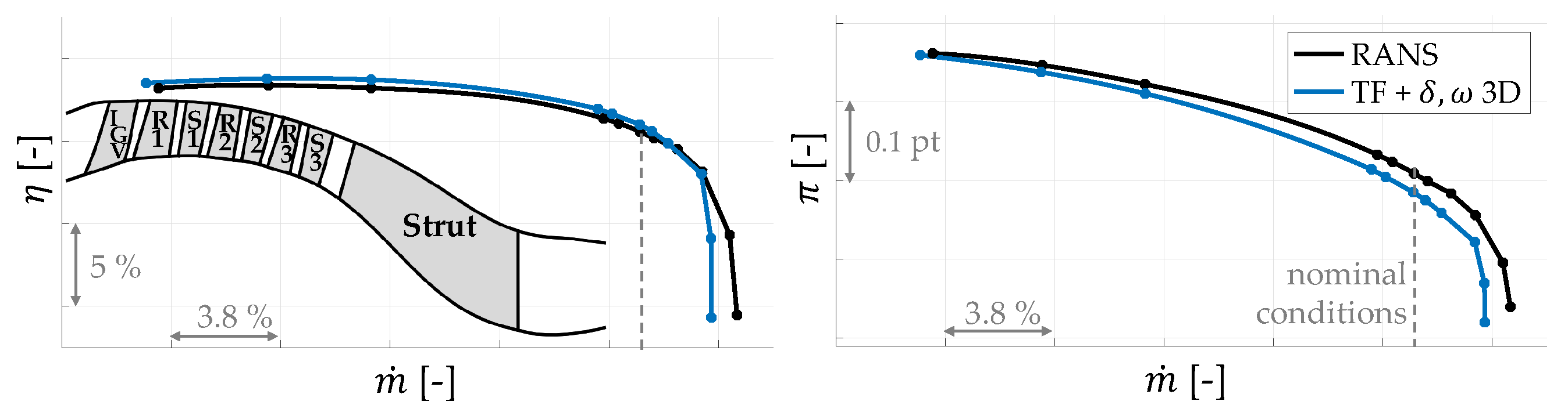
2.2.3. Solver Assessment

To validate the solver, through-flow simulations of a modern low-pressure compressor designed by Safran Aero Boosters are compared to the corresponding RANS simulations with a mixing plane approach using elsA. This highly loaded compressor features a high Mach number but still subsonic flow, and its endwalls undergo an important radius variation. It is composed of three stages of 3D modern blades between an inlet guide vane (IGV) and a strut, as depicted in Figure 2. The mesh is composed of about 40,000 cells. Simulations have been run for several values of the outlet pressure at nominal speed using a valve law to predict the performance for a set of mass-flow rates. The TF simulations are fed with the exact radial distribution of the key parameters ${\delta }_{\mathrm{TE}}$ and $\omega$ from the corresponding high-fidelity computations in order to isolate the modeling error from correlation empiricism. The deviation angle $\delta$ is usually defined at the blade trailing edge but is used here for the entire blade surface to account for the boundary layer on the blade wall. To obtain the deviation angle field $\delta$ everywhere in the blade, it is chordwise interpolated along streamlines from $\delta =0$ at the LE to its (radially distributed) value ${\delta }_{TE}$ at the TE. The loss coefficient is kept constant along streamlines as it is computed from blade LE and TE positions. Through this analysis, we assess the through-flow model with respect to its underlying assumptions prior to evaluating its ability to predict geometric variability effects.

The comparison of compressor performance, evaluated with respect to the first row inlet and last row outlet stations, is shown in Figure 2. The results are non-dimensionalized by reference values related to the operating conditions for confidentiality reasons. The through-flow simulations provide accurate results along the overall performance curves, while such a model is usually used to predict only nominal conditions at early design iterations. The mean epistemic error margin based on an L2 norm is around 2%, and the run time of the through-flow simulation is at least two orders of magnitude lower than the corresponding RANS simulation. The relative difference for the total pressure ratio slightly increases as the mass-flow rate increases. This small disagreement between the performance predictions is mainly due to the circumferential stress that is intrinsically included in the RANS computations but neglected by the through-flow model. In addition to this, rotor tip clearance and leakage flow cavity are currently not represented in the through-flow path. Their impact is only partially included in the prescribed parameter distribution. Finally, a more realistic stream-wise distribution of the key parameters ${\delta }_{\mathrm{TE}}$ and $\omega$ could also improve the prediction, as shown by Pacciani et al. [11].

At low mass-flow rates, the performance characteristics are limited by the non-convergence of both computational codes close to the same (numerical) stall onset point. The through-flow model is also able to accurately predict the maximum efficiency peak. However, at high mass-flow rate, the choking condition is achieved for a slightly lower mass-flow rate than RANS prediction. As explained by Baralon et al. [8] and Simon [7], a circumferential blockage, although consistent with the averaged governing equations, can lead to poor quality of the solution in the analysis mode when the performance is sought knowing the real geometry. An alternative formulation called “normal” blockage proposed in place of the circumferential one and computed with respect to the stream-wise direction in the blade-to-blade plane should be implemented to improve the captured choking mass-flow rate. In conclusion, it has been shown that the through-flow model is able to reproduce the 3D steady averaged flow field fairly well under the aforementioned assumptions provided that the key parameter distributions of ${\delta }_{\mathrm{TE}}$ and $\omega$ are precisely known (e.g., from high-fidelity data).

2.3. Correlations

The radial distributions of the deviation angle ${\delta }_{\mathrm{TE}}$ and loss coefficient $\omega$ are usually unknown and are therefore obtained from empirical correlations. In the context of a multi-fidelity approach, where TF and 3D RANS are combined, loss correlations could be learned from the RANS simulations. However, correlations adapted for modern engine designs, i.e., with highly loaded three-dimensional blades, are often kept confidential. As a consequence, the span-wise profiles of ${\delta }_{\mathrm{TE}}$ and $\omega$ are computed here using empirical correlations developed by Lieblein [20] and reported by Aungier [21]

$$\begin{array}{c}\hfill {\delta }_{\mathrm{TE}}\left(r\right)={\delta }_{\mathrm{TE}}^{*}+{\left[{\displaystyle \frac{\partial \delta }{\partial i}}\right]}^{*}\left(i-i^{*}\right)+10\left(1-{\displaystyle \frac{W_{m,\mathrm{TE}}}{W_{m,\mathrm{LE}}}}\right),\end{array}$$

(9a)

$$\begin{array}{c}\hfill \omega \left(r\right)=2{\displaystyle \frac{{\theta }_w\left(D_{eq}\right)}{c}}{\displaystyle \frac{\sigma }{cos{\beta }_{\mathrm{LE}}}}{\left({\displaystyle \frac{W_{\mathrm{TE}}}{W_{\mathrm{LE}}}}\right)}^2,\end{array}$$

(9b)

where i is the incidence angle, c the blade chord length, $\sigma$ the solidity, and ${\theta }_w$ the wake momentum thickness, which is computed as a quadratic function of the equivalent diffusion factor $D_{eq}$. The latter depends on the difference between the actual and the optimal incidence angle, $i-i^{*}$. For the deviation angle, the contribution at design conditions corresponds to the first term on the right-hand-side of Equation (9a) and is based on Carter’s rule [22]. The second term, representing the off-design contribution, is obtained using the methodology of Johnsen & Bullock [23] and Pollard & Gostelow [24], assuming a linear dependence on the incidence angle. The third term represents the dependence of the deviation angle on the axial velocity–density ratio (AVDR). For the loss coefficient, both design and off-design parts are included in the expression for ${\theta }_w$. Finally, a third correlation is used to compute the optimal incidence angle $i^{*}$, i.e., the incidence angle that achieves minimal loss [21]. More details can be found in the aforementioned references. Note that these correlations only account for two-dimensional profile losses generated in a blade-to-blade plane. Budo et al. [17] previously assessed their reliability on the CME2 compressor stage. TF predictions showed good global agreement over the full operating range. An example of the streamlines computed by the through-flow solver is reported in Figure 3, which clearly illustrates the flow turning achieved by the blade forces in both blade rows. Moreover, the endwall boundary layers are well represented in the stream surface as such a viscous formulation, unlike inviscid through-flow models, enables resolving the boundary layers on the annulus endwalls.

However, the adequacy of these correlations was previously shown to be poor when applied to modern compressors [17]. As illustrated in Figure 4, the through-flow prediction represented by the purple line shows significant underpumping compared to RANS. This phenomenon can be explained by the overestimation of the deviation angle at the rotor trailing edge, as highlighted in the right part of Figure 4, where the deviation angle law is plotted with respect to the incidence i. This overestimation is a consequence of the use of correlations obtained for two-dimensional blading used in early compressor technology studied at NACA. Therefore, modifications of the correlations have been introduced here in order to improve the prediction in the scope of this work. Specifically, the dominant term of the deviation angle correlation, that is, the slope parameter coming from Carter’s rule [22], has been modified. Moreover, Mach number effects, based on the work of [25], have been introduced in the loss coefficient correlation (Equation (9b)) because some underestimation of the loss had been noticed in Lieblein’s correlation [17]. As a result, the TF predictions (orange line in Figure 4) are drastically improved, and the performance curves show a satisfactory agreement. Although the agreement can be considered reasonable, the correlations should still be improved as the loss coefficient is underestimated at negative stall incidence. Moreover, the linear law predicted by the deviation angle correlation reproduces the deviation angle behavior fairly well in a range relatively close to the optimal incidence angle $i^{*}$, i.e., the incidence angle that achieved minimal loss, but completely fails to predict off-design conditions. This also suggests that, in a multi-fidelity design approach combining few 3D RANS with multiple TF simulations, the latter may be fed successfully with improved loss and deviation correlations based upon the RANS; this would greatly improve the reliability of the performance prediction by the TF solver, or at least ensure much better coherence with that obtained by RANS. Finally, the reliability of the through-flow results depends mostly on the accuracy of the deviation and loss models and their span-wise distribution.

2.4. Incidence Correction

Although satisfactory agreement is obtained between TF and RANS predictions, two additional modeling aspects that may impact the propagation of geometric variabilities at the blade leading edge must be taken into account. The first one is related to the axisymmetric assumption and the analysis mode: for a given flow incidence, the flow direction at the blade row inlet does not follow the camber line at the leading edge. However, the flow angle in the bladed region is imposed by the blade flow deflection force in the analysis mode. Consequently, a discontinuity occurs at the leading edge. This discontinuity leads to a sudden and non-physical increase in entropy and a spurious generation of losses, as shown in Figure 5. A numerical treatment is thus adopted to remove the flow discontinuity. The methodology consists of linearly modifying the mean flow path angle in the blade leading edge regions so that it adapts to the incident flow [8].

As shown in the figure, the fix is applied so that the stream surface modification due to incidence affects the first few percents of the blade chord. The blade geometry is thus locally modified by this numerical artifact. In the present work, a smoothing on the first 30% of the chord is used unless otherwise specified. A smaller chord portion leads to entropy generation and performance prediction error, while a longer portion impacts the geometry in too large a proportion. Even if this optimal choice introduces a low error in the global blade loading compared to the gain brought by more physical behavior of the loss generation, this modification of the blade geometry can also smooth any geometric variability in this region. Special attention should therefore be paid to this numerical artifact when propagating geometric uncertainties.

2.5. Camber Line Computation

The second aspect concerns the pre-processing of the blade geometry for TF simulations. Using prescribed velocity distribution design approaches, new highly optimized airfoils have been developed. Unlike NACA airfoils, which are parameterized based on a known line of mean camber, modern airfoils are directly defined by the position of the pressure and suction surface. However, TF simulations require a blade definition in terms of a mean camber line and a tangential thickness distribution for the blade force computation. In the vicinity of the leading edge, and trailing edge to a lesser extent, algorithms determining a mean camber line can be unreliable because the line of camber is no longer quasi-parallel with the section outline [9] and its definition is thereby not unique. As shown in the left part of Figure 6, the blade angle $\kappa$ can vary from 1 to 4 degrees close to the leading edge depending of the pre-processing tool. Although these tools are based on the same methodology, the LE treatment leads to dissimilar blade angle distributions, which may not be consistent with the blade loading distribution. The impact of this variability is relatively small, especially because the affected region is quite limited. Nonetheless, this epistemic uncertainty can exceed geometric variability in the leading edge region.

In order to assess the model sensitivity with respect to this uncertainty, TF simulations have been run based on the blade geometric outputs from two algorithms. The blade leading edge of each blade row computed by both algorithms varies from 1 to 4 degrees with respect to each other close to the leading edge. As shown in the right part of Figure 6, the direct impact of the blade angle distribution (blue lines) is low on the blade force if the correlation parameters ${\delta }_{\mathrm{TE}}$ and $\omega$ are known, i.e., taken from the RANS simulations here. Since the incidence correction smears the leading edge uncertainty, and losses and deviation do not depend at all on incidence since they are directly taken from the 3D rans, the predictions of the TF simulations are quite similar for the two blade angle distributions of Figure 6 (left). As proposed by [11], alternative smoothing formulations should be considered to decrease the leading edge stiffness. However, the empirical correlations for ${\delta }_{\mathrm{TE}}$, $\omega$, and, especially, $i^{*}$, use the actual geometry as input and are highly sensitive to the LE and TE blade angles. As a result, the blade angle uncertainty indirectly influences the blade forces through these correlations. It can be seen that, in this case, the TF model (orange lines in Figure 6 (right)) demonstrates large variability in its prediction. The methodology adopted here to alleviate this uncertainty consists of using the value of the blade angle outside the uncertainty region, i.e., at a few percents of the chord further downstream, as input for the calibrated correlations. The performance thus obtained corresponds to the orange line in Figure 4. An alternative solution could consist of extending the camber line in the region of interest according to a linear or higher-order law, consistent with the blade loading.

3. Analysis of the Effect of Geometric Variabilities

In this second part, we seek to assess the adequacy of the TF model, based on the improved correlations (orange line in Figure 4), to predict performance variations due to geometric variabilities. The overall goal is thus to determine through a sensitivity analysis how to best represent these geometric variations in the through-flow model and how the specific TF modeling aspects impact their propagation. The tuned TF model is used to quantify the relative variation in performance with respect to baseline conditions. The main quantities of interest (QoIs) to assess design robustness with respect to manufacturing variabilities are the mass-flow rate range, the total pressure ratio, and the isentropic efficiency. In the present preliminary analysis, the model ability to capture geometric variability effects is assessed only at nominal conditions because the correlations still need to be improved at high incidence conditions. Therefore, the stall margin is not considered here as a QoI. The aforementioned nominal conditions are defined as the intersection points between the operating line and the iso-speed line computed by the respective solvers, as shown in Figure 4. Since the baseline performance predicted by TF and RANS simulations differ due to modeling errors, the focus here is on the relative variation in performance with respect to nominal conditions predicted by the respective solvers so that their respective qualitative trends can be evaluated.

It is important to emphasize that, because of the axisymmetry assumption underlying the TF model and the assumed periodicity of the RANS reference simulations, geometric variabilities are intrinsically assumed to be identical on each blade of a given row, so the analysis of mistuned blade rows is not possible. Nevertheless, the relevance of the present study is motivated by the analysis of recurring systematic deformation patterns linked to tolerances and the blade manufacturing process. Mistuned blade rows could nonetheless be tackled by such an axisymmetric approach, in a statistical sense, by averaging the blade row geometries and by using propagation of the uncertainty/variation regarding blade geometry to the variation in performance. Another prospective approach to address mistuning could be the through-flow approach extended to three-dimensional body forces [26].

3.1. Manufacturing Variability

Geometric variations based on manufacturing variability parameters are propagated using the TF model. Only geometric variability based on the three-dimensional position of undeformed stator blades and through-flow geometry are discussed. These parameters, which are typically measured during industrial quality controls, are presented in the next section.

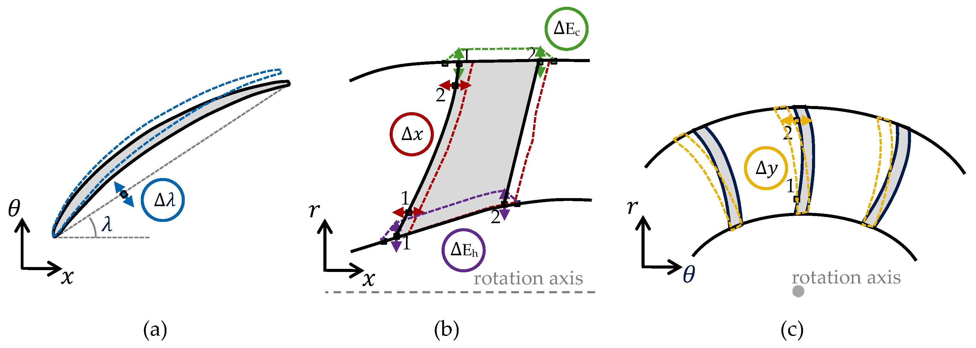
3.1.1. Imposed Geometric Variations

Five types of geometric variations on stator blade rows have been chosen to assess the TF model predictions. First, three degrees of freedom are related to the three-dimensional position of the undeformed stator blades, namely the variation in the stagger angle $\Delta \lambda$, the stream-wise ($\Delta x$), and pitch-wise ($\Delta y$) position keeping the blade geometry unchanged, as shown in Figure 7. Both $\Delta x$ and $\Delta y$ are defined by two contacts points, similarly to a mechanical feeler during quality controls. In the case of the circumferential position ($\Delta y$), only the relative position between contact points matters because of the row axisymmetry. The second set of degrees of freedom is related to linear endwall deformations, $\Delta E_h$ at the hub and $\Delta E_c$ at the casing, respectively. In particular, the endwalls, namely the hub and casing, are locally altered by displacing two control points on the walls in the vicinity of the blade leading and trailing edges. The control points are linearly connected to upstream and downstream reference points, as depicted in Figure 7b. The ranges of variability for the five degrees of freedom have been defined based on industrial tolerance limits and are summarized in

Table 1. Set of relative variations for each degree of freedom per stator blade row (IGV, S1, S2, and S3). The lengths and angles are non-dimensionalized by a mean chord $\overline{c}$ and a mean stagger angle $\overline{\lambda }$, respectively. The set of hub contour variations only contains the deformation $(2.85,-2.85)$ in the case of the S2 and S3 blades.

DOFs	Relative Variations [%]
$\Delta \lambda /\overline{\lambda }$	$-7.5;-3.75;7.5$
$(\Delta x_1,\Delta x_2)/\overline{c}$	$(1.7,1.7)$; $(1.7,-1.7)$
	$(-1.7,1.7)$; $(-1.7,-1.7)$
$(\Delta y_1-\Delta y_2)/\overline{c}$	$-4.3;-2.15;2.15;4.3$
$(\Delta E_{c1},\Delta E_{c2})/\overline{c}$	$(2.85,-2.85);(-2.85,2.85)$
$(\Delta E_{h1},\Delta E_{h2})/\overline{c}$	$(2.85,2.85)$; $(2.85,-2.85)$
	$(-2.85,2.85)$; $(-2.85,-2.85)$

. It should be emphasized that, among the 62 simulations, each geometric variation has been analyzed independently of the others; combined variations are not considered in the present work.

These geometric variations impact both the blade forces and correlations. As shown in Figure 8, the optimal incidence angle $i^{*}$ only depends on geometric parameters, namely the leading and trailing edge blade angle $\kappa$, the thickness-to-chord ratio ${\displaystyle \frac{t_{\max }}{c}}$, and the solidity $\sigma$, which are constant in the present case because the blade geometry itself remains unchanged. Therefore, $i^{*}$ is not impacted by the variabilities considered here. Similarly, the input geometric parameters of the correlations for ${\delta }_{\mathrm{TE}}$ and $\omega$ are independent of blade position variations, except for the radial coordinate that can slightly vary. As a result, both correlation outputs depend only indirectly on the geometric variations through the flow parameters, that is the optimal and actual incidence angle, the velocity components, the density, and the Mach number.

In addition to being influenced by potential correlation variations, the blade forces are directly impacted by the vector components normal and tangent to the blade camber surface. Specifically, the stream-wise variation $\Delta x$ perturbs the blade sweep designed to reduce the leading edge loading and secondary flows. Moreover, the leading edge is slightly misaligned with respect to the incident streamlines. As a consequence, the incidence conditions are slightly altered, as well as the correlation outputs. Moreover, the meridional variation in the blade row position is fully captured by a TF computation. Stagger angle variations mainly impact the localized blade twist and thereby the blade span-wise alignment with the flow, while the blade twist was precisely calibrated to reduce the high incidences in the endwall regions. These high-incidence conditions can be predicted in the endwall regions with a viscous TF solver. However, the profile loss correlation should be complemented by a secondary loss model to take full advantage of this TF feature.

The pitch-wise perturbation impacts the blade lean, which changes the span-wise distribution of the stage reaction and the mass-flow rate through the radial pressure gradient and the streamline curvature. The circumferential and radial components of the blade force are thus impacted so that the pressure close to the endwalls is increased and the fluid is deflected toward mid-span sections. This effect is axisymmetric and fully captured by a through-flow computation. The lean is also supposed to control secondary flows, specifically the corner vortex. However, this effect is not expected to be captured by the model because secondary losses are not included in the TF model due to their non-axisymmetric nature. Finally, the endwall deformation is mainly felt by the boundary layer and thus the turbulence model. It also impacts the computation of the correlations through the variation in the flow conditions.

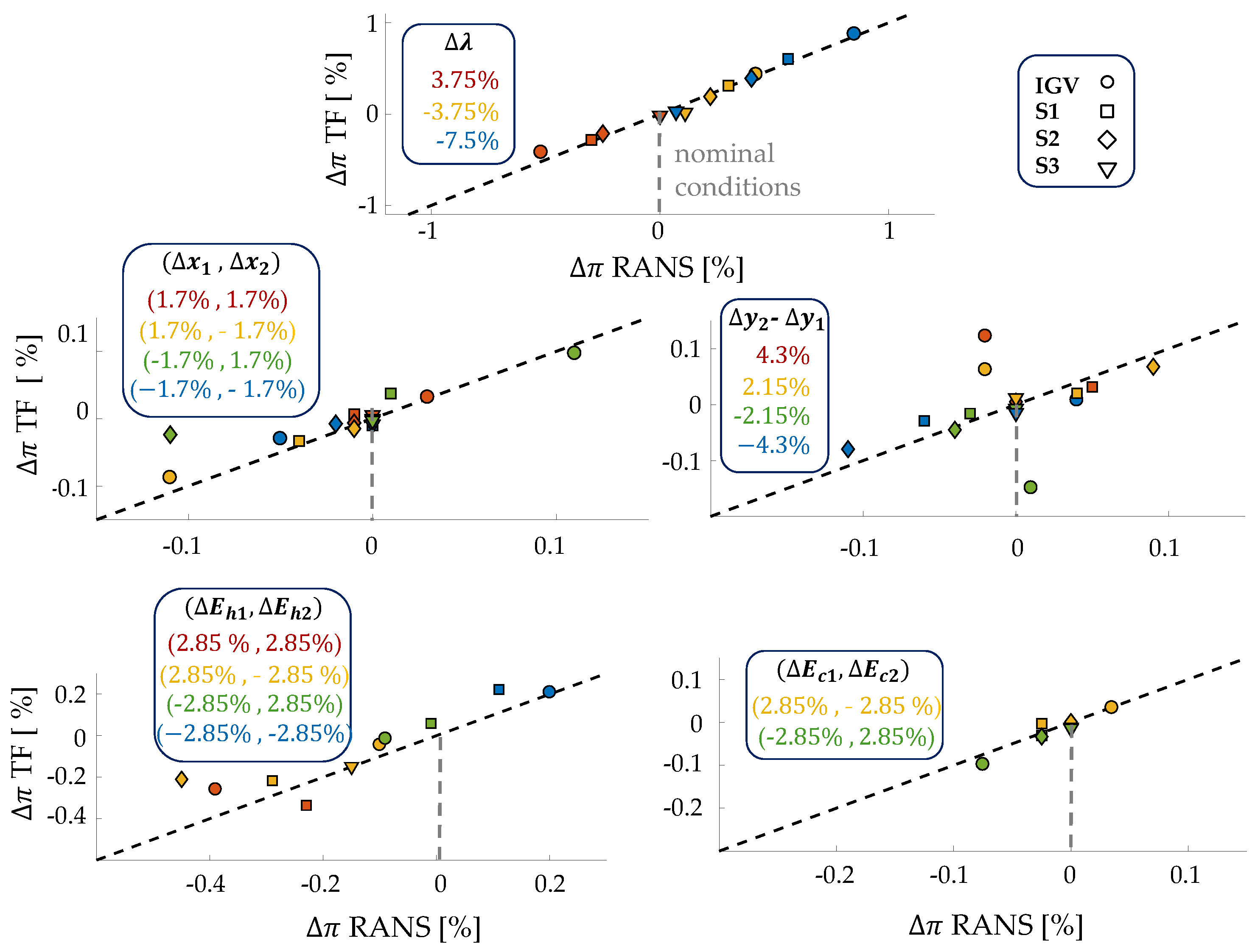
3.1.2. Sensitivity Analysis

The variation in the quantities of interest with respect to the imposed manufactured perturbations at nominal conditions is summarized for all cases in Figure 9. The results show good global agreement between the trends predicted by RANS (closed symbols) and TF (open symbols) models, except for cases where the difference is of the same order as the performance variation. The mean absolute difference between relative performance variation in both solvers is equal to 0.0065%, 0.0074%, and 0.0017% for the mass-flow rate, the total pressure ratio, and the isentropic efficiency, respectively. The error for the efficiency variation seems lower, but the variation range is three times lower than for other quantities. Consequently, the relative errors are of the same order of magnitude.

The total pressure ratio mostly exhibits a linear variation with respect to the mass-flow rate, while the variations in the isentropic efficiency are more scattered around its baseline value. This linear behavior can be explained by the boundary conditions used in both the RANS and TF simulations: at the outlet, the flow is smoothed as the symmetric strut mostly forces an axial flow at its trailing edge. Therefore, the radial equilibrium predicts a static pressure distribution that is almost uniform, and the pressure level is prescribed by the reference pressure. On the other hand, the mass-flow rate is proportional to the total-to-static pressure ratio at the outlet station. Therefore, the mass-flow rate and the total pressure ratio are a function of only the outlet total pressure as the total pressure and the static pressure are imposed at the inlet and the outlet stations, respectively. As a result, for a given compression load, more efficient work leads to an increase in both mass-flow rate and total pressure ratio. In the case of the isentropic efficiency, additional parameters related to loss mechanisms come into play.

With regard to the respective contributions of the variability parameters, the stagger angle seems to have the greatest impact, while the variations in the blade axial position seem to have the lowest importance. However, the relative importance of the impact of each geometric parameter can be misleading because their range of variation is different and their relative variation to the nominal value is also different. It is therefore more relevant to compare the impact of each geometric parameter separately, as shown in Figure 10. For the sake of clarity, only the total pressure ratio variations in both solvers are reported. A modification of the most upstream blade row has the highest impact on the performance because the resulting perturbed flow impacts all downstream blade rows in cascade and changes their incident flow conditions. Consequently, the performance of the downstream blade rows is also altered. The global trend is accurately captured by the TF model as the scatter points closely align with the linear correlation law. The accuracy of the quantitative performance variation is a bit lower in the case of endwall deformation as the TF model does not include a secondary flow model. Moreover, the deficiencies of turbulence models can also play a role in this flow region.

Finally, the variations in the correlation parameters ${\delta }_{\mathrm{TE}}$ and $\omega$ of the S1 blade with respect to imposed geometric variability on the S1 blade are shown in Figure 11. Moreover, the total loss coefficient ${\omega }_t$, which includes the profile loss from correlations for $\omega$ and endwall loss from the turbulence model, is also presented. It is computed from the flow-field quantities as

$${\omega }_t={\displaystyle \frac{p_{t,is,\mathrm{LE}}-p_{t,\mathrm{TE}}}{p_{t,\mathrm{LE}}-p_{\mathrm{LE}}}}.$$

(10)

The individual plots indicate that the flow variance is essentially caused by the stagger angle and endwall perturbations. The impact of endwall deformations is consistently felt by the flow in a region close to the hub and casing. These effects are partly driven by the turbulence model in viscous TF equations. Due to the variation in the deviation angle, performance variations are mostly felt by the downstream blade rows, which experience inlet flow variations.

Figure 10. Relative pressure ratio variations due to stagger angle variation (top), meridional displacement (center left), pitch-wise displacement (center right), and hub and casing deformation at nominal operation conditions (bottom). Correlations between RANS and though-flow (TF) simulations where only a parameter is modified per blade row and per simulation.

Figure 10. Relative pressure ratio variations due to stagger angle variation (top), meridional displacement (center left), pitch-wise displacement (center right), and hub and casing deformation at nominal operation conditions (bottom). Correlations between RANS and though-flow (TF) simulations where only a parameter is modified per blade row and per simulation.

Figure 11. Variation in the deviation angle ${\delta }_{\mathrm{TE}}$ (Equation (9a)), profile loss coefficient $\omega$ (Equation (9b)), and total loss coefficient ${\omega }_t$ (Equation (10)) along the blade span h with respect to imposed geometric variability on the S1 blade.

Figure 11. Variation in the deviation angle ${\delta }_{\mathrm{TE}}$ (Equation (9a)), profile loss coefficient $\omega$ (Equation (9b)), and total loss coefficient ${\omega }_t$ (Equation (10)) along the blade span h with respect to imposed geometric variability on the S1 blade.

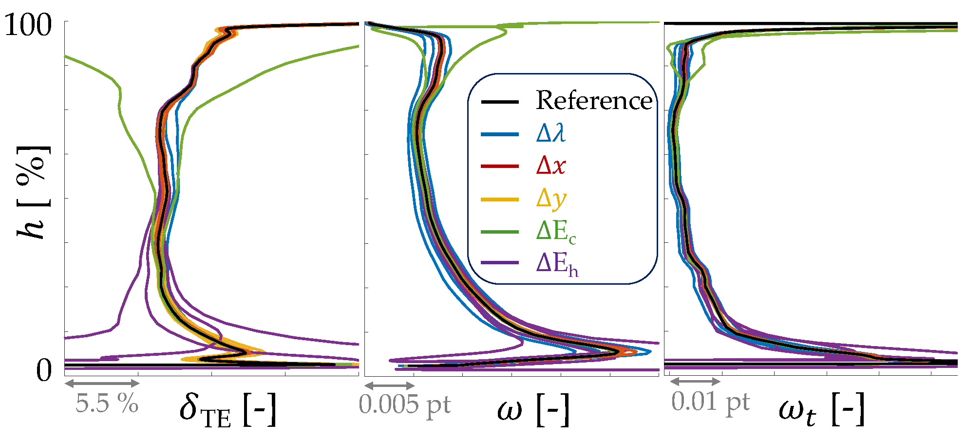
3.2. Evaluation of the Effects of Modeling Aspects on Variability Impact at Leading Edge

Despite the promising results reported above, the impact of other types of geometric variability can still be partially smoothed by the model due to the approximations and empiricism inherent to the TF solver. The leading edge is a critical example as the aforementioned modeling aspects directly impact the propagation of geometric variability precisely in this region. This section thus aims to evaluate the ability of the through-flow modeling approach to quantify the impact of geometric variabilities at the leading edge. First, the camber line at the blade leading edge is modified by $\pm 1.5°$ over the first 20% of the chord along the blade span. For each simulation, only one blade row is modified. The comparison of the compressor performance variations obtained with TF and RANS, respectively, is shown in Figure 12. As explained above, a blade geometry modification at the leading edge is mainly felt through the correlations for ${\delta }_{\mathrm{TE}}$ and $\omega$ because the LE blade angle is one of the main input parameters for these correlations, as shown in Figure 8. As a result, the model is able to predict performance variation with respect to this geometric variability. The global trend is effectively captured by the TF model, although not as accurately as in previous variability tests: the relative performance variation is largely overestimated by the TF solver, meaning that the epistemic uncertainty stemming from the aforementioned aspects provides a large contribution in this case.

4. Conclusions

This paper presents the evaluation of a viscous CFD-based through-flow solver and its adequacy to predict geometric variability effects on compressor performance, in continuity with the work conducted in two previously published conference papers [27,28]. A modern highly loaded multi-stage axial low-pressure compressor designed by Safran Aero Boosters is used as a test-case to assess the reliability of the method. It has been shown that the distribution of key parameters, the deviation angle ${\delta }_{\mathrm{TE}}$ and the loss coefficient $\omega$, is critical as a good prediction of them provides a very good match between RANS and TF, as shown by a priori tests using RANS input data. Standard correlations from the literature have shown to perform poorly on modern compressors. Improved empirical correlations for these two parameters have thus been introduced by the authors, but the updated correlations are still not very accurate, leading to non-negligible discrepancies between RANS and TF simulations. Moreover, the incidence correction needed to mitigate the spurious entropy increase at the blade leading edge and the camber line computation have a significant impact on the performance prediction. The former tends to smooth any geometric variability in this region. The latter has a significant impact on the deviation angle and loss coefficient predicted by the empirical correlations. The propagation, and thus the evaluation, of geometric uncertainties are marred by additional epistemic uncertainties inherent to the TF model. Hence, strategies have been proposed to mitigate these model uncertainties. Finally, a preliminary study indicates that the TF model provides realistic predictions of performance variations due to the effect of imposed geometric changes except at the blade leading edge, where the epistemic uncertainty stemming from the aforementioned aspects has a large contribution in this case. The results are promising, and future work should assess the model prediction with respect to other types of blade deformation. Note that, due to the axisymmetry assumption on which the TF model is based, as the periodicity of the simulations of reference (RANS), geometric variabilities are intrinsically identical on each blade of the row, which is incompatible with mistuned blade row analysis. Nevertheless, the relevance of the present study is motivated by the analysis of recurring deformation patterns linked to tolerances and the blade manufacturing process. Mistuned blade rows would be tackled by such an axisymmetric approach though, averaging the blade row geometries.

References

1. Dow, E.A.; Wang, Q. The Implications of Tolerance Optimization on Compressor Blade Design. J. Turbomach. 2015, 137, 101008. [Google Scholar] [CrossRef]
2. Bestle, D.; Flassig, P. Optimal Aerodynamic Compressor Blade Design Considering Manufacturing Noise. In Proceedings of the ISSMO Conference, London, UK, 8–9 July 2010. [Google Scholar]
3. Garzon, V.E.; Darmofal, D.L. Impact of Geometric Variability on Axial Compressor Performance. J. Turbomach. 2003, 125, 692–703. [Google Scholar] [CrossRef]
4. Nigro, R. Uncertainty Quantification for Robust Design of Axial Compressors. Ph.D. Thesis, University of Mons, Mons, Belgium, 2018. [Google Scholar]
5. Lange, A.; Voigt, M.; Vogeler, K.; Johann, E.; Royce, R.; Kg, C.; Dahlewitz, D. Principal Component Analysis On 3D Scanned Compressor Blades For Probabilistic CFD Simulation. In Proceedings of the AIIA Conference, Granada, Spain, 3–7 September 2012; pp. 1–16. [Google Scholar] [CrossRef]
6. Goodhand, M.N.; Miller, R.J.; Lung, H.W. The Impact of Geometric Variation on Compressor Two-Dimensional Incidence Range. J. Turbomach. 2014, 137, 021007. [Google Scholar] [CrossRef]
7. Simon, J.F. Contribution to Throughflow Modelling for Axial Flow Turbomachines. Ph.D. Thesis, University of Liège, Liège, Belgium, 2007. [Google Scholar]
8. Baralon, S.; Erikson, L.E.; Hall, U. Validation of a Throughflow Time-Marching Finite-Volume Solver for Transonic Compressors. In Proceedings of the ASME Turbo Expo, Stockholm, Sweden, 1–4 June 1998. [Google Scholar]
9. Lange, A.; Vogeler, K.; Gümmer, V.; Schrapp, H.; Clemen, C. Introduction of A Parameter Based Compressor Blade Model For Considering Measured Geometry Uncertainties In Numerical Simulation. ASME J. Turbomach. 2009, 48876, 1113–1123. [Google Scholar]
10. Wu, C.H. A General Theory of Three-Dimesional Flow in Subsonic and Supersonic Turbomachines of Axial-, Radial-, and Mixed-Flow Types; Technical Report; NACA: Washington, DC, USA, 1952. [Google Scholar]
11. Pacciani, R.; Rubechini, F.; Marconcini, M.; Arnone, A.; Cecchi, S.; Daccà, F. A CFD-based throughflow method with an explicit body force model and an adaptive formulation for the S2 streamsurface. Proc. Inst. Mech. Eng. Part A J. Power Energy 2016, 230, 16–28. [Google Scholar] [CrossRef]
12. Righi, M.; Pachidis, V.; Könözsy, L.; Pawsey, L. Three-Dimensional Through-Flow Modelling of Axial Flow Compressor Rotating Stall and Surge. Aerosp. Sci. Technol. 2018, 78, 271–279. [Google Scholar] [CrossRef]
13. Föllner, S.; Amedick, V.; Bonhoff, B.; Brillert, D.; Benra, F.K. Model validation of an Euler-based 2D-Throughflow Approach For multistage Axial Turbine Analysis. In Proceedings of the ASME Turbo Expo, London, UK, 22–26 June 2020; Volume 29, pp. 185–186. [Google Scholar]
14. Jian, L.; Dongrun, W.; Jinfang, T.; Mingmin, Z.; Xiaoqing, Q. The Effects of Incidence and Deviation on the CFD-Based Throughflow Analysis. In Proceedings of the ASME Turbo Expo, London, UK, 22–26 June 2020; pp. 1–9. [Google Scholar]
15. Adamczyk, J.J. Model Equation for Simulating Flows in Multistage Turbomachinery; Technical Report TM-86869; NASA: Cleveland, OH, USA, 1984. [Google Scholar]
16. Adamczyk, J.J. Aerodynamic Analysis of Multistage Turbomachinery Flows in Support of Aerodynamic Design. ASME J. Turbomach. 1999, 122, 189–217. [Google Scholar] [CrossRef]
17. Budo, A.; Terrapon, V.E.; Arnst, M.; Hillewaert, K.; Mouriaux, S.; Rodriguez, B.; Bartholet, J. Application of a Viscous Through-Flow Model to a Modern Axial Low-Pressure Compressor. In Turbo Expo: Power for Land, Sea, and Air. American Society of Mechanical Engineers; American Society of Mechanical Engineers: New York City, NY, USA, 2021. [Google Scholar] [CrossRef]
18. Smith, B.R. A Near Wall Model for The k-l Two Equation Turbulence Model. In Proceedings of the AIIA Conference, Austin, TX, USA, 31 May–3 June 1994; pp. 1–8. [Google Scholar] [CrossRef]
19. Jameson, A.; Schmidt, W.; Turkel, E. Numerical solution of the Euler equations by finite volume methods using Runge Kutta time stepping schemes. In Proceedings of the 14th Fluid and Plasma Dynamics Conference, Palo Alto, CA, USA, 23–25 June 1981. [Google Scholar]
20. Lieblein, S. Incidence and Deviation-Angle Correlations for Compressor Cascades. ASME J. Turbomach. 1960, 82, 575–584. [Google Scholar] [CrossRef]
21. Aungier, R.H. Axial-Flow Compressors; The American Society of Mechanical Engineers: New York City, NY, USA, 2003. [Google Scholar]
22. Carter, A. The Low Speed Performance Of Related Aerofoils In Cascades; Technical Report 19; Aeronautical Research Council: London, UK, 1950. [Google Scholar]
23. Johnsen, I.; Bullock, R. Aerodynamic Design of Axial-Flow Compressors; Number SP-36; NASA: Washington, DC, USA, 1965; pp. 1–507. [Google Scholar]
24. Pollard, D.; Gostelow, J.P. Some Experiments at Low Speed on Compressor Cascades. J. Eng. Gas Turbines Power 1967, 89, 427–436. [Google Scholar] [CrossRef]
25. Kónig, W.M.; Hennecke, D.K.; Fottner, L. Improved Blade Profile Loss And Deviation Angle Models For Advanced Transonic Compressor Bladings: Part I—A Model For Subsonic Flow. ASME J. Turbomach. 1994, 118, 73–80. [Google Scholar] [CrossRef]
26. Cao, T.; Hield, P.; Tucker, P.G. Hierarchical Immersed Boundary Method with Smeared Geometry. J. Propuls. Power 2017, 33, 1151–1163. [Google Scholar] [CrossRef]
27. Budo, A.; Hillewaert, K.; Bartholet, J.; Terrapon, V.E. Assessment of geometrical variability effects through a viscous through-flow model applied to modern axial-flow compressor blades. In Proceedings of the 15th European Conference on Turbomachinery Fluid Dynamics and Thermodynamics, Budapest, Hungary, 24–28 April 2023; Available online: https://www.euroturbo.eu/publications/proceedings-papers/etc2023-307/ (accessed on 1 November 2024).
28. Budo, A.; Hillewaert, K.; Arnst, M.; Le Man, T.; Terrapon, V.E. Quantification of geometric variability effects through a viscous through-flow model: Sensitivity analysis of the manufacturing tolerance effects on performance of modern axial-flow compressor blades. In Turbo Expo: Power for Land, Sea, and Air; American Society of Mechanical Engineers: New York City, NY, USA, 2023; Available online: https://asmedigitalcollection.asme.org/GT/proceedings-pdf/GT2023/87103/V13CT32A023/7045776/v13ct32a023-gt2023-102800.pdf (accessed on 1 November 2024). [CrossRef]
Figure 1. Adamczyk’s cascade: levels of modeling used to simulate turbomachine flows [16].
Ijtpp 10 00006 g001
Figure 2. Isentropic efficiency η (left) and total pressure ratio π (right) as a function of the normalized mass-flow rate at the nominal rotational speed and meridional sketch of the compressor (left). Comparison of RANS and through-flow simulations fed with exact correlation parameters from RANS computations.
Ijtpp 10 00006 g002
Figure 3. Axisymmetric-averaged streamlines for the CME2 stage in nominal regime ( m ˙ = 10.5 kg / s ), with Mach number contours and fictitious positions of the rotor (R) and stator (S) blades.
Ijtpp 10 00006 g003
Figure 4. Total pressure ratio as a function of the mass-flow rate at the nominal rotational speed of the compressor (left). Comparison of RANS and through-flow simulations with different computed key parameters. Qualitative behavior of key parameter δ TE and ω laws with respect to incidence i (right).
Ijtpp 10 00006 g004
Figure 5. Entropy generation due to leading edge discontinuity for different extents of the incidence smoothing and sketch of the smoothed blade geometry (left). Corresponding total pressure ratio (point data) at the nominal regime and maximum peak efficiency (right).
Ijtpp 10 00006 g005
Figure 6. Blade angle distribution along the chord (left) and total pressure ratio as a function of the mass-flow rate (right) at the nominal rotational speed of the compressor for two airfoil splitting algorithms (dotted and dashed lines). Comparison of RANS (black line) and through-flow simulations with different computed key parameters (blue and orange lines).
Ijtpp 10 00006 g006
Figure 7. Sketch of the geometric degrees of freedom in (a) the blade-to-blade, (b) meridional, and (c) front planes: three-dimensional blade rigid motions and linear endwall deformation. The dotted colored lines illustrate the corresponding modified geometry for a positive deviation with respect to the baseline.
Ijtpp 10 00006 g007
Figure 8. Dependencies of blade forces and correlation outputs with respect to geometric and flow quantities. The geometric variations imposed are indicated by the shaded box.
Ijtpp 10 00006 g008
Figure 9. Relative pressure ratio, isentropic efficiency, and mass-flow-rate variations due to geometric variabilities at nominal operation conditions. Comparison of RANS (closed symbols) and though-flow (open symbols) simulations where only a parameter is modified per blade row and per simulation. The black lines are the iso-speed performance curves of reference.
Ijtpp 10 00006 g009
Figure 12. Changes in pressure ratio due to LE blade angle κ variations. Correlations between RANS and TF simulations for each time a single blade row is modified.
Ijtpp 10 00006 g012