Article

Comparison of Seasonal and Diurnal Concentration Profiles of BVOCs in Coniferous and Deciduous Forests

1
Department Monitoring and Exploration Technologies, UFZ Helmholtz Centre for Environmental Research, Permoserstraße 15, 04318 Leipzig, Germany
2
Chair of Forest Protection, Department of Forest Sciences, Technische Universität Dresden, Pienner Straße 8, 01737 Tharandt, Germany
3
Department of Computational Hydrosystems, UFZ Helmholtz Centre for Environmental Research, Permoserstraße 15, 04318 Leipzig, Germany
*
Author to whom correspondence should be addressed.
Atmosphere 2023, 14(9), 1347; https://doi.org/10.3390/atmos14091347
Submission received: 19 June 2023 / Revised: 9 August 2023 / Accepted: 23 August 2023 / Published: 26 August 2023

Abstract

:
Ambient atmospheric concentrations of isoprene and monoterpenes were measured at two forest sites, one deciduous and one coniferous, over the year 2022. Both sites in a regional area were sampled monthly between April and September. The samples were taken using sorbent tubes and analyzed with thermal desorption–gas chromatography–mass spectrometry. The highest concentrations were determined in August at both sites. While isoprene is the most abundant compound at the deciduous forest with an average concentration of 5.59 µg m−3 in August, α-pinene and β-pinene dominate throughout the year at the coniferous forest with the highest concentrations also in August (3.44 µg m−3 and 1.51 µg m−3). Because other monoterpenes (camphene, sabinene, 3-carene, p-cymene and limonene) are also emitted in significant amounts, the total concentration measured in the coniferous forest is higher (7.96 µg m−3 in August) in comparison to the deciduous forest (6.08 µg m−3). Regarding the detected monoterpenes in the deciduous forest, sabinene is the dominant monoterpene in addition to α-pinene and is sometimes present in higher (July) or equal (August) concentrations. The seasonal and diurnal concentrations of all monoterpenes correlate very well with each other at both sites. An exception is sabinene with a diurnal concentration profile similar to isoprene.

1. Introduction

Biogenic volatile organic compounds (BVOCs) have a significant influence on atmospheric chemistry [1]. They are important precursors of ozone. BVOCs react with hydroxyl radicals and form peroxy radicals, which undergo further reactions with nitric oxide forming nitrogen dioxide, organic nitrate or alkoxy radicals. Ultimately, ozone is formed from nitrogen dioxide via photolysis [2]. On the other hand, gas-phase reactions of BVOCs with ozone, hydroxyl or nitrate radicals lead to the formation of oxygenated products. These compounds have a lower vapor pressure in comparison to BVOCs, leading to condensation and the formation of secondary organic aerosols (SOAs) [3]. SOAs represent a significant fraction of atmospheric particulate matter which can influence air quality and climate radiative forcing [4].
A dominant fraction of BVOCs originates from vegetation emissions. A total of 90% of total global non-methane VOCs are attributed to this emission source [5]. Isoprene and monoterpenes are compounds which are emitted in large amounts from forest areas. Different modelling approaches were developed for the prediction of BVOC flux [6]. Using these models, global emission rates of isoprene were postulated with ~450–600 Tg C year−1 [7], while global terpene emissions were estimated at 175 Tg C year−1 [8].
Isoprene and monoterpenes are formed within plants via two synthesis pathways: the mevalonic acid pathway which takes place in the microsomes and cytoplasm and the methylerythritol phosphate pathways which takes place in chloroplasts [9]. Isopentenyl pyrophosphate (IPP) and its isomer dimethylallyl pyrophosphate (DMAPP) are formed as intermediates in both pathways. Isoprene is produced by the elimination of pyrophosphate from DMAPP. The formation of monoterpenes takes place via the formation of the precursor geranyl diphosphate from IPP and DMAPP, and subsequent dephosphorylation [10]. Generally, some of the BVOCs are constitutively formed. They are already synthesized and either stored in storage pools and resin ducts or directly emitted. Another part of BVOCs, the inducible forest BVOCs, are synthesized de novo after herbivore attacks or under abiotic stress [8].
The emission of the formed BVOCs from plants takes place in different ways. Light-dependent or de novo biosynthesis emissions are those where the compounds are emitted through the plant stomata shortly after their formation. Especially isoprene and some monoterpenes are emitted in this manner, while most monoterpenes are volatilized from storage pools or resin ducts of plants in a temperature-dependent manner [11].
Due to these different emission pathways, the seasonal and diurnal variation of concentration profiles of individual compounds varies. However, the temporal changes of the concentration profiles are much more complex and variable, because other factors also have a considerable influence on emission rates. The geographical location (tropical, temperate or boreal forests), plant internal factors (tree species, tree age, and plant development stage), site characteristics (soil properties, and nutrient availability), environmental factors (humidity, temperature, and solar radiation) and stress factors including biotic stress (plant defense mechanisms against pathogens, herbivores or insect attacks) and abiotic stress (drought stress, air pollution, and concentrations of carbon dioxide and ozone) are parameters affecting the emission rates of BVOCs [5,9]. Furthermore, some monoterpenes have high reactivities in the presence of atmospheric oxidants and therefore a limited atmospheric lifetime [12].
For these reasons, modeling approaches for the prediction of emissions are difficult and subject to very large uncertainties [13]. Also, measured atmospheric concentrations are highly variable in the literature [14,15,16]. The seasonal and diurnal concentration profiles are well investigated for only a few compounds. Data sets for the simultaneous study of deciduous and coniferous forests in a regional area are not known from the literature.
Isoprene, which is emitted in a light-dependent manner, shows a strong daytime emission with the highest concentration midday to late afternoon, while the nighttime emission goes down to near zero. The atmospheric concentrations of monoterpenes, which are emitted in a temperature-dependent manner, are often the greatest during the nighttime hours due to the shrinking of the planetary boundary layer. Furthermore, the concentration decreases during the day with a high intensity of incoming solar radiation due to oxidation by photochemically formed radicals [17,18] or the reduction in enzyme activity when the leaf temperature is too high. However, not all monoterpenes show a comparable emission behavior and it is not completely clear in which way the individual monoterpenes are emitted from vegetation [11]. Consequently, long-term measurements of BVOCs can assist in understanding these different emission pathways.
Therefore, we investigated the seasonal and diurnal variations of the ambient atmospheric concentrations of isoprene and monoterpenes over one year at two sampling sites, a deciduous forest and a coniferous forest, using active sampling with multiphase adsorbent tubes and subsequent analysis by thermal desorption—gas chromatography—mass spectrometry (TD-GC-MS). Our aim was to understand in which way the emission pathways known from the literature correlate with the ambient BVOC concentrations. Therefore, the measured concentrations were correlated with factors potentially affecting the concentration profile of isoprene and monoterpenes, such as temperature, photosynthetically active radiation, relative humidity, windspeed, soil water content and soil temperature measured during the sampling periods.

2. Materials and Methods

2.1. Sampling Sites

The samples were taken monthly at the same time at two locations in Germany about 200 km away from each other. The sampling site Hohes Holz is located in a deciduous forest while the site Tharandt is an extended coniferous forest area. Both sampling sites belong to the European research infrastructure ICOS (Integrated Carbon Observation System).
The sampling site Hohes Holz is located in the German state of Saxony-Anhalt, approximately 35 km west of the state capital Magdeburg with the following coordinates in WGS84 system (World Geodetic System 1984): Latitude 52.08656° N, Longitude 11.22235° E. The elevation above sea level is 193 m. The dominant species of the forest are as follows: European beech (Fagus sylvatica L.), sessile oak (Quercus petraea (Matt.) Liebl.), silver birch (Betula pendula Roth), common hornbeam (Carpinus betulus L.), and in afforestations, European spruce (Picea abies (L.) H. Karst.) and European larch (Larix decidua Mill.).
The sampling site Tharandt is located in the German state Saxony about 25 km southwest of the state capital Dresden. The site is an evergreen needleleaf forest in the lower region of the Eastern Ore Mountains with the following coordinates: Latitude 50.96256° N, Longitude 13.56515° E. The elevation of this site is 380 m above the sea level. The present species are composed of 97% coniferous trees (72% European spruce (Picea abies (L.) H. Karst.), 15% Scots pine (Pinus sylvestris L.), 10% European larch (Larix decidua Mill.) and 3% deciduous trees (1% birches (Betula spec.) and 2% others).
The photosynthetically active radiation (PAR, 400 to 700 nm) was measured using a quantum sensor (LI-190SZ, LI-COR, Lincoln, Dearborn, MI, USA) at both sites, and the air temperatures using a PT100 temperature probe (FISCHER Mess- und Regeltechnik GmbH, Bad Salzuflen, Germany).

2.2. Sampling

The samples were taken using multiphase adsorbent tubes (Bio-monitoring stainless-steel tubes, Markes International Ltd., Bridgend, UK) consisting of Tenax TA and Carbograph 5TD. A total of 32 tubes were positioned in the MTS-32 multi-tube sequential sampler (Markes International Ltd., Bridgend, UK). The gas flow during the sampling was adjusted to 80 mL min−1 for 4 h, resulting in 19.2 L of preconcentrated air per tube. During each measurement campaign, 32 tubes were sampled in sequence, giving a total observation time of 5 days and 8 h. The samplers for automated air collection were placed mid-canopy at a height of 13 m above ground level at the test site Hohes Holz, while the samples were taken at a height of 2 m at Tharandt.
All tubes were conditioned before use according to the recommendation of the manufacturer (2 h at 320 °C and 4 h at 330 °C) using a tube conditioner TC-20 (Markes International Ltd., Bridgend, UK). As known from the literature, the sampling of isoprene and terpenes can be influenced by ozone (O3). The O3 exposure during the sampling can lead to the formation of artifacts from Tenax [19] or causes losses of target compounds [20,21]. Therefore, the use of O3 scrubbers is necessary. Since the filters had to be integrated into the sampler, we developed compact O3 scrubbers based on potassium iodide, which were placed directly on the tubes. In addition to sodium thiosulfate [22] and manganese dioxide-coated copper nets [23], potassium iodide (KI) is a proven reagent for removing O3 which was successfully applied in different configurations such as copper tubes coated with KI [24], KI-impregnated glass wool [25] or in its crystalline form [26].
We impregnated sintered glass filter discs (ROBU Glasfilter-Geräte GmbH, Hattert, Germany) with KI (Merck KGaA, Darmstadt, Germany). The filter discs are made of borosilicate glass having a diameter of 6 mm and a pore size between 40–100 µm. A 10% aqueous KI solution was applied to the frits, dried and then integrated in self-made scrubber housings. They are placed airtight on the diffusion-locking caps (DiffLok caps, Markes International Ltd., Bridgend, UK) which seal the adsorption tubes. Between frit and cap, approximately 0.5 g of copper wool (Carl Roth, Karlsruhe, Germany) was placed for the reduction of reactive iodine products.

2.3. Analytical Procedure

The analytical method was developed and optimized based on the procedure of Helin et al. [27]. The loaded adsorbent tubes were desorbed using a TD100-xr multi-tube thermal desorber unit (Markes International Ltd., Bridgend, UK). First, the tubes were dry purged with a helium flow of 20 mL min−1 for 2 min before desorption. They were then heated to 300 °C for 5 min. The flow rate of helium during this primary desorption was 50 mL min−1 without split. The desorbed compounds were transferred to the focusing trap which is held at 20 °C. After finishing the primary desorption, the focusing trap is rapidly heated to 300 °C and held for 3 min. During this secondary desorption, the helium gas flow was 6 mL min−1. An amount of 1 mL min−1 of this gas flow was transferred to the gas chromatograph via a transfer line with a temperature of 200 °C. The split gas flow during the secondary desorption was 5 mL min−1. The samples were transported within the transfer line via a deactivated fused silica column which is connected to the gas chromatographic column (HP-5ms capillary column, 30 m length, 0.25 mm inner diameter, 0.25 µm film thickness, Agilent, Santa Clara, CA, USA). The oven temperature program was as follows: 35 °C (3 min)—5 K min−1—100 °C—15 K min−1—180 °C—20 K min−1—300 °C (2 min). The column flow rate of helium was 1 mL min−1.
The system was calibrated using external standards. The standard solution was prepared by mixing commercial solutions (Terpenes MegaMix, Restek, Bad Homburg, Germany) and weighed substances. A maximum of 20 microliters of methanolic solutions were injected in a CIS injection system (Gerstel, Mülheim an der Ruhr, Germany) at a temperature of 160 °C. The gas flow through the injector and adsorbent tube was realized using an air sampling pump (AMA, Karlsruhe, Germany) with a flow rate of 100 mL min−1. The sucked air was cleaned before the injector using charcoal filter systems.

2.4. Statistical Analysis

Statistical tests were performed in RStudio (v. 2022.12.0 + 353) using R (v.4.2.2) and ggplot2 (v. 3.4.0) to evaluate correlations between concentrations of BVOCs and environmental conditions during sampling. Spearman’s rank correlation was chosen since no linear relationship between concentrations and environmental conditions was expected.

3. Results

3.1. Effectiveness of the Ozone Scrubber

Before the field trials started, we investigated the efficiency of our developed O3 scrubbers. As described above, the presence of O3 can cause losses of terpenes during the sampling and degradation products can be formed from Tenax. Therefore, we investigated the recovery of terpenes after the preconcentration with and without the O3 scrubber. The liquid samples of target compounds were evaporated in a gas stream via permeation using a reference gas generator [28]. The generated sample gas flow was guided through the bio-monitoring tubes under the same conditions as used during the sampling in the field (preconcentration of 19.2 L sample gas stream with 80 mL min−1 for 4 h). The concentrations were adjusted to approximately 3 ng L−1 for α-pinene, 6 ng L−1 for 3-carene and 4 ng L−1 for limonene. The relative humidity (rH) and the content of O3 were varied for the different experiments. The preconcentration was performed with and without the scrubber under the following conditions: with 0 ppb O3 and 30% rH and with 30 ppb O3 and 30% rH. 30 ppb O3, which were selected because these amounts correspond approximately to the concentrations observed at the monitoring stations, short distances away from the sampling sites. The average concentrations over the sampling periods were 25 ppb (Tharandt) and 32 ppb (Hohes Holz). The results are summarized in Figure 1A.
Using O3 scrubbers, no loss of target compounds was observed. The signal intensities obtained at 30 ppb O3 were the same as observed under standard conditions without the scrubber and without O3. Therefore, our O3 scrubbers do not adsorb any substances and prevent the degradation of terpenes on the surface of sorbent material during the sampling.
Another task of the O3 scrubber is to prevent the formation of O3 artifacts from Tenax. Typical compounds which are formed during the sampling with O3-containing air are benzaldehyde, acetophenone, 2,6-dimethylphenol or phenylmaleic anhydride [19]. Figure 1B shows the signal intensities of these compounds after the preconcentration with and without the O3 scrubber with different humidities (0% and 30%) and O3 concentrations (0 and 30 ppb). The results show that the formation of the O3 artifacts is drastically reduced using the O3 scrubbers. A reduction of the signal intensities of these interfering substances by at least 70% could be achieved at 30 ppb O3 and 30% rH in comparison to the measurements without scrubber.

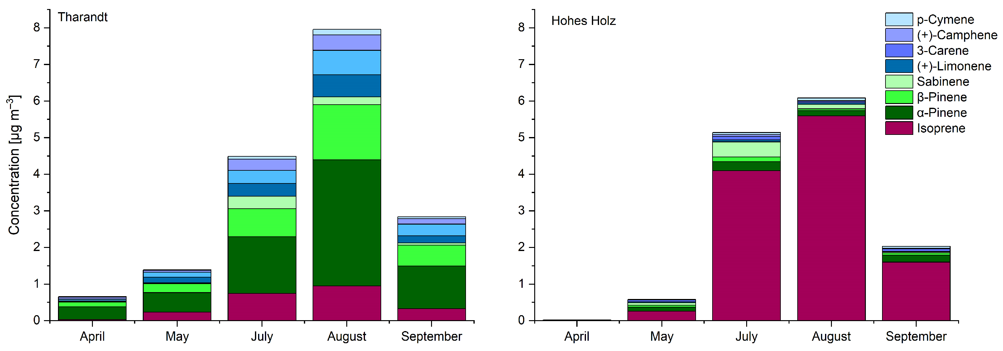
3.2. Seasonal Variation of Terpenes

In addition to isoprene, the monoterpenes α-pinene, β-pinene, sabinene, (+)-camphene, limonene, p-cymene and 3-carene have been unambiguously identified at both sites. Furthermore, an additional peak with low intensity and a mass spectrum with a typical monoterpene pattern is observed in few chromatograms, appearing before the retention time of α-pinene. Based on the comparison of boiling points among potential substances, thujene is hypothesized to be the only monoterpene with a lower boiling point (152 °C) than α-pinene (155 °C). However, the absence of a reference standard for thujene prevents the definitive attribution of this peak.
The measured concentrations (average over the weekly sampling period) of isoprene and monoterpenes for both sampling sites are summarized in Figure 2. The highest concentrations were found in August at both forest sites when the temperatures were also the highest. Average temperatures during sampling at Tharandt were as follows: April 5.9 °C, May: 12.4 °C, July: 19.0 °C, August: 21.5 °C, September: 15.6 °C. The same trend was observed for the sampling site Hohes Holz, where the following temperatures were measured during the sampling periods: April 9.4 °C, May: 12.7 °C, July: 19.5 °C, August: 23.1 °C, September: 16.8 °C.
In contrast to temperature, PAR attains the highest values at both sites in July (Tharandt: 203.6 µmol m−2 s−1 in April, 391.9 µmol m−2 s−1 in May, 516.9 µmol m−2 s−1 in July, 396.9 µmol m−2 s−1 in August and 229.8 µmol m−2 s−1 in September; Hohes Holz: 325.6 µmol m−2 s−1 in April, 379.0 µmol m−2 s−1 in May, 458.8 µmol m−2 s−1 in July, 393.2 µmol m−2 s−1 in August and 230.5 µmol m−2 s−1 in September).
Alpha-pinene was found to be the most dominant compound in the coniferous forest. The concentration increases from April (0.35 µg m−3) to August (3.44 µg m−3) where the maximum is observed. The second major compound is β-pinene. Generally, conifers mainly release monoterpenes with highest concentration of 7 µg m−3 in August. The maximum concentration of isoprene was also observed in August with 0.95 µg m−3, much lower in comparison to monoterpenes.
Isoprene was detected as most abundant compound in the deciduous forest. The average concentration increase from April (0.01 µg m−3) to August (5.59 µg m−3) where the highest concentration was achieved before dropping to 1.6 µg m−3 in September. Monoterpenes (sum of α-pinene, β-pinene, (+)-camphene, sabinene, (+)-limonene, 3-carene and p-cymene) are detected in much lower concentrations. The maximum concentration was observed in July (1.04 µg m−3) and then decreased to 0.49 µg m−3 in August and 0.43 µg m−3 in September. The concentrations in April were near or below the detection limits and increased with the onset of leaf growth and remained high until the end of August. Between June and July, full leaf size is achieved depending on species and weather conditions. Day length and higher temperatures help stimulate the metabolism until August. In September, temperatures begin to drop and cooler temperatures can occur which slows down metabolism and encourages a chemical change within the leaves, resulting in the change in color and, in the end, the fall of leaves.
Considering the distribution of monoterpenes, notable differences can be seen between both forest sites. Consistent with the existing literature data [29], the sampling site Tharandt, characterized by the dominant species European spruce and Scots pine, emits mainly α-pinene and β-pinene. More than 40% of detected monoterpenes can be attributed to α-pinene, while β-pinene vary between 18.9% and 21.1%. The remaining monoterpenes are detectable at lower levels, peaking at a maximum of 15%. The detailed distribution of monoterpenes is shown in Figure 3 including error bars. The distribution of monoterpenes (measured at Tharandt) is comparatively constant over the year and the standard deviation does not exceed 30% for α-pinene and β-pinene. Much higher standard deviations were found for the measurements at Hohes Holz site with European beech and Sessile oak as dominant species. These uncertainties in the measurements result from the very low concentrations of monoterpenes. For example, the highest concentration found in all single measurements at Hohes Holz was only 1.17 µg m−3 in July for sabinene, while α-pinene at the Tharandt site varies between 0.35 µg m−3 (April) and 3.44 µg m−3 with a daily maximum of 7.67 µg m−3 in August. However, it is visible from Figure 3 that sabinene, and partially p-cymene, were detected as dominant monoterpenes in addition to α-pinene. These observations are consistent with those of Holzke et al. [30], where higher emission rates of sabinene from branches of European beech were also found using the branch-enclosure technique. Especially in the summer months, the average concentrations of sabinene are higher (0.41 µg m−3 vs. 0.25 µg m−3) in July or similar (0.13 µg m−3 vs. 0.15 µg m−3) in August in comparison to those of α-pinene. It should be noted, that the standard deviation over all monthly measurements at the Hohes Holz site is more than 70%. The high percentage of p-cymene results from few samples where only p-cymene was detectable at very low concentrations although the monthly average concentration is not really higher in comparison to α-pinene and sabinene.
As can be seen, the assessment of seasonal variability using average values and percentage distributions is subjected to high uncertainties. The reason for this is the temporal variability of concentrations which may change within hours. Furthermore, individual compounds are emitted from trees in different ways. In order to understand between which substances the additional influencing factors lead to different concentrations, we correlated the ambient air concentrations of all individual measurements (each measurement with a temporal resolution of 4 h).
Figure 4 shows the correlation between the concentrations of α-pinene and the other monoterpenes (with the exception of sabinene and p-cymene) observed at Tharandt (coniferous forest). Coefficients of determination above 0.85 indicate a comparable behavior of α-pinene, β-pinene, limonene, 3-carene and camphene, driven by temperature-dependent volatilization. McGlynn et al. [11] separated the contribution from both emission types (light-dependent, and temperature-dependent types) on the basis of diurnal concentration profiles observed in a mixed forest (oak, maple and pine trees). According to these calculations, more than 95% of concentrations of α-pinene and β-pinene can be attributed to temperature-driven emission while a strong light-dependency was found for limonene (~60% and more). These differences, cannot be reproduced with our ambient air measurements from the coniferous forest where α-pinene and limonene show a good correlation. However, a deviating behavior was predicted for sabinene and cymene with a light-dependent component of 100% and 86%, respectively. Also, isoprene belongs to the light-dependent or de novo biosynthesis emitters.
Coefficients of determination of 0.0996 (between α-pinene and isoprene) and 0.1087 (between α-pinene and sabinene) confirm the negligible correlation of the concentration profiles of these substances. If the different emission pathways should be the main driver of temporal concentration profiles, an excellent correlation could be expected between isoprene and sabinene, compounds which are mainly emitted in a light-dependent manner. However, there is no strong correlation between the concentrations of both compounds (R2 = 0.4229). A deviating behavior was also found for p-cymene, which correlates neither with isoprene (R2 = 0.1407) nor with α-pinene (R2 = 0.2213). Therefore, the concentration profiles of isoprene, sabinene, p-cymene and the other monoterpenes are not only influenced by the emission path, but also by other parameters.
Figure 5 shows the correlation between the concentrations of α-pinene and sabinene at the Tharandt site. In contrast to all the other correlations, the concentration profiles show two different groups, one of them with a steep slope and the other one with a shallow slope. The data points in Figure 5 are labeled with the sampling time (middle of the four-hour sampling). While sabinene can be mainly detected during the day (sampling time between 6 am and 10 pm), α-pinene is preferentially detectable in the evening and over the night (sampling time mainly between 8 pm and 8.30 am).
These correlations cannot really be reproduced for the samples from the deciduous forest Hohes Holz. The main reason is, that with exception of isoprene, the concentrations of all the other substances are near or below the detection limit (approximately 0.02 µg m−3 per substance). The uncertainties of measurement increase with decreasing concentrations. Furthermore, the correlation is not possible when one of the substances is not detectable.
Nevertheless, a correlation between the monoterpenes exists (α-pinene vs. β-pinene: R2 = 0.8350; α-pinene vs. 3-carene: R2 = 0.7795; α-pinene vs. limonene: R2 = 0.3515 and α-pinene vs. camphene: R2 = 0.4298). Similar to the other location, no significant correlation can be found between the other substances, not even the grouping between the concentrations of α-pinene and sabinene.

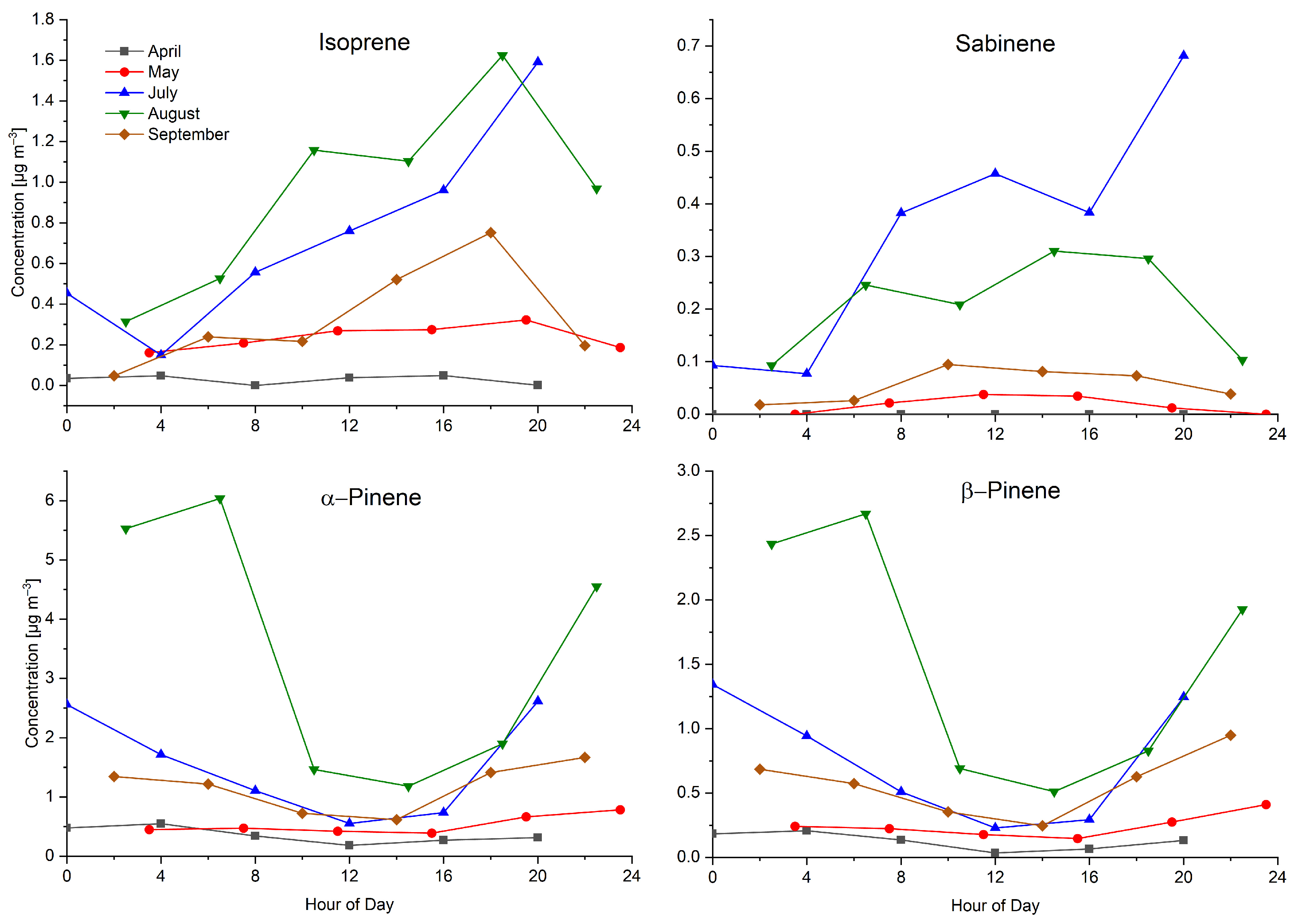
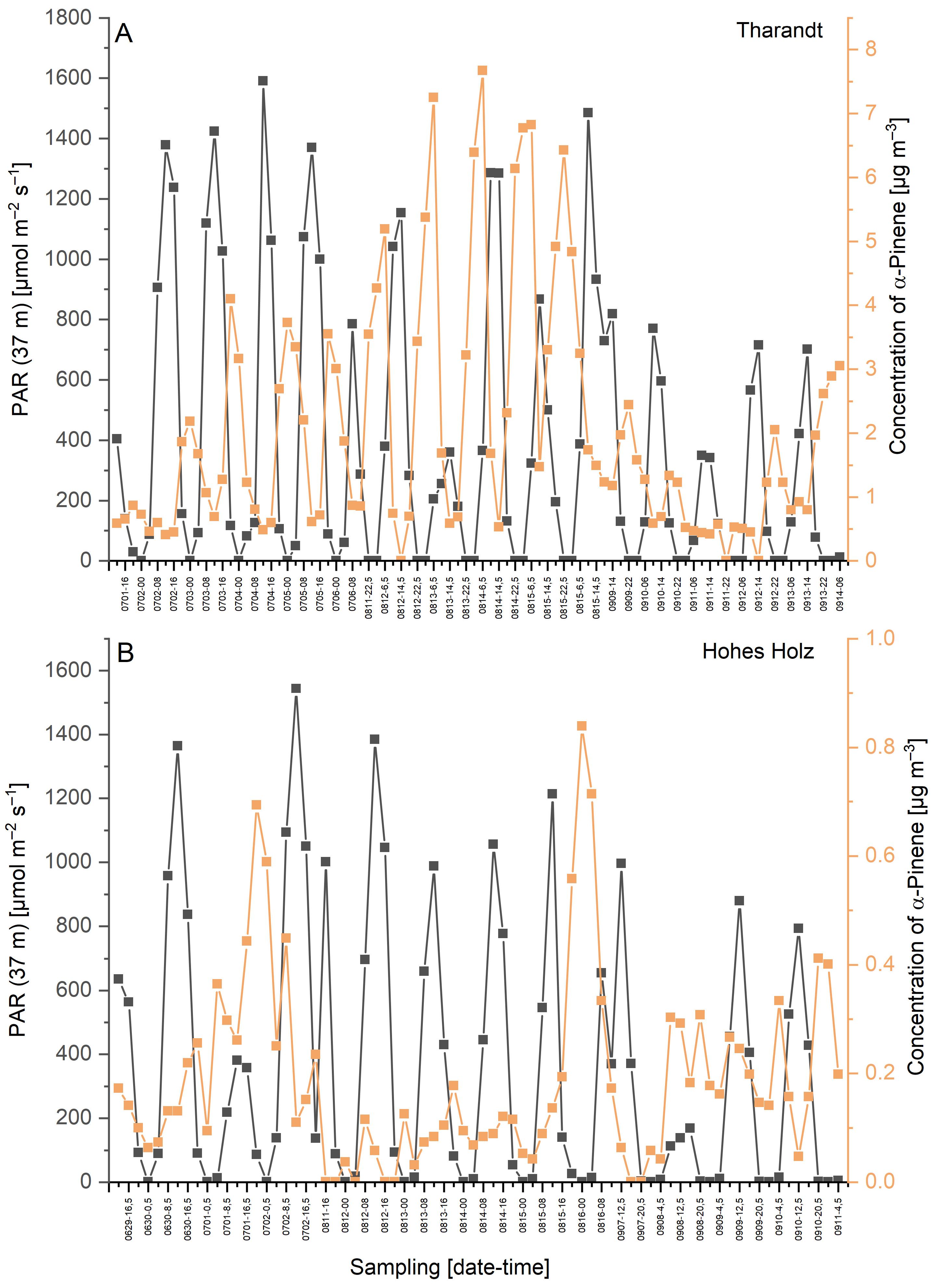
3.3. Diurnal Variation of Terpenes

As described, the concentrations vary over the day. The diurnal variation depends on the emission pathway and the different environmental-influencing parameter. The diurnal trends for our sampling sites are summarized in Figure 6 (coniferous forest in Tharandt) and Figure 7 (deciduous forest Hohes Holz). These figures show the weekly mean concentrations of isoprene, sabinene, α-pinene and β-pinene as examples in dependence on the sampling time over the day. The following conclusions can be drawn from our data: The seasonal concentration trends can be confirmed as described above. Although the concentrations of sabinene and isoprene obtained in the single measurements do not significantly correlate, the diurnal trends are comparable and different from those observed for α-pinene and β-pinene. The latter two compounds also show a comparable diurnal pattern. Generally, the diurnal concentration profiles of compounds are similar for both sampling sites independent of the tree population. These trends are more evident when the concentrations of the substances are higher, in our cases, isoprene and sabinene in deciduous forests and the isomers of pinene in coniferous forests.
Isoprene and sabinene emit in a light-depended manner. Their concentrations show a strong day-time emission. The concentrations increase from the morning and attain their maximum around midday to late afternoon. After that, the concentrations decrease and the nighttime concentrations are near zero. These general trends for isoprene are consistent with those reported in the literature [31]. The deviating behavior of sabinene among the monoterpenes is also in accordance with the observations of McGlynn et al. [11], who found a 100% light-dependent emission pathway for sabinene. Despite the light dependency, the emissions of isoprene and sabinene increase over the day with temperature.
Although the other monoterpenes are emitted in a temperature-dependent manner, different processes influence their detectable concentrations. Midday to afternoon, these compounds are oxidized by photochemically formed radicals due to high solar radiation. Therefore, their concentrations decrease at this time of the day. In contrast to isoprene and sabinene, the concentrations of monoterpenes (with exception of sabinene) are greatest during the night. Comparable diurnal trends for the emissions of monoterpenes from boreal forests were described in the literature [17].

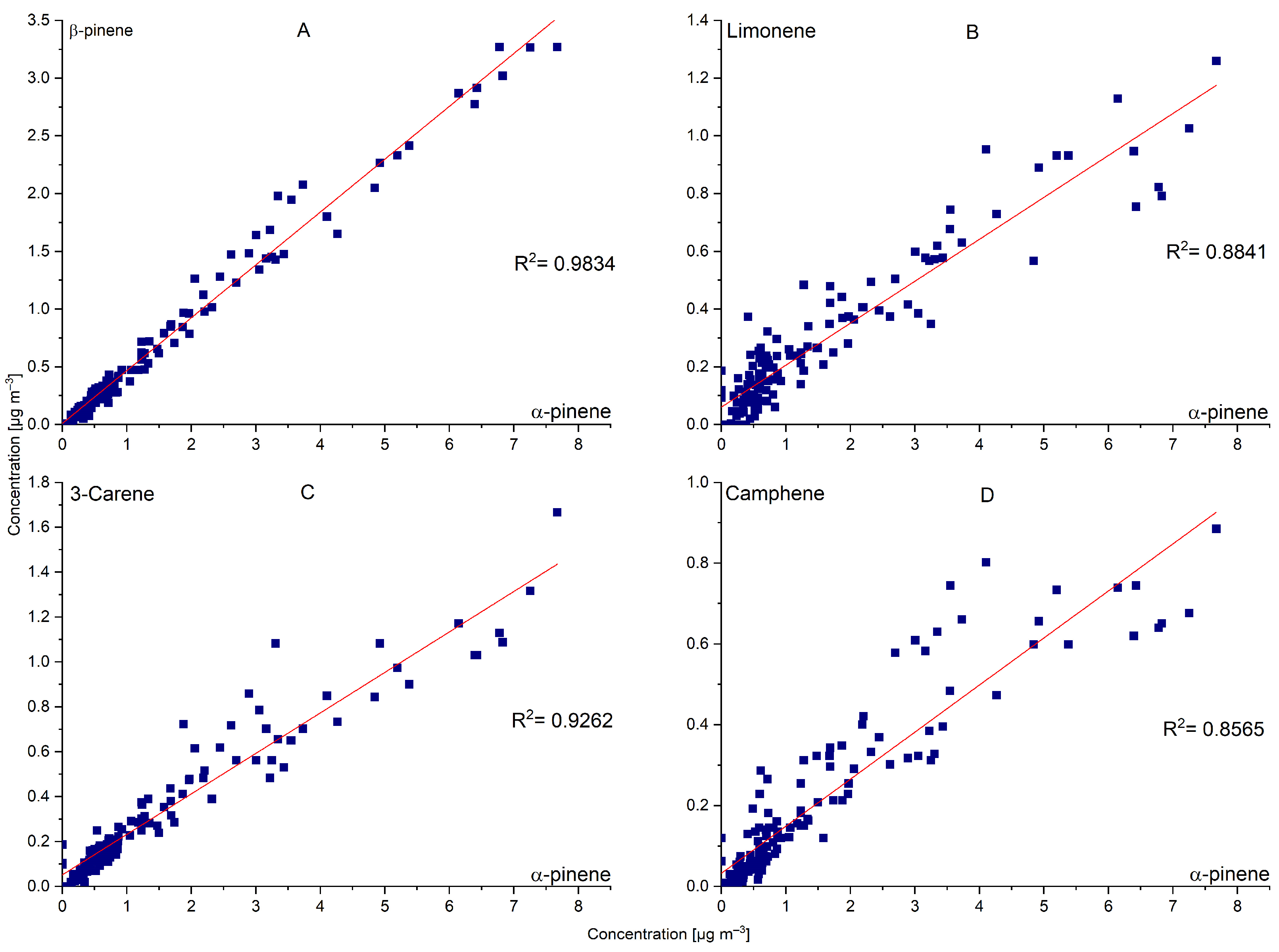
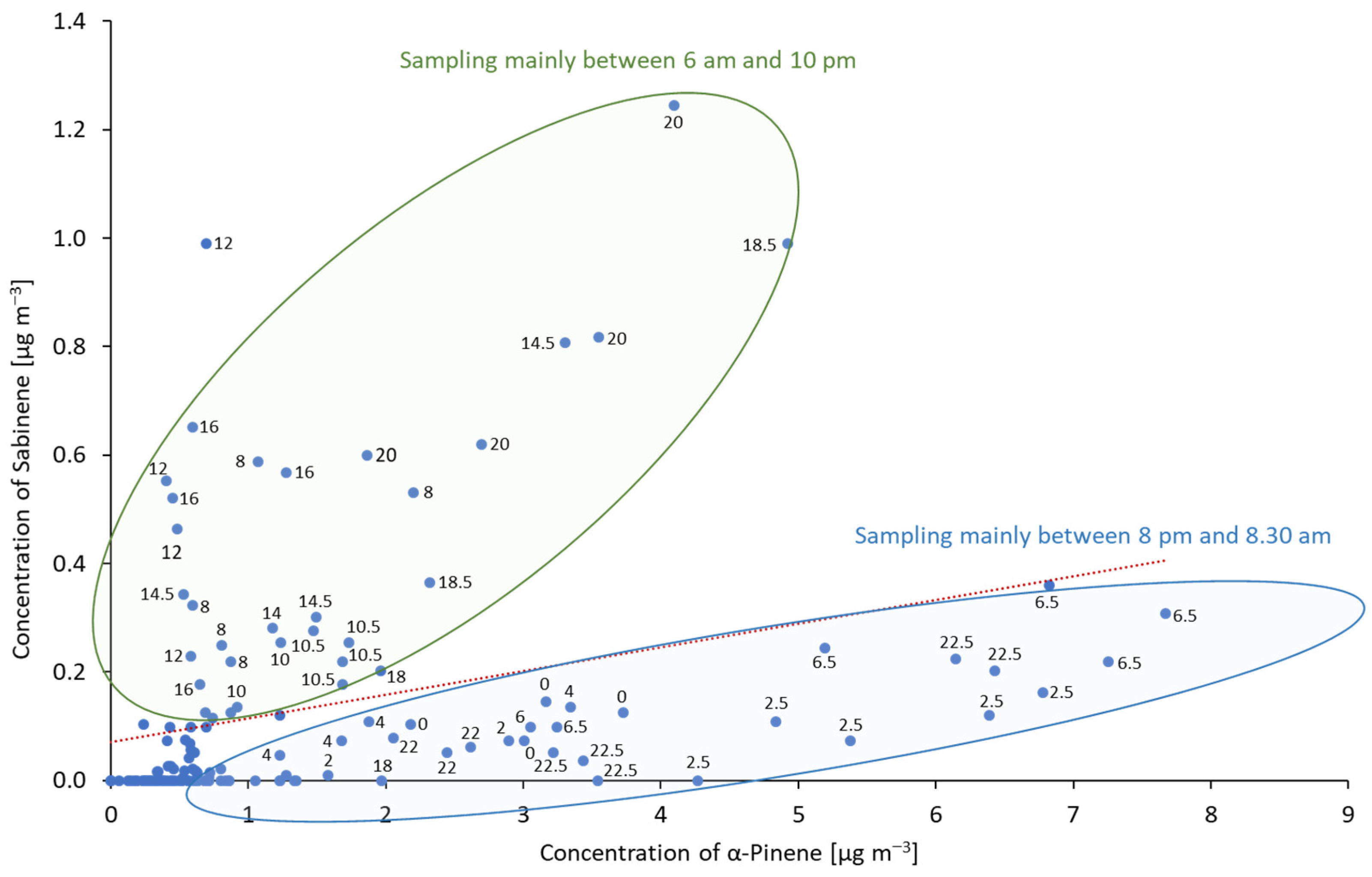
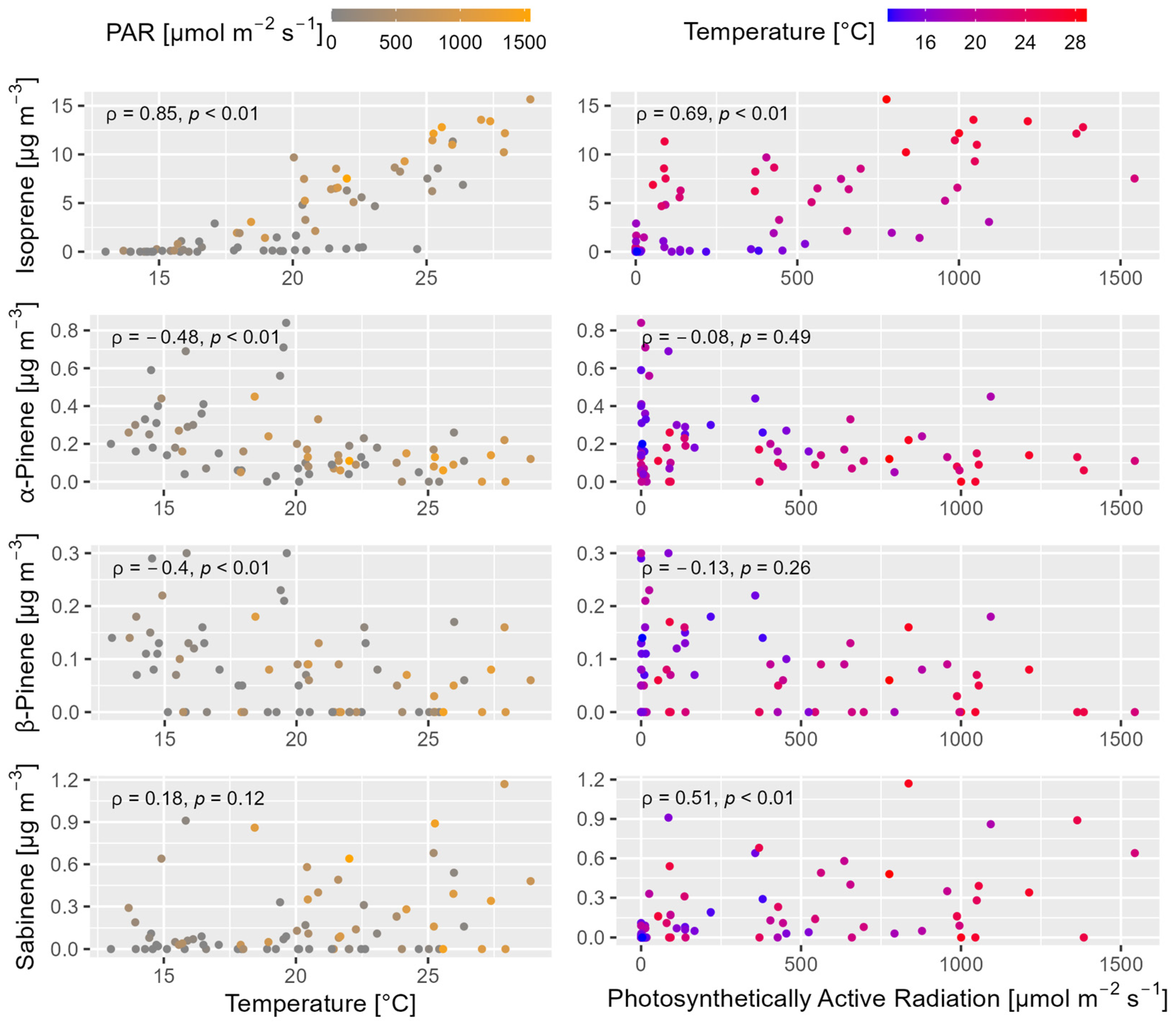
3.4. Correlation of Emissions with Meteorological Parameters

Temperature and photosynthetically active radiation (PAR) were identified as the main drivers of terpene emissions [32]. Both parameters affect the synthesis rates of compounds. Light intensity determines the availability of isoprenoid precursors. Temperature regulates synthase activities and therefore the synthesis of isoprene and monoterpenes due to the temperature-dependent activity of enzymes. Furthermore, temperature affects respiration and influences the formation of isoprenoid intermediates (pyruvate) in the chloroplasts during their biosynthesis [33]. Higher temperatures can also lead to increases in the volatility and diffusion rates of these compounds. As described above, environmental parameters also have an influence on the detectable concentrations in addition to physiological and physicochemical constraints.
Figure 8 shows the temporal variation of the ambient atmospheric concentration of α-pinene and PAR for the months with the highest concentrations of α-pinene (July, August and September) for both sampling sites. As can be clearly seen from Figure 8, high concentrations of α-pinene were found for periods where the PAR was low or zero.
Although PAR was measured at a height of 37 m in Tharandt and the samples were taken in a height of 2 m, an inverse relationship between both parameters is clearly visible. The highest intensities of PAR can be observed midday to early afternoon. As described above, the lowest concentrations of pinene isomers were found in these time periods. Again, these relationships are more clearly visible for the coniferous forest with 10 times higher concentrations of α-pinene.
Further investigations on the correlation of the possible influencing parameters with the concentrations of the separate substances were carried out using Spearman’s rank correlation, which measures the strength and direction of a monotone relationship between two variables without assuming linearity. The Spearman’s rank coefficient ρ can take values between +1 and −1, where ±1 indicates a perfect positive or negative correlation and zero indicates no correlation. The closer ρ is to zero, the weaker is the correlation between the variables. The p-value is a statistical measure of the probability that the observed correlation is due to chance, with small p-values indicating a strong statistical significance. Figure 9 shows the correlation of the concentrations of isoprene, sabinene, α-pinene and β-pinene with temperature and PAR.
The left column in Figure 9 shows the correlations between concentrations and temperature observed at Tharandt. The color of the data points indicates the intensity of PAR (grey: weak, yellow: strong; see caption above the diagrams). Isoprene and sabinene tend to result in the same trend, showing increasing concentrations with increasing temperatures. However, concentrations vary considerably at higher temperatures. In the case of isoprene, the highest concentrations can be observed at low PAR values (grey data points), while concentrations observed at higher values of PAR (yellow) seem to be lower. The variability of concentration at elevated temperatures is much higher for sabinene. Therefore, Spearman’s rank correlation showed a very strong and significant positive correlation between isoprene concentrations and temperature (ρ = 0.85, p < 0.01), while only strong and significant positive correlations were detected between sabinene concentrations and temperature at TW (ρ = 0.69, p < 0.01).
Deviating concentration trends in dependence on temperature were observed for α-pinene and β-pinene. The concentrations increase from about 10 °C to 20 °C and decrease at higher temperatures. Different processes determine this temperature dependence. As shown in Figure 9, higher concentrations were mainly observed when the PAR is low (grey data points). Furthermore, this temperature profile goes along with the activity of flux-controlling enzymes [33]. It must be noted that the temperatures used for these calculations are the air temperatures and not those of the leaf surface. In accordance with the data shown in Figure 8, a negative correlation was observed between PAR and the concentrations of α-pinene and β-pinene. Also, no significant difference was observed between PAR and isoprene or sabinene.
As shown in Figure 10, a very strong significant positive correlation between isoprene concentrations and temperature (ρ = 0.85, p < 0.01) was also observed for the samples from the deciduous forest site Hohes Holz, exactly with the same significance as observed in the coniferous forest. Up to air temperatures of 15 °C, no emission of isoprene was measured. The detectable concentrations increase with rising temperatures. In contrast to the coniferous forest, high concentrations of isoprene are also detectable at high intensities of PAR. The yellow data points indicate that the highest concentrations were found at high temperatures and high light intensities. Therefore, a strong positive correlation was determined between isoprene concentrations and PAR at Hohes Holz (ρ = 0.69, p < 0.01). Similar to coniferous forest, sabinene shows a strong variability in detectable concentrations. Both isomers of pinene show a very weak negative correlation with PAR. Due to the very low concentrations, the temperature-dependent concentration profile as observed in the coniferous forest cannot be seen for the deciduous forest site.
Table 1 summarizes the Spearman’s rank correlation coefficients for the relationship between environmental parameters and the detectable concentrations. Very strong (ρ > 0.8) and strong (ρ > 0.6) correlation degrees with a statistical significance (p < 0.01) [34] are marked. In addition to the above-mentioned correlations, a strong and significant negative correlation between isoprene concentrations and relative humidity (ρ = −0.79, p < 0.01 for Hohes Holz and ρ = −0.77, p < 0.01 for Tharandt) was established for both sampling sites. Furthermore, a strong negative correlation was found between the concentrations of isoprene, α-pinene and sabinene and the soil water content while this correlation is very weak for β-pinene. The O3 concentrations were obtained from nearby public meteorological stations. Only the isoprene concentration in the deciduous forest seems to correlate with the concentration of O3.

4. Summary

The ambient air concentrations of isoprene and monoterpenes in a deciduous and a coniferous forest under comparable meteorological conditions differ considerably. While isoprene is the main compound detectable in the deciduous forest, the isomers of pinene are the most abundant compounds in the ambient atmosphere of the coniferous forest. The concentrations show a strong seasonal and diurnal variability. The identification of themain drivers of variability is quite difficult due to the complexity of influencing parameters. The temporal trends of the individual monoterpenes are quite similar with the exception of sabinene. Our experimental data show that the different emission pathways determine the detectable atmospheric concentrations despite the additional factors influencing the concentration in the air. Sabinene is obviously emitted in a light-dependent manner comparable with isoprene while all the other monoterpenes are emitted by volatilization (in a temperature-dependent way). The detectable concentrations of monoterpenes show a strong negative correlation with light intensity. A high intensity of photosynthetically active radiation leads to reduced concentrations due to the reaction with photochemically formed radicals. Sabinene also shows another behavior here: high concentrations can be also observed at high intensities of light although the atmospheric lifetime of sabinene is comparable with that of α-pinene [12]. The concentrations of the other monoterpenes do not constantly increase with increasing temperatures. The detectable concentrations increase up to an air temperature of approximately 20 °C, after that the concentrations decrease. In addition to the volatilization from storage pools within the trees, the temperature-dependent synthase activities and subsequently the synthesis of most isoprenoids seems to regulate the emissions of monoterpenes [33].

Author Contributions

Conceptualization, H.B. and T.M.; methodology, H.B. and T.M.; validation, H.B. and T.M.; sampling and measurements, H.B., T.M., M.B. and C.R.; discussion of results, H.B., T.M., M.B., M.M. and C.R.; data curation H.B., T.M., M.B. and C.R.; writing—original draft preparation, H.B. and T.M.; writing—review and editing, H.B., T.M., M.B., M.M. and C.R.; supervision, H.B.; project administration, H.B., T.M. and M.B.; funding acquisition, M.M., M.B. and H.B. All authors have read and agreed to the published version of the manuscript.

Funding

The evaluation of data was jointly funded by the Federal Ministry of Food and Agriculture (BMEL) and the Federal Ministry of the Environment, Nature Conservation and Nuclear Safety (BMUV) within the framework of the Forest Climate Fund (grant numbers 2220WK15B4 and 2220WK15A4) managed by the Fachagentur Nachwachsende Rohstoffe e.V. Furthermore, this work was supported by funding from the Helmholtz Association within the framework of MOSES (Modular Observation Solutions for Earth Systems).

Institutional Review Board Statement

Not applicable.

Informed Consent Statement

Not applicable.

Data Availability Statement

The analytical results and data are available from the corresponding author upon request.

Acknowledgments

The authors would like to thank Thomas Grünwald (Dresden University of Technology, Department of Meteorology) for providing the environmental data from the ICOS test site Tharandt.

Conflicts of Interest

The authors declare no conflict of interest.

References

  1. Peñuelas, J.; Staudt, M. BVOCs and global change. Trends Plant Sci. 2010, 15, 133–144. [Google Scholar] [CrossRef] [PubMed]
  2. Schwantes, R.H.; Emmons, L.K.; Orlando, J.J.; Barth, M.C.; Tyndall, G.S.; Hall, S.R.; Ullmann, K.; St. Clair, J.M.; Blake, D.R.; Wisthaler, A.; et al. Comprehensive isoprene and terpene gas-phase chemistry improves simulated surface ozone in the southeastern US. Atmos. Chem. Phys. 2020, 20, 3739–3776. [Google Scholar] [CrossRef]
  3. Salvador, C.M.; Chou, C.C.K.; Ho, T.-T.; Tsai, C.-Y.; Tsao, T.-M.; Tsai, M.-J.; Su, T.-C. Contribution of Terpenes to Ozone Formation and Secondary Organic Aerosols in a Subtropical Forest Impacted by Urban Pollution. Atmosphere 2020, 11, 1232. [Google Scholar] [CrossRef]
  4. Mutzel, A.; Rodigast, M.; Iinuma, Y.; Böge, O.; Herrmann, H. Monoterpene SOA—Contribution of first-generation oxidation products to formation and chemical composition. Atmos. Environ. 2016, 130, 136–144. [Google Scholar] [CrossRef]
  5. Mu, Z.; Llusia, J.; Zeng, J.; Zhang, Y.; Asensio, D.; Yang, K.; Yi, Z.; Wang, X.; Penuelas, J. An Overview of the Isoprenoid Emissions from Tropical Plant Species. Front. Plant Sci. 2022, 13, 833030. [Google Scholar] [CrossRef]
  6. Lun, X.; Lin, Y.; Chai, F.; Fan, C.; Li, H.; Liu, J. Reviews of emission of biogenic volatile organic compounds (BVOCs) in Asia. J. Environ. Sci. 2020, 95, 266–277. [Google Scholar] [CrossRef]
  7. Ferracci, V.; Bolas, C.G.; Freshwater, R.A.; Staniaszek, Z.; King, T.; Jaars, K.; Otu-Larbi, F.; Beale, J.; Malhi, Y.; Waine, T.W.; et al. Continuous Isoprene Measurements in a UK Temperate Forest for a Whole Growing Season: Effects of Drought Stress during the 2018 Heatwave. Geophys. Res. Lett. 2020, 47, e2020GL088885. [Google Scholar] [CrossRef]
  8. Antonelli, M.; Donelli, D.; Barbieri, G.; Valussi, M.; Maggini, V.; Firenzuoli, F. Forest Volatile Organic Compounds and Their Effects on Human Health: A State-of-the-Art Review. Int. J. Environ. Res. Public Health. 2020, 17, 6506. [Google Scholar] [CrossRef]
  9. Kopaczyk, J.M.; Warguła, J.; Jelonek, T. The variability of terpenes in conifers under developmental and environmental stimuli. Environ. Exp. Bot. 2020, 180, 104197. [Google Scholar] [CrossRef]
  10. Lerdau, M.; Guenther, A.; Monson, R. Plant Production and Emission of Volatile Organic Compounds. BioScience 1997, 47, 373–383. [Google Scholar] [CrossRef]
  11. McGlynn, D.F.; Frazier, G.; Barry, L.E.R.; Lerdau, M.T.; Pusede, S.E.; Isaacman-VanWertz, G. Minor contributions of daytime monoterpenes are major contributors to atmospheric reactivity. Biogeosciences 2023, 20, 45–55. [Google Scholar] [CrossRef]
  12. Atkinson, R.; Arey, J. Gas-phase tropospheric chemistry of biogenic volatile organic compounds: A review. Atmos. Environ. 2003, 37, 197–219. [Google Scholar] [CrossRef]
  13. Guenther, A. Biological and Chemical Diversity of Biogenic Volatile Organic Emissions into the Atmosphere. ISRN Atmos. Sci. 2013, 2013, 786290. [Google Scholar] [CrossRef]
  14. Meneguzzo, F.; Albanese, L.; Bartolini, G.; Zabini, F. Temporal and Spatial Variability of Volatile Organic Compounds in the Forest Atmosphere. Int. J. Environ. Res. Public Health 2019, 16, 4915. [Google Scholar] [CrossRef]
  15. McGlynn, D.F.; Barry, L.E.R.; Lerdau, M.T.; Pusede, S.E.; Isaacman-VanWertz, G. Measurement report: Variability in the composition of biogenic volatile organic compounds in a Southeastern US forest and their role in atmospheric reactivity. Atmos. Chem. Phys. 2021, 21, 15755–15770. [Google Scholar] [CrossRef]
  16. Hakola, H.; Taipale, D.; Praplan, A.; Schallhart, S.; Thomas, S.; Tykkä, T.; Helin, A.; Bäck, J.; Hellén, H. High variations of BVOC emissions from Norway spruce in boreal forests. Atmos. Chem. Phys. Discuss. 2022, 2022, 1–29. [Google Scholar] [CrossRef]
  17. Hakola, H.; Hellén, H.; Hemmilä, M.; Rinne, J.; Kulmala, M. In situ measurements of volatile organic compounds in a boreal forest. Atmos. Chem. Phys. 2012, 12, 11665–11678. [Google Scholar] [CrossRef]
  18. Yu, H.; Guenther, A.; Gu, D.; Warneke, C.; Geron, C.; Goldstein, A.; Graus, M.; Karl, T.; Kaser, L.; Misztal, P.; et al. Airborne measurements of isoprene and monoterpene emissions from southeastern U.S. forests. Sci. Total Environ. 2017, 595, 149–158. [Google Scholar] [CrossRef]
  19. Lee, J.H.; Batterman, S.A.; Jia, C.; Chernyak, S. Ozone artifacts and carbonyl measurements using Tenax GR, Tenax TA, Carbopack B, and Carbopack X adsorbents. J. Air Waste Manag. Assoc. 2006, 56, 1503–1517. [Google Scholar] [CrossRef]
  20. Helmig, D. Ozone removal techniques in the sampling of atmospheric volatile organic trace gases. Atmos. Environ. 1997, 31, 3635–3651. [Google Scholar] [CrossRef]
  21. Fick, J.; Pommer, L.; Andersson, B.; Nilsson, C. Ozone Removal in the Sampling of Parts per Billion Levels of Terpenoid Compounds:  An Evaluation of Different Scrubber Materials. Environ. Sci. Technol. 2001, 35, 1458–1462. [Google Scholar] [CrossRef]
  22. Pollmann, J.; Ortega, J.; Helmig, D. Analysis of Atmospheric Sesquiterpenes:  Sampling Losses and Mitigation of Ozone Interferences. Environ. Sci. Technol. 2005, 39, 9620–9629. [Google Scholar] [CrossRef]
  23. Mermet, K.; Sauvage, S.; Dusanter, S.; Salameh, T.; Léonardis, T.; Flaud, P.-M.; Perraudin, É.; Villenave, É.; Locoge, N. Optimization of a gas chromatographic unit for measuring biogenic volatile organic compounds in ambient air. Atmos. Meas. Tech. 2019, 12, 6153–6171. [Google Scholar] [CrossRef]
  24. Kootstra, P.R.; Herbold, H.A. Automated solid-phase extraction and coupled-column reversed-phase liquid chromatography for the trace-level determination of low-molecular-mass carbonyl compounds in air. J. Chromatogr. A 1995, 697, 203–211. [Google Scholar] [CrossRef]
  25. Greenberg, J.P.; Lee, B.; Helmig, D.; Zimmerman, P.R. Fully automated gas chromatograph-flame ionization detector system for the in situ determination of atmospheric nonmethane hydrocarbons at low parts per trillion concentration. J. Chromatogr. A 1994, 676, 389–398. [Google Scholar] [CrossRef]
  26. Helmig, D.; Greenberg, J. Artifact formation from the use of potassium-iodide-based ozone traps during atmospheric sampling of trace organic gases. J. High Resolut. Chrom. 1995, 18, 15–18. [Google Scholar] [CrossRef]
  27. Helin, A.; Hakola, H.; Hellén, H. Optimisation of a thermal desorption–gas chromatography–mass spectrometry method for the analysis of monoterpenes, sesquiterpenes and diterpenes. Atmos. Meas. Tech. 2020, 13, 3543–3560. [Google Scholar] [CrossRef]
  28. Mayer, T.; Cämmerer, M.; Borsdorf, H. A versatile and compact reference gas generator for calibration of ion mobility spectrometers. Int. J. Ion Mobil. Spectrom. 2020, 23, 51–60. [Google Scholar] [CrossRef]
  29. Malik, T.G.; Gajbhiye, T.; Pandey, S.K. Plant specific emission pattern of biogenic volatile organic compounds (BVOCs) from common plant species of Central India. Environ. Monit. Assess. 2018, 190, 631. [Google Scholar] [CrossRef]
  30. Holzke, C.; Dindorf, T.; Kesselmeier, J.; Kuhn, U.; Koppmann, R. Terpene emissions from European beech (shape Fagus sylvatica L.): Pattern and Emission Behaviour Over two Vegetation Periods. J. Atmos. Chem. 2006, 55, 81–102. [Google Scholar] [CrossRef]
  31. Ghirardo, A.; Koch, K.; Taipale, R.; Zimmer, I.; Schnitzler, J.P.; Rinne, J. Determination of de novo and pool emissions of terpenes from four common boreal/alpine trees by 13CO2 labelling and PTR-MS analysis. Plant Cell Environ. 2010, 33, 781–792. [Google Scholar] [CrossRef] [PubMed]
  32. Vettikkat, L.; Miettinen, P.; Buchholz, A.; Rantala, P.; Yu, H.; Schallhart, S.; Petäjä, T.; Seco, R.; Männistö, E.; Kulmala, M.; et al. High emission rates and strong temperature response make boreal wetlands a large source of isoprene and terpenes. Atmos. Chem. Phys. 2023, 23, 2683–2698. [Google Scholar] [CrossRef]
  33. Niinemets, Ü.; Loreto, F.; Reichstein, M. Physiological and physicochemical controls on foliar volatile organic compound emissions. Trends Plant Sci. 2004, 9, 180–186. [Google Scholar] [CrossRef] [PubMed]
  34. Yan, Z.; Wang, S.; Ma, D.; Liu, B.; Lin, H.; Li, S. Meteorological Factors Affecting Pan Evaporation in the Haihe River Basin, China. Water 2019, 11, 317. [Google Scholar] [CrossRef]
Figure 1. Signal intensities of α-pinene, 3-carene and limonene after preconcentration of 19.2 L air with defined concentrations produced in a reference gas generator with and without O3 scrubber under different conditions (A) and signal intensities of O3 artifacts observed with and without scrubber (B).
Atmosphere 14 01347 g001
Figure 2. Average concentration (µg m−3) of isoprene and monoterpenes over the one-week measurement campaigns at Tharandt (coniferous forest) and Hohes Holz (deciduous forest) in 2022.
Atmosphere 14 01347 g002
Figure 3. Average percentage distribution of monoterpenes during the one-week sampling periods.
Atmosphere 14 01347 g003
Figure 4. Correlation of the concentrations (µg m−3) of monoterpenes (α-pinene vs. (A) β-pinene, (B) Limonene, (C) 3-Carene and (D) Camphene) observed during monthly measurements 2022 at Tharandt (coniferous forest).
Atmosphere 14 01347 g004
Figure 5. Correlation of the concentrations (µg m−3) of sabinene vs. α-pinene at Tharandt (coniferous forest). The points in the diagram are labeled with sampling time (±2 h).
Atmosphere 14 01347 g005
Figure 6. Seasonal and diurnal profile of measured concentrations of isoprene and monoterpenes in dependence on sampling time. The average concentrations for the respective sampling time are shown for the weekly samplings (Tharandt: coniferous forest).
Atmosphere 14 01347 g006
Figure 7. Seasonal and diurnal profile of measured concentrations of isoprene and monoterpenes in dependence on sampling time. The average concentrations for the respective sampling time are shown for the weekly samplings (Hohes Holz: deciduous forest).
Atmosphere 14 01347 g007
Figure 8. Profile of photosynthetically active radiation (PAR, 400 to 700 nm) taken at a height of 37 m and the concentration of α-pinene in the coniferous (A) and deciduous (B) forests. The figure shows the acyclic behavior only for the sampling periods in July, August and September because the measurable concentrations were high enough.
Atmosphere 14 01347 g008
Figure 9. Correlation between concentrations of selected compounds and temperature or photosynthetically active radiation at the Tharandt site.
Atmosphere 14 01347 g009
Figure 10. Correlation between concentrations of selected compounds and temperature or photosynthetically active radiation at the Hohes Holz site.
Atmosphere 14 01347 g010
Table 1. Spearman’s rank correlation coefficients for the relationship between the concentrations of isoprene, sabinene, isomers of pinene and different environmental parameters.
ParameterIsopreneα-Pineneβ-PineneSabinene
Concentration (µg m−3)
Tharandt
PAR (µmol m−2 s−1) 1ρ = 0.34, p < 0.01ρ = −0.28 p < 0.01ρ = −0.35, p < 0.01ρ = 0.31, p < 0.01
Temperature (°C)ρ = 0.85, p < 0.01ρ = 0.57, p < 0.01ρ = 0.50, p < 0.01ρ = 0.69, p < 0.01
Relative humidity (%)ρ = −0.77, p < 0.01ρ = −0.33, p < 0.01ρ = −0.24, p < 0.01ρ = −0.41, p < 0.01
Ozone (µg L−1)ρ = 0.46, p < 0.01ρ = −0.09, p = 0.271ρ = −0.16, p = 0.05ρ = 0.126, p = 0.14
Windspeed (m s−1)ρ = −0.19, p = 0.03ρ = −0.26, p < 0.01ρ = −0.24, p < 0.01ρ = −0.27, p < 0.01
Soil temperature (°C) 1ρ = 0.33, p < 0.01ρ = 0.50, p < 0.01ρ = 0.50, p < 0.01ρ = 0.35, p < 0.01
SWC (%) 1ρ = −0.67, p < 0.01ρ = −0.63, p < 0.01ρ = −0.06, p < 0.01ρ = −0.63, p < 0.01
Hohes Holz
PAR (µmol m−2 s−1) 1ρ = 0.69, p < 0.01ρ = −0.08, p = 0.49ρ = −0.13, p = 0.26ρ = 0.51, p < 0.01
Temperature (°C)ρ = 0.85, p < 0.01ρ = −0.48, p < 0.01ρ = −0.40, p < 0.01ρ = 0.18, p = 0.12
Relative humidity (%)ρ = −0.79, p < 0.01ρ = 0.55, p < 0.01ρ = 0.50, p < 0.01ρ = −0.09, p = 0.46
Ozone (µg L−1)ρ = 0.70, p < 0.01ρ = −0.09, p < 0.01ρ = −0.22, p = 0.07ρ = 0,15, p = 0.19
Windspeed (m s−1)ρ = 0.00, p = 0.97ρ = −0.21, p = 0.08ρ = −0.06, p = 0.61ρ = −0.07, p = 0.55
Soil temperature (°C) 1ρ = 0.01, p = 0.92ρ = −0.11, p = 0.34ρ = −0.25, p = 0.03ρ = −0.19, p = 0.11
SWC (%) 1ρ = −0.13, p = 0.25ρ = 0.40, p < 0.01ρ = 0.43, p < 0.01ρ = 0.32, p < 0.01
1 The photosynthetically active radiation (PAR) was taken at a height of 37 m, the soil temperature and the soil water content (SWC) were measured at a depth of 0.5 m (bold: significant correlations, green: strong and very strong positive significant correlations, red: strong and very strong negative significant correlations).
Disclaimer/Publisher’s Note: The statements, opinions and data contained in all publications are solely those of the individual author(s) and contributor(s) and not of MDPI and/or the editor(s). MDPI and/or the editor(s) disclaim responsibility for any injury to people or property resulting from any ideas, methods, instructions or products referred to in the content.

